Spatiotemporal Modeling of Urban Growth Using Machine Learning


Research in Spatial Economics (RiSE) Group, Department of Mathematical Sciences, EAFIT University, Carrera 48 A 10 Sur 107, Casa 4, 050022 Medellín, Antioquia, Colombia
*
Author to whom correspondence should be addressed.
†
These authors contributed equally to this work.
Remote Sens. 2020, 12(1), 109; https://doi.org/10.3390/rs12010109
Submission received: 1 December 2019
/
Revised: 20 December 2019
/
Accepted: 21 December 2019
/
Published: 28 December 2019
(This article belongs to the Special Issue Machine Learning of Remote Sensing Data for Urban Growth Analysis and Modeling)
Abstract
:This paper presents a general framework for modeling the growth of three important variables for cities: population distribution, binary urban footprint, and urban footprint in color. The framework models the population distribution as a spatiotemporal regression problem using machine learning, and it obtains the binary urban footprint from the population distribution through a binary classifier plus a temporal correction for existing urban regions. The framework estimates the urban footprint in color from its previous value, as well as from past and current values of the binary urban footprint using a semantic inpainting algorithm. By combining this framework with free data from the Landsat archive and the Global Human Settlement Layer framework, interested users can get approximate growth predictions of any city in the world. These predictions can be improved with the inclusion in the framework of additional spatially distributed input variables over time subject to availability. Unlike widely used growth models based on cellular automata, there are two main advantages of using the proposed machine learning-based framework. Firstly, it does not require to define rules a priori because the model learns the dynamics of growth directly from the historical data. Secondly, it is very easy to train new machine learning models using different explanatory input variables to assess their impact. As a proof of concept, we tested the framework in Valledupar and Rionegro, two Latin American cities located in Colombia with different geomorphological characteristics, and found that the model predictions were in close agreement with the ground-truth based on performance metrics, such as the root-mean-square error, zero-mean normalized cross-correlation, Pearson’s correlation coefficient for continuous variables, and a few others for discrete variables such as the intersection over union, accuracy, and the metric. In summary, our framework for modeling urban growth is flexible, allows sensitivity analyses, and can help policymakers worldwide to assess different what-if scenarios during the planning cycle of sustainable and resilient cities.
1. Introduction
The rapid urbanization of cities is a global trend that poses challenges and opportunities for our long-term sustainability. As the population grows [1] and people continue to migrate to urban centers [2,3], problems related to poverty traps [4], informal settlements, insecurity, air pollution, noise, visual contamination, fast-spreading diseases [5], and the economic cost of expanding public infrastructure become more relevant. Cities consume raw materials in large quantities [6], which accelerates the degradation of the environment [7,8] and worsens climate change [9,10,11,12]. However, cities are also beacons of hope as they provide opportunities to their inhabitants to access to basic utilities (e.g., water, electricity, gas, internet), health facilities, employment with competitive wages, financial services, entertainment, technical training, formal education, and much more [13,14]. When diverse and skilled human capital interacts, cities can boost ecosystems of research, development, innovation, and entrepreneurship [15,16,17]. It is this duality between the challenges and benefits of cities that makes the understanding of their growth so important for us.
To predict how cities are going to look like in the future, urban planners rely on historical data and urban growth models [10,18,19,20]. These models can have multiple outputs, but they commonly provide estimations of binary urban footprints (i.e., maps with urban or non-urban categories) or population distribution within a region of study over time [21]. The urban growth models help local governments to estimate required investments in public infrastructures, such as roads, hospitals, schools, housing projects, and amenities, as well as in sustainable urban development [22,23,24]. Utility companies use urban growth predictions to forecast demand in public services and to plan investments and interventions in their networks. As cities grow, they consume their surrounding land, and for this reason, policymakers and planners need urban growth predictions for preventing communities from building in protected areas (e.g., wetlands, national parks, reserved lands for indigenous communities, etc.) or terrains prone to natural hazards, such as floods, landslides, and volcanic eruptions, among others [25,26,27]. Urban growth is also important for Economists as they use growth forecasts as input features in different econometric analyses [28,29,30].
With the premise that the population drives the urbanization, it is possible to use population growth models to estimate binary urban growth using a classifier, by assigning urban or non-urban labels to each piece of land. This classifier can be as simple as stating that a piece of land gets urbanized when the number of inhabitants increases above a certain threshold or it can consider a spatiotemporal neighborhood in the decision. In general, population growth modeling is an active research area in fields as diverse as Ecology, Economics [31], and Geography [32,33,34], and the related studies use model-driven [23,35,36] or data-driven approaches [37,38,39]. In model-driven studies, researchers define the model beforehand [31], either based on physics [40] or intuition of the problem at hand and then determine its coefficients through an optimization process over the available data, a process known as parameter identification. In the data-driven approach, researchers pose fewer constraints as to the specific model to use but they can propose different model families to find the one that best fits the observed data. While model-driven approaches provide superior interpretability, they cannot capture unexpected patterns. In contrast, data-driven models are often not as interpretable, but they capture complex dynamics, improving the match between the predictions and the observed phenomena. Breakthroughs in the generalization capability of data-driven models are commonly correlated with the availability of large and representative input datasets.
The early literature on population growth was more inclined towards model-driven than data-driven approaches [35,41]. Early population growth models focused on the temporal component, using the historical records of population as time series that could be modeled through simple regression models, very often, logistic functions. The rationale behind the use and widespread of the logistic function for population growth modeling is threefold. Firstly, it represents the slow initial growth that follows the settlement of a population on a piece of land; secondly, it captures the fast and steady growth of that population when it thrives in a suitable environment; and thirdly, it shows the slow asymptotic growth of the same population when it approaches the maximum capacity of the environment and has to adapt itself to limited resources. This logistic growth is mathematically modeled through a differential equation where the time is the independent variable. However, over time, authors included the spatial effects [42], initially through decoupled spatiotemporal differential equations and then through coupled spatiotemporal stochastic differential equations. However, as the analytical models became more and more complex, exact solutions became harder to find, and numerical methods became a reasonable alternative, and with them, the data-driven approach gained visibility in the literature. Researchers have explored data-driven approaches based on cellular automata [38] and machine learning models, such as Hidden Markov Models (HMM), spatiotemporal Gaussian Process (GP) regressions, and recurrent neural networks (RNN), to name a few.
Arguably, the most used urban growth model today is SLEUTH, a cellular automaton (i.e., a rule-based algorithm) introduced about two decades ago [43,44]. The SLEUTH model is simple to understand because it captures logical urban growth patterns from a few selected input variables. However, it has a few limitations: (i) it is not straightforward to extend the model if you want to include new variables (e.g., amenities, natural risks, violence, land price, socio-economic distribution, availability of public services, etc.) and assess their impact. The main reason is that every new variable that you include in the model requires a new hand-crafted rule; (ii) the SLEUTH model only considers fixed spatial neighborhoods for the variables, but the spatial influence of all variables in the model is not necessarily the same, and (iii) the SLEUTH model is not driven by population growth as it happens in most cities (knowing that there are exceptions, like some new cities in China that get built in advance of the population arrival).
The main contribution of this paper is the proposal of an urban-growth framework that is simple but with good explanatory power (i.e., a parsimonious model), driven by population, and based on machine learning. The user can train the underlying models with few open worldwide-available data, namely, population distribution maps from the Global Human Settlement Layer (GHSL: [45]) and the satellite imagery from the NASA/USGS Landsat program, although in the future it could include data from the European Copernicus program as it provides better spatial and temporal resolutions simplifying the acquisition of cloud-free images, particularly in the tropic. This is because the European Copernicus program provides satellite images with pixel sizes of 20 × 20 for some bands and 10 × 10 for others, with a revisit time of about 5 day. In comparison, the Landsat program provides satellite images with a pixel size of 30 × 30 and a revisit time of 16 day.
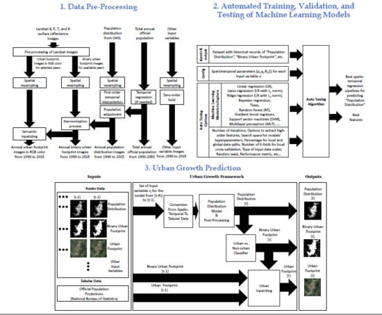
The proposed urban-growth framework is flexible enough to easily handle additional input variables as long their historical records exist over a common period; if this is not the case, they can be included under the assumption that they do not change much over time using a zero-order hold. The framework is entirely data-driven and capable of learning different growth patterns across different geographies. All of these characteristics make the framework suitable for data-constrained scenarios, as well as for large-scale comparative studies, and specialized consultancies in urban expansion, service provisioning, environmental monitoring, among others. The urban-growth framework can be applied worldwide by cities with budget constraints that cannot afford to purchase high-quality commercial data as the core data that the model needs are open satellite imagery, a characteristic that can enable low-budget studies. Figure 1 presents a simplified diagram of the urban growth framework that we develop in this paper.
This paper is organized as follows. Section 2 describes the materials and methods. It explains the input variables, pre-processing stages, adopted terminology, and mathematical formulation of the proposed urban growth framework, as well as the post-processing stages. Section 2 also describes the strategies for training, selecting the optimal parameters for the growth model and testing it with historical data. Section 2 concludes with the implementation details of the urban growth framework and a brief description of Rionegro and Valledupar, the two selected cities in Latin America for the case studies. Section 3 presents basic demographic and urban diagnostic graphs of these two cities, as well as the results of training, validating, and testing the urban growth framework. Section 3 concludes with the spatiotemporal urban predictions for Rionegro and Valledupar from 2020 to 2050. Finally, Section 4 discusses the obtained results, while Section 5 presents the conclusions of this paper and future work.
2. Materials and Methods
In this work, we consider that a pixel is urban if it is detected as built-up land in the Landsat images and its associated population is above a defined threshold, following the same rationale as the urban-center definition of the GHS Urban Centre Database 2015 [46]. We discuss the process to find the optimal threshold for the identification of urban areas in the historical Landsat-image series in Section 2.2.4. With the definition of what makes a pixel urban, we can apply it to a single city or a larger conurbation area in the same way, as it is independent of administrative boundaries.
2.1. Input Variables
The input variables for the urban growth model are described in Table 1. The table includes the name, source, digital format (i.e., raster or vector), original resolution (i.e., pixel size for raster data), availability (i.e., local, national, or global), and the variable’s importance for the growth model (i.e., essential or optional). The population distribution, the binary urban footprint, and the urban footprint in color are essential variables in our framework, but additional variables can be included subject to availability for assessing their impact or for improving the spatiotemporal urban estimates.
2.2. Data Pre-Processing
The pre-processing of the input variables is illustrated in Figure 2, and the key blocks are described in the next subsections. The overall pre-processing includes:
- Using images from Landsat missions to obtain a set of initial estimates of the urban footprint in RGB color and the binary urban footprint. This is covered in Section 2.2.1.
- Performing a content-aware spatial resampling of all input variables for getting digital images with a common coordinate reference system, geographic extent, and spatial resolution. This is explained in Section 2.2.2.
- Applying a first-order temporal interpolation to the population distribution for getting annual estimates, and optionally if available, applying an adjustment of the annual population distribution estimates to match the total population defined by the corresponding National Bureau of Statistics (see Section 2.2.3). Notice that, if the official population values are only available for a subset of the years of interest, then a temporal regression is applied to estimate the values in missing years.
- Estimating the binary urban footprint for missing years by harmonizing it with the historical population distribution. This process is detailed in Section 2.2.4;
- Using a semantic-inpainting algorithm for estimating the urban footprint in RGB color for missing years. The block in this pre-processing stage is the same to the one explained in Section 2.6.
- Applying a zero-order hold to get annual estimates of the other input variables in missing years.
At the end of the pre-processing, the intermediate input dataset has annual estimates of the different spatial variables at least between 1990 and 2015, using a common coordinate reference system, geographic extent, and spatial resolution. Additionally, there are no pixel values in the dataset with NoData, NaN, , or . Finally, in case of using the official population information, this should cover at least the period from 1990 to the final simulation year, which was set to 2050 for our two case studies.
2.2.1. Pre-Processing of Landsat Images
We used the images from Landsat missions 4, 5, 7, and 8 with atmospheric correction as a starting point for the data pre-processing that is expanded in Figure 3. We started by creating a mask for the clouds and their shadows using the quality assessment band that comes with the Landsat images, and then grew it by applying two consecutive dilation-based morphological filters with a box-shaped structuring element of pixels at the original spatial resolution (i.e., a pixel size of about 30 × 30 ). Then, we applied a relative radiometric normalization using the pseudo-invariant features method described in [56,57] using the RStoolbox library in R. Afterwards, we filled the missing “NoData” values left by the removal process of clouds and shadows by using a simple inpainting process. We took the average of adjacent images when these were available; otherwise, we filled the “NoData” by copying the values from the nearest image in time. As a last step, we removed the quality-assessment band from the intermediate results and kept processing only the images with seven bands and without clouds or shadows.
With the pre-processed Landsat images, we extracted the RGB true-color composite. For the Landsat missions 4 TM, 5 TM, and 7 ETM+, we combined the bands , , and , whereas for Landsat mission 8 OLI, we combined the bands , , and . We then selected the best images based on the perceived visual quality obtaining a set of urban footprint images in RGB color for selected years. We also used the pre-processed Landsat images to extract the binary urban footprint. Firstly, we assembled a multi-temporal dataset of pixels with four categories: “built-up”, “vegetation”, “bare soil”, and “water”, respectively. In this process, we randomly selected groups of pixels across different years and labeled them using on-screen interpretation and reference data (for one year) from the master plan’s land-use map. At this point, the collected data for each sampled pixel included the seven bands from the pre-processed Landsat images, as well as its corresponding category. Once the dataset was assembled, we split it into three non-overlapping datasets for training (49%), validation (21%), and testing (30%). We used the training and validation datasets to train a random forest classifier and find the best hyper-parameters using the built-in random grid-search methods in the Caret library in R. After the training, we extracted the performance metrics of the classifier on the testing dataset and proceeded to classify the entire set of the pre-processed Landsat images. Then, we performed a reclassification of the results using only two categories, one for “urban” pixels (built-up) and the other one for “non-urban” pixels (i.e., either “vegetation”, or “bare soil”, or “water”). Reclassifying the four categories into two was more accurate than training a binary classifier directly from the available data. After the reclassification, we filled the small patches that may remain using a morphological operation known as closing, which corresponds to a dilation followed by an erosion.
The final step of the pre-processing included a two-step temporal correction, depicted in Figure 4, that was adapted from the inter-annual series correction proposed by Cao et al. [58]. The temporal correction harmonizes the urban footprint image series, assuming the following: if a pixel is urban in one year, it must be urban in the following years; and if a pixel is non-urban in one year, it must have been non-urban in the previous years. We can make this assumption in cities that have not suffered from catastrophes in the period of analysis. The first step of the temporal correction traverses the binary urban footprint image stack from the most recent to the oldest date, finding “non-urban” pixels in the more recent dates and setting older pixels in those locations as “non-urban” in the previous dates. The second step of the temporal correction traverses the binary urban footprint image stack from the oldest to the most recent date, finding older “urban” pixels, and setting newer pixels in those locations as “urban”.
2.2.2. Content-Aware Spatial Resampling of Images
At this point, we applied a rasterization to the vector images and a content-aware spatial resampling to the population distribution, binary urban footprint, and urban footprint in color, as well as to all the other raster images, to use the same coordinate reference system, geographic extent, and very importantly, a spatial resolution of 100 × 100 . This spatial resolution was a trade-off between the current 30 × 30 resolution of the Landsat images, and the 250 × 250 resolution of the GHSL raster datasets. As the satellite technology continues to evolve and finer population-distribution estimates become available, this pixel size will probably be smaller over time.
In the case of the population distribution, we used the nearest-neighbor interpolation and made sure that the total population before and after the spatial resampling was equal. For the binary urban footprint, we used the maximum operator in the interpolation, whereas for the urban footprint in color we used the average operator in the interpolation. Similarly, for the urban built-up ratio, we used a weighted average by the pixel area to perform the interpolation, while we used the nearest neighbor interpolation for all the other variables when transforming from a larger to a smaller pixel and the maximum operator when transforming from a smaller to a larger pixel. This is what we call a content-aware resampling, as it varies depending on the specific variable to transform.
2.2.3. Temporal Interpolation of the Population Distribution and Official Adjustment
At the time of writing this paper, the population distribution from the GHSL was only available for 1975, 1990, 2000, and 2015. However, in some geographies, the information from 1975 is exactly the same as the information from 1990. For this reason, we only processed the data from the last three available years, i.e., 1990, 2000, and 2015. As the data points are so temporally sparse, we obtained annual estimates to increase the number of data points for training our growth model. Towards this goal, we performed an important simplification by modeling the population of each pixel as a time series.
There are many alternatives for finding the desired annual estimates of the population given some known values, including a zero-order hold, a linear interpolation, a polynomial interpolation, or a regression method. We discarded the zero-order hold because the population rarely stays the same over time. As we only had three points per pixel in time, we also discarded polynomial interpolation and polynomial regression to prevent over-fitting. Even though we considered using a linear regression based on the least-squares, the idea was discarded as the estimated population in known years would not necessarily match the real data. At this point, we opted for applying a first-order linear interpolation to each time series (i.e., one for each location) to obtain annual population estimates. This process is presented graphically in Figure 5 for a single location over time, to estimate the population in two intermediate years.
Just after the temporal interpolation, we adjusted the annual estimates of the population distribution to match the overall population reported by the National Bureau of Statistics by using the following procedure. For each year of the population distribution, we summed the population value of all pixels in the image to find the total estimated population. Then, we divided the population of each pixel by the total estimated population, and multiplied the result by the total official population for that year, as provided by the National Bureau of Statistic. This process was repeated for each year between 1990 and 2015.
2.2.4. Harmonization Between the Binary Urban Footprint and the Population Distribution
The harmonization process involves three steps, highlighted in different colors in Figure 6: (i) extracting an optimal population threshold after which a pixel can be considered urban; (ii) estimating the binary urban footprint for missing years between 1990 and 2015; and (iii) leaving only the urban pixels in each binary urban footprint image which are likely to be part of a city. These three processes are further explained in the following paragraphs.
For the first process, we found the population distribution and binary urban footprint maps that were available for the same years. Then, for each one of those years, we found places where the population distribution was non-zero and used them to mask the binary urban footprint. Our objective was to discard possible urban areas with infrastructure, as they could have been urbanized for other reasons beyond the population growth itself (e.g., airports, ports, etc.). Afterward, we took the binary urban footprint and population distribution maps for the earliest available date as a starting point, selected a location in the geographic extent, and found the transitions in time from non-urban (‘0’) to urban (‘1’) for the records where the population grew, starting from a non-zero value. This condition was imposed to avoid introducing a bias due to the previous temporal interpolation of the population (see Section 2.2.3). Then, we computed the population average for each transition and stored it as an observation. After repeating this process for all the locations in the geographic extent, we ended up with a sparse map of thresholds in selected locations. As these observations were noisy in general, we found and removed outliers using either the isolation forest [59] or the local outlier factor algorithms [60]. We obtained a dense map of thresholds, filling the missing values with the median among the collected observations. In the rest of this paper, we will assume that, in the absence of additional information, if the population in certain pixel grows beyond the estimated threshold value for that location, then it should change from non-urban to urban in the binary urban footprint map.
For the second process, we initialized the missing binary urban footprint maps for between 1990 and 2015 as constant maps with non-valid values, i.e., ‘−1’. Then, we applied a two-step temporal correction (see Figure 4) to fill in as many urban and non-urban pixels as possible in the missing binary urban footprint maps. However, even after this step, some pixels can have non-valid values, and for this reason, we estimated their true value by applying the optimal threshold from the second process to the population distribution of that year. At this point, all pixels had valid values, but they are not necessarily coherent across time, which is why we applied, for a second time, a two-step temporal correction (see Figure 4).
With the third process, we aimed to leave only the urban pixels that were likely to be part of cities in the binary urban footprint. For each year, we created a binary mask where the population distribution was greater than the optimal population threshold and used it to mask the binary urban footprint with a logical AND operator. At the end of the three processes, shown in Figure 6, we obtained a sequence of images of the binary urban footprint which were likely to be part of cities for consecutive years between 1990 and 2015. It was important to highlight that the harmonization process did not affect the original values of the population distribution maps at all.
2.3. Urban Growth Model
Table 2 summarizes the terminology that we use in the rest of the paper. The urban growth model consists of three main modules: (i) a discrete spatiotemporal regression model to predict the population distribution at time t from a set of historical spatial variables; (ii) a set of two classifier models to estimate the binary urban footprint at time t, one of them uses the urban footprint at time t and it is employed exclusively during the data collection for the training stage, while the second one uses the population distribution at time t, and it is employed during the inference; (iii) a semantic urban inpainting model to estimate the color urban footprint (or urban appearance) at time t from its value at time and the binary urban footprint at times and t. The general interaction among the three modules is depicted in Figure 7, and Sctions Section 2.4, Section 2.5 and Section 2.6 explain each one of these three modules in detail.
2.4. Spatiotemporal Regression Model for the Population Distribution
In this paper, we model the population distribution as a continuous variable that depends on spatial and temporal coordinates. For simplicity, we do not consider the height, therefore limiting ourselves to consider the spatial coordinates on the plane, i.e., the local ground plane. Then, we select the spatial extent of the region under study and discretize the spatial coordinates using the spatial sampling period and . As some of the satellite maps are already discretized but not necessarily with the intended spatial sampling that we want to use, we apply a spatial resampling as needed. This step requires a basic understanding of what each variable represents, as there are extensive and intensive variables, some of them can use interpolation methods as nearest neighbors, while others might be better off using the maximum operator, etc. In fact, some variables have additional constraints to consider; for instance, if you resample the population distribution, you should make sure that, at the end of the process, the sum with the total number of people remains unchanged.
The other discretization occurs along the temporal domain by using a sampling period of one year. At the end of the pre-processing stage that is discussed in the Section 2.2, all digital input images cover the same spatial extent, have the same number of rows and columns, have the same coordinate reference system, have the same orientation (e.g., the North is upward in the image), and all pixels have valid numeric values (e.g., the no-data-values, not-a-number, , or symbols have been fixed). Additionally, there is one digital image for each variable and for each year in the historical records, which is achieved either through a zero-order hold or another interpolation across the temporal domain in the cases where there are missing data. With the resulting historical data, population distribution growth predictions are obtained from a multiple-input single-output (MISO) regression model that incorporates both the temporal and spatial effects of selected explanatory input variables.
Temporal effects are captured through the number of consecutive temporal lags for each input variable relative to the output variable at time t. As the population distribution growth is a sequential process, the required data for training the regression model and performing inferences have to be divided into discrete sets of temporally coherent and consecutive variables, which we call temporal windows. The maximum number of temporal windows that can be extracted from a dataset is expressed through Equation (1) and depends on the number of consecutive years of historical data records available denoted by r, as well as the maximum value of for all input variables. The images within the resulting temporal windows can be used to extract the required data for the stages of training, model selection (also known as validation), and testing.
The spatial effects for the i-th input variable are captured through a neighborhood, which is defined as a rectangular window of underlying pixels with rows by columns centered in a location of interest (i.e., a given pixel within the spatial extent). For each input variable, its spatial window is slid over the image until its center pixel has visited all the locations or pixels in the spatial extent. When we organize the contributions of the different temporal-delayed input variables for a given spatial location in a row and repeat this process for all possible locations, we end up with a tabular dataset that represents observations of input features. During training, we also have to traverse the output variable that corresponds to the population distribution for all locations, following the same spatial trajectory that we followed for the input variables (e.g., left to right and top to bottom in the spatial extent). At the end of this process, the maximum number of observations (i.e., rows) of input features in the tabular dataset given by is equal to the number of times the spatial windows is slid, multiplied by the maximum number of temporal windows in the historical record, which is expressed by Equation (2).
For each spatial position, the values covered by the mask are processed by a mathematical function so that they can be treated as: (i) multiple independent features if is a reshape operation that transforms the 2D data array into a 1D row array, which we call the naïve sampling in the rest of the paper; or (ii) they can be summarized into fewer features, commonly one, through a spatial-filtering operation embedded into (e.g., an element-wise multiplication with a fixed spatial kernel followed by a sum of the intermediate results). The alternative that we choose will impact the overall number of features of the resulting tabular dataset. In the first case, when the spatial-window values are treated as multiple independent features, the overall number of features in the tabular dataset is given by Equation (3). In order to have more observations than features in this case, we need to satisfy Inequality (4).
In contrast, in the second case when the spatial-window values are combined through a spatial-filtering operation, the overall number of features in the tabular dataset is given by Equation (5), in which case, to have more observations than features, we only need to satisfy Inequality (6).
Both spatial sampling strategies impose very light constraints on the required length of the historical records, as the number of pixels in the images given by product tends to be very large for urban areas even at modest spatial resolutions, and the maximum number of temporal lags tends to be fixed at small values between one and three, although larger values can be used to capture longer historical events. Figure 8 illustrates the required data for a toy example where all the input variables have a temporal lag of two consecutive years and there is just one temporal window.
We used an autotuning algorithm that we had developed beforehand to find the best regression model given the data and the configuration parameters (). The following GitHub repository includes the source code of our autotuning algorithm in Python and the data for the two case studies that we explored in this paper: https://github.com/Rise-group/urban_growth_framework. The inputs of the autotuning algorithm are represented in Figure 9, and the internal flow diagram is explored in greater detail in Figure 10.
The autotuning algorithm can produce higher-order features (i.e., polynomial features created from the original ones with or without considering the interaction among them given by the their products), handle different data partitions for cross validation and global testing, and use a grid search and cross validation to find the best hyperparameters from processing pipelines that combine a data scaler with a machine learning model. The set of machine learning models that the autotuning can explore includes: linear regression, lasso regression, ridge regression, Bayesian regression, trees, random forest, gradient boost regressor, support vector machines, and multilayer perceptron. However, we initially focused on the linear models only. With the tuned hyperparameters, the autotuning algorithm performs a recursive feature elimination and then finds the best hyperparameters for the new models with fewer features again, if feasible. Each one of the optimized processing pipelines is scored based on a pre-defined performance metric, such as the mean squared error (MSE). These steps are repeated using different data splits to create a performance distribution of each model on a local test set. Finally, the algorithm suggests the best performing spatiotemporal regression pipeline for the population distribution and the features that it used.
Even though the autotuning algorithm is a handy tool that we developed for optimizing regression models, it is by no means a pre-requisite to use our growth model architecture. There are many alternatives available elsewhere, such as auto-sklearn, Auto-WEKA, AutoML, Cloud AutoML, and RoBO, and the list keeps growing every year. In addition, notice that our autotuning algorithm explores machine learning models that work well with tabular data. However, the problem can also be tackled directly from stacks of input images, by using modern deep learning approaches based on convolutional neural networks (CNN), and recurrent neural networks (RNN). The choice in our case aims to reach larger audiences beyond computer science and engineering groups.
Once the spatio-temporal regression model predicts the population distribution for the next year, it can be adjusted to include three different sources of official information. The first adjustment, is related to “exogenous” population that is likely to appear in specific regions in certain years due to housing projects plans from local governments. If this information exists and is available, we incorporate it at this point through a masking process. If for the city under study, there are official predictions for the overall population, we perform a second adjustment in those regions where there are no housing projects, so that the total of the population distribution matches the official predictions. The third adjustment that we apply depends on the availability of an official map with the maximum population capacity. Again, this process is optional but it can very useful for creating different “what if” scenarios for public policy planning. The adjustment involves a saturation of the predicted population followed by a redistribution of the population excess around neighbor regions that have not reached their maximum capacity.
In this regard, we explored the three saturation functions illustrated in Figure 11 and detailed in Appendix A: (i) a saturation with a soft transition band given by a polynomial smoothing function, (ii) a modified logistic function, and (iii) a hard saturation function. In Figure 11, the input and saturated population values are relative to the maximum population capacity (i.e., 1.0). What you see in Figure 11 is that the saturation with the polynomial smoothing function is very flexible and can be customized to saturate the input population precisely, but in order to do so, the user should provide two values corresponding to the start and end of the smoothing curve. In contrast, the modified logistic function does not require additional parameters, but it saturates even small population values. Because of these problems, we decided to use a hard saturation function instead, as it does not alter the input population until it reaches the maximum capacity, and immediately after that, it flattens out the output to match the maximum capacity.
After applying the saturation function, we applied a redistribution algorithm to the population excess in each region that was inspired by the Abelian sandpile model, also known as the Bak–Tang–Wiesenfeld model [61]. In our implementation, the population excess is redistributed around nearby regions through normalized weights that depend on the inverse distance between the region (i.e., pixel) that gives away its population excess and the surrounding regions within the pre-defined spatial window selected for the population distribution variable, which is given by . As the regions receiving the population excess might have also reached their maximum capacity, the redistribution process is iterative and has to be repeated, either until the population flux among all regions in the geographical extent has stopped or a fixed number of iterations has elapsed (e.g., a hundred iterations by default in our program).
2.5. Binary Urban Footprint Estimation
The second key variable from the urban growth model is the binary urban footprint, which we estimate from the population distribution through a binary classifier, as is illustrated in Figure 12. The key argument behind this approach is that, soon after the population in a region reaches a characteristic value, the region can be considered as urbanized. The simplest binary classifier that captures this behavior is a logic comparator and a threshold map that implements Equation (7). Notice that by letting depend on x and y, we acknowledge that not all regions in a city get urbanized with the same population. The optimal threshold map in Equation (7) is the same that we computed in the pre-processing stage (see Section 2.2.4).
Based on the argument that once a certain region gets urbanized, it rarely becomes non-urban again, we add a one-step temporal-correction to the binary urban footprint as part of the post-processing. In this case, if the pixel is ‘1’, then the pixel is overwritten to ‘1’, else its original value does not get modified. Notice that this process does not alter the population distribution at time t, which allows a given pixel to grow or reduce its population over time based only on the input data.
2.6. Urban Footprint Estimation
The third key variable from the urban growth model is the urban footprint in color, which is estimated through a semantic inpainting process that is illustrated in Figure 13. This process determines the visual appearance of each pixel, which is represented by the red, green, and blue values in an RGB image, depending on its location and underlying “urban” or “non-urban” category, represented by a ‘1’ or a ‘0’, respectively. To apply the semantic inpainting, we start by finding the transitions in the binary urban footprint from an initial time to a final time (e.g., time to time t during inference). As we only have two categories, these transitions are limited to four possible combinations because a pixel can remain as non-urban, change from non-urban to urban, change from urban to non-urban, or remain as urban.
Initially, we find the locations of the pixels that remain as “non-urban” and those that remain as “urban” in the binary urban footprint from the initial time to the final time. In these locations, we sample the RGB values in the urban footprint in color at the initial time and copy the results to auxiliary canvases. The hypothesis behind this procedure is that the visual appearance of a pixel at the initial time that keeps its category at a final time tends to look fairly similar in RGB when the time is given in years. Notice that this hypothesis would not hold for monthly estimates due to seasonal variations in most parts of the world. In the next processing step, we fill the RGB values of the pixels that did change their classes in the binary urban footprint in a way that prevents mixing the visual appearance of the estimated urban and non-urban pixels. We start by splitting the pixels of urban and non-urban classes available from the urban footprint at the initial time and copy them into two different and empty canvases, one for each class. Then, we inpaint each canvas separately using only its own RGB information, producing an RGB canvas for the urban class and another one for the non-urban class. Then, we spatially sample these inpainted canvases in the locations where the binary urban footprint changed from the initial time to the final time depending on their final categories at the final time. The last step of the semantic inpainting involves assembling together the auxiliary canvases and the two sampled-inpainted canvases into a single image corresponding to the estimate of the urban footprint in color at the final time.
For the basic inpainting processes that we described in the previous paragraph, we tested three methods that had available software implementations. These were based on the fast marching [62], Navier–Stokes [63], and biharmonic [64] algorithms. Even though a quantitative comparison of the color correctness of the results is beyond the scope of this paper, we can state that the three methods create visually consistent and appealing urban footprints for our purpose, i.e., providing an engaging visual context to inform a policy maker or stakeholder of what might happen to a city and its surroundings across time and space. In the rest of the paper, we use the fast marching algorithm given its low computational overhead.
2.7. Training, Model Selection, and Testing Strategies
Once we assemble and pre-process the available historical spatial data from 1990 to 2015, we split it into three non-overlapping sets across time, leaving 60% for training, 20% for model selection, and the other 20% for testing. Then, we explore the model-parameter space using a grid-search algorithm, and for each combination, we train a spatiotemporal regression model for the population distribution on the training set, following the steps of Section 2.4. To reduce the computational complexity, we assume that the parameters from the population distribution model are fixed for all variables; in other words, we drop the dependency on i, leaving only . Additionally, we adopt a naïve feature sampling, therefore, reducing f to the reshape operator. Furthermore, we only search for square spatial windows, thereby making q equal to p. Then, we choose to explore in the set of consecutive years, and select pixels, which translates into a spatial-window size of 300 × 300 because the pixel size in our case studies is 100 × 100 .
After finding the best candidate model for each combination of parameters through the autotuning algorithm, we end up with a set of models with different complexities. In the next step, we apply all these models to the model-selection dataset and find the best model among them using the one-standard-error rule [65]. To do so, we calculate the standard error of the estimated mean-squared error (MSE) for each candidate model and then select the least complex, for which, the estimated error lies within one standard error of the lowest point of the MSE performance curve. However, as the spatiotemporal regression model has multiple parameters and there is not a standard approach for defining complexity, we decided to penalize a bit harder the models with large values than those with large p values, as the first ones are more difficult to train than the second ones in real data-constrained scenarios, where historical records are quite limited. After selecting the best spatiotemporal regression model for population distribution with the optimal p and , and with the best hyperparameters for its regressor family, we use its predictions to estimate the binary urban footprint and the urban footprint in color following the steps of Section 2.5 and Section 2.6.
To assess the performance of the population distribution predictions we compare them with the real values in the testing set and then extract a few selected loss functions and performance metrics. The losses that we compute include the sum of absolute differences (SAD), the sum of squared differences (SSD), the mean squared error, and the root-mean-square error (RMSE). The performance metrics that we compute include the zero-mean normalized cross-correlation (ZNCC) [66,67] and Pearson’s correlation coefficient. Similarly, to assess the performance of the binary urban footprint predictions, we compare them with the ground truth or real values and use the same loss functions as before. Additionally, as the estimation process of the binary urban footprint can be seen as a binary classification process, we extract some additional loss functions, such as the false-positive rate (FP rate) and the error rate. Similarly, for the performance metrics, we compute the ZNCC, the accuracy, the F score, and the intersection over union (IoU), which is also known as the Jaccard index. In all cases, when a given metric cannot be computed, we leave an empty space in the resulting graph. Finally, we only perform a qualitative comparison of the visual appearance between the predicted and real urban footprint in color.
2.8. Implementation Details
We used the Google Earth Engine to download the satellite images from the Landsat missions 4, 5, 7, and 8 of the case-study areas using the coordinate reference system UTM-datum-WGS1984. Similarly, we used R for pre-processing the Landsat images, the raster library for masking and filling clouds and shadows, and the RStoolbox library for applying the relative radiometric normalization. We also used the caret library to train a random forest model to classify the images into urban and non-urban classes, and then the raster library again to perform a two-step temporal correction and write the results to disk. We also used QGIS for taking the random multitemporal samples of the Landsat images with seven bands, labeling, assessing the perceived quality of the urban footprint images in RGB, selecting the best images, and rasterizing vector datasets, such as the land use, protected areas, road network, natural hazards, and water bodies maps.
In contrast, processes, such as the image resampling, the harmonization process between the binary urban footprint and the population distribution, and the urban growth model, were all implemented using Python 3.x. In particular, we used the following libraries: numpy for array manipulation, scipy for scientific computing, pandas for handling tabular data, rasterio for opening and writing geotiff image files, opencv for computer vision processing, scikit-learn for implementing the regression models, as well as the core modules of the autotuning program, and matplotlib for data visualization. All the pre-processing, training, validation, and testing of the urban growth framework were performed on a standard workstation Dell Precision 7820, with an Intel Xeon Bronze 3106 processor with eight cores using a clock speed of 1.7 GHZ under an x64-bits architecture. The workstation had 16 GB of RAM, two NVIDIA Quadro P200 graphic cards with 5 GB of memory each, one SSD and one mechanical hard drive with 238 GB and 2 TB of capacity, respectively.
2.9. Case Studies
We decided to test the urban growth framework in the Colombian cities of Valledupar and Rionegro as both of them have different environmental settings, climate conditions, urban shapes, and growth rates. Additionally, their citizens have different cultural backgrounds, which has influenced a distinct urban-growth pattern in each city. The relative location of Valledupar and Rionegro within Colombia, as well as their administrative divisions within the geographic area of interest in each case study, are shown in Figure 14. Valledupar has only one neighbor in the area of interest corresponding to La Paz, while Rionegro has eight neighbors corresponding to Marinilla, San Vicente, Guarne, Medellín, Envigado, El Retiro, La Ceja, and Carmen de Vivoral. As the National Bureau of Statistics commonly desegregates the official population statistics at the administrative-division level, these divisions are useful for pre-processing (see Section 2.2) and for matching the overall predicted population (see Section 2.4). For clarity, in Section 3, we masked some of the results of the geographical extent using the administrative divisions of Valledupar and Rionegro, respectively.
Valledupar is the capital of the department of Cesar. The city is located in the northeast region of Colombia in a plain at 168 above sea level between two mountain ranges known as Sierra de Perijá and the Sierra Nevada de Santa Marta. The average temperature in the city is 28 . Valledupar is an important regional agro-industrial center, and its economy is based on agricultural production, food processing, and cattle raising. The population in Valledupar was close to 460000 in 2018 [68], its urban area encompasses about 39 , and its shape is very compact, almost circular [69].
In contrast, Rionegro is located in a high plain at 2125 above sea level in the Colombian Andes in the northwest region of the country, near Medellin city, which is the second-largest city in Colombia. The average temperature in Rionegro is 17 . The city is home to Medellin’s international airport, and its economy is based on trade and different industries, such as food, textile, paper, and chemical, as well as flower farming and poultry production. Rionegro had a population of 116400 in 2018 [70], its urban area encompasses about 8 , its shape is elongated in the southwest-northeast direction, and its urban footprint presents noticeable spatial discontinuities.
To produce the results of Section 3, we used the historical information from 1990 to 2015. For both case studies, we split the data into sixteen years for training (∼60%), five years for model selection (∼20%), and five years for testing (∼20%). To find the best spatiotemporal regression model for the population distribution, we configured the autotuning program to explore the following family of models: (i) linear regression models without hyperparameters; (ii) Ridge regression with a regularization factor ; (iii) a Lasso Regression with a regularization factor , a maximum number of iterations of 1000, and a tolerance of ; and (iv) a Bayesian Ridge regression without hyperparameters. The input variables that we included in the autotuning program were the population distribution, the binary urban footprint, the terrain slope, and the protected areas. Additionally, we used the RGB true-color composite from the Landsat images for the semantic inpainting model. As we could not access the maximum population capacity map for Valledupar, we did not include this variable in this experiment to be able to compare the results of both cities. Under this scenario, the model learns from past trends and predicts without having a hard upper-saturation limit.
3. Results
The following paragraphs include the results for Valledupar and Rionegro that we obtained during the different stages of the urban growth framework: (i) data pre-processing; (ii) diagnostics of each city to understand their growth dynamics; this part is not mandatory, but it is useful; (iii) performance evaluation of the underlying prediction models using the training, model-selection, and testing datasets; and (iv) future urban-growth estimations for the selected cities in the period between 2020 and 2050. Notice that, excluding the three key-variables that can be estimated recursively in our urban-growth framework, all other variables are kept constant in this last stage if there is no additional available information, like planned interventions.
Table 3 and Table 4 show the confusion matrices for the overall classification process of Landsat images in Valledupar and Rionegro, respectively. The tables on the top correspond to the confusion matrices from the image classification process that converts a seven-band pixel from a Landsat image of Valledupar and Rionegro into “built-up”, “vegetation”, “bare soil”, or “water” categories. Rionegro has many greenhouses for flower farming, and we sampled them as “bare soil” to be able to separate them from the “built-up” class. The tables on the bottom present the confusion matrices after the reclassification process to reduce the output classes to only “urban” or “non-urban”. The performance metrics in the initial classification process in Valledupar provided an overall accuracy = 0.99, Kappa statistic = 0.98, with the following macro-averaged metrics: precision = 0.98, recall = 0.90, and -score = 0.93. Similarly, in Rionegro, we got an overall accuracy = 0.99, Kappa statistic = 0.96, with the following macro-averaged metrics: precision = 0.94, recall = 0.92, and -score = 0.93. The performance metrics for the re-classification process in Valledupar were as follows: overall accuracy = 0.99, Kappa statistic = 0.98, precision = 0.98, recall = 0.97, and -score = 0.98. Likewise, in Rionegro, we got: overall accuracy = 0.98, Kappa statistic = 0.96, precision = 0.96, recall = 0.97, and -score = 0.96. To facilitate the visual assessment of the classification results, Figure 15 shows the urban footprints that we obtained in both case studies for the year 2015. In general, there is a good visual agreement, and it is clear that the urban pattern in Rionegro is more fragmented and complex than in Valledupar.
As the urban growth framework in its most basic form requires a map of thresholds for converting population distribution estimates into binary urban footprints, we computed the kernel density estimations of the population in Valledupar and Rionegro, after which, non-urban pixels become urban. The results are shown in Figure 16 and Figure 17. These graphs were computed before we had applied the outlier detection and removal process. Both graphs show wide distributions, with peaks occurring around 55 people in Valledupar and 31 people in Rionegro. After the outlier removal process, the medians were 59 people for Valledupar and 27 people for Rionegro. With these quantities, we filled the missing values in the threshold maps shown in Figure 18 for both case studies. As expected, the threshold map for Valledupar has more structure than the equivalent map for Rionegro, and this explains the differences in performance when we estimated the binary urban footprint in both cities.
We used the complete historical record (1990–2015) to understand the growth dynamics in Valledupar and Rionegro through three metrics, the total urban population, the total urban area, and the urban density. We computed these metrics by counting the population inside the binary urban footprint, summing the number of urban pixels in the binary urban footprint and multiplying the result by the pixel size, and computing the ratio between the two former quantities. We performed these calculations after pre-processing the geographic extents and masking them by the administrative divisions of Valledupar and Rionegro. The time series with these metrics are shown in Figure 19 and Figure 20 for both cities. These figures show that the urban population density in Valledupar grows up to 2011 and then falls as the total urban area grows faster than the total urban population. In Rionegro, the urban population density always falls as the total urban area grows more rapidly than the total urban population. To quantify these dynamics, we calculated the average growth rate of the urban population, the urban area, and the urban density for Valledupar and Rionegro, from which we obtained these values: people/year, km/year, and people/km/year vs. people/year, km/year, and people/km/year, respectively. It is clear that, while Valledupar is densifying, Rionegro is spreading out. Even though the urban growth framework does not use any of these diagnostics, they provide us with valuable insights into the growth of both cities.
After converting the pre-processed spatiotemporal input variables into a tabular dataset format, we used the autotuning program to find the best spatiotemporal regression models for the population distribution. Figure 21 and Figure 22 present the output of the autotuning program for Valledupar and Rionegro during the grid-search combination , which was the best set of parameters for both cities. The figures show the mean-squared error distribution of each one of the four tested regression models over five iterations. These figures are useful to rapidly determine the best family of models as the leftmost centered distribution for the MSE, and up to some extent, to understand the robustness of the results, as a narrow distribution indicates that during the different autotuning iterations, the performance was similar in spite the models received slightly different datasets every time from the autotuning program. The best machine-learning models for Valledupar and Rionegro belonged to the Bayesian Ridge family of regressors. In both cities, the performance of all machine-learning models was pretty good and very similar among each other, except for the Lasso regression, which showed the worst performance and the largest variability of them all. However, the culprit might be a reduced set of hyperparameters’ options for this family of models.
Given the test sets between 2011 and 2015 and the optimal temporal lag year for both cities, we computed the urban growth predictions from 2013 to 2015 and compared the results with the ground truth. Figure 23 shows the per-pixel errors between the real and predicted population distributions (POP), their histograms, the per-pixel errors between the real and predicted binary urban footprints (BUF), and their histograms. The error in the population distribution in Valledupar clearly shows a spatial pattern, underestimating the population in the periphery, and overestimating it around the city center in both cases by small margins. The errors in the binary urban footprints in both cities are more noticeable around the expansion areas as expected, and there are more false-negatives than false-positives. This last phenomenon is stronger in Rionegro than in Valledupar.
We also calculated selected metrics annually between 2013 and 2015 and plotted them as time series to reveal performance trends in the estimation of the population distribution and the binary urban footprint. These time series for Valledupar and Rionegro are shown in Figure 24 and Figure 25. The left columns of these figures present the time series for the assessment of the population distribution, including (i) the arithmetic mean of the real and predicted population distribution; (ii) the standard deviation of the real and predicted population distribution; (iii) the sum of absolute differences between the real and predicted population distributions (where the smaller the value, the better the agreement), and the real change in the total population; and iv) the Pearson’s correlation coefficient, as well as the zero-mean normalized cross-correlation (ZMCC) between the real and predicted population distributions (the closer the value to one, the better the agreement).
The arithmetic means of the real and predicted population distributions in the case studies are very similar. The standard deviations are slightly higher in the ground-truth than in the predictions, particularly in Rionegro. We think that this behavior might indicate that some important input variables are missing in the regression model. At the same time, the temporal changes of the ground-truth population distributions in both cities are larger than the sum of the absolute differences, which indicates that the regression models are indeed capturing the growth dynamics. Finally, we see that both cities exhibit a Pearson’s correlation coefficient and a ZNCC very close to one, which supports our claim that there is good agreement between the ground truth and the prediction of the population distribution for Valledupar and Rionegro.
The right columns of Figure 24 and Figure 25 show time series of metrics for the binary urban footprint. We included: (i) the false positive rate and error rate, which indicate a better agreement the closer they are to zero; (ii) the intersection over union (IoU), the accuracy, and the metric, all of which reflect a better agreement the closer they are to one; (iii) the sum of absolute differences and the real change in the total number of urban pixels, and (iv) the zero-mean normalized cross-correlation.
The performance of the binary urban footprint is not as good as the population distribution, but this is expected as the estimation of the binary urban footprint requires the population threshold map, which is noisy. We can state that the estimation performance in Valledupar is much better than in Rionegro. In fact, while the time series for the IoU, accuracy, and the F score are above 0.8 and close to each other in Valledupar, the same metrics change from about 0.4 to over 0.9 for Rionegro and are fairly distant from each other. In both cities, the worst metric was the IoU. By looking at the figures, the time series of the real temporal change of the binary urban footprint are below the sum of absolute differences for both cities, and we can infer that the maps with the population thresholds should be improved as we would like to have the opposite situation. The last metric in the charts is the ZNCC, which is close to 0.9 for Valledupar and only about 0.6 for Rionegro.
After training and validating urban-growth frameworks, we let them run recursively for Valledupar and Rionegro starting from 2016 to 2050. Figure 26 and Figure 27 show the predictions for the population distribution, binary urban footprint, and urban footprint in color, every decade from 2020 to 2050 for both cities. In these figures, we overlapped the temporal growth relative to the previous decade using a red-to-blue color bar for the population distribution, and yellow color for both urban footprints to facilitate the visual assessment of new urban areas. Based on the predictions, Valledupar will continue to densify much faster than Rionegro as the latter one will continue to sprawl.
4. Discussion
We implemented the urban footprint classification from historical Landsat imagery using a Random Forest classifier and on-screen interpretation, and we got good results based on the confusion matrices and performance metrics. In the classification processes, we dealt with unbalanced multitemporal datasets because of the particularities of each city. In the two case studies, we only collected a few samples of the “water” class because there are not many large water bodies in the areas under study. In contrast, the “bare soil” class was better represented in Valledupar than in Rionegro, due to the geographic characteristics of each place. We think that the sampling process can improve with access to local reference data from official land-cover maps on different dates, as it would eliminate interpretation errors that could have occurred in the labeling process. As this classification process is just a replaceable module within the urban-growth framework, researchers can change it as better algorithms become available. However, we do recommend that any upgrade continues to use machine-learning algorithms to keep the urban-growth framework entirely data-driven.
As part of the urban-growth framework, we estimated the population threshold map as an intermediate variable to compute the binary urban footprint using only the information from the population distribution. The resulting population threshold maps of Valledupar and Rionegro show that the available observations are sparse, noisy, and have a strong spatial dependence. Even though we reduced the bias and the noise in the threshold observations with a careful sampling procedure and an outlier removal process, we think that a more general spatial interpolation strategy is still needed, particularly in high-sprawl cities like Rionegro.
It is very interesting to notice that, both in Valledupar and Rionegro, the urban population density changes so much, following different paths but to the same recent trend of lower values. According to the diagnostic graphs, the population density has been reducing drastically in Rionegro as the urban areas are growing much more rapidly than the total population itself. In Valledupar, it rose to a maximum in 2011, and then it decreased again. This trend is in agreement with the findings of [71,72] that reported a trend towards sprawl and low-density growth in some Latin American cities in recent years.
When we started the experiments to predict the population distribution in Valledupar, we ran the regression with population distribution and binary urban footprint obtaining an MSE value of . Then, we started adding cumulatively to the regression model the other available input variables that we had, and recorded the MSE value. When we added the terrain slope, the MSE worsened to , but when we included the protected areas, the MSE improved to . When we included the built-up ratio, the MSE worsened to , but when we incorporated the five types of land-use maps (residential, commercial, industrial, official, and special), the MSE improved to . In the last experiments, we added the map of distances to the nearest towns and noticed that the MSE worsened to , but then improved to with the addition of the map of distances to the nearest roads. We repeated the previous procedure in Rionegro and noticed that the addition of the other available variables was not entirely consistent in its impact on the MSE compared to what we found in Valledupar. When we used the population distribution and binary urban footprint, we obtained an MSE value of . When we added the terrain slope, the MSE improved to . However, when we included the protected areas, the MSE worsened to . When we added the built-up ratio, the performance got better and became . After adding the five types of land-use maps, the MSE value improved to . In the last two experiments, we applied the map of distances to the nearest towns and the map of distances to the nearest roads, which in both cases improved the MSE to and then to , respectively. With these results for Valledupar and Rioengro, we decided to use as input variables the population distribution, the binary urban footprint, the terrain slope, and the protected areas in both cities. Additionally, we used the RGB true-color composite from the Landsat images for the semantic inpainting model.
The autotuning program generated very similar performance distributions across different iterations, which makes us confident that the trained regression models for the population distribution are robust. Additionally, the MSE metrics that we obtained in the temporal data split for training and validation were very similar for Valledupar ( vs. ) and Rionegro ( vs. ), showing no signs of overfitting. Surprisingly for us, even a simple model, such as the Bayesian Ridge regression, was capable of predicting the population distribution when we fed it with the appropriate spatiotemporal data in a tabular format. We also noticed during the training phase that the population distribution is the most important input variable, which is reasonable given the strong inertia of the urban growth process.
In Valledupar and Rionegro, we found that the population distribution estimations were in close agreement with the ground-truth maps in the test set as proven by the high values of the zero-mean normalized cross correlation, and the Pearson’s correlation coefficient, as well as the small spatial errors that are distributed roughly between −1 and +1. In both cities, the sum of absolute errors was smaller than the corresponding real change in the population distribution. The predicted and real means and standard deviations were very close to each other. This performance was obtained using a fairly simple model with a spatial window of 3 × 3 pixels or 300 × 300 , and the last two consecutive years for all the input variables, i.e., . By looking at the error map in the population distribution in Valledupar and Rionegro, we see that there is clear spatial pattern, which makes us think that perhaps there are some important variables that we are not including. The quality of the estimation of the binary urban footprint was not as good as the population distribution because it also depends on the quality of the threshold map . However, this dependence was more pronounced in Rionegro than in Valledupar, as it is a very fragmented city. Metrics, such as the intersection over union, accuracy, and the F score, were above 0.8 for Valledupar, whereas the same metrics for Rionegro had approximate values between 0.4 and 0.9. We noticed that the sum of the absolute differences for the binary urban footprint was higher than the real change in the number of urban pixels in both cities, but again, it was worse in Rionegro than in Valledupar. As part of the research process, we started by testing constant population threshold maps in both cities, first with the mean and then with the median; afterward, we explored the nearest-neighbor and radial-basis function interpolations. However, we obtained the best results by removing the outliers and filling the missing values with the median of the threshold observations. We think that the current estimation of the binary urban footprint can be improved by incorporating more context into the binary classification problem. For instance, we noticed that non-urban areas in the city center in Valledupar became urban with higher population thresholds than in the periphery. We think that this might be caused by higher land prices in the city center that trigger the construction of high-rise buildings instead of the flat houses found in the periphery. This phenomenon can also be related to the spread of informal settlements in the outskirts of the city.
The proposed framework can capture the population distribution and binary urban footprint growth dynamics in different ways, depending on the observed variables and their changes subject to the particularities of each city. Without imposing restrictions on the maximum population capacity, the urban area of Valledupar will maintain its compactness and rounded shape, reaching urban densities of about 14,254 people/km by 2050. For Rionegro, the model predicts dispersed and low-density growth, as well as the conurbation of the urban centers of Rionegro, Marinilla, and Carmen de Viboral. The population density in Rionegro will remain very low, reaching values around 2153 people/km.
We think that our framework can help policymakers and urban planners to visualize the possible outcomes of urban growth under different scenarios. For instance, the obtained results for Rionegro show that if the current land-use policies continue to foster low-density growth and suburban development in gated communities, there will be important challenges to allocate the future population. This low-density growth will also impose difficulties on the sustainability when compared to a compact growth because it is associated with worse public health outcomes [73], larger environmental impacts [10], and lower economic performances [74,75].
The semantic inpainting module in the urban-growth framework provides the visual appearance of the city as it expands. We found that it works well estimating the color of small patches and degrades gracefully when the patches are large or the city grows too quickly. We think that by providing the visual appearance of the expected urban growth, the interaction with policymakers, stakeholders, and with general audiences in particular, will be more effective than if we only provide the binary urban footprints and their corresponding growth rates.
5. Conclusions
The approach that we presented in this paper is novel because it goes beyond estimating a single urban variable to describing a unifying framework that provides estimations of three key variables simultaneously, population distribution, binary urban footprint, and the urban footprint appearance. In addition, unlike many other models, our framework is driven by population growth, can incorporate many different auxiliary input variables without making assumptions, and it is not constrained beforehand by a single mathematical or machine learning model. Furthermore, it explores in a data-driven manner different families of alternative models and finds the best one (including best parameters, and best hyper-parameters using an autotuning program). In this paper, we show that the framework displays good performance in two cities with different geographic conditions and growth patterns. Finally, our framework can be adapted to work at different spatial resolutions, and it works even in regions where the only available information comes from data that is freely available worldwide.
We can state that the proposed urban-growth framework is data-driven, simple, and flexible. The only three essential inputs variables that it requires for training, can be obtained from the GHSL and Landsat programs for any city in the world. However, the framework becomes more robust as additional key variables are added, including terrain slope, protected areas, maximum population capacity, distances to roads, and environmental risks, among others. Our framework is not only applicable to small and medium cities but also large cities and metropolitan areas around the world. As the processing of larger geographic extents involves dealing with larger digital images, you can expect it to consume more memory and take more time to complete than in smaller regions. However, it is possible to overcome these practical constraints by using a non-dense spatial-sampling strategy for building the tabular dataset that the autotuning program uses to search for the best models. We should note that the success of the framework in predicting urban growth depends on the length of the available historical records and the “smoothness” of the region growth itself. Our framework can incorporate planned interventions, but we do not expect it to predict rare or “black swan” events unless it has seen a few of them during the training phase.
To compile the required input datasets for the urban-growth framework and get consistent annual estimates of the population distributions and binary urban footprints, we performed some thoughtful approximations during the pre-processing stage, as both of these variables came from different data sources. However, this pre-processing stage will be less demanding in the future, as better open geospatial data becomes available. In the meantime, the accuracy of the urban-growth predictions is limited by the accuracy of the available historical data, particularly from the population distribution maps.
As part of the future work, interested researchers could improve the initial estimate of the binary urban footprint in the pre-processing stage by training the classifier using optical and radar data combined. The optical data could be extracted from the Landsat and Copernicus (Sentinel-2) programs, while the radar data could come from the Copernicus program (Sentinel-1) and possibly from the German satellites TerraSAR-X and TanDEM-X [76]. The urban/non-urban classifier in the pre-processing stage could also be improved with a semantic segmentation module based on deep-learning. Likewise, the estimation of the binary urban footprint from the population distribution could be improved by incorporating contextual information in the classification process. Furthermore, the urban footprint in color could be improved with a photo-realistic semantic inpainting [77] trained on satellite imagery from urban and non-urban regions across multiple geographies.
We aim to contribute to the Sustainable Development Goal 11, i.e., “make cities and human settlements inclusive, safe, resilient and sustainable”, with our urban growth framework by providing a core component that can be part of a much larger simulation tool for city planning. We hope that these planning tools become commonplace and that they can help policymakers in taking better actions for the citizens and the environment, ultimately contributing to the design and development of better communities. With our framework, policymakers can (i) assess beforehand the impacts that might have the introduction of changes in the master plan, protected areas, and slope-based building restrictions, in the built environment and the population; (ii) evaluate the attraction potential that will have the planned infrastructure; and (iii) anticipate the conurbation with neighboring municipalities, which requires significant integration and coordination efforts. We think that the urban growth framework is powerful enough for performing large-scale comparative studies, specialized consultancies in urban expansion, service provisioning, and environmental monitoring, among others. In this paper, we explain in detail all the pre-processing stages, assumptions, and implementation details, so that other researchers can use and improve our framework.
Author Contributions
Conceptualization, J.A.G., J.C.D., and J.E.P.; methodology, J.A.G.; software, J.A.G. and S.P.; validation, J.A.G. and S.P.; formal analysis, J.A.G., J.E.P. and J.C.D.; investigation, J.A.G., J.E.P. and J.C.D.; resources, J.C.D.; data curation, J.E.P. and S.P.; writing–original draft preparation, J.A.G. and J.E.P.; writing–review and editing, J.A.G., J.E.P. and J.C.D.; visualization, J.A.G., J.E.P., and S.P.; supervision, J.C.D.; project administration, J.A.G.; funding acquisition, J.C.D. All authors have read and agreed to the published version of the manuscript.
Funding
This document was completed with support from the PEAK Urban programme, supported by UKRI’s Global Challenge Research Fund, Grant Ref: ES/P011055/1.
Acknowledgments
Authors want to thank the support from the PEAK Urban Programme and EAFIT University.
Conflicts of Interest
The authors declare no conflict of interest.
Abbreviations
The following abbreviations are used in this manuscript:
| GHSL | Global human settlement layer |
| BUF | Binary urban footprint |
| POP | Population distribution |
| SAD | Sum of absolute differences |
| SSD | Sum of square differences |
| FP | False positive |
| ZNCC | Zero-mean normalized cross correlation |
| IoU | Intersection over Union |
| KDE | Kernel density estimation |
| Probability density function | |
| LAC | Latin American cities |
| ML | Machine learning |
Appendix A. Saturation Functions for the Population Distribution
Let’s denote by the ratio between the input population and the maximum population capacity for a given region. In this way, is unit less, greater than or equal to zero, and is equal to one when the input population reaches the maximum capacity. Let’s also define two input populations and , such that and . With these definitions, we can write a function corresponding to the output of a function that saturates the ratio . In this paper, we explored three different versions of which are explained in the following paragraphs.
Equation (A1) corresponds to a saturation model built with a modified logisitc function. It is easy to see that , and that . The downside of Equation (A1) is that it saturates the input population even at very small values of .
In contrast, Equation (A2) represents a saturation model with a polynomial smoothing function that is defined piecewise. In this equation, is the polynomial smoothing function given by Equation (A3). The function in Equation (A2) follows the input population until it reaches , and then it applies the smoothing function and saturates progressively the output between and until it gets completely flatten out to one for beyond .
To find the coefficients of the smoothing function in Equation (A3), we define two constraints on the value of and two constraints on its first derivative to ensure continuity. The resulting constraints are summarized in Equation (A4).
Once we evaluate Equation (A4) using Equation (A3), we end up with a linear equation system that can be represented by , where M is the system matrix given by Equation (A5), b is the independent column vector given by Equation (A6), and a is the column vector with the unknown polynomial coefficients that can be found using Equation (A7). By looking at these expressions, it is clear that the polynomial coefficients depend on the specific values of and .
To avoid the early saturation of the modified logistic function and the need to define two additional parameters in the saturation with polynomial smoothing, we opted in the end for the hard saturation function defined through Equation (A8). In this case the output only gets saturated for values of beyond 1.
References
- United Nations. World Population Prospects 2019: Data Booket. ST/ESA/SER.A/424; Technical Report; United Nations, Department of Economic and Social Affairs, Population Division: New York, NY, USA, 2019. Available online: https://population.un.org/wpp/Publications/Files/WPP2019_DataBooklet.pdf (accessed on 30 November 2019).
- United Nations. Population Facts; Technical Report 4; United Nations, Department of Economic and Social Affairs: New York, NY, USA, 2019. Available online: https://www.un.org/en/development/desa/population/migration/publications/populationfacts/docs/MigrationStock2019_PopFacts_2019-04.pdf (accessed on 30 November 2019).
- United Nations. International Migration Report 2017: Highlights (ST/ESA/SER.A/404); Technical Report; United Nations, Department of Economic and Social Affairs: New York, NY, USA, 2017. Available online: https://www.un.org/en/development/desa/population/migration/publications/migrationreport/docs/MigrationReport2017_Highlights.pdf (accessed on 30 November 2019).
- Grant, U. Spatial Inequality and Urban Poverty Traps; Technical Report; Overseas Development Institute: London, UK, 2010; Available online: https://www.odi.org/publications/4526-spatial-inequality-and-urban-poverty-traps (accessed on 30 November 2019).
- Moore, M.; Gould, P.; Keary, B.S. Global urbanization and impact on health. Int. J. Hygiene Environ. Health 2003, 206, 269–278. [Google Scholar] [CrossRef] [PubMed]
- Huang, W.; Huang, Y.; Lin, S.; Chen, Z.; Gao, B.; Cui, S. Changing urban cement metabolism under rapid urbanization—A flow and stock perspective. J. Clean. Prod. 2018, 173, 197–206. [Google Scholar] [CrossRef]
- Flörke, M.; Schneider, C.; McDonald, R.I. Water competition between cities and agriculture driven by climate change and urban growth. Nat. Sustain. 2018, 1, 51. [Google Scholar] [CrossRef]
- DeFries, R.S.; Rudel, T.; Uriarte, M.; Hansen, M. Deforestation driven by urban population growth and agricultural trade in the twenty-first century. Nat. Geosci. 2010, 3, 178. [Google Scholar] [CrossRef]
- Panagopoulos, T.; González Duque, J.A.; Bostenaru Dan, M. Urban planning with respect to environmental quality and human well-being. Environ. Pollut. 2016, 208, 137–144. [Google Scholar] [CrossRef] [PubMed] [Green Version]
- Chen, S.; Chen, B.; Fath, B.D. Urban ecosystem modeling and global change: Potential for rational urban management and emissions mitigation. Environ. Pollut. 2014, 190, 139–149. [Google Scholar] [CrossRef]
- Fang, C.; Wang, S.; Li, G. Changing urban forms and carbon dioxide emissions in China: A case study of 30 provincial capital cities. Appl. Energy 2015, 158, 519–531. [Google Scholar] [CrossRef]
- Seto, K.C.; Pandey, B. Urban Land Use: Central to Building a Sustainable Future. ONE Earth 2019, 1, 168–170. [Google Scholar] [CrossRef] [Green Version]
- Ahrend, R.; Farchy, E.; Kaplanis, I.; Lembcke, A.C. What Makes Cities More Productive? Evidence on the Role of Urban Governance from Five OECD Countries. OECD Reg. Dev. Work. Papers 2014, 5, 1–33. [Google Scholar] [CrossRef]
- Potere, D. Mapping the World’s cities: An Examination of Global Urban Maps And Their Implications for Conservation Planning. Ph.D. Thesis, Princeton University, Princeton, NJ, USA, 2009. [Google Scholar]
- Glaeser, E.L. Are Cities Dying? J. Econ. Perspect. 1998, 12, 139–160. [Google Scholar] [CrossRef] [Green Version]
- Jaffe, A.B.; Trajtenberg, M.; Henderson, R. Geographic Localization of Knowledge Spillovers as Evidenced by Patent Citations. Q. J. Econ. 1993, 108, 577–598. Available online: http://oup.prod.sis.lan/qje/article-pdf/108/3/577/5318741/108-3-577.pdf (accessed on 30 November 2019). [CrossRef]
- Lynch, K. A Theory of Good City Form; MIT Press: Cambridge, MA, USA; London, UK, 1981. [Google Scholar]
- Colsaet, A.; Laurans, Y.; Levrel, H. What drives land take and urban land expansion? A systematic review. Land Use Policy 2018, 79, 339–349. [Google Scholar] [CrossRef]
- He, Q.; He, W.; Song, Y.; Wu, J.; Yin, C.; Mou, Y. The impact of urban growth patterns on urban vitality in newly built-up areas based on an association rules analysis using geographical ‘big data’. Land Use Policy 2018, 78, 726–738. [Google Scholar] [CrossRef]
- Khanal, N.; Uddin, K.; Matin, M.; Tenneson, K. Automatic Detection of Spatiotemporal Urban Expansion Patterns by Fusing OSM and Landsat Data in Kathmandu. Remote Sens. 2019, 11, 2296. [Google Scholar] [CrossRef] [Green Version]
- Goldstein, N.C.; Candau, J.; Clarke, K. Approaches to simulating the “March of Bricks and Mortar”. Comput. Environ. Urban Syst. 2004, 28, 125–147. [Google Scholar] [CrossRef]
- Barredo, J.I.; Demicheli, L. Urban sustainability in developing countries’ megacities: Modelling and predicting future urban growth in Lagos. Cities 2003, 20, 297–310. [Google Scholar] [CrossRef]
- Duwal, S.; Amer, S.; Kuffer, M. Modelling urban growth in the Kathmandu Valley, Nepal. In Gis in Sustainable Urban Planning and Management: A Golbal Perspective, 1st ed.; van Maarseveen, M., Martinez, J., Flacke, J., Eds.; CRC Press: Boca Raton, MA, USA, 2018; Chapter 12; pp. 205–223. [Google Scholar] [CrossRef]
- Weng, Q. Remote sensing of impervious surfaces in the urban areas: Requirements, methods, and trends. Remote Sens. Environ. 2012, 117, 34–49. [Google Scholar] [CrossRef]
- Al-Darwish, Y.; Ayad, H.; Taha, D.; Saadallah, D. Predicting the future urban growth and it’s impacts on the surrounding environment using urban simulation models: Case study of Ibb city—Yemen. Alexandria Eng. J. 2018, 57. [Google Scholar] [CrossRef]
- Pérez-Molina, E.; Sliuzas, R.; Flacke, J.; Jetten, V. Developing a cellular automata model of urban growth to inform spatial policy for flood mitigation: A case study in Kampala, Uganda. Comput. Environ. Urban Syst. 2017, 65, 53–65. [Google Scholar] [CrossRef]
- Xia, C.; Zhang, A.; Wang, H.; Liu, J. Land Use Policy Delineating early warning zones in rapidly growing metropolitan areas by integrating a multiscale urban growth model with biogeography-based optimization. Land Use Policy 2019, 90, 104332. [Google Scholar] [CrossRef]
- Cosentino, C.; Amato, F.; Murgante, B. Population-based simulation of urban growth: The Italian case study. Sustainability 2018, 10, 4838. [Google Scholar] [CrossRef] [Green Version]
- Gounaridis, D.; Chorianopoulos, I.; Koukoulas, S. Exploring prospective urban growth trends under different economic outlooks and land-use planning scenarios: The case of Athens. Appl. Geogr. 2018, 90, 134–144. [Google Scholar] [CrossRef]
- Zhang, C.; Miao, C.; Zhang, W.; Chen, X. Spatiotemporal patterns of urban sprawl and its relationship with economic development in China during 1990–2010. Habit. Int. 2018, 79, 51–60. [Google Scholar] [CrossRef]
- Aghion, P.; Durlauf, S. Handbook of Economic Growth, 1st ed.; Elsevier: Amsterdam, The Netherlands, 2005; Volume 2. [Google Scholar]
- Lung, T.; Lübker, T.; Ngochoch, J.K.; Schaab, G. Human population distribution modelling at regional level using very high resolution satellite imagery. Appl. Geogr. 2013, 41, 36–45. [Google Scholar] [CrossRef]
- Bhowmick, A.R.; Sardar, T.; Bhattacharya, S. Estimation of growth regulation in natural populations by extended family of growth curve models with fractional order derivative: Case studies from the global population dynamics database. Ecol. Inform. 2019, 53, 100980. [Google Scholar] [CrossRef]
- Wu, J.; Li, R.; Ding, R.; Li, T.; Sun, H. City expansion model based on population diffusion and road growth. Appl. Math. Model. 2017, 43, 1–14. [Google Scholar] [CrossRef]
- Tobler, W.R. A computer movie simulating urban growth in the Detroit region. Economic Geography 1970, 46, 234–240. [Google Scholar] [CrossRef]
- Nduwayezu, G.; Sliuzas, R.; Kuffer, M. Modeling urban growth in Kigali city Rwanda. Rwanda J. 2017, 1. [Google Scholar] [CrossRef] [Green Version]
- Herold, M.; Goldstein, N.C.; Clarke, K.C. The spatiotemporal form of urban growth: Measurement, analysis and modeling. Remote Sens. Environ. 2003, 86, 286–302. [Google Scholar] [CrossRef]
- Ayazli, I.E.; Kilic, F.; Lauf, S.; Demir, H.; Kleinschmit, B. Simulating urban growth driven by transportation networks: A case study of the Istanbul third bridge. Land Use Policy 2015, 49, 332–340. [Google Scholar] [CrossRef]
- Thapa, R.B.; Murayama, Y. Scenario based urban growth allocation in Kathmandu Valley, Nepal. Landscape Urban Plan. 2012, 105, 140–148. [Google Scholar] [CrossRef]
- Makse, H.A.; Havlin, S.; Stanley, H.E. Modelling urban growth patterns. Nature 1995, 377, 608. [Google Scholar] [CrossRef]
- Tobler, W.R. Geographical filters and their inverses. Geogr. Anal. 1969, 1, 234–253. [Google Scholar] [CrossRef]
- Hu, Z.; Lo, C. Modeling urban growth in Atlanta using logistic regression. Comput. Environ. Urban Syst. 2007, 31, 667–688. [Google Scholar] [CrossRef]
- Clarke, K.C.; Hoppen, S.; Gaydos, L. A self-modifying cellular automaton model of historical urbanization in the San Francisco Bay area. Environ. Plan. B Plan. Des. 1997, 24, 247–261. [Google Scholar] [CrossRef] [Green Version]
- Clarke, K.C.; Gaydos, L.J. Loose-coupling a cellular automaton model and GIS: Long-term urban growth prediction for San Francisco and Washington/Baltimore. Int. J. Geogr. Inform. Sci. 1998, 12, 699–714. [Google Scholar] [CrossRef] [Green Version]
- Schiavina, M.; Freire, S.; MacManus, K. GHS Population Grid Multitemporal (1975, 1990, 2000, 2015) R2019A; Technical Report; European Commission, Joint Research Centre (JRC): Brussels, Belgium, 2019; Available online: http://data.europa.eu/89h/0c6b9751-a71f-4062-830b-43c9f432370f (accessed on 30 November 2019).
- Florczyk, A.J.; Melchiorri, M.; Corbane, C.; Schiavina, M.; Maffenini, M.; Pesaresi, M.; Politis, P.; Sabo, S.; Freire, S.; Ehrlich, D.; et al. Description of the GHS Urban Centre Database 2015, Public Release 2019, Version 1.0; Technical Report; Publications Office of the European Union: Luxembourg, 2019. [Google Scholar] [CrossRef]
- NASA; U.S. Geological Survey. Landsat Missions; Technical Report; NASA; U.S. Geological Survey: Reston, VA, USA, 2019. Available online: https://www.usgs.gov/land-resources/nli/landsat (accessed on 30 November 2019).
- DANE. Estimation and Projection of the Total National, Departmental, and Municipal Population by Area 1985–2020; Technical Report; National Administrative Department of Statistics (DANE): Bogotá, Colombia, 2019. Available online: https://www.dane.gov.co/index.php/estadisticas-por-tema/demografia-y-poblacion/proyecciones-de-poblacion (accessed on 30 November 2019).
- Rionegro Town Hall. Master Plan of Rionegro; Technical Report; Rionegro Town Hall: Rionegro, Colombia, 2018. Available online: https://www.rionegro.gov.co/Paginas/plan-de-ordenamiento-territorial.aspx (accessed on 30 November 2019).
- Valledupar Town Hall. Master Plan of Valledupar; Technical Report; Valledupar Town Hall: Valledupar, Colombia, 2013. Available online: https://sites.google.com/a/valledupar-cesar.gov.co/pot_valledupar/batx-2-1 (accessed on 30 November 2019).
- Corbane, C.; Florczyk, A.; Pesaresi, M.; Politis, P.; Syrris, V. GHS Built-Up Grid, Derived from Landsat, Multitemporal (1975-1990-2000-2014), R2018A; Technical Report; European Commission, Joint Research Centre (JRC): Brussels, Belgium, 2018; Available online: http://data.europa.eu/89h/jrc-ghsl-10007 (accessed on 30 November 2019). [CrossRef]
- Jarvis, A.; Reuter, H.I.; Nelson, A.; Guevara, E. Hole-Filled SRTM for the Globe Version 4; Technical Report; International Centre for Tropical Agriculture (CIAT): Palmira, Colombia, 2008; Available online: http://srtm.csi.cgiar.org (accessed on 30 November 2019).
- OpenStreetMap Contributors. 2017. Planet OSM. Available online: https://planet.osm.org (accessed on 30 November 2019).
- IGAC. Open Data Cartography and Geography; Technical Report; Agustín Codazzi Geographic Institute: Bogotá, Colombia, 2019. Available online: https://geoportal.igac.gov.co/contenido/datos-abiertos-cartografia-y-geografia (accessed on 30 November 2019).
- UNEP-WCMC; IUCN. Protected Planet: The World Database on Protected Areas (WDPA); Technical Report; UNEP-WCMC; IUCN: Cambridge, UK, 2019; Available online: www.protectedplanet.net (accessed on 30 November 2019).
- Young, N.E.; Anderson, R.S.; Chignell, S.M.; Vorster, A.G.; Lawrence, R.; Evangelista, P.H. A survival guide to Landsat preprocessing. Ecology 2017, 98, 920–932. [Google Scholar] [CrossRef] [Green Version]
- Goslee, S.C. Analyzing remote sensing data in R: The landsat package. J. Stat. Softw. 2011, 43, 1–25. [Google Scholar] [CrossRef] [Green Version]
- Cao, Z.; Wu, Z.; Kuang, Y.; Huang, N.; Wang, M. Coupling an intercalibration of radiance-calibrated nighttime light images and land use/cover data for modeling and analyzing the distribution of GDP in Guangdong, China. Sustainability 2016, 8, 108. [Google Scholar] [CrossRef] [Green Version]
- Liu, F.T.; Ting, K.M.; Zhou, Z.H. Isolation-Based Anomaly Detection. ACM Trans. Knowl. Discov. Data 2012, 6, 3:1–3:39. [Google Scholar] [CrossRef]
- Breunig, M.; Kriegel, H.P.; Ng, R.; Sander, J. LOF: Identifying Density-Based Local Outliers. ACM Sigmod Record 2000, 29, 93–104. [Google Scholar] [CrossRef]
- Bak, P.; Tang, C.; Wiesenfeld, K. Self-organized criticality. Phys. Rev. A 1988, 38, 364–374. Available online: https://link.aps.org/doi/10.1103/PhysRevA.38.364 (accessed on 30 November 2019). [CrossRef] [PubMed]
- Telea, A. An image inpainting technique based on the fast marching method. J. Graph. Tools 2004, 9, 23–34. [Google Scholar] [CrossRef]
- Bertalmio, M.; Bertozzi, A.L.; Sapiro, G. Navier-stokes, fluid dynamics, and image and video inpainting. In Proceedings of the 2001 IEEE Computer Society Conference on Computer Vision and Pattern Recognition, CVPR 2001, Kauai, HI, USA, 8–14 December 2001; Volume 1. [Google Scholar]
- Damelin, S.B.; Hoang, N.S. On Surface Completion and Image Inpainting by Biharmonic Functions: Numerical Aspects. Int. J. Math. Math. Sci. 2018, 2018, 3950312. [Google Scholar] [CrossRef] [Green Version]
- Hastie, T.; Tibshirani, R.; Friedman, J. The Elements of Statistical Learning: Data Mining, Inference, and Prediction; Springer: New York, NY, USA, 2009. [Google Scholar]
- Nakhmani, A.; Tannenbaum, A. A new distance measure based on generalized image normalized cross-correlation for robust video tracking and image recognition. Pattern Recognit. Lett. 2013, 34, 315–321. [Google Scholar] [CrossRef] [Green Version]
- Di Stefano, L.; Mattoccia, S.; Tombari, F. ZNCC-based template matching using bounded partial correlation. Pattern Recognit. Lett. 2005, 26, 2129–2134. [Google Scholar] [CrossRef]
- DANE. Results From National Population and Housing Census 2018 for Valledupar, Cesar; Techreport; National Administrative Department of Statistics (DANE): Bogotá, Colombia, 2019. Available online: https://www.dane.gov.co/files/censo2018/informacion-tecnica/presentaciones-territorio/050919-CNPV-presentacion-Cesar.pdf (accessed on 30 November 2019).
- Angel, S.; Arango Franco, S.; Liu, Y.; Blei, A.M. The shape compactness of urban footprints. Progress Plan. 2018, in press. [Google Scholar] [CrossRef]
- DANE. Results From National Population and Housing Census 2018 For Antioquia; Techreport; National Administrative Department of Statistics (DANE): Bogotá, Colombia, 2019. Available online: https://www.dane.gov.co/files/censo2018/informacion-tecnica/presentaciones-territorio/190719-CNPV-presentacion-Antioquia-2.pdf (accessed on 30 November 2019).
- Duque, J.C.; Lozano-Gracia, N.; Patino, J.E.; Restrepo, P.; Velasquez, W.A. Spatiotemporal Dynamics of Urban Growth in Latin American Cities: An Analysis Using Nighttime Lights Imagery. Landsc. Urban Plan. 2019, 191, 103640. [Google Scholar] [CrossRef]
- Inostroza, L.; Baur, R.; Csaplovics, E. Urban sprawl and fragmentation in Latin America: A dynamic quantification and characterization of spatial patterns. J. Environ. Manag. 2013, 115, 87–97. [Google Scholar] [CrossRef]
- Berrigan, D.; Tatalovich, Z.; Pickle, L.W.; Ewing, R.; Ballard-Barbash, R. Urban sprawl, obesity, and cancer mortality in the United States: Cross-sectional analysis and methodological challenges. Int. J. Health Geogr. 2014, 13, 1–14. [Google Scholar] [CrossRef] [Green Version]
- Ewing, R.; Hamidi, S.; Grace, J.B.; Wei, Y.D. Does urban sprawl hold down upward mobility? Landsc. Urban Plan. 2016, 148, 80–88. [Google Scholar] [CrossRef] [Green Version]
- Fallah, B.N.; Partridge, M.D.; Olfert, M.R. Urban sprawl and productivity: Evidence from US metropolitan areas. Papers Reg. Sci. 2011, 90, 451–472. [Google Scholar] [CrossRef]
- Marconcini, M.; Metz-Marconcini, A.; Üreyen, S.; Palacios-Lopez, D.; Hanke, W.; Bachofer, F.; Zeidler, J.; Esch, T.; Gorelick, N.; Kakarla, A.; et al. Outlining where humans live—The World Settlement Footprint 2015. arXiv 2019, arXiv:1910.12707. [Google Scholar]
- Liu, G.; Reda, F.A.; Shih, K.J.; Wang, T.C.; Tao, A.; Catanzaro, B. Image Inpainting for Irregular Holes Using Partial Convolutions. arXiv 2018, arXiv:cs.CV/1804.07723. [Google Scholar]
Figure 1.
The urban growth framework predicts population distribution, binary urban footprint, and urban footprint in color from these and other spatially distributed variables, if they are available.
Figure 1.
The urban growth framework predicts population distribution, binary urban footprint, and urban footprint in color from these and other spatially distributed variables, if they are available.

Figure 2.
A high-level overview of the data pre-processing applied to all the input variables of the urban growth framework.
Figure 2.
A high-level overview of the data pre-processing applied to all the input variables of the urban growth framework.

Figure 3.
Flow diagram with the pre-processing of Landsat images. There are three main stages highlighted in distinct colors in the diagram. The first stage removes clouds and NoData values and applies the result to the other two stages in parallel. The second stage extracts the urban footprint in RGB color for selected years. The third stage uses classification processes and morphological operations to obtain the binary urban footprint for available years.

Figure 4.
Temporal correction of the binary urban footprint.
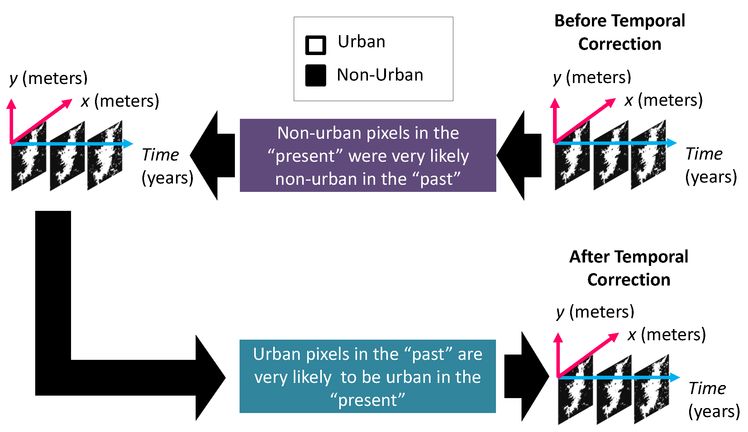
Figure 5.
Temporal interpolation of the population distribution.
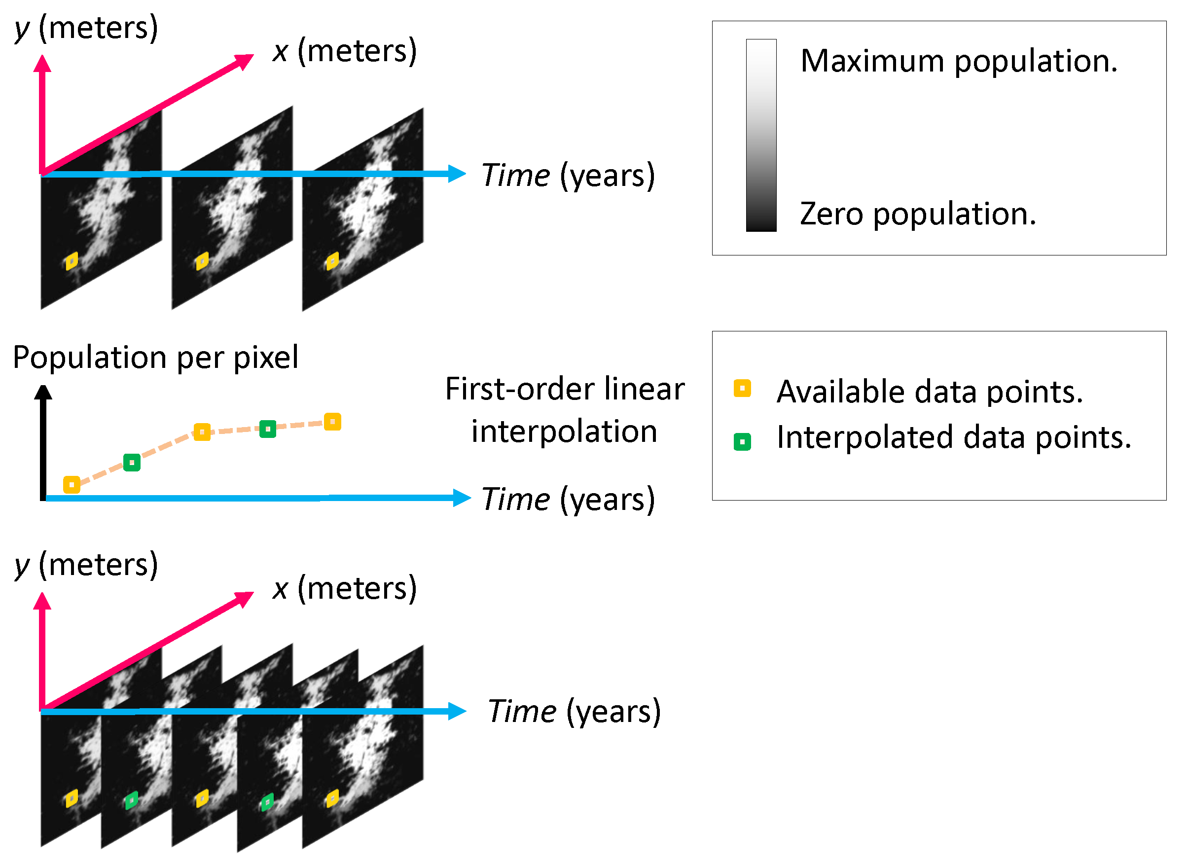
Figure 6.
Flow diagram with the harmonization process of the binary urban footprint using the population distribution. It has three main sub-processes that have been color-coded. The first sub-process finds the optimal threshold after which an area is considered urban. The second sub-process estimates the binary urban footprint for missing years using available information, a temporal correction, and the optimal threshold. The third sub-process cleans the binary urban footprint and only leaves urban pixels that are likely to be part of a city.
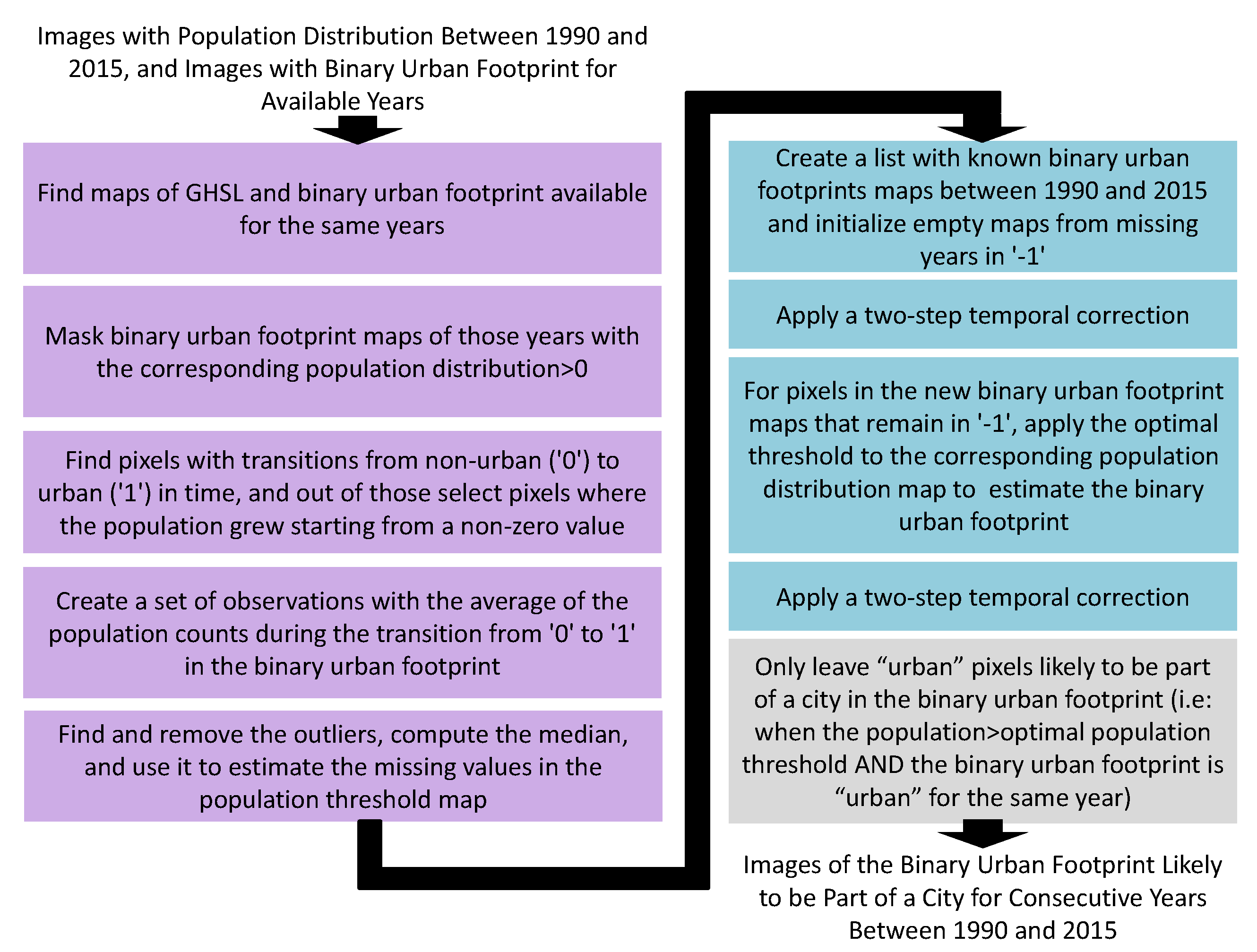
Figure 7.
Interaction among the three key variables of the urban growth framework: population distribution, binary urban footprint, and urban footprint.
Figure 7.
Interaction among the three key variables of the urban growth framework: population distribution, binary urban footprint, and urban footprint.

Figure 8.
Example of required data for modeling a multiple input single output spatio-temporal dynamic system of a selected city, assuming a temporal lag of two years for the input variables, and selecting the population distribution as the output variable. These data can be seen as part of a single temporal window of a larger dataset.
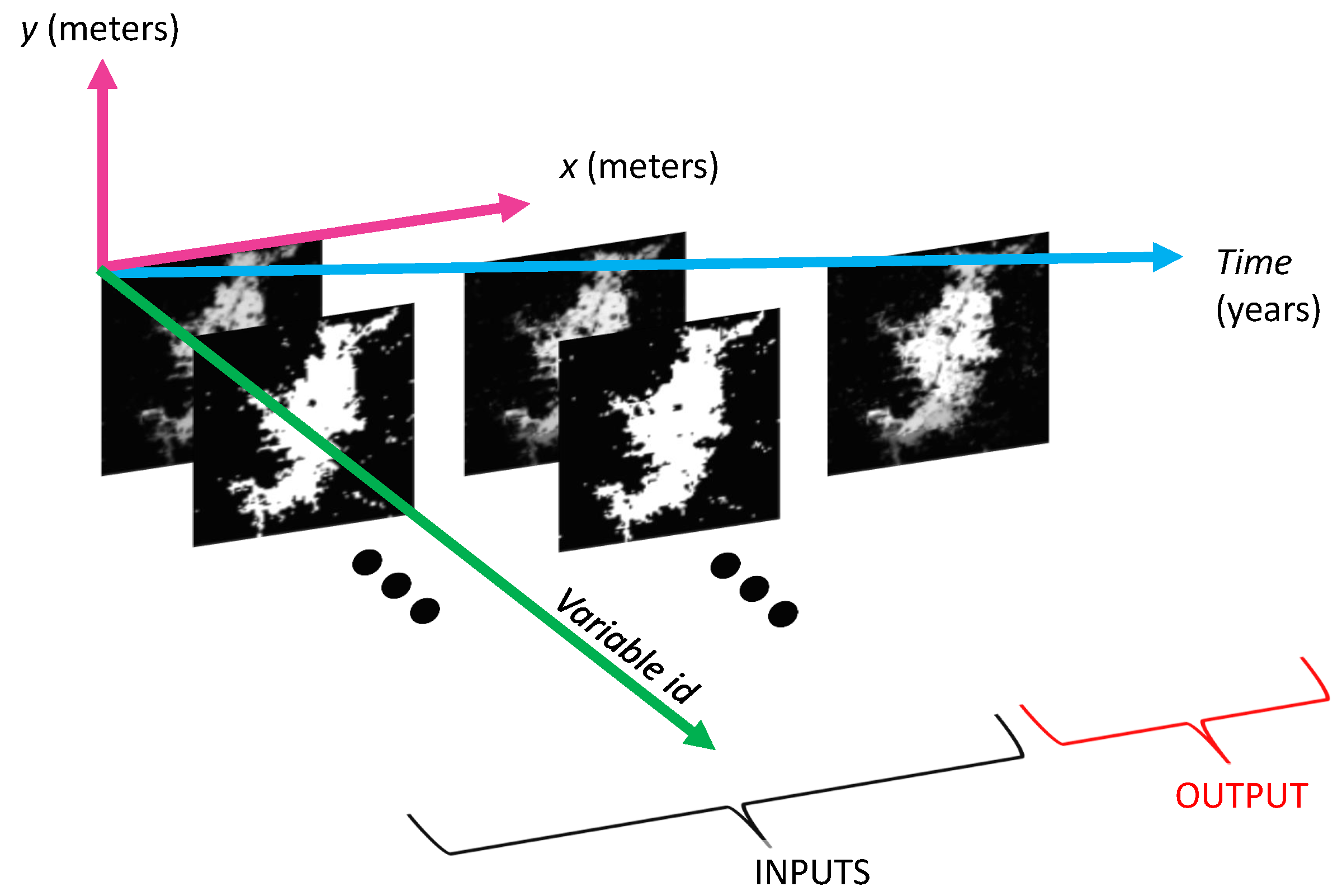
Figure 9.
Automated training, validation, and testing of the regression model to estimate the population distribution.
Figure 9.
Automated training, validation, and testing of the regression model to estimate the population distribution.

Figure 10.
Autotuning algorithm.
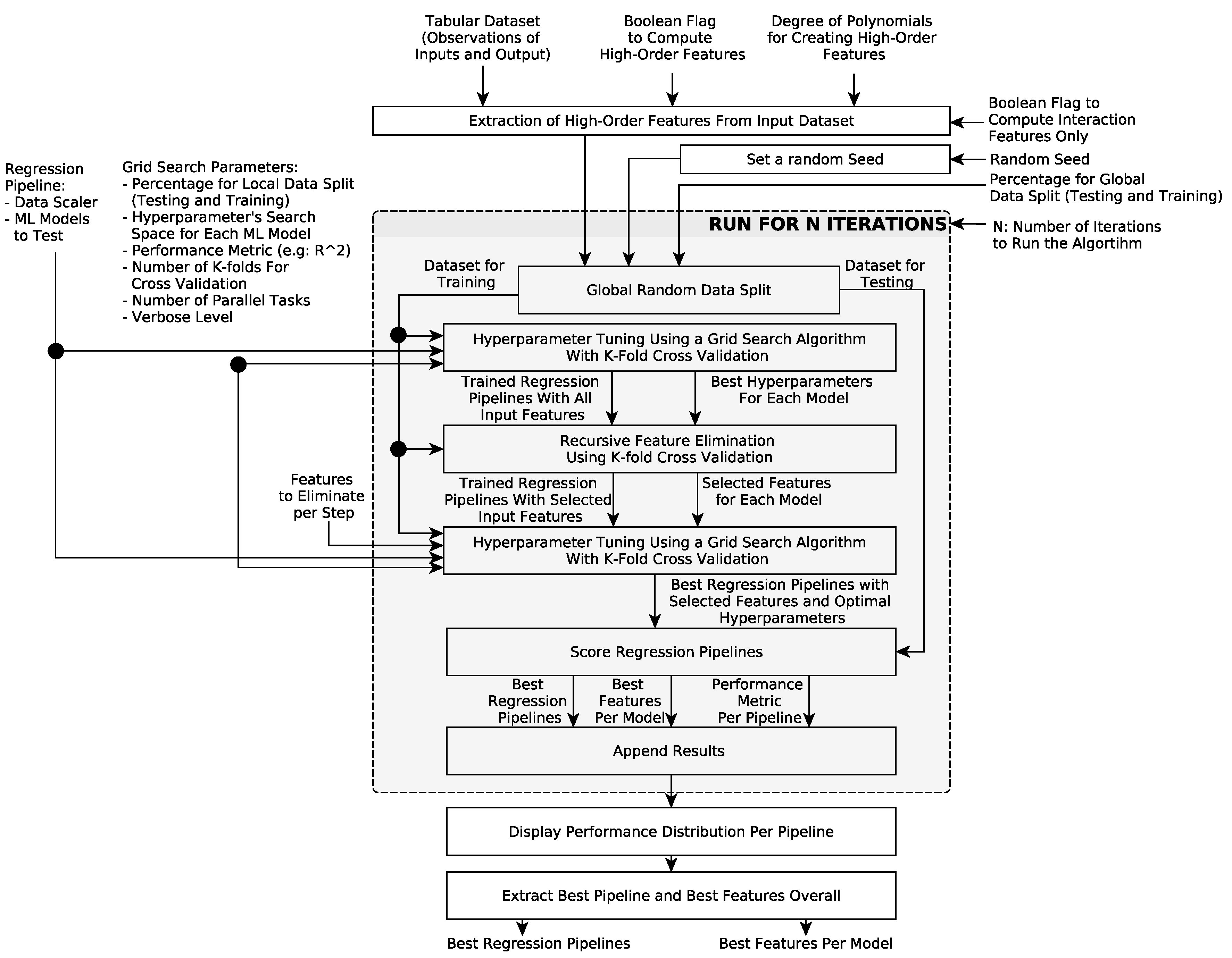
Figure 11.
Tested functions for saturating the predicted population given a maximum population capacity.
Figure 11.
Tested functions for saturating the predicted population given a maximum population capacity.
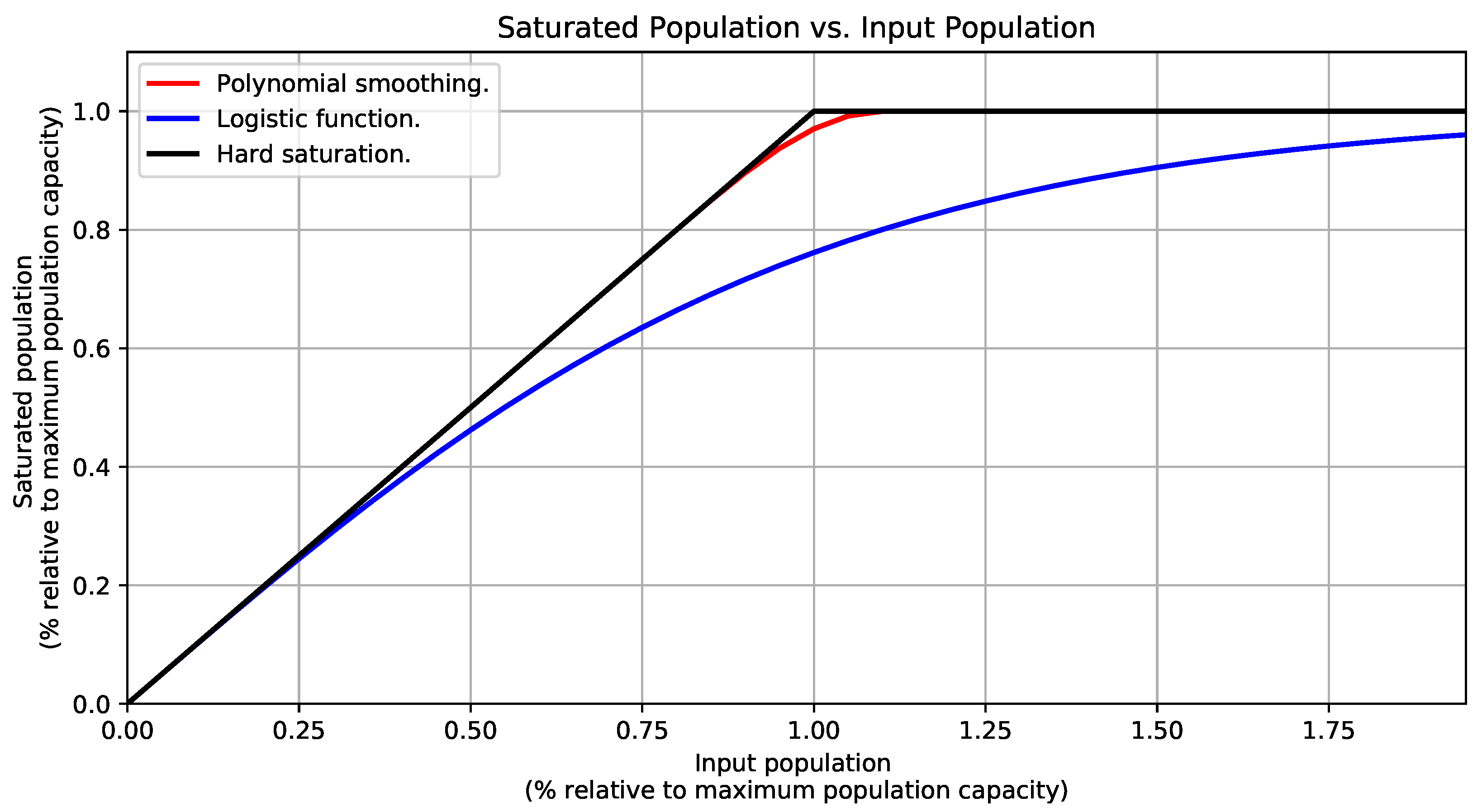
Figure 12.
Converting population distribution predictions into estimates of binary urban footprint during inference.
Figure 12.
Converting population distribution predictions into estimates of binary urban footprint during inference.

Figure 13.
Semantic inpainting to estimate the urban footprint in color at a final time from the value at an initial time and the the binary urban footprints at the initial and final times.
Figure 13.
Semantic inpainting to estimate the urban footprint in color at a final time from the value at an initial time and the the binary urban footprints at the initial and final times.
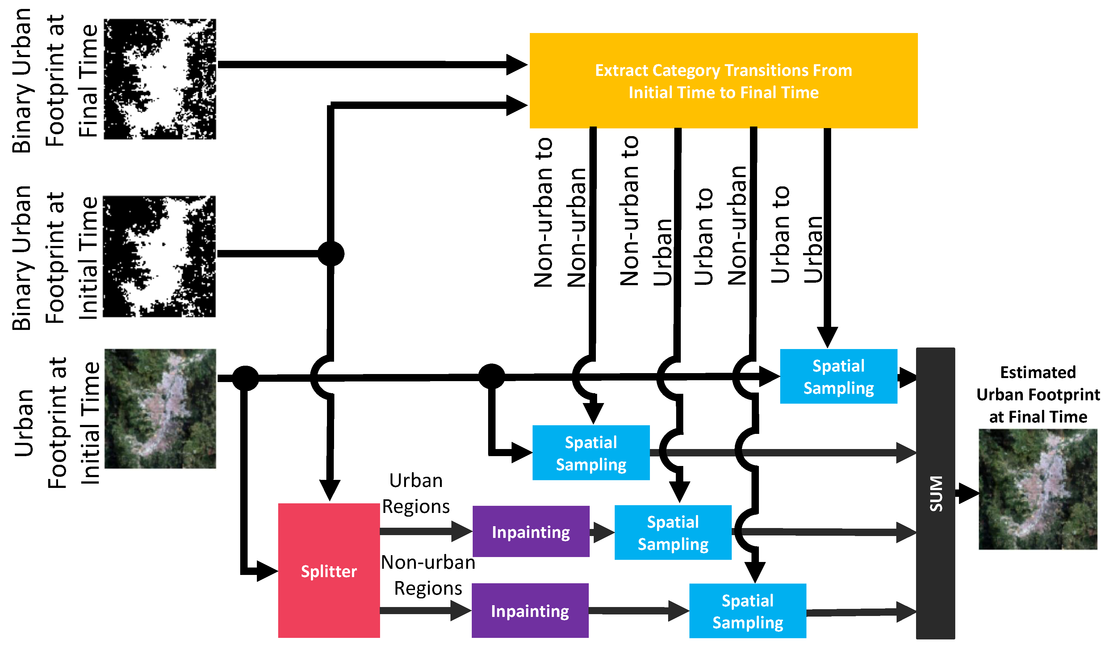
Figure 14.
Left: location of Valledupar and Rionegro in Colombia. Right: administrative divisions within the selected geographic extents for Valledupar and Rionegro.
Figure 14.
Left: location of Valledupar and Rionegro in Colombia. Right: administrative divisions within the selected geographic extents for Valledupar and Rionegro.
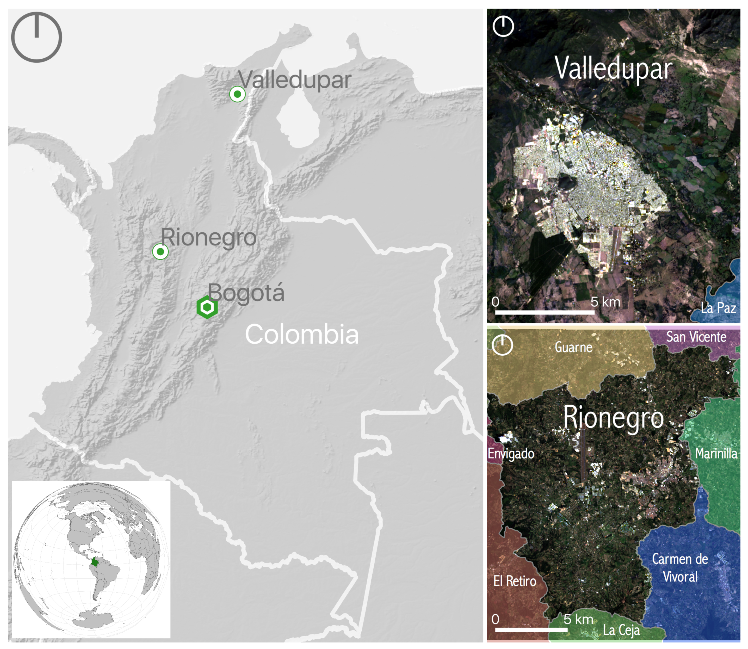
Figure 15.
Results of the classification process of Landsat images of Valledupar and Rionegro into urban and non-urban areas for the year 2015. The yellow regions highlight the urban classification results.
Figure 15.
Results of the classification process of Landsat images of Valledupar and Rionegro into urban and non-urban areas for the year 2015. The yellow regions highlight the urban classification results.
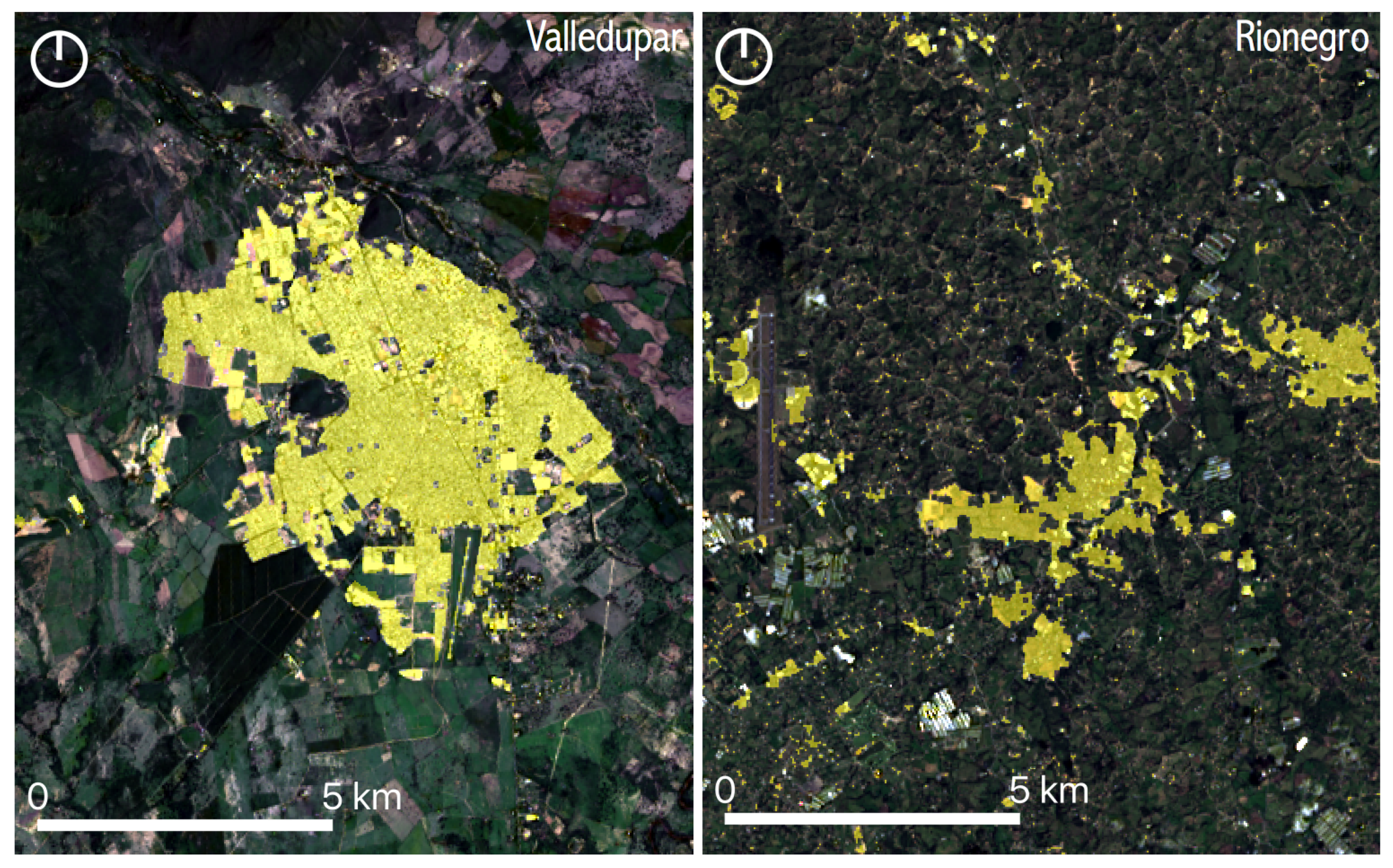
Figure 16.
Estimated probability density function of a population threshold after which a non-urban pixel becomes urban in Valledupar.
Figure 16.
Estimated probability density function of a population threshold after which a non-urban pixel becomes urban in Valledupar.

Figure 17.
Estimated probability density function of a population threshold after which a non-urban pixel becomes urban in Rionegro.
Figure 17.
Estimated probability density function of a population threshold after which a non-urban pixel becomes urban in Rionegro.

Figure 18.
Maps with population thresholds beyond which non-urban pixels become urban.
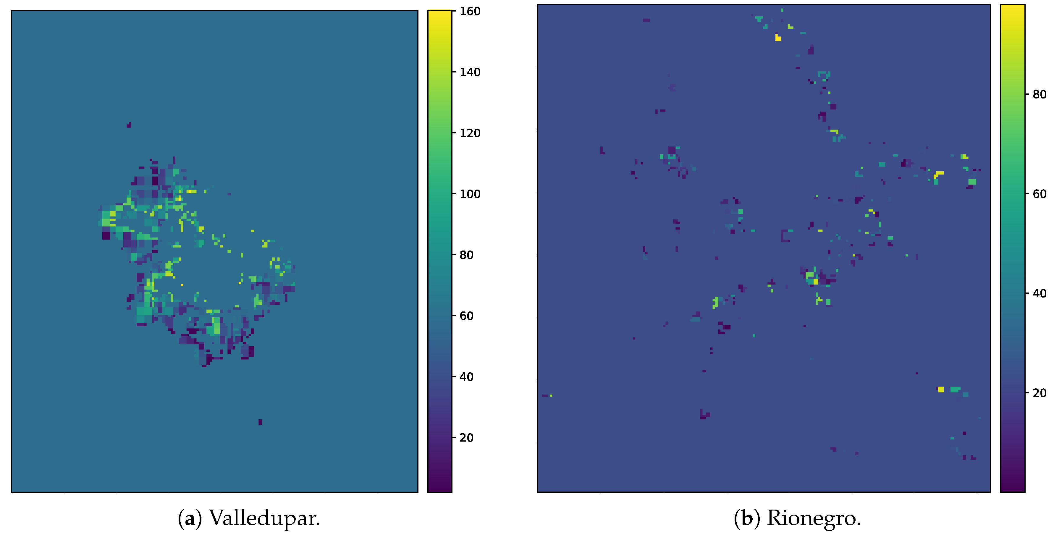
Figure 19.
Diagnostic graphs of the geographic area of interest masked by the administrative division of Valledupar. (Left) total urban population. (Center) total urban area. (Right) urban density.
Figure 19.
Diagnostic graphs of the geographic area of interest masked by the administrative division of Valledupar. (Left) total urban population. (Center) total urban area. (Right) urban density.

Figure 20.
Diagnostic graphs of the geographic area of interest masked by the administrative division of Rionegro. (Left) total urban population. (Center) total urban area. (Right) urban density.
Figure 20.
Diagnostic graphs of the geographic area of interest masked by the administrative division of Rionegro. (Left) total urban population. (Center) total urban area. (Right) urban density.
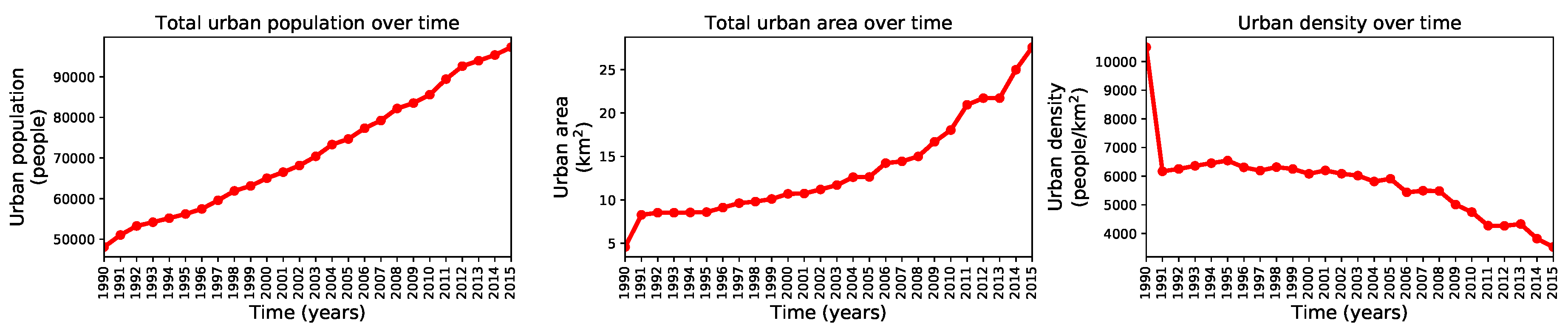
Figure 21.
Estimated probability density functions of the mean square error in the spatiotemporal regression of the population distribution for different families of models as returned by the autotuning program in Valledupar.
Figure 21.
Estimated probability density functions of the mean square error in the spatiotemporal regression of the population distribution for different families of models as returned by the autotuning program in Valledupar.
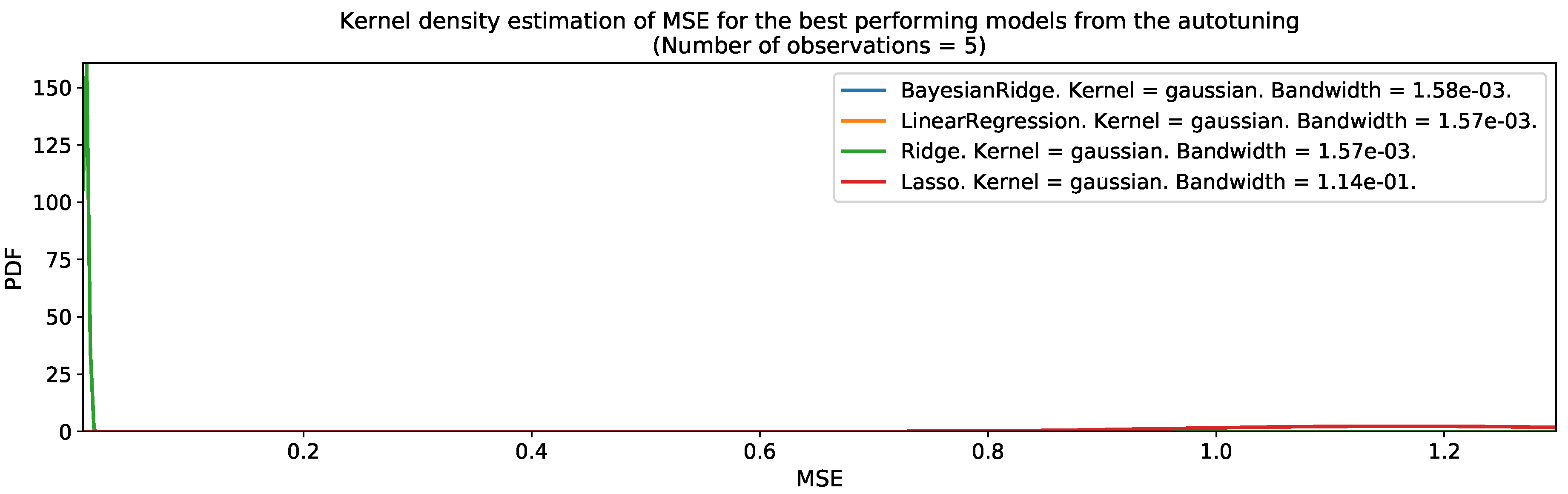
Figure 22.
Estimated probability density functions of the mean square error in the spatiotemporal regression of the population distribution for different families of models as returned by the autotuning program in Rionegro.
Figure 22.
Estimated probability density functions of the mean square error in the spatiotemporal regression of the population distribution for different families of models as returned by the autotuning program in Rionegro.

Figure 23.
Framework performance in the geographic areas of interest. From left to right, the columns correspond to: (1) population distribution error (i.e., real value - predicted value); (2) histogram of the population distribution error; (3) binary urban footprint error (i.e., real value - predicted value); (4) histogram of the binary urban footprint error. POP = predicted population distributions; BUF = binary urban footprints; ZNCC = zero-mean normalized cross-correlation; SAD = sum of absolute differences; SSD = sum of squared differences.

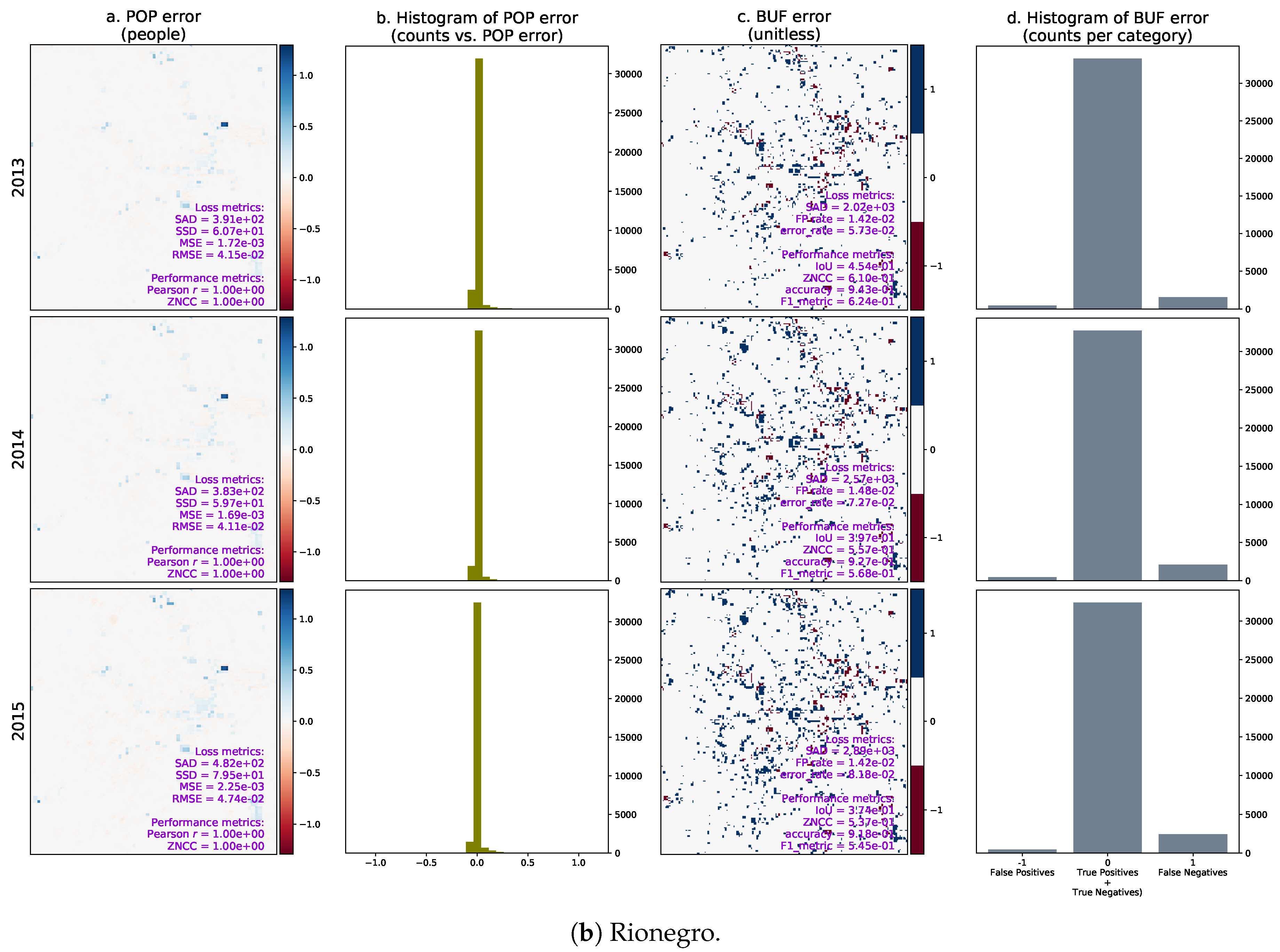
Figure 24.
Assessment of the urban predictions in the geographic area of interest masked by the administrative division of Valledupar with the test set.
Figure 24.
Assessment of the urban predictions in the geographic area of interest masked by the administrative division of Valledupar with the test set.

Figure 25.
Assessment of the urban predictions in the geographic area of interest masked by the administrative division of Rionegro with the test set.
Figure 25.
Assessment of the urban predictions in the geographic area of interest masked by the administrative division of Rionegro with the test set.
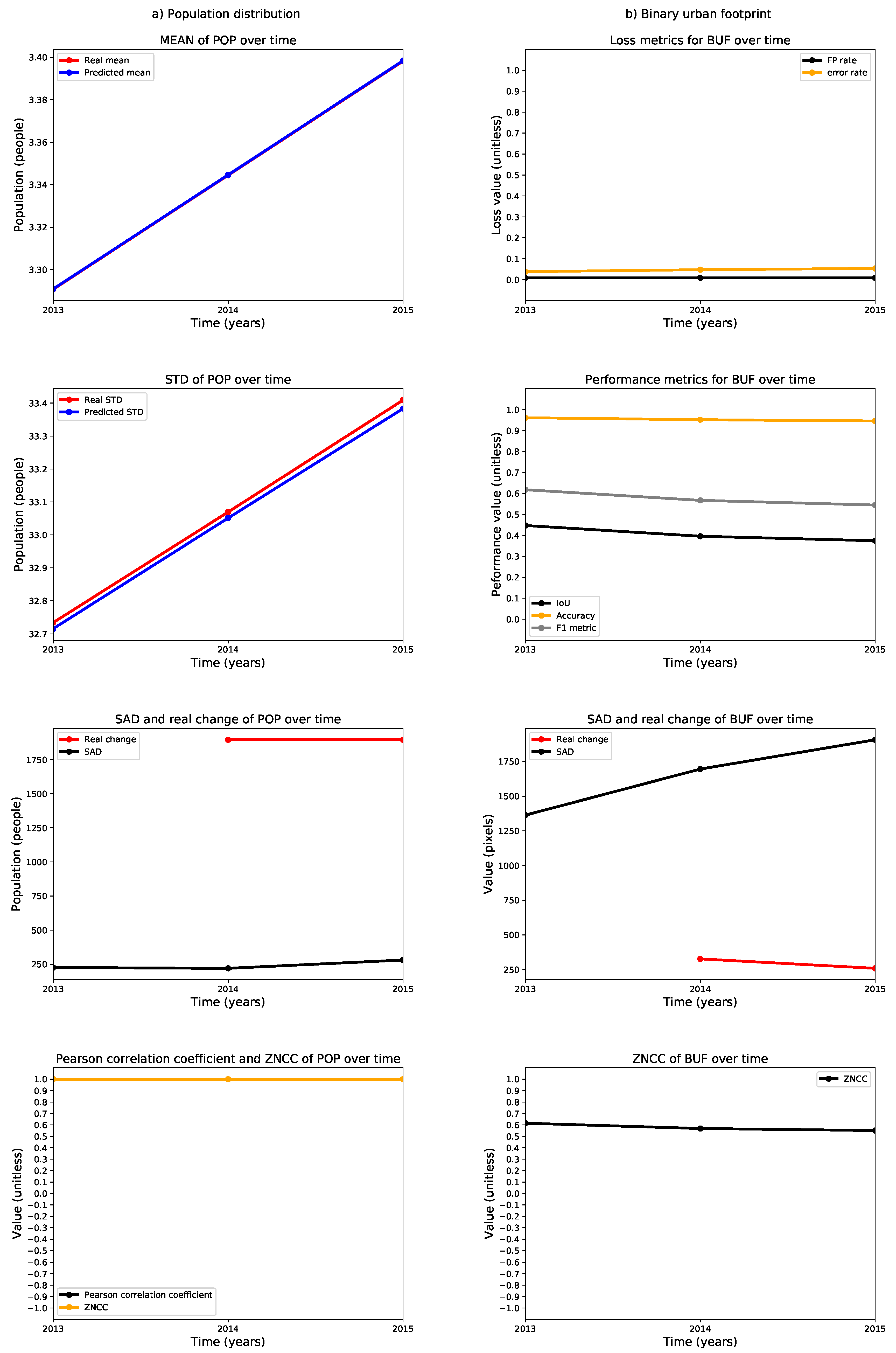
Figure 26.
Urban growth predictions in the geographic area of interest that includes Valledupar.
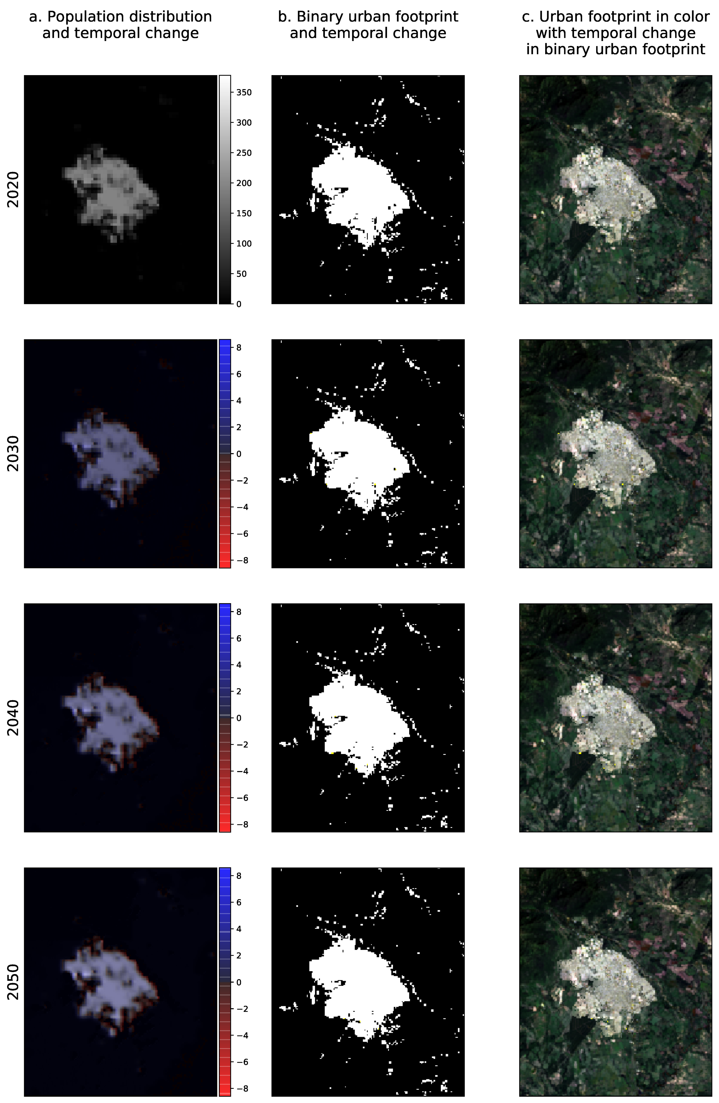
Figure 27.
Urban growth predictions in the geographic area of interest that includes Rionegro.


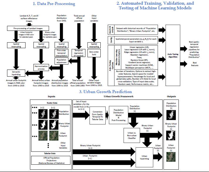
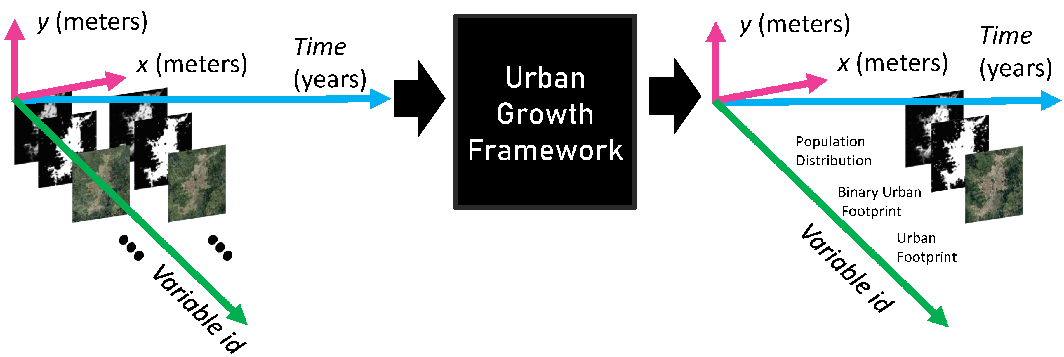
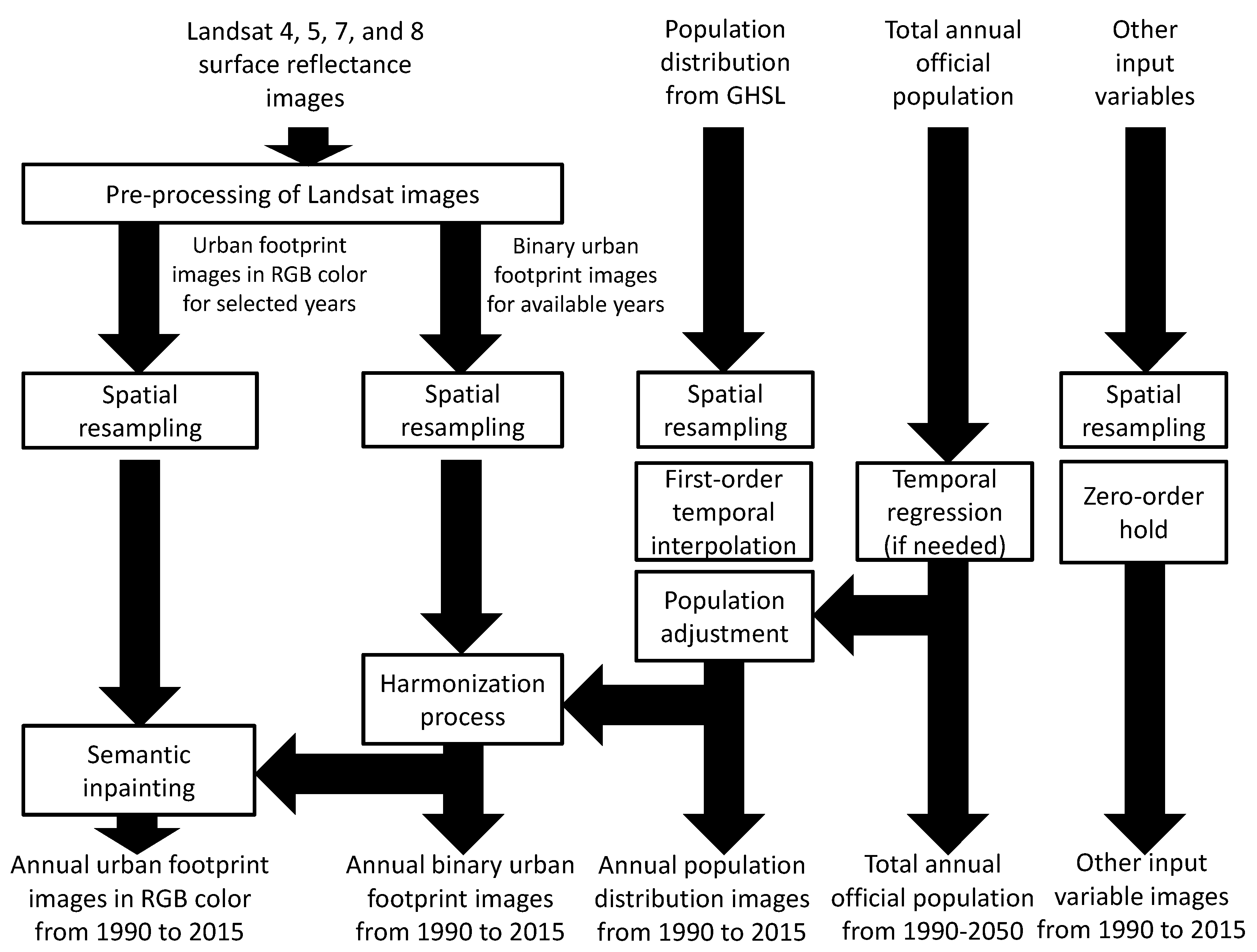
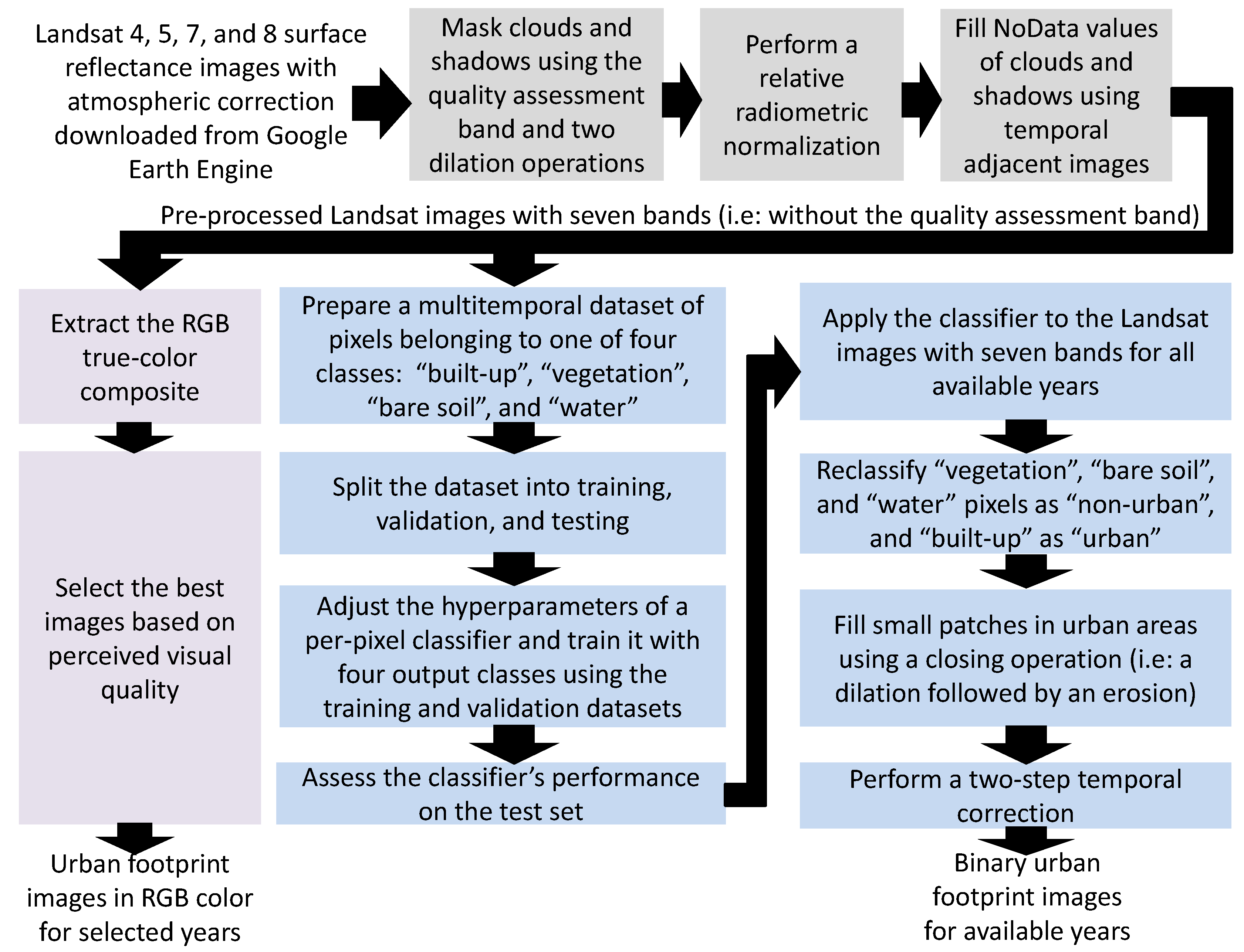
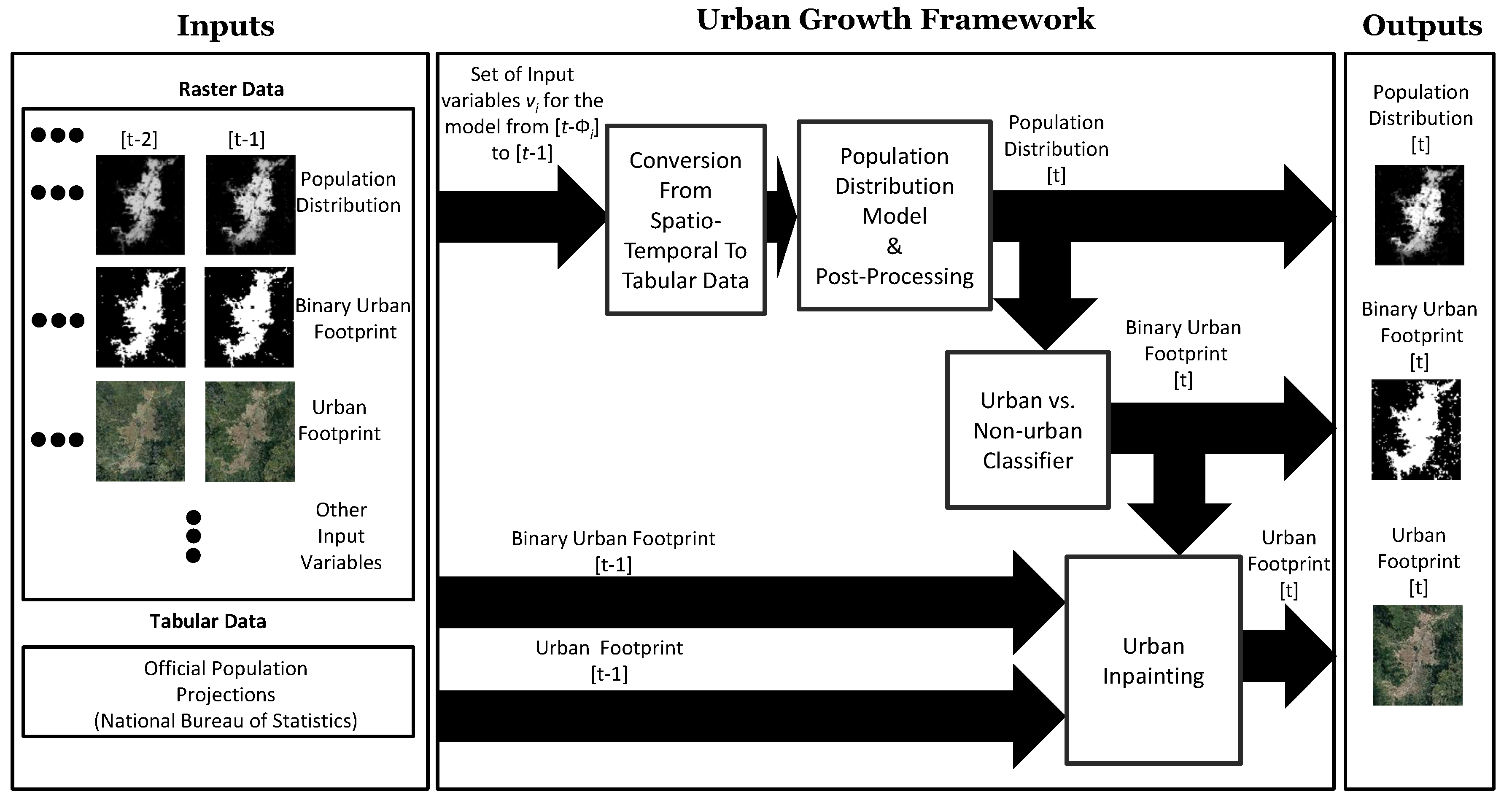
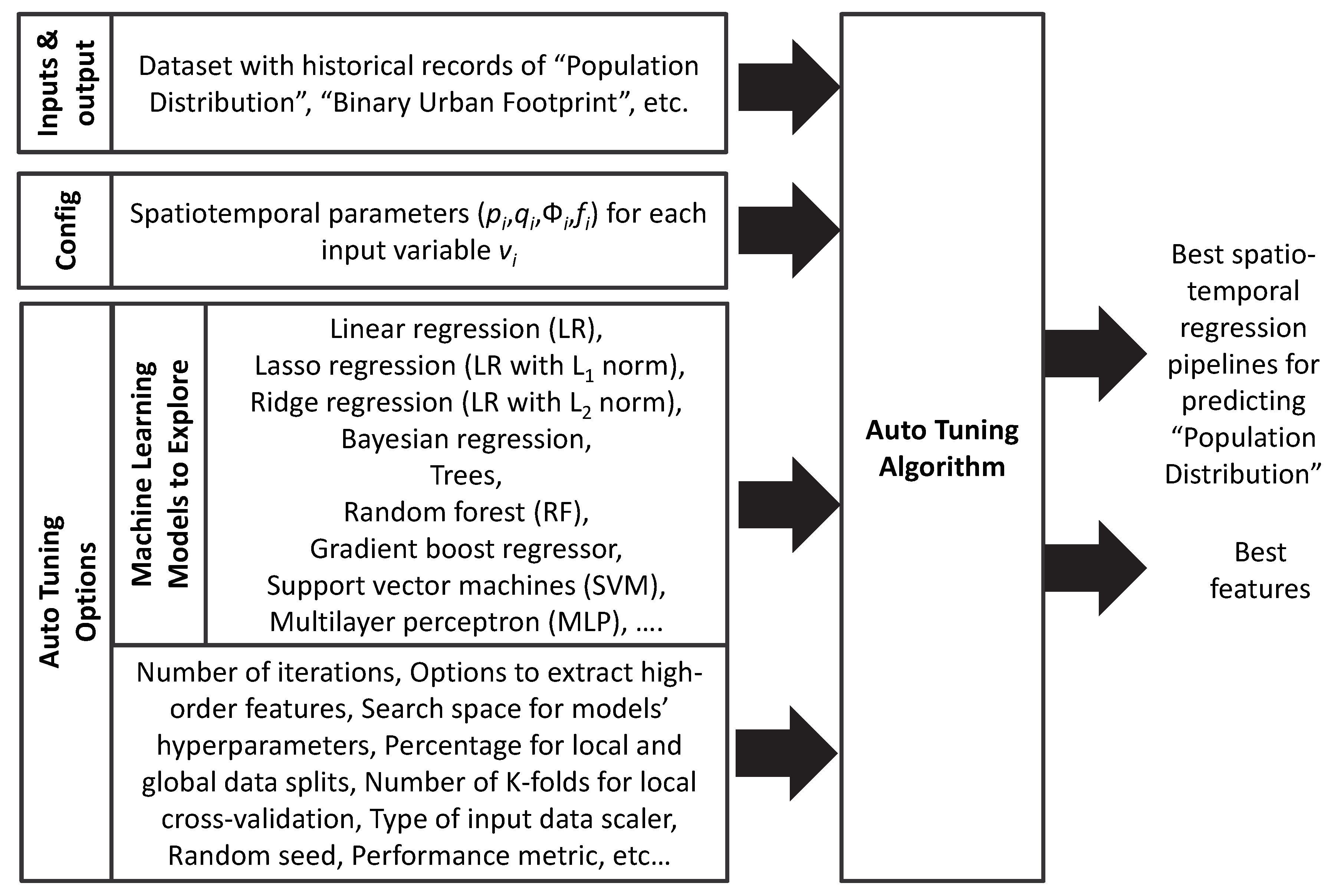
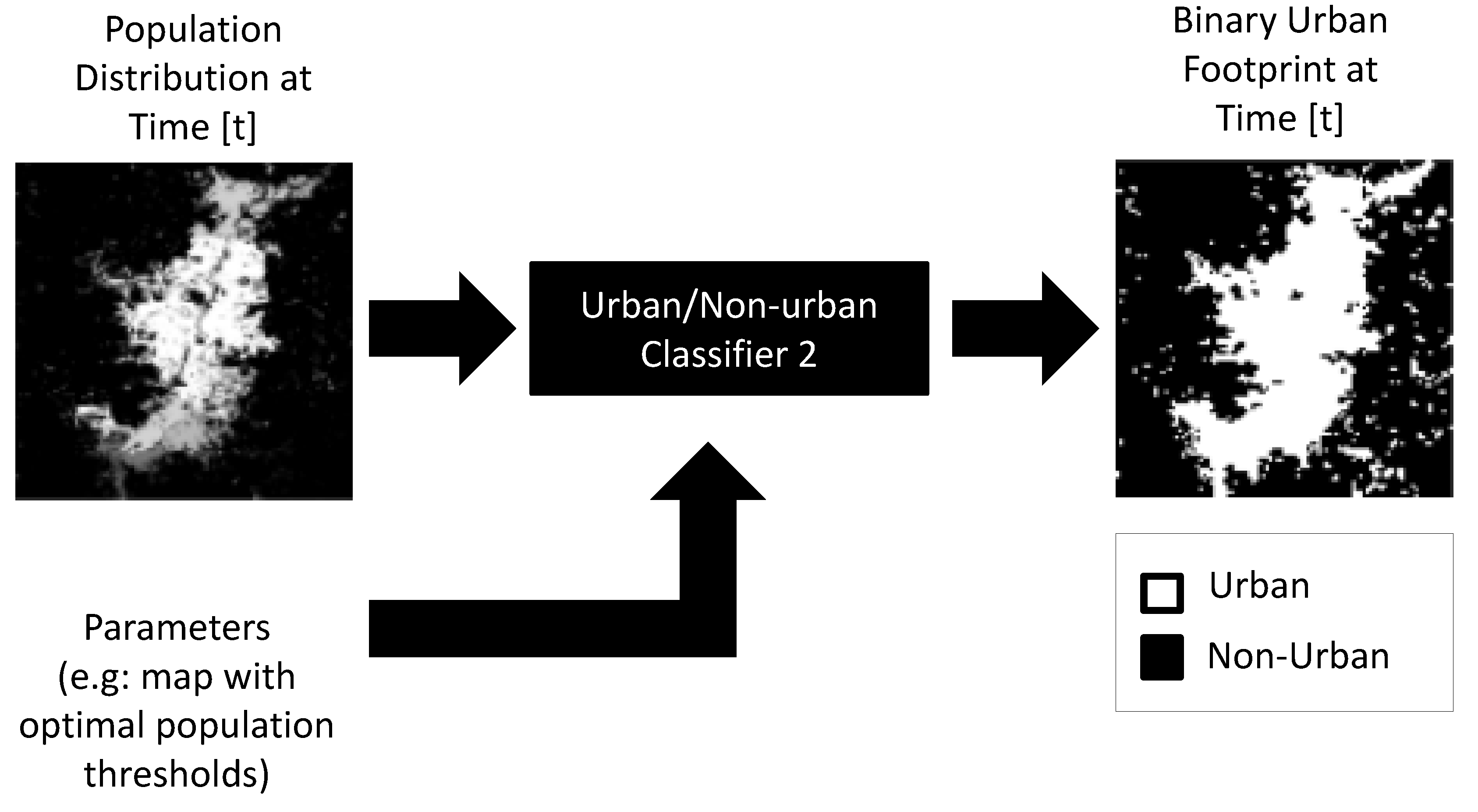
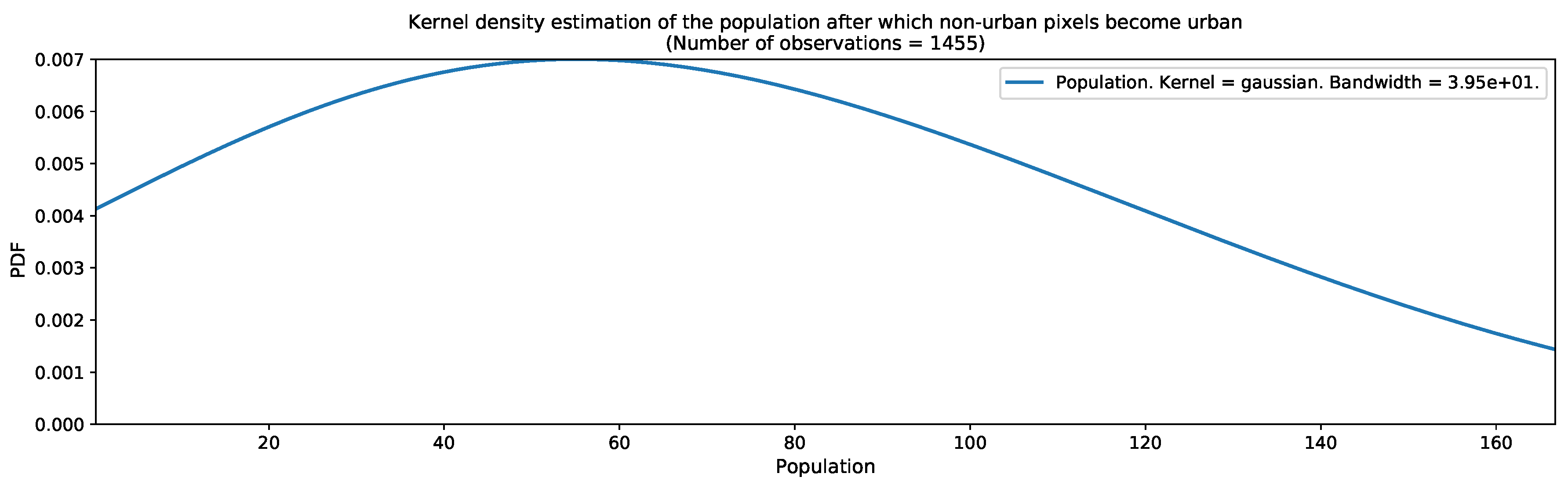
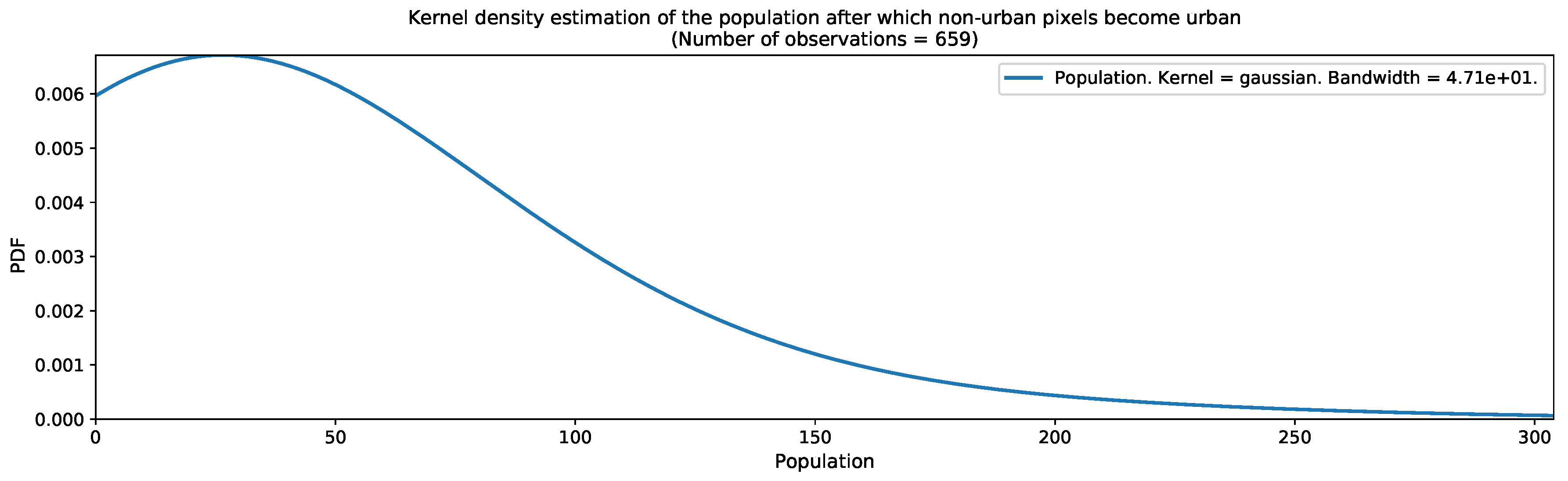
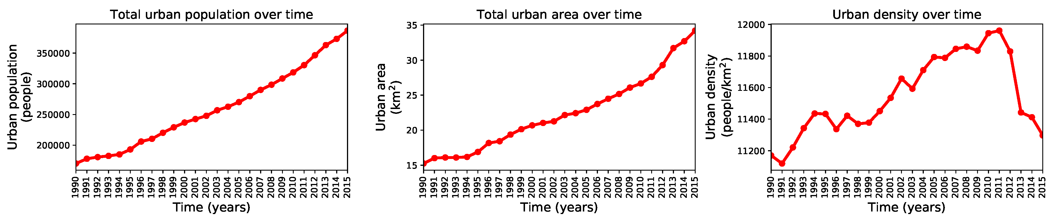
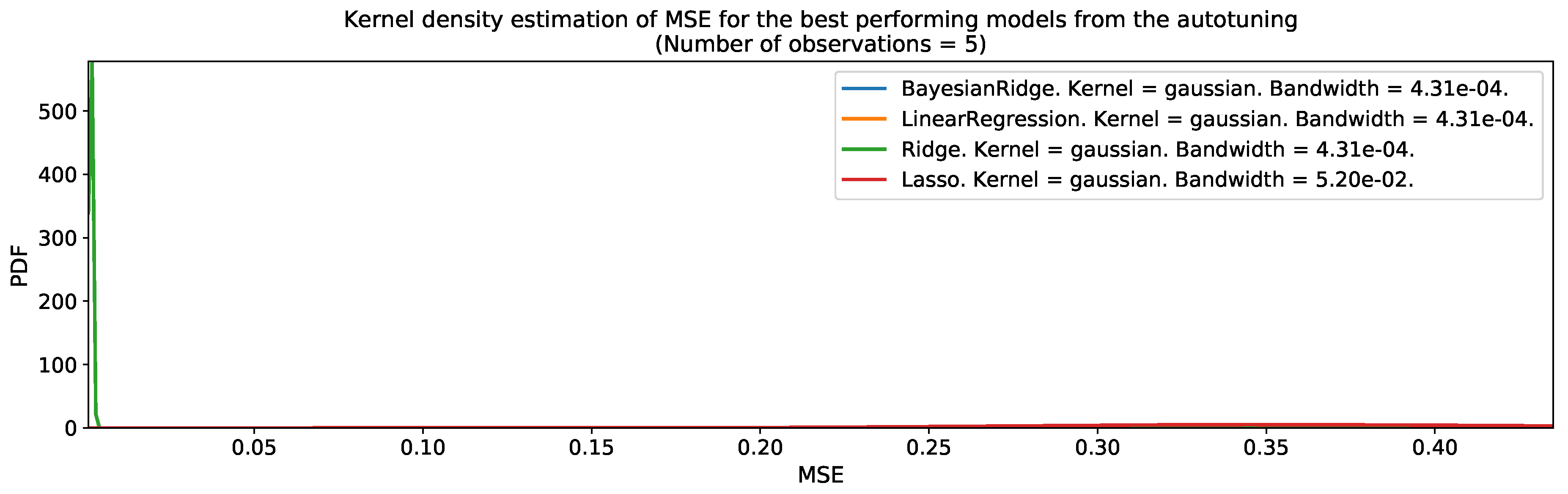
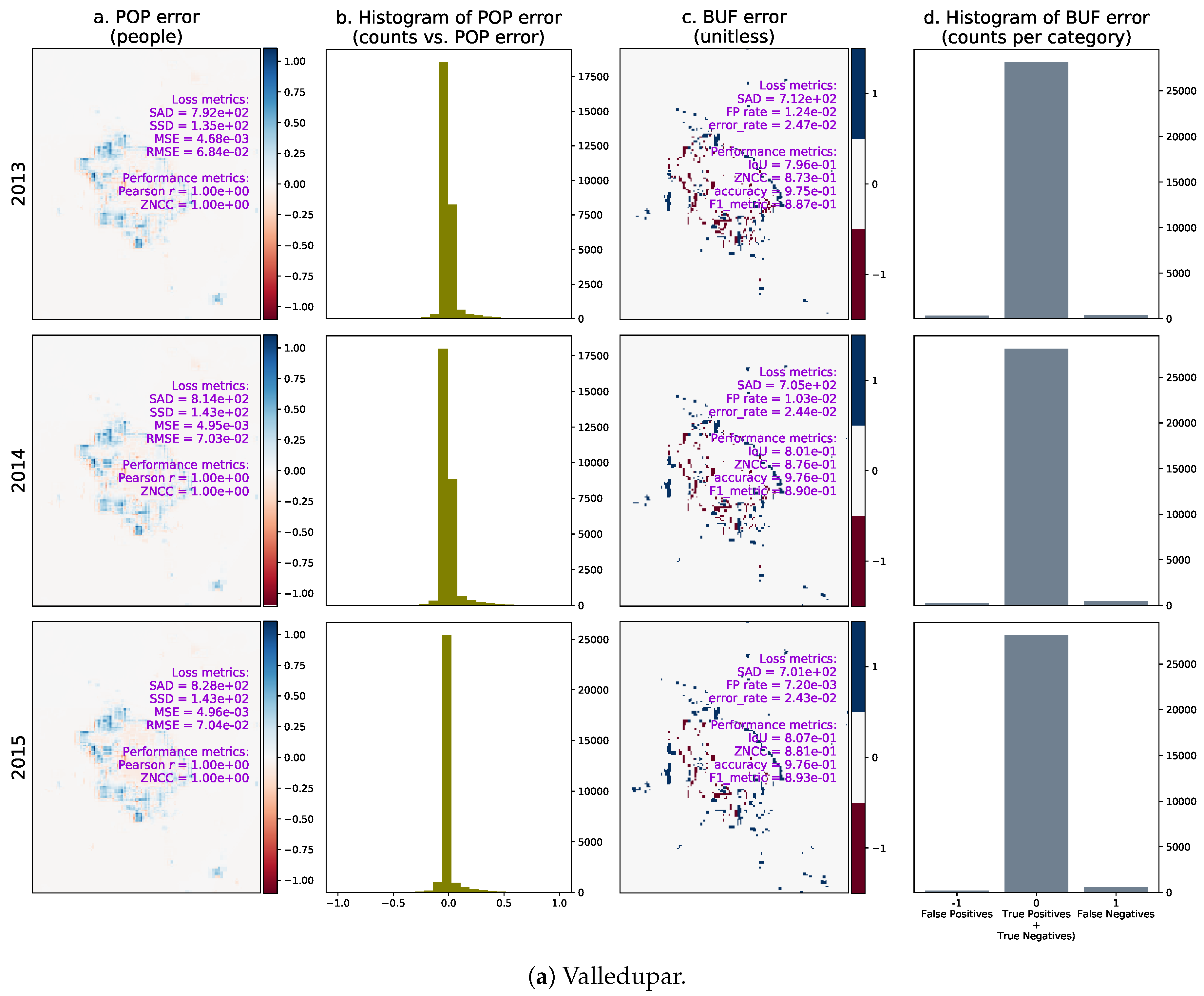
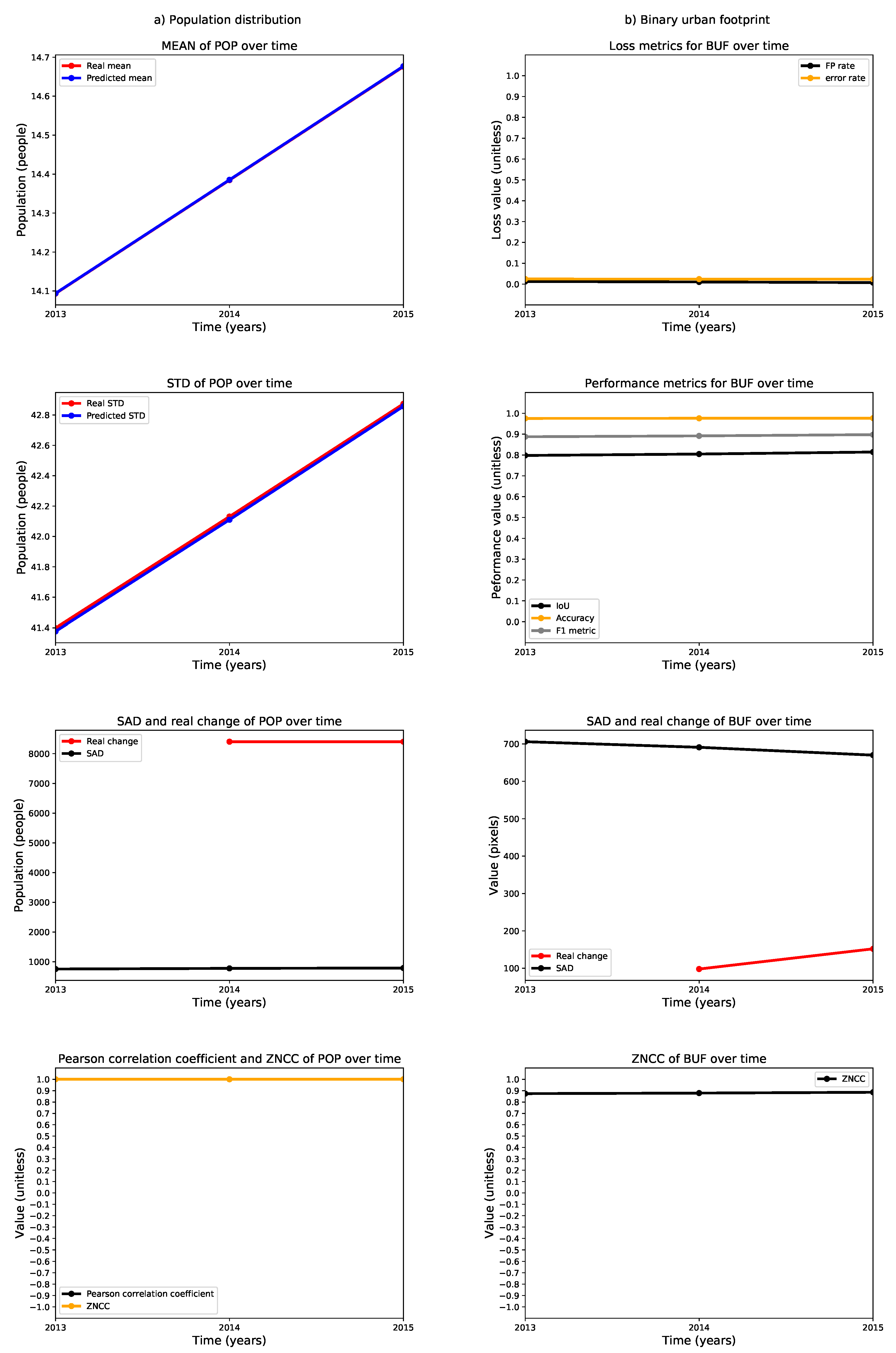
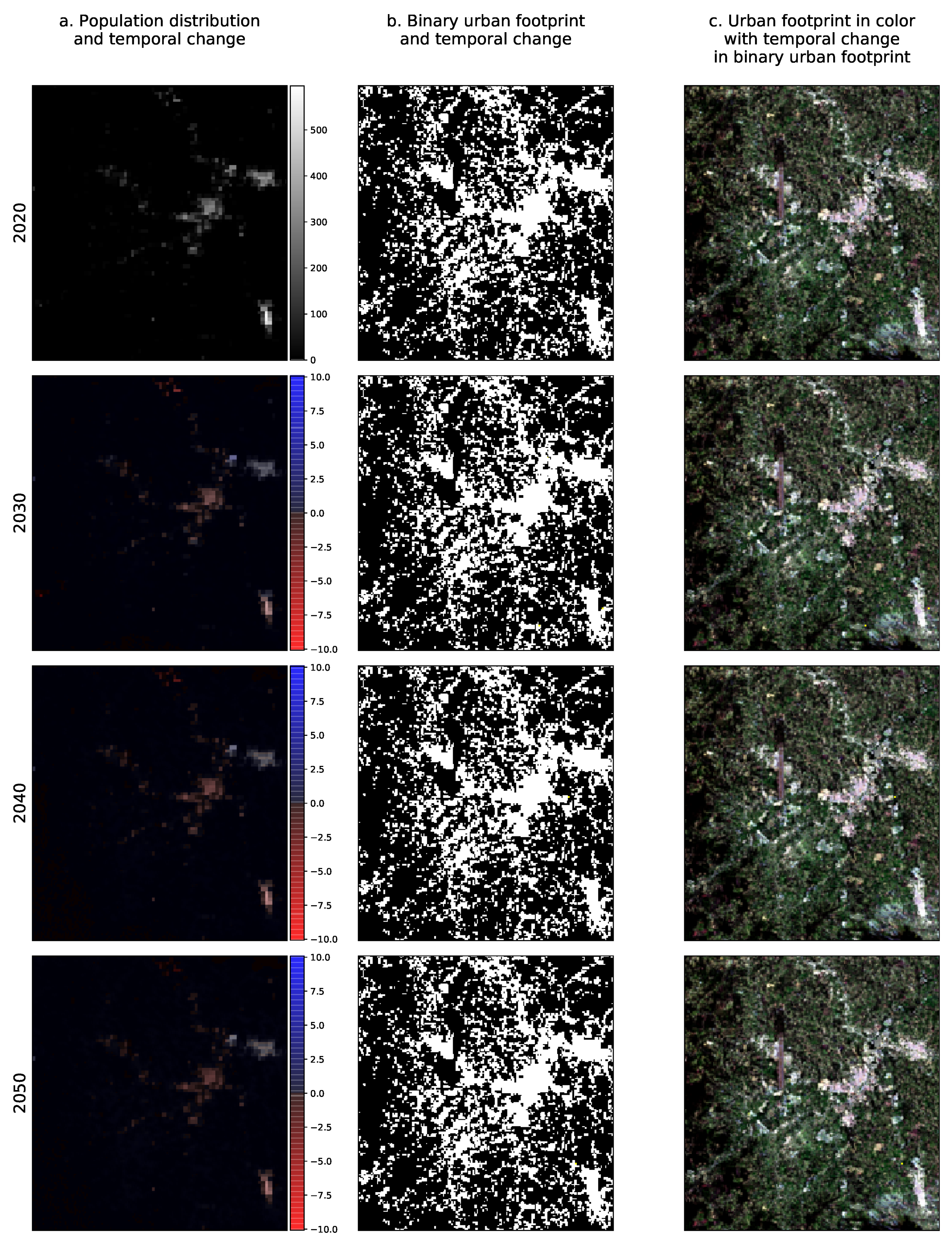
Table 1.
Examples of variables that the urban-growth framework can handle. GHSL = Global Human Settlement Layer; SRTM = Shuttle Radar Topography Mission; OSM = Open Street Map; IGAC = Agustín Codazzi Geographic Institute; WDPA = World Database on Protected Areas.
Table 1.
Examples of variables that the urban-growth framework can handle. GHSL = Global Human Settlement Layer; SRTM = Shuttle Radar Topography Mission; OSM = Open Street Map; IGAC = Agustín Codazzi Geographic Institute; WDPA = World Database on Protected Areas.
| Variable Name | Data Source | Digital Format | Resolution | Availability | Importance |
|---|---|---|---|---|---|
| Population distribution. | GHSL pop [45]. | Raster. | 250 m × 250 m. | Global. | Essential. |
| Urban footprint. | Landsat [47]. | Raster. | 30 m × 30 m. | Global. | Essential. |
| Binary urban footprint. | Derived from the urban footprint through a binary classifier. | Raster. | 30 m × 30 m. | Global. | Essential. |
| Official population projections. | National Bureau of Statistics [48]. | Tabular. | Administrative units. | National. | Optional. |
| Maximum population capacity. | Master plan [49,50]. | Vector. | - | Local. | Optional. |
| Land use (residential, industrial, commercial, official, and special). | Master plan [49,50]. | Vector. | - | Local. | Optional. |
| Built-up urban ratio. | GHSL built-up [51]. | Raster. | 250 m × 250 m. | Global. | Optional. |
| Terrain slope. | SRTM [52]. | Raster. | 90 m × 90 m. | Global. | Optional. |
| Distances to nearest populated towns. | Derived from binary urban footprint. | Raster. | 30 m × 30 m. | Global. | Optional. |
| Roads. | OSM [53], IGAC [54]. | Vector. | - | Global, National. | Optional. |
| Natural hazard (flooding, landslide, fire, volcanic eruption, earthquake.). | Master plan [49,50]. | Vector. | - | Local. | Optional. |
| Water bodies. | Master plan [49,50], IGAC [54]. | Vector. | - | Local. | Optional. |
| Protected areas. | Master plan [49,50], WDPA [55]. | Vector. | - | Global, Local. | Optional. |
| Urban development projects. | Master plan [49,50], others. | Vector. | - | Local. | Optional. |
Table 2.
Terminology of the urban growth framework.
| Variables | Description |
|---|---|
| t | Time in years. |
| r | Number of consecutive years of historical data records available for training. |
| Spatial coordinates along the East and North directions, respectively. | |
| Width and height of the spatial extent under study in meters. | |
| Spatial sampling period in meters along the x and y directions, respectively. | |
| Number of rows and columns of each digital image. | |
| Auxiliary variables. | |
| Population distribution. | |
| Binary urban footprint (black and white). | |
| Urban footprint (color). | |
| i-th input variable. | |
| Number of rows and columns of the spatial window for . | |
| Number of consecutive temporal lags in years for . | |
| Mathematical function applied to each possible spatial window of pixels in . In the naïve feature sampling, it corresponds to a reshape operation to convert the data dimensions from to . In other scenarios it can be a spatial-filtering function that processes and reduces the number of features (e.g., an element-wise multiplication of the spatial window by a fixed spatial kernel of the same dimensions followed by a sum of its elements). | |
| Number of temporal windows that can be extracted from the historical data records for all variables given the maximum consecutive temporal lag in the regression model. | |
| Number of rows (i.e., observations) and columns (i.e., input features) of the resulting tabular dataset for training the population distribution growth model based on machine learning. | |
| Population threshold after which a region can be considered as urbanized. |
Table 3.
Confusion matrices for the classification process of Landsat images in Valledupar. The top table corresponds to the initial classification process of pixels into four categories, and the bottom table corresponds to the final re-classification process into two categories.
Table 3.
Confusion matrices for the classification process of Landsat images in Valledupar. The top table corresponds to the initial classification process of pixels into four categories, and the bottom table corresponds to the final re-classification process into two categories.
| Predicted Class | |||||
|---|---|---|---|---|---|
| built-up | bare soil | vegetation | water | ||
| True class | built-up | 2094 | 45 | 3 | 0 |
| bare soil | 28 | 9339 | 7 | 0 | |
| vegetation | 0 | 24 | 17,504 | 6 | |
| water | 0 | 6 | 43 | 89 | |
| Predicted Class | |||||
| urban | non-urban | ||||
| True class | urban | 2094 | 48 | ||
| non-urban | 28 | 27,018 | |||
Table 4.
Confusion matrices for the classification process of Landsat images in Rionegro. The top table corresponds to the initial classification process of pixels into four categories and the bottom table corresponds to the final re-classification process into two categories.
Table 4.
Confusion matrices for the classification process of Landsat images in Rionegro. The top table corresponds to the initial classification process of pixels into four categories and the bottom table corresponds to the final re-classification process into two categories.
| Predicted Class | |||||
|---|---|---|---|---|---|
| built-up | bare soil | vegetation | water | ||
| True class | built-up | 1355 | 29 | 11 | 1 |
| bare soil | 61 | 535 | 15 | 1 | |
| vegetation | 0 | 10 | 5557 | 0 | |
| water | 1 | 7 | 3 | 73 | |
| Predicted Class | |||||
| urban | non-urban | ||||
| True class | urban | 1355 | 41 | ||
| non-urban | 62 | 6201 | |||
© 2019 by the authors. Licensee MDPI, Basel, Switzerland. This article is an open access article distributed under the terms and conditions of the Creative Commons Attribution (CC BY) license (http://creativecommons.org/licenses/by/4.0/).
Share and Cite
MDPI and ACS Style
Gómez, J.A.; Patiño, J.E.; Duque, J.C.; Passos, S. Spatiotemporal Modeling of Urban Growth Using Machine Learning. Remote Sens. 2020, 12, 109. https://doi.org/10.3390/rs12010109
AMA Style
Gómez JA, Patiño JE, Duque JC, Passos S. Spatiotemporal Modeling of Urban Growth Using Machine Learning. Remote Sensing. 2020; 12(1):109. https://doi.org/10.3390/rs12010109
Chicago/Turabian StyleGómez, Jairo A., Jorge E. Patiño, Juan C. Duque, and Santiago Passos. 2020. "Spatiotemporal Modeling of Urban Growth Using Machine Learning" Remote Sensing 12, no. 1: 109. https://doi.org/10.3390/rs12010109
Note that from the first issue of 2016, this journal uses article numbers instead of page numbers. See further details here.