Comparison of Aqua/Terra MODIS and Himawari-8 Satellite Data on Cloud Mask and Cloud Type Classification Using Split Window Algorithm

 ,
,
Abstract
:
1. Introduction
2. Methods
2.1. Band Selection
2.2. Cloud Masking
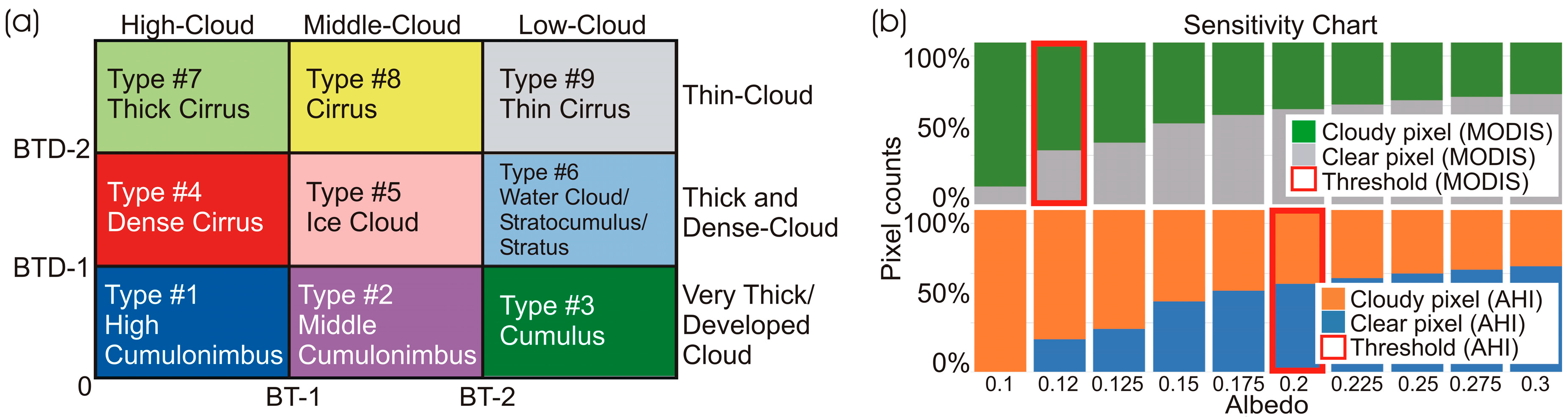
2.3. Cloud Classification
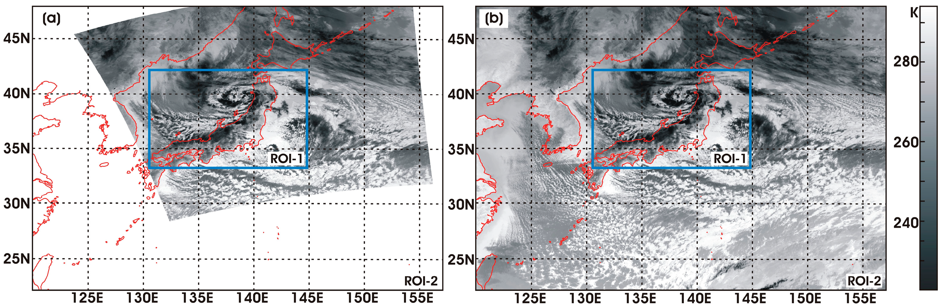
2.4. Validation
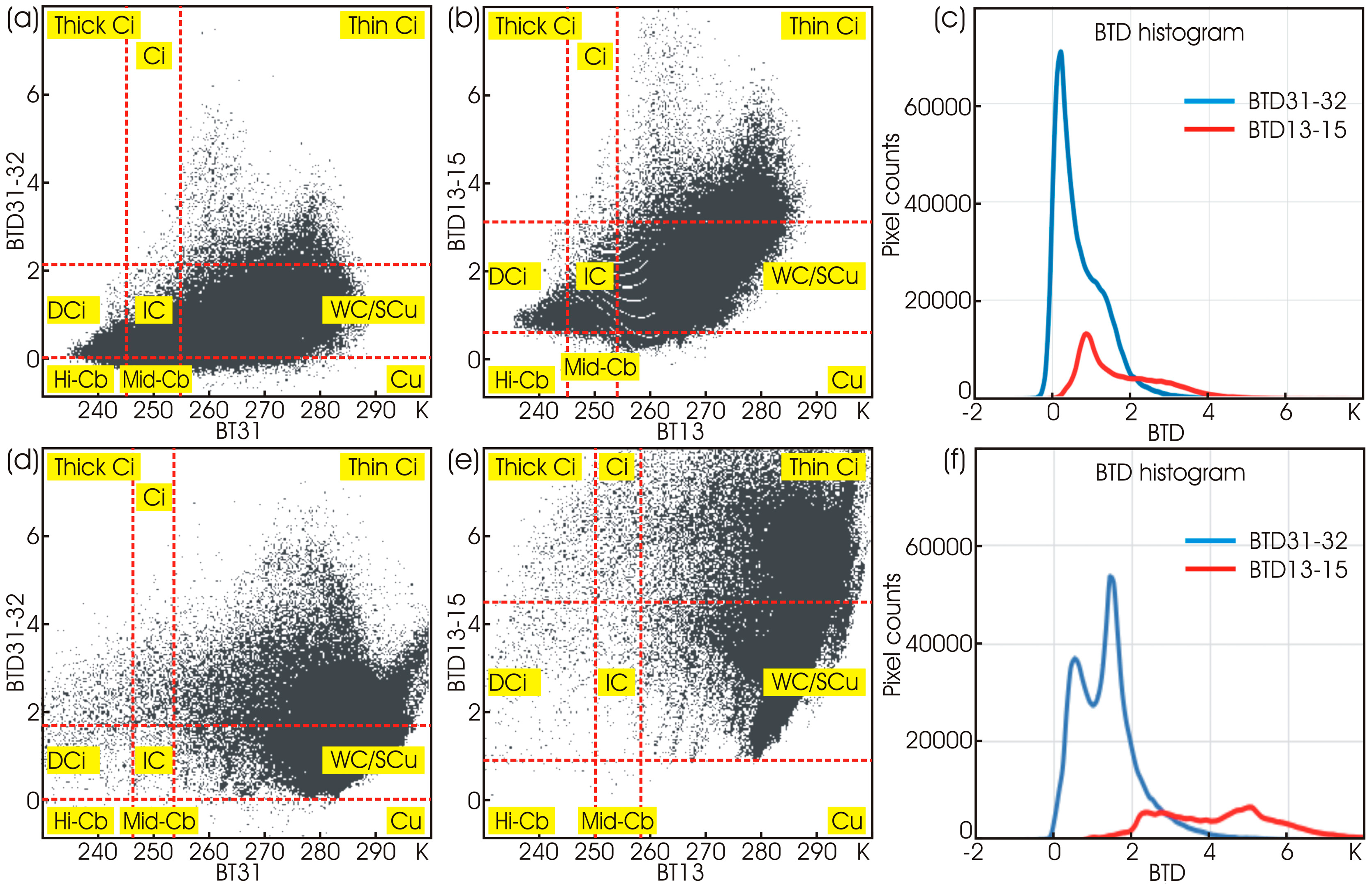
2.5. Determination of Thresholds
3. Results
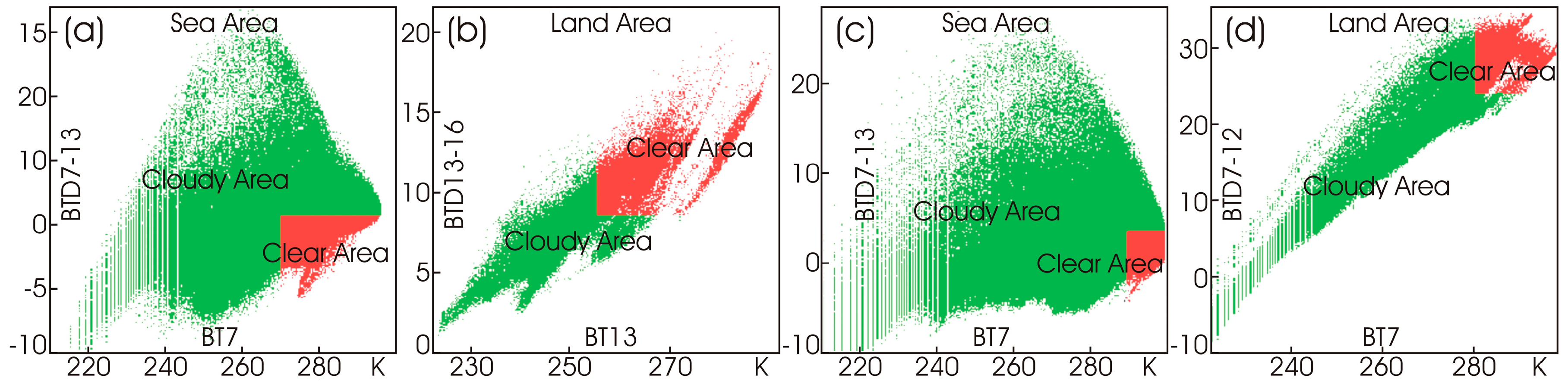
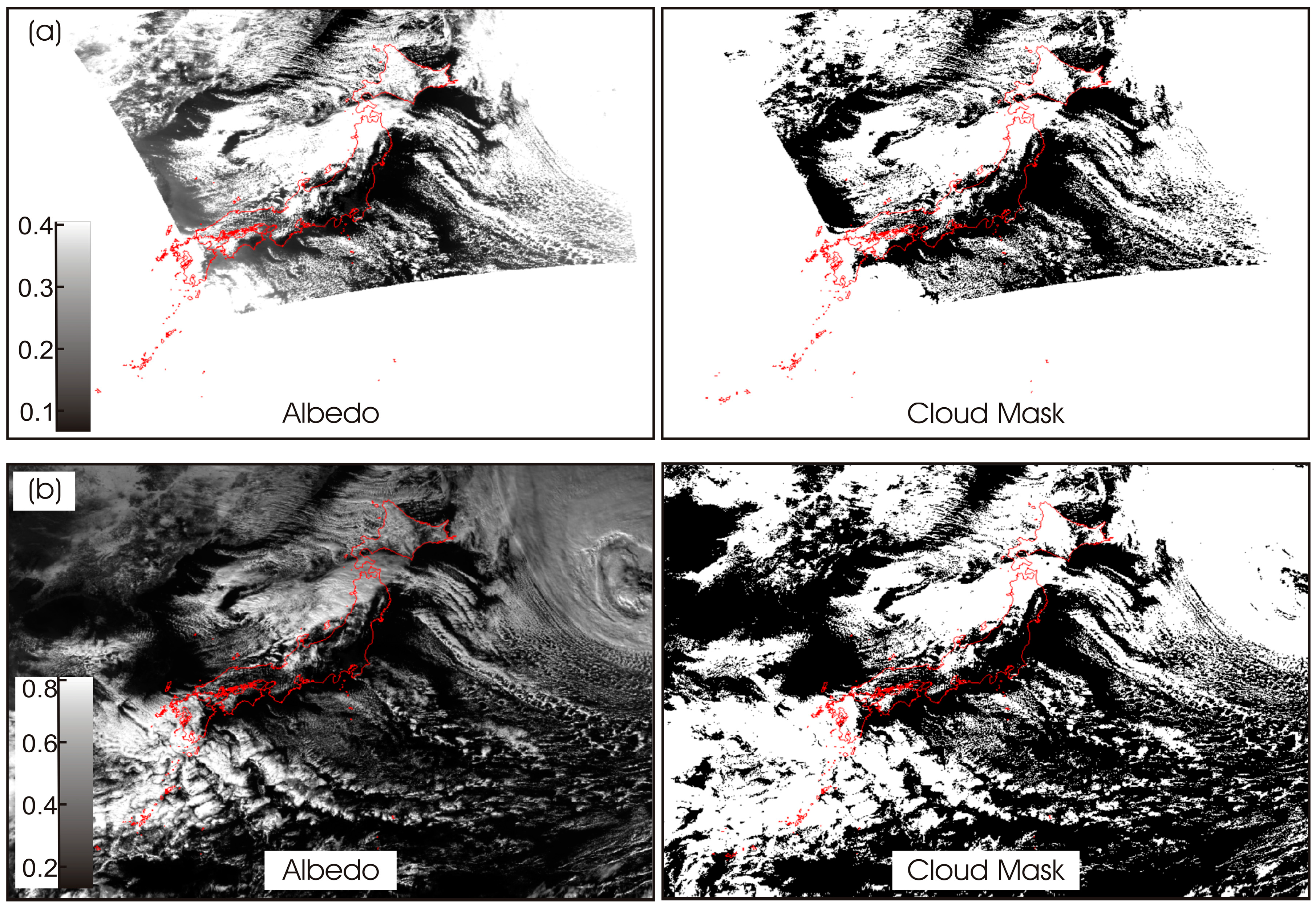
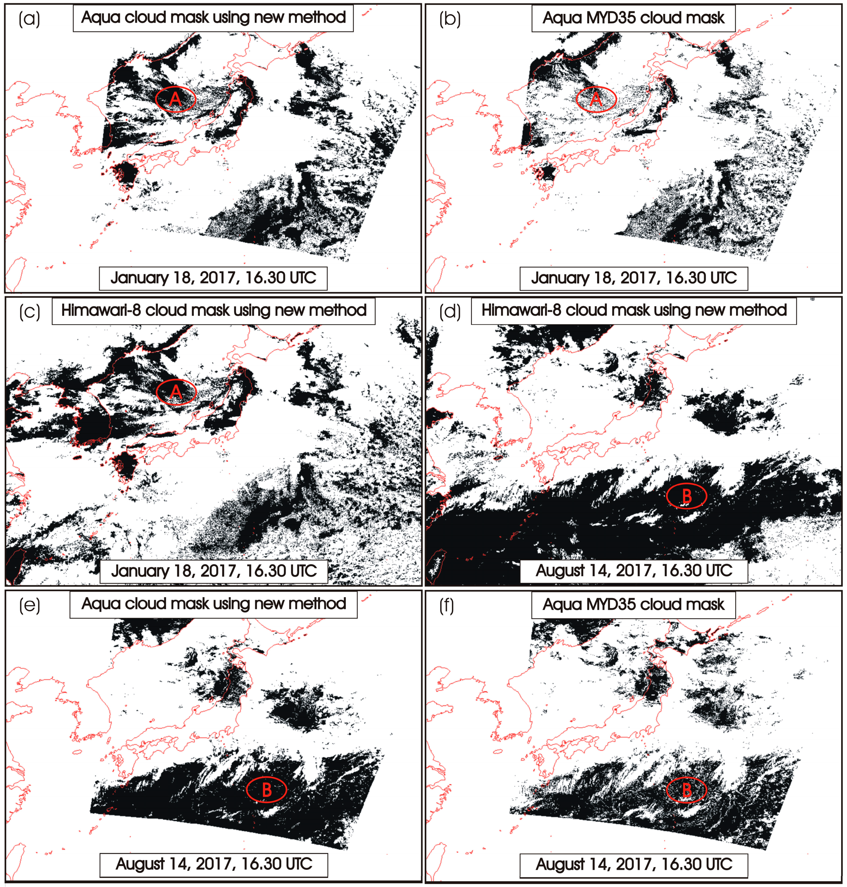
3.1. Cloud Mask
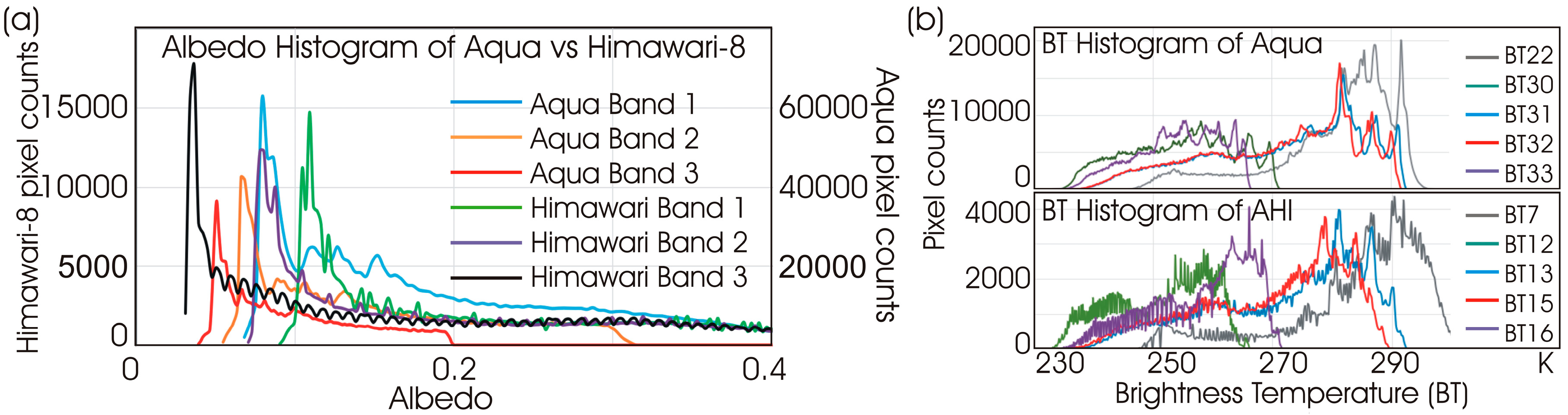
3.2. SWA Histograms
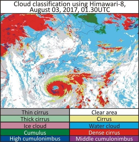
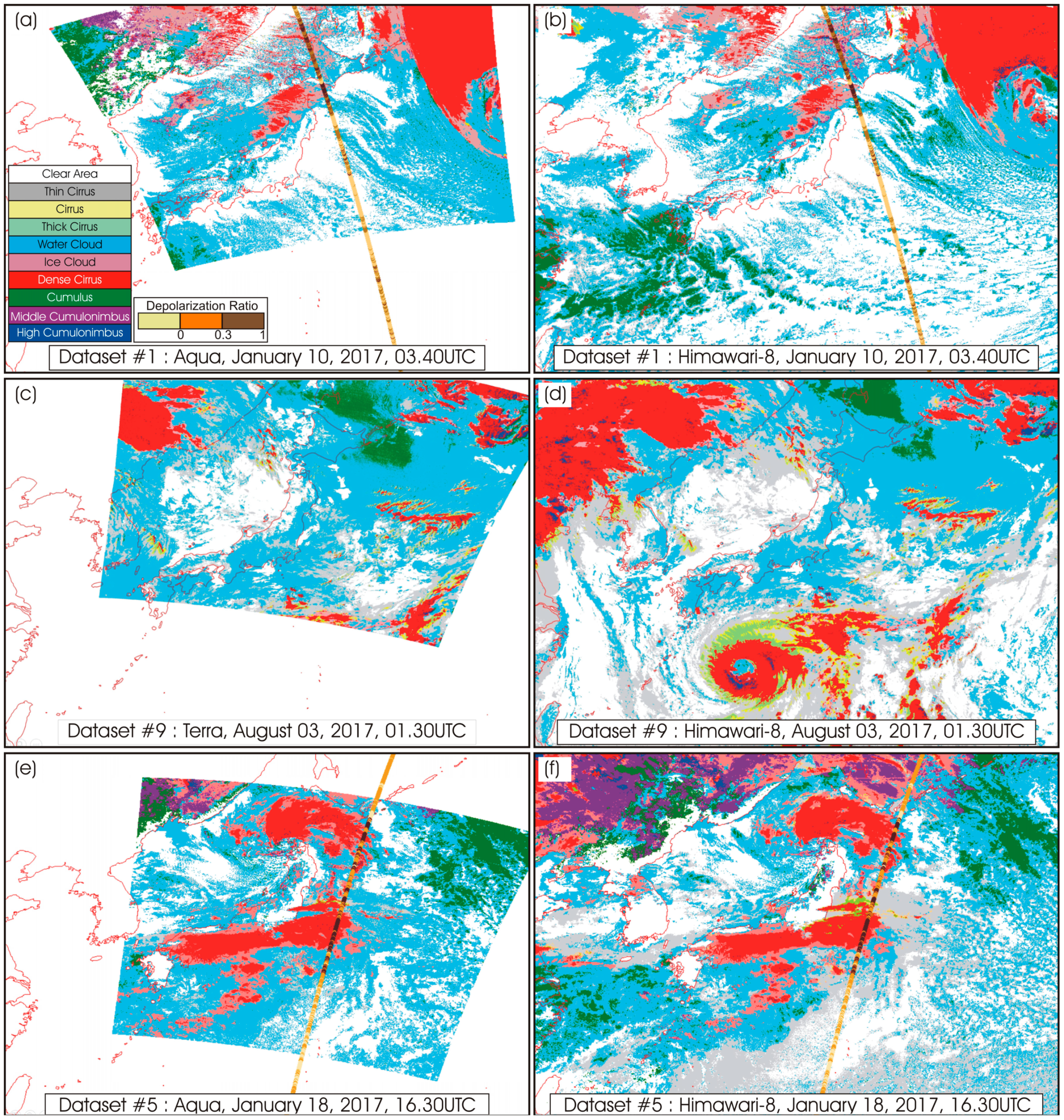
3.3. Spatial Distribution of Cloud Types
4. Discussion
4.1. Cloud Mask
4.2. POD Analysis
5. Conclusions
Author Contributions
Funding
Acknowledgments
Conflicts of Interest
References
- Schneider, S.H. Cloudiness as a Global Climatic Feedback Mechanism: The Effects on the Radiation Balance and Surface Temperature of Variations in Cloudiness. J. Atmos. Sci. 1972, 29, 1413–1422. [Google Scholar] [CrossRef] [Green Version]
- Arking, A.; Childs, J.D. Retrieval of Cloud Cover Parameters from Multispectral Satellite Images. J. Clim. Appl. Meteorol. 1985, 24, 322–333. [Google Scholar] [CrossRef] [Green Version]
- Li, J.; Menzel, W.P.; Yang, Z.; Frey, R.A.; Ackerman, S.A. High-Spatial-Resolution Surface and Cloud-Type Classification from MODIS Multispectral Band Measurements. J. Appl. Meteorol. 2003, 42, 204–226. [Google Scholar] [CrossRef]
- Li, J.; Menzel, W.P.; Sun, F.; Schmit, T.J.; Gurka, J. AIRS Subpixel Cloud Characterization Using MODIS Cloud Products. J. Appl. Meteorol. 2004, 43, 1083–1094. [Google Scholar] [CrossRef]
- Ackerman, S.A.; Strabala, K.I.; Menzel, W.P.; Frey, R.A.; Moeller, C.C.; Gumley, L.E. Discriminating Clear Sky from Clouds with MODIS. J. Geophys. Res. 1998, 103, 32141–32157. [Google Scholar] [CrossRef]
- Platnick, S.; King, M.D.; Ackerman, S.A.; Menzel, W.P.; Baum, B.A.; Riédi, J.C.; Frey, R.A. The MODIS Cloud Products: Algorithms and Examples from Terra. IEEE Trans. Geosci. Remote Sens. 2003, 41, 459–473. [Google Scholar] [CrossRef] [Green Version]
- Barnes, W.L.; Pagano, T.S.; Salomonson, V.V. Prelaunch Characteristics of the Moderate Resolution Imaging Spectroradiometer (MODIS) on EOS-AMI. IEEE Trans. Geosci. Remote Sens. 1998, 36, 1088–1100. [Google Scholar] [CrossRef] [Green Version]
- Frey, R.A.; Ackerman, S.A.; Liu, Y.; Strabala, K.I.; Zhang, H.; Key, J.R.; Wang, X. Cloud Detection with MODIS. Part I: Improvements in the MODIS Cloud Mask for Collection 5. J. Atmos. Ocean. Technol. 2008, 25, 1057–1072. [Google Scholar] [CrossRef]
- Strabala, K.I.; Ackerman, S.A.; Menzel, W.P. Cloud Properties Inferred from 8–12µm Data. J. Appl. Meteorol. Meteorol. 1994, 33, 212–229. [Google Scholar] [CrossRef] [Green Version]
- Hall, D.K.; Riggs, G.A.; Salomonson, V.V.; DiGirolamo, N.E.; Bayr, K.J. MODIS Snow-Cover Products. Remote Sens. Environ. 2002, 83, 181–194. [Google Scholar] [CrossRef] [Green Version]
- Bessho, K.; Date, K.; Hayashi, M.; Ikeda, A.; Imai, T.; Inoue, H.; Kumagai, Y.; Miyakawa, T.; Murata, H.; Ohno, T.; et al. An Introduction to Himawari-8/9. J. Meteorol. Soc. Jpn. 2016, 94, 151–183. [Google Scholar] [CrossRef] [Green Version]
- Liang, X.; Ignatov, A.; Kramar, M.; Yu, F. Preliminary Inter-Comparison between AHI, VIIRS and MODIS Clear-Sky Ocean Radiances for Accurate SST Retrievals. Remote Sens. 2016, 8, 203. [Google Scholar] [CrossRef] [Green Version]
- Qin, Y.; McVicar, T.R. Spectral Band Unification and Inter-Calibration of Himawari AHI with MODIS and VIIRS: Constructing Virtual Dual-View Remote Sensors from Geostationary and Low-Earth-Orbiting Sensors. Remote Sens. Environ. 2018, 209, 540–550. [Google Scholar] [CrossRef]
- Yuan, Y.; Hu, X. Bag-of-Words and Object-Based Classification for Cloud Extraction from Satellite Imagery. IEEE J. Sel. Top. Appl. Earth Obs. Remote Sens. 2015, 8, 4197–4205. [Google Scholar] [CrossRef]
- Christodoulou, C.I.; Michaelides, S.C.; Pattichis, C.S. Multi-feature Texture Analysis for the Classification of Clouds in Satellite Imagery. IEEE Trans. Geosci. Remote Sens. 2003, 41, 2662–2668. [Google Scholar] [CrossRef]
- Lee, Y.; Wahba, G.; Ackerman, S.A. Cloud Classification of Satellite Radiance Data by Multicategory Support Vector Machines. J. Atmos. Ocean. Technol. 2004, 21, 159–169. [Google Scholar] [CrossRef] [Green Version]
- Hay, G.J.; Castilla, G. Object-Based Image Analysis: Strengths, Weaknesses, Opportunities and Threats (SWOT). Int. Arch. Photogramm. Remote Sens. Spat. Inf. Sci. 2006, 36, 4. [Google Scholar]
- Liu, Y.; Xia, J.; Shi, C.X.; Hong, Y. An Improved Cloud Classification Algorithm for China’s FY-2C Multi-Channel Images Using Artificial Neural Network. Sensors 2009, 9, 5558–5579. [Google Scholar] [CrossRef] [Green Version]
- Inoue, T. A Cloud Type Classification with NOAA 7 Split-Window Measurements. J. Geophys. Res. 1987, 92, 3991–4000. [Google Scholar] [CrossRef]
- Inoue, T.; Ackerman, S.A. Radiative Effects of Various Cloud Types as Classified by the Split Window Technique over the Eastern Sub-tropical Pacific Derived from Collocated ERBE and AVHRR Data. J. Meteorol. Soc. Jpn. 2002, 80, 1383–1394. [Google Scholar] [CrossRef] [Green Version]
- Luo, Z.; Rossow, W.B.; Inoue, T.; Stubenrauch, C.J. Did the Eruption of the Mt. Pinatubo Volcano Affect Cirrus Properties? J. Clim. 2002, 15, 2806–2820. [Google Scholar] [CrossRef] [Green Version]
- Lutz, H.-J.; Inoue, T.; Schmetz, J. Notes and Correspondence Comparison of a Split-window and a Multi-spectral Cloud Classification for MODIS Observations. J. Meteorol. Soc. Jpn. 2003, 81, 623–631. [Google Scholar] [CrossRef] [Green Version]
- Hamada, A.; Nishi, N.; Kida, H.; Shiotani, M.; Iwasaki, S.; Kamei, A.; Ohno, Y.; Kuroiwa, H.; Kumagai, H.; Okmoto, H. Cloud type classification by GMS-5 infrared split window measurements with millimeter-wave radar and TRMM observations in the tropics. In Proceedings of the 2nd TRMM International Science Conference, Nara, Japan, 6–10 September 2004. [Google Scholar]
- Purbantoro, B.; Aminuddin, J.; Manago, N.; Toyoshima, K.; Lagrosas, N.; Sumantyo, J.T.S.; Kuze, H. Comparison of Cloud Type Classification with Split Window Algorithm Based on Different Infrared Band Combinations of Himawari-8 Satellite. Adv. Remote Sens. 2018, 7, 218–234. [Google Scholar] [CrossRef] [Green Version]
- Imai, T.; Yoshida, R. Algorithm Theoretical Basis for Himawari-8 Cloud Mask Product. Meteorol. Satell. Cent. Tech. Note 2016, 61, 1–17. Available online: https://www.data.jma.go.jp/mscweb/technotes/msctechrep61-1.pdf (accessed on 20 July 2019).
- Yamamoto, Y.; Ishikawa, H.; Oku, Y.; Hu, Z. An Algorithm for Land Surface Temperature Retrieval Using Three Thermal Infrared Bands of Himawari-8. J. Meteorol. Soc. Jpn. Ser. II 2018, 96, 43. [Google Scholar] [CrossRef] [Green Version]
- Kopp, T.J.; Thomas, W.; Heidinger, A.K.; Botambekov, D.; Frey, R.A.; Hutchison, K.D.; Iisager, B.D.; Brueske, K.; Reed, B. The VIIRS Cloud Mask: Progress in the First Year of S-NPP Toward a Common Cloud Detection Scheme. J. Geophys. Res. Atmos. 2014, 119, 2441–2456. [Google Scholar] [CrossRef]
- Murino, L.; Amato, U.; Carfora, M.F.; Antoniadis, A.; Huang, B.; Menzel, W.P.; Serio, C. Cloud Detection of MODIS Multispectral Images. J. Atmos. Ocean. Technol. 2014, 31, 347–365. [Google Scholar] [CrossRef]
- Lai, R.; Teng, S.; Yi, B.; Letu, H.; Min, M.; Tang, S.; Liu, C. Comparison of Cloud Properties from Himawari-8 and FengYun-4A Geostationary Satellite Radiometers with MODIS Cloud Retrievals. Remote Sens. 2019, 11, 1703. [Google Scholar] [CrossRef] [Green Version]
- Shang, H.; Chen, L.; Letu, H.; Zhao, M.; Li, S.; Bao, S. Development of A Daytime Cloud and Haze Detection Algorithm for Himawari-8 Satellite Measurements Over Central and Eastern China. J. Geophys. Res. 2017, 122, 3528–3543. [Google Scholar] [CrossRef]
- Ackerman, S.A.; Holz, R.E.; Frey, R.; Eloranta, E.W.; Maddux, B.C.; McGill, M. Cloud Detection with MODIS. Part II: Validation. J. Atmos. Ocean. Technol. 2008, 25, 1073–1086. [Google Scholar] [CrossRef] [Green Version]
- Derrien, M.; Farki, B.; Harang, L.; LeGléau, H.; Noyalet, A.; Pochic, D.; Sairouni, A. Automatic Cloud Detection Applied to NOAA-11/AVHRR Imagery. Remote Sens. Environ. 1993, 46, 246–267. [Google Scholar] [CrossRef]
- Trepte, Q.; Minnis, P.; Arduini, R.F. Daytime and Nighttime Polar Cloud and Snow Identification Using MODIS Data. Opt. Remote Sens. Atmos. Clouds III 2003, 4891, 449–459. [Google Scholar]
- Liu, Y.; Key, J.R.; Frey, R.A.; Ackerman, S.A.; Menzel, W.P. Nighttime Polar Cloud Detection with MODIS. Remote Sens. Environ. 2004, 92, 181–194. [Google Scholar] [CrossRef]
- Winker, D.M.; Pelon, J.R.; McCormick, M.P. The CALIPSO Mission: Spaceborne Lidar for Observation of Aerosols and Clouds. Lidar Remote Sens. Ind. Environ. Monit. III 2003, 4893, 1–11. [Google Scholar]
- Hu, Y.; Winker, D.; Vaughan, M.; Lin, B.; Omar, A.; Trepte, C.; Flittner, D.; Yang, P.; Nasiri, S.L.; Baum, B.; et al. CALIPSO/CALIOP Cloud Phase Discrimination Algorithm. J. Atmos. Ocean. Technol. 2009, 26, 2293–2309. [Google Scholar] [CrossRef] [Green Version]
- Isaacman, A.T.; Toller, G.N.; Barnes, W.L.; Guenther, B.W.; Xiong, X. MODIS Level 1B Calibration and Data Products. In Proceedings of the Optical Science and Technology, SPIE’s 48th Annual Meeting, San Diego, CA, USA, 3–8 August 2003; Volume 5151, pp. 552–562. [Google Scholar]
- Toller, G.N.; Isaacman, A.; Leader, M.T.; Salomonson, V. MODIS Level 1B Product User’s Guide. Signature 2003. Available online: https://mcst.gsfc.nasa.gov/sites/default/files/file_attachments/M1054E_PUG_2017_0901 V6.2.2_Terra_V6.2.1_Aqua.pdf (accessed on 20 July 2019).
- Japan Meteorological Agency Himawari-8/9 Standard Data User’s Guide Version 1.2. 2015. Available online: https://www.data.jma.go.jp/mscweb/en/himawari89/space_segment/hsd_sample/HS_D_users_guide_en_v12.pdf (accessed on 20 July 2019).
- Wylie, D.P.; Menzel, W.P. Eight Years of High Cloud Statistics Using HIRS. J. Clim. 1999, 12, 170–184. [Google Scholar] [CrossRef]
- Cho, H.-M.; Yang, P.; Kattawar, G.W.; Nasiri, S.L.; Hu, Y.; Minnis, P.; Trepte, C.; Winker, D. Depolarization Ratio and Attenuated Backscatter for Nine Cloud Types: Analyses Based on Collocated CALIPSO Lidar and MODIS Measurements. J. Geophys. Res. Atmos. 2008, 16, 3931–3948. [Google Scholar] [CrossRef]
- Hu, Y. Depolarization Ratio–Effective Lidar Ratio Relation: Theoretical Basis for Space Lidar Cloud Phase Discrimination. Geophys. Res. Lett. 2007, 34, 6–9. [Google Scholar] [CrossRef]
- Hu, Y.X.; Yang, P.; Lin, B.; Gibson, G.; Hostetler, C. Discriminating Between Spherical and Non-Spherical Scatterers with Lidar Using Circular Polarization: A Theoretical Study. J. Quant. Spectrosc. Radiat. Transf. 2003, 79, 757–764. [Google Scholar] [CrossRef]
- Hu, C. An Empirical Approach to Derive MODIS Ocean Color Patterns under Severe Sun Glint. Geophys. Res. Lett. 2011, 38, 1–5. [Google Scholar] [CrossRef]
- Wang, M.; Bailey, S.W. Correction of Sun Glint Contamination on the Sea WiFS Ocean and Atmosphere Products. Appl. Opt. 2001, 40, 4790–4798. [Google Scholar] [CrossRef] [PubMed]
- Lee, S.H.; Kim, B.Y.; Lee, K.T.; Zo, I.S.; Jung, H.S.; Rim, S.H. Retrieval of Reflected Shortwave Radiation at the Top of the Atmosphere Using Himawari-8/AHI Data. Remote Sens. 2018, 10, 213. [Google Scholar] [CrossRef] [Green Version]
- Zhang, H.; Wang, M. Evaluation of Sun Glint Models Using MODIS Measurements. J. Quant. Spectrosc. Radiat. Transf. 2010, 111, 492–506. [Google Scholar] [CrossRef]
- Frei, A.; Tedesco, M.; Lee, S.; Foster, J.; Hall, D.K.; Kelly, R.; Robinson, D.A. A Review of Global Satellite-Derived Snow Products. Adv. Space Res. 2012, 50, 1007–1029. [Google Scholar] [CrossRef] [Green Version]
- Shang, H.; Letu, H.; Nakajima, T.Y.; Wang, Z.; Ma, R.; Wang, T.; Lei, Y.; Ji, D.; Li, S.; Shi, J. Diurnal Cycle and Seasonal Variation of Cloud Cover over the Tibetan Plateau as Determined from Himawari-8 New-Generation Geostationary Satellite Data. Sci. Rep. 2018, 8, 1105. [Google Scholar] [CrossRef]
- Xia, L.; Zhao, F.; Chen, L.; Zhang, R.; Mao, K.; Kylling, A.; Ma, Y. Performance Comparison of the MODIS and the VIIRS 1.38 μm Cirrus Cloud Channels Using LibRadtran and CALIOP Data. Remote Sens. Environ. 2018, 206, 363–374. [Google Scholar] [CrossRef]
- Wang, J.; Liu, C.; Min, M.; Hu, X.; Lu, Q.; Husi, L. Effects and Applications of Satellite Radiometer 2.25μm Channel on Cloud Property Retrievals. IEEE Trans. Geosci. Remote Sens. 2018, 56, 5207–5216. [Google Scholar] [CrossRef]
- Wang, J.; Liu, C.; Yao, B.; Min, M.; Letu, H.; Yin, Y.; Yung, Y.L. A Multilayer Cloud Detection Algorithm for the Suomi-NPP Visible Infrared Imager Radiometer Suite (VIIRS). Remote Sens. Environ. 2019, 227, 1–11. [Google Scholar] [CrossRef]
- Wang, T.; Fetzer, E.J.; Wong, S.; Kahn, B.H.; Yue, Q. Validation of MODIS Cloud Mask and Multilayer Flag Using CloudSat-CALIPSO Cloud Profiles and a Cross-Reference of their Cloud Classifications. J. Geophys. Res. Atmos. 2016, 121, 11620–11635. [Google Scholar] [CrossRef]


| #Dataset | Date | Aqua/Terra MODIS | Himawari-8 AHI | CALIPSO | Season (Day/Night) |
|---|---|---|---|---|---|
| 1 | 10 January 2017 | Aqua: 03.40 UTC | 03.40 UTC | 03.41–03.53 UTC | Winter (Day) |
| 2 | 11 February, 2017 | Aqua: 03.40 UTC | 03.40 UTC | 03.30–03.44 UTC | Winter (Day) |
| 3 | 23 January 2017 | Terra: 01.30 UTC | 01.30 UTC | no overpass data | Winter (Day) |
| 4 | 24 February 2017 | Terra: 01.30 UTC | 01.30 UTC | no overpass data | Winter (Day) |
| 5 | 18 January 2017 | Aqua: 16.30 UTC | 16.30 UTC | 16.29–16.42 UTC | Winter (Night) |
| 6 | 08 July 2017 | Aqua: 04.10 UTC | 04.10 UTC | 04.11–04.25 UTC | Summer (Day) |
| 7 | 06 August 2017 | Aqua: 03.40 UTC | 03.40 UTC | 03.39–03.52 UTC | Summer (Day) |
| 8 | 18 July 2017 | Terra: 01.30 UTC | 01.30 UTC | no overpass data | Summer (Day) |
| 9 | 03 August 2017 | Terra: 01.30 UTC | 01.30 UTC | no overpass data | Summer (Day) |
| 10 | 14 August 2017 | Aqua: 16.30 UTC | 16.30 UTC | 16.25–16.39 UTC | Summer (Night) |
| 1. Daytime Cloud Masking | |||
|---|---|---|---|
| Clear Area | Cloudy Area | ||
| Himawari-8 | Summer and winter | R1 < 0.2 | R1 ≥ 0.2 |
| Aqua/Terra MODIS | Summer and winter | R3 < 0.12 | R3 ≥ 0.12 |
| 2. Nighttime cloud masking | |||
| Himawari-8 AHI Winter | Land Area | BT13 ≥ 256 K and BTD13-16 ≥ 8.2 K | Otherwise |
| Sea Area | BT7 ≥ 270 K and BTD7-13 ≤ 0.3 K | Otherwise | |
| Himawari-8 AHI Summer | Land Area | BT7 ≥ 275 K and BT7-12 ≥ 23.2 K | Otherwise |
| Sea Area | BT7 ≥ 284 K and BTD7-13 ≤ 4.4 K | Otherwise | |
| Aqua MODIS Winter | Land Area | BT31 ≥ 258 K and BTD31-33 ≥ 11.5 K | Otherwise |
| Sea Area | BT22 ≥ 271 K and BTD22-31 ≤ 1.5 K | Otherwise | |
| Aqua MODIS Summer | Land Area | BT22 ≥ 286 K and BTD22-30 ≥ 5.8 K | Otherwise |
| Sea Area | BT22 ≥ 271 K and BTD22-31 ≤ 1.5 K | Otherwise | |
| AHI (Himawari-8) | MODIS (Aqua/Terra) | |||||
|---|---|---|---|---|---|---|
| #Band | Central Wavelength (m) | Pixel Size (km) | #Band | Central Wavelength (m) | Pixel Size (km) | |
| Visible | 1 | 0.47 | 1 | 3 | 0.469 | 0.5 |
| Infrared | 7 | 3.9 | 2 | 22 | 3.96 | 1 |
| 12 | 9.6 | 2 | 30 | 9.73 | 1 | |
| 13 | 10.4 | 2 | − | − | − | |
| 14 | 11.2 | 2 | 31 | 11.03 | 1 | |
| 15 | 12.4 | 2 | 32 | 12.02 | 1 | |
| 16 | 13.3 | 2 | 33 | 13.335 | 1 | |
| Aqua (SWA31-32) | Terra (SWA31-32) | Himawari-8 (SWA13-15) | ||||
|---|---|---|---|---|---|---|
| Season | winter | summer | winter | summer | winter | summer |
| BT-1 | 245 | 249 | 242 | 246 | 245 | 250 |
| BT-2 | 254 | 257 | 250 | 253 | 253 | 258 |
| BTD-1 | 0.0 | 0.0 | 0.0 | 0.0 | 0.6 | 0.9 |
| BTD-2 | 2.1 | 1.7 | 2.1 | 1.7 | 3.2 | 4.5 |
| #Dataset | Date | Time (UTC) | Cloud Mask | Cloud Classification | ||
|---|---|---|---|---|---|---|
| POD MODIS | POD AHI | POD MODIS | POD AHI | |||
| 1 | 10 January 2017 | 03.40 | 83.8% | 79.0% | 74.0% | 77.2% |
| 2 | 11 February 2017 | 03.40 | 87.3% | 83.4% | 68.5% | 74.5% |
| 3 | 23 January 2017 | 01.30 | 88.4% | 85.3% | − | − |
| 4 | 24 February 2017 | 01.30 | 88.1% | 83.6% | − | − |
| 5 | 18 January 2017 | 16.30 | 86.1% | 82.1% | 71.9% | 69.0% |
| 6 | 08 July 2017 | 04.10 | 70.2% | 89.5% | 60.3% | 60.2% |
| 7 | 06 August 2017 | 03.40 | 83.6% | 85.5% | 73.2% | 62.6% |
| 8 | 18 July 2017 | 01.30 | 86.7% | 81.9% | − | − |
| 9 | 03 August 2017 | 01.30 | 78.6% | 81.8% | − | − |
| 10 | 14 August 2017 | 16.30 | 88.4% | 86.2% | 72.2 | 75.4 |
© 2019 by the authors. Licensee MDPI, Basel, Switzerland. This article is an open access article distributed under the terms and conditions of the Creative Commons Attribution (CC BY) license (http://creativecommons.org/licenses/by/4.0/).
Share and Cite
Purbantoro, B.; Aminuddin, J.; Manago, N.; Toyoshima, K.; Lagrosas, N.; Sumantyo, J.T.S.; Kuze, H. Comparison of Aqua/Terra MODIS and Himawari-8 Satellite Data on Cloud Mask and Cloud Type Classification Using Split Window Algorithm. Remote Sens. 2019, 11, 2944. https://doi.org/10.3390/rs11242944
Purbantoro B, Aminuddin J, Manago N, Toyoshima K, Lagrosas N, Sumantyo JTS, Kuze H. Comparison of Aqua/Terra MODIS and Himawari-8 Satellite Data on Cloud Mask and Cloud Type Classification Using Split Window Algorithm. Remote Sensing. 2019; 11(24):2944. https://doi.org/10.3390/rs11242944
Chicago/Turabian StylePurbantoro, Babag, Jamrud Aminuddin, Naohiro Manago, Koichi Toyoshima, Nofel Lagrosas, Josaphat Tetuko Sri Sumantyo, and Hiroaki Kuze. 2019. "Comparison of Aqua/Terra MODIS and Himawari-8 Satellite Data on Cloud Mask and Cloud Type Classification Using Split Window Algorithm" Remote Sensing 11, no. 24: 2944. https://doi.org/10.3390/rs11242944