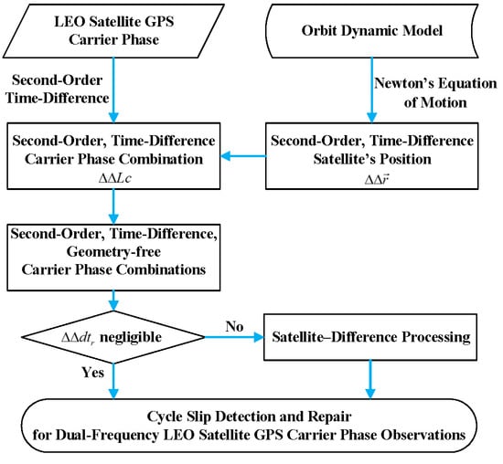
Cycle Slip Detection and Repair for Dual-Frequency LEO Satellite GPS Carrier Phase Observations with Orbit Dynamic Model Information


School of Geodesy and Geomatics, Wuhan University, Wuhan 430070, China
*
Author to whom correspondence should be addressed.
Remote Sens. 2019, 11(11), 1273; https://doi.org/10.3390/rs11111273
Submission received: 19 April 2019
/
Revised: 24 May 2019
/
Accepted: 27 May 2019
/
Published: 29 May 2019
(This article belongs to the Special Issue High-precision GNSS: Methods, Open Problems and Geoscience Applications)
Abstract
:Cycle slip detection and repair are crucial for precise GPS-derived orbit determination of the low-Earth orbit (LEO) satellites. We present a new approach to detect and repair cycle slips for dual-frequency LEO satellite GPS observations. According to Newton’s equation of motion, the second-order time difference of the LEO satellite’s position (STP) is only related to the sampling interval and the satellite’s acceleration, which can be precisely obtained from the known orbit dynamic models. Then, several kinds of second-order time-difference geometry-free (STG) phase combinations, taking full advantage of the correlation between the satellite orbit variations and the dynamic model, with different level of ionospheric residuals, are proposed and adopted together to detect and fix cycle slips. The STG approach is tested with some LEO satellite GPS datasets. Results show that it is an effective cycle slip detection and repair method for LEO satellite GPS observations. This method also has some important features. Firstly, the STG combination is almost independent of the pseudorange. Secondly, this method is effective for LEO satellites, even in real-time application. Thirdly, this method is suitable for ground-based GPS receivers if we know the acceleration of the receivers.
1. Introduction
As GPS carrier phase observations are much more accurate than pseudorange observations, carrier phase measurements are usually used as observations for the precise GPS-derived orbit determination of low-Earth orbit (LEO) satellites [1,2,3,4,5]. Compared to ground GPS data, due to the high-speed motion and complicated observation environment of LEO satellites, cycle slips occur frequently in LEO satellite GPS carrier phase data, which are undesirable and must be detected and repaired correctly to maintain the continuity of GPS carrier phase observations.
The difficulties of cycle slip detection are as follows: (i) the geometric distance between receiver and satellite varies greatly; (ii) the ionospheric delay varies quickly. How to eliminate the influence of geometric distance and ionospheric delay, and construct an effective quantity that is sensitive to the cycle slips is the key point of cycle slip detection. In the past, a variety of cycle slip detection methods for dual-frequency GPS signals were proposed. According to the strategy to eliminate the geometric distance, these methods can be divided into two categories, described below.
The first category encompasses linear combination methods, where the linear combinations of observations at different frequencies are formed to eliminate the geometric distance, including the Hatch–Melbourne–Wübbena (HMW) combination [6,7,8] and the geometry-free phase combination [9]. The HMW combination is widely used to detect cycle slips for dual-frequency GPS data of both static and kinematic receivers. However, this method is not suitable for data with the same size of cycle slips on both L1 and L2 frequencies. In order to detect all potential cycle slips, a complementary method must be adopted, such as the traditional TurboEdit method [10]. However, TurboEdit may fail to detect small cycle slips of 1–2 cycles due to the large pseudorange noise [11]. The geometry-free phase combination is also usually used to detect cycle slips along with the HMW combination. This combination, however, contains ionospheric residuals and has a wavelength of only 5.4 cm for cycle slips, which is only effective for the cases when the ionosphere is stable. Some modifications of the phase combination with different techniques were also proposed, such as polynomial fitting [12,13], Kalman filter [14,15,16], higher-order time difference [17,18], cycle slip detection by integrating an inertial navigation system and GPS [19,20], double- or triple-epoch difference residuals [21], and Bayesian theory [22]. In addition, Liu [23] applied the ionospheric total electron content rate (TECR) to detect cycle slips. Cai et al. [11] proposed a method based on a forward- and backward-moving window averaging algorithm integrated with a second-order time-difference phase ionospheric residual (STPIR) algorithm. As the backward-moving technique is used, it is utilized for post-processing. Having smooth phase observations is an underlying assumption of many of these cycle slip detection methods. This assumption can be violated under high ionospheric activities [24].
The second category encompasses estimation methods, where the first-order or second-order time-difference observations of carrier phase and pseudorange observations are formed; then, the position variations are estimated along with the receiver clock variation, the ionospheric delay variations, and the cycle slips [25,26]. Due to the numerous unknown parameters, the introduction of reasonable constraints of the ionospheric delay variations is necessary. Incorrect cycle slip determination may be caused when there are irregular rapid ionospheric variations. Li et al. [27] developed a geometry-based ionosphere-weighted (GBIW) model dedicated to efficiently estimating cycle slips in scenarios with active ionospheric conditions. However, consecutive historical data are necessary for the prediction of between-epoch ionospheric variations under high ionospheric activities or in the case of a large sampling interval/data gap.
As for the satellite-borne GPS receiver, the ionospheric residuals in carrier phase observations clearly vary and cannot be removed by differences in measurements in adjacent epochs, and consecutive historical ionospheric residual data are hardly available, which makes many of the methods related to the ionosphere ineffective. Bae et al. [28] and Montenbruck et al. [1,29] used a priori orbit as a reference to detect cycle slips with ionosphere-free linear combinations. However, because carrier phase measurements are essential for precise GPS orbit determination, it is an iteration process that detects cycle slips, and the detection effect is affected by the accuracy of the a priori orbit.
In this research, we present a second-order, time-difference, geometry-free (STG) approach to detect and repair cycle slips for LEO satellite GPS carrier phase observations with orbit dynamic model information. According to a reformulation of Newton’s equation of motion, the second-order time difference of the LEO satellite’s position (STP) is only related to the satellite’s acceleration and the sampling interval, regardless of velocity. Therefore, the STP value can be computed, with an accuracy that is only affected by the accuracy of the a priori acceleration. Moreover, the precise dynamic orbit determination of the GPS/LEO satellite [3,5,30,31] shows that it is possible to obtain a high-precision acceleration estimate of satellites with the known orbit dynamic models. By substituting the STP values into the carrier phase observations, the STG observations are derived. In this paper, unlike the traditional HMW combination and the geometry-free phase combination, four STG combinations with different levels of ionospheric residuals are adopted together to detect and repair cycle slips.
The remainder of the paper is organized as follows: In Section 2, the STG cycle slip detection and repair approach is presented. The experiments and analysis are presented in Section 3 to assess the performances of the proposed method in various cases. Finally, concluding remarks are summarized, and an outlook for future research is presented in Section 4.
2. Materials and Methods
This article is based on the analysis of GPS products, LEO precise orbit products, and LEO GPS observation datasets obtained from different sources. The second-order, time-difference carrier phase liner combination is presented. Then, based on the relationship between the STP value and the satellite’s acceleration, the STG cycle slip detection and repair approach is described in detail.
2.1. GPS and LEO Data
In order to investigate the performance of the proposed STG cycle slip detection and repair method, the analysis of our paper is based on the GPS products (provided by the International GNSS Service (IGS)), LEO precise orbit products (GOCE, GRACE-A, and Jason-3 satellites provided by the European Space Agency (ESA), Jet Propulsion Laboratory (JPL), and CNES, respectively), and GOCE satellite GPS observations provided by the ESA. Here, we tested GOCE satellite phase observations in November 2009, with a 1-Hz sampling rate.
2.2. Second-Order, Time-Difference Carrier Phase Combination
The dual-frequency (subscript 1/2 for carriers L1/L2) observations between the LEO satellite receiver (subscript ) and GPS satellites (superscript ) are commonly described as
where is the velocity of light, is the geometric distance between the GPS satellite and receiver, are the dual-frequency carrier phase observations, are the carrier phases, wavelengths, and ambiguities at frequencies , respectively, are the clock offset of the GPS satellite and receiver, respectively, , is the ionospheric delay, and are the noise of the dual-frequency carrier phase observations.
The antenna phase center correction, relativistic effect, and wind-up effect, which can be calculated with the known correction models, are eliminated in Equation (1). For simplicity of expression, the time epoch of some symbols is omitted, such as for , whereas subscript and superscript are also omitted in some of the following equations. Given Equation (1), the linear combination of carrier phase can be described as follows:
where and are coefficients of the observations and , respectively.
Assuming the true position of the GPS satellite and receiver’s mass center are and , respectively, and the approximate positions are and , respectively, then we have
where is the geometric distance between and , is unit direction vector between the GPS satellite and receiver, and .
With Equations (2) and (3), the second-order, time-difference carrier phase combination can be represented as
Let us analyze the terms in Equation (4). is available from the GPS broadcast ephemeris in the real-time application or IGS final precise ephemeris products in the post-processing applications, and is available from a LEO a priori orbit, e.g., a GPS code solution [32]. Thus, can be treated as known. Moreover, the term can be given as
since
Considering the altitude of the GPS satellite, is usually larger than 20,000 km, even for LEO satellites. Additionally, the GPS and LEO satellite velocities are approximately 4 km/s and 8 km/s, respectively. Then, we have
Thus, the maximum amplitude of is less than 2 × 10⁻², even with 30-s sampling intervals. Therefore, the last two terms and in Equation (5) can be ignored.
The STP values and can be derived with the satellite orbit dynamic models (presented in Section 2.3. Thus, in Equation (4) can be treated as known and used to remove the geometric variations between the receiver and the GPS satellites. The second-order, time-difference GPS clock errors are very small, due to the high-stability atomic clocks equipped on the GPS satellites, which can be practically ignored for cycle slip detection and repair (presented in Section 3).
Moreover, for LEO satellite GPS data, STPIR is significantly smaller than the first-order, time-difference phase ionospheric residual (PIR), which is similar to the ground-based GPS data [11]. What is more, as the distance variations are removed, several kinds of STG combinations can be formed to reduce the ionospheric residuals further, as shown in the next section. The numerical results and analysis of the second-order time-difference values mentioned above, , , , and , are presented in Section 3.
2.3. Second-Order Time Difference of the Satellite’s Position
Based on a reformulation of Newton’s equation of motion, the second-order time difference of the satellite’s position can be given as by Ditmar and van der Sluijs [33].
where
is the second-order time-difference (ST) operator, in which and refer to three consecutive epochs, and and are the satellite’s position and acceleration at time epoch .
Equation (8) is considered as the basic constraint in our work, which shows that the STP value is only related to the acceleration and sampling interval . Since , the accuracy requirements of acceleration for different sampling intervals with an error at the 1-cm level can be given as , as shown in Table 1. Thus, the errors or magnitudes of the accelerations less than the requirements can be practically ignored. In fact, most of the accelerations of LEOs are below 10−4 ms−2 [34].
The precise dynamic orbit determination of the GPS and LEO satellites shows that it is usually possible to obtain the satellites’ acceleration from known orbit dynamic models, with an accuracy better than 10−5 ms−2 [3,4,30,31]. Therefore, the STP values and can be computed via Equation (8), and used to remove the geometric variations in GPS data without a high-precision a priori orbit.
What is more, in the real-time application, given a priori orbit error (broadcast ephemeris for GPS satellites [35], a real-time GPS code solution for LEO satellites), the max acceleration error comes from the Earth’s center of gravity.
where is the Earth’s gravitational constant, is the distance from the satellite to the Earth’s center, and .
As Table 1 suggests, can be practically ignored, even for 30-s intervals. Thus, the term in Equation (4) can be derived precisely, even in real-time applications.
2.4. STG Cycle Slip Detection Method
We can make a satellite–difference combination to remove the second-order, time-difference receiver clock errors . Thus, with Equation (4), the STG cycle slip detection values can be given as
where is the satellite–difference operator, and represent the different GPS satellites, and .
As stated above, the first part of the right side of Equation (9) can be precisely computed from the GPS phase observations and the known orbit dynamic models. Based on Equation (9), we can have several STG combinations, with different levels of ionospheric residuals as follows:
The coefficients and are shown in Table 2, corresponding to Equations (10)–(13).
Equations (10)–(13) can be used to detect cycle slips, as Equation (10) is ionospheric-free, and Equations (11) and (12) have smaller ionospheric residuals ( and ) to STPIR (). Furthermore, Equation (13) can be used for big cycle slip detection for single-frequency GPS carrier phase data, where even cannot be practically ignored.
If cycle slips occur on GPS L1 and L2 frequencies between time epochs and , due to the second-order time-difference processing, by adding the time epoch mark with Equation (9), we have the cycle slip values as follows:
Equations (14) and (15) suggest that there will be two opposite peak values in the subsequent epochs when cycle slips occur, which can be used together to detect cycle slips.
Moreover, it should be pointed out that for some LEO satellites (e.g., GOCE) can also be practically ignored, due to the high-stability atomic clocks usually equipped, similar to the GPS satellites. In that case, the satellite–difference operator is not necessary for Equations (9)–(15) (presented in Section 3).
2.5. Repair of Cycle Slips Using the STG Combinations
Any combination of Equations (10)–(13) alone can be used to detect cycle slips except for some special cycle slip pairs (CSPs) . For instance, when the CSPs are , the detected cycle slip value in Equation (10) is 0, because these CSPs do not result in a change in . Similarly, special CSPs, such as , do not show jumps in the combination of Equation (11), and Equation (12) cannot detect CSPs such as .
Fortunately, the joint STG combinations can complement individual drawbacks. For instance, for the CSP (1, 1), Equation (11) is insensitive, but Equation (10) has a value of 0.22 cycles, and Equation (12) has a value of 0.3583 cycles, while Equation (13) has a value of one cycle, which can be detected easily. Rows 3–6 in Table 3 refer to some special CSPs that are insensitive for some of STG combinations.
What is more, although Equation (13) seems to be suitable for estimating cycle slips for single-frequency GPS observations alone, the ionospheric residual in Equation (13) is larger than the other combinations. Thus, it is suggested to adopt all the combinations in Equations (10)–(13) together to detect and repair cycle slips for dual-frequency LEO satellite GPS observations.
When cycle slips are detected using combinations from Equations (10)–(13), the values of cycle slips can be uniquely determined from the following equations:
where are the detected cycle slip values, corresponding to Equations (10)–(13), respectively. Based on Equation (16), the float cycle slip solutions are firstly solved and then the integer solutions are determined, e.g., using the LAMBDA method proposed by Teunissen [36].
3. Results and Discussion
This section presents the results and analysis of the second-order time-difference values related to the STG cycle slip detection and repair method, and investigates the performance of the proposed method using the GPS observations of the GOCE satellite.
3.1. Analysis of the Second-Order Time-Difference Values for LEO GPS Observations
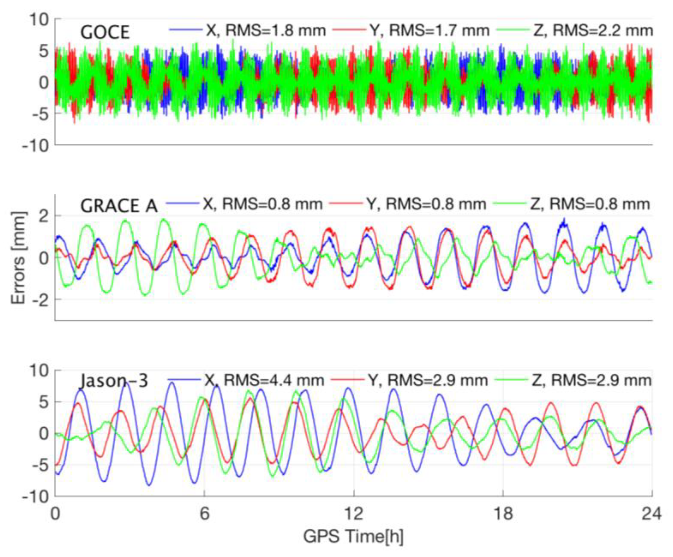
Firstly, we evaluate the errors of the computed and via Equation (8), with the known orbit dynamic models, with different sampling intervals, with the final precise ephemeris products for GPS satellites and LEO satellites (GOCE, GRACE-A, and Jason-3 satellite) as “true” values. Based on one-day data, the errors of the computed and are shown in Figure 1 and Figure 2. Here, only the Earth gravity model 2008 (EGM2008) up to 120 degrees and order is used as the known dynamic model to compute the and for the satellites, with for GOCE and GRACE, and for Jason-3 (corresponding to Jason-3′s orbit product). The results show that the computed errors all are less than 3 mm for all GPS satellites in three directions, while the RMSs of the computed error in the three directions are 1.8 mm, 1.7 mm, and 2.2 mm for GOCE, 0.8 mm, 0.8 mm, and 0.8 mm for GRACE-A, and 4.4.mm, 2.9 mm, and 2.9 mm for Jason-3.
On one hand, due to GOCE’s lower orbital altitude (about 260 km), the ignored gravitational accelerations (e.g., ocean tide, solid tide) are stronger than for GRACE. Thus, the errors of the computed STPs of GOCE are larger than those of GRACE. On the other hand, the errors of the computed STPs of Jason-3 are larger than those of GOCE and GRACE, because of the larger sample interval. The results are consistent with Equation (8). Moreover, the STP accuracies are still better than 0.01 m. Therefore, it can be concluded that the errors of the computed STPs and computed via Equation (8) are negligible for cycle slip detection and repair.
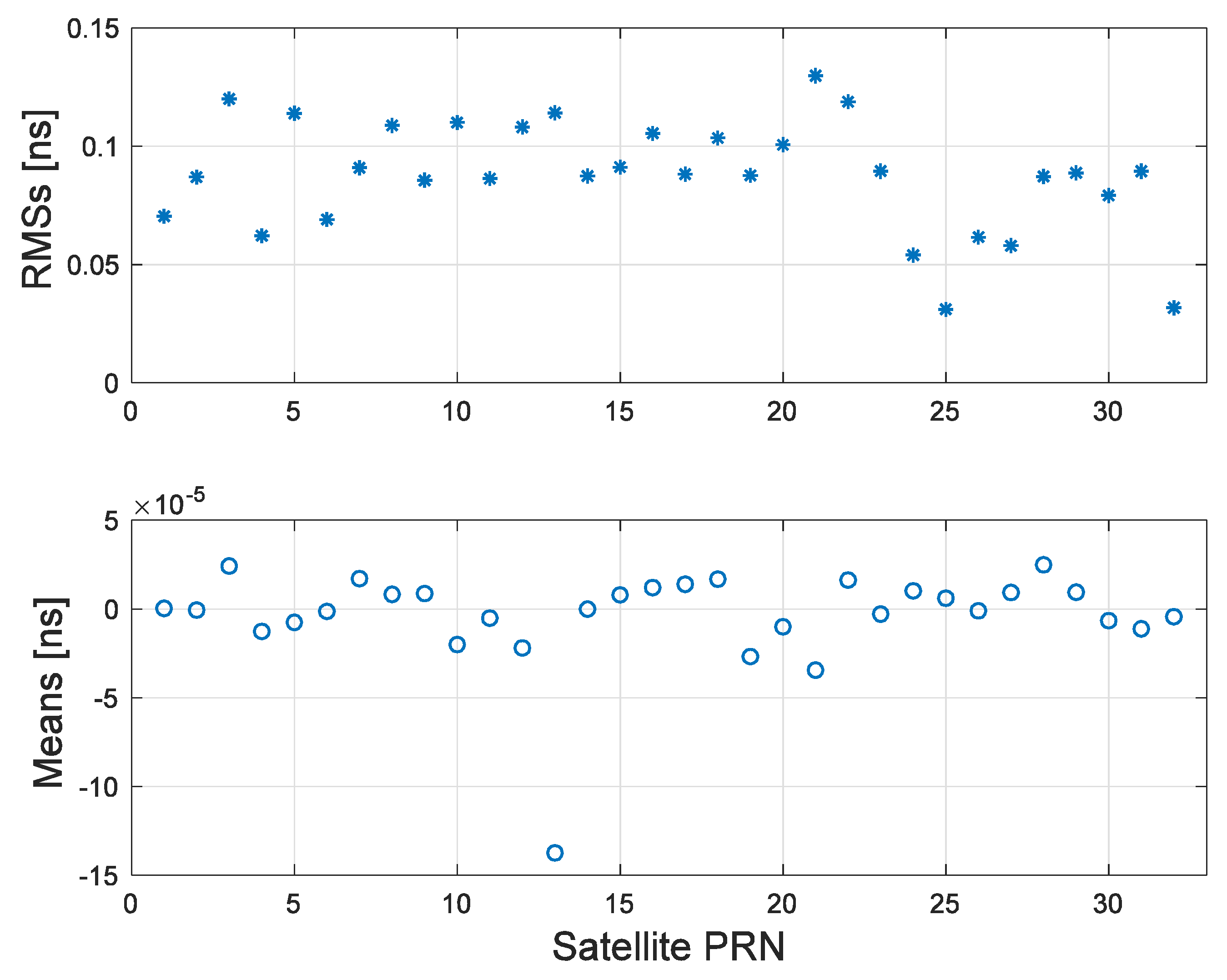
Furthermore, with one-day (18 November 2009) final 30-s clock products provided by IGS as the “true” values, is evaluated, and the means and RMSs of are statistically computed for a sampling interval of 30 s, as shown in Figure 3. The results clearly illustrate that values are as precise as 0.1 ns with nearly zero means for most GPS satellites, and are all smaller than 0.15 ns, which means that can also be practically ignored for cycle slip detection and repair.
Finally, as the ionosphere residuals in carrier phase observations vary quickly for LEO satellite GPS data, one may have the question whether can be practically ignored in the estimation of cycle slips for satellite-borne GPS observations, even with a 1-s sampling interval. To answer this question, Figure 4 and Figure 5 show the examples of the first-order, time-difference PIR and STPIR [11] () at the GOCE satellite on 26 November 2009, with different sampling intervals. As shown in Figure 4 and Figure 5, firstly, STPIR values increase and vary more quickly as the sampling interval grows, especially at low elevation angles and near polar areas, where the quality of the carrier phase observations is poor [3,28]. Secondly, STPIR values are usually less than 0.02 m (about 0.1 cycles) with 1-s sampling intervals, always less than 0.05 m (about 0.25 cycles) with 5-s sampling intervals, and less than 0.1 m (about 0.5 cycles) with 10-s sampling intervals. Moreover, STPIR is significantly smaller than the first-order, time-difference PIR for GOCE. It suggests that STPIR (0.6469 ) is negligible for cycle slip detection for LEO satellite phase observations, especially with a 1-Hz sampling rate, based on the conditions tested.
Therefore, the second-order time-difference values for LEO GPS observations given in Equation (9), , , , and , can be practically used as known or ignored for the proposed STG cycle slip detection and repair method.
3.2. Using the Proposed STG Method to Detect and Repair Cycle Slips
In order to investigate the performance of the proposed STG cycle slip detection and repair method, the GPS observation data of GOCE satellite on 21 November 2009 were collected with a sampling interval of 1 s. Figure 6 shows GOCE satellite latitude, elevation, and STPIR (1 s) for GPS PRN 9 and PRN 22 (max elevation 2.1°). Due to the lower elevation, the quality of the carrier phase observations corresponding to PRN 22 is poor. Firstly, simulated special CSPs were added to the GPS L1 and L2 carrier phase data every 5 min, from 5:20 to 5:45 p.m. (GPS time) for PRN 9, and from 5:35 to 5:45 p.m. (GPS time) for PRN 22, as shown in Table 4.
Figure 7 and Figure 8 show the cycle slip detection results for the testing data with special CSPs using the STG method, without the satellite–difference processing. For convenience of display, the detected cycle slip values larger than 1.5 cycles were set as 1.5 in the figures below. In each plot, time series of the combinations from Equations (10)–(13) are shown. The time series of the ionosphere-free STG combination in Equation (10) shown in Figure 7 and Figure 8 are stable at zero cycles, which indicates that the geometric variations are removed clearly, and GOCE’s can be practically ignored, similar to the GPS satellites, due to the high-stability atomic clocks equipped [3]. The STG combinations in Equations (11)–(13) are also stable at zero cycles, which illustrates that the ionospheric residuals for GOCE are significantly small and negligible in our work. Moreover, as Equations (14) and (15) suggested, there are two opposite peak values in the adjacent epochs when the cycle slip is simulated.
As expected, as shown in Figure 7 and Figure 8, each combination of Equations (10)–(13) has some insensitive CSPs. For instance, Equation (10) is insensitive to the CSPs (3, 4) and (4, 5), but they can be distinguished using the other combinations. Thus, simultaneous application of all four STG combinations is necessary to detect and repair all unknown CSPs.
As Equation (13) suggests, it can be used to detect big cycle slips. Thus, only random small CSPs between −10 and 10 added to the GPS L1 and L2 carrier phase data at GPS PRN 9 and PRN 22 at random epochs are tested in our experiments. The test is repeated over 1000 independent runs. Considering the fact that the raw LEO satellite GPS sampling interval is usually less than 10 s, such as for GOCE [3,4], SWARM [5], FY-3C [37], and Sentinel-3A [38], the max interval is set to 10 s.
Table 5 shows the percentage of correct instances of detection and repair of the simulated cycle slips on observations of GPS PRN 9 and PRN 22 for datasets with sampling intervals of 1, 5, and 10 s. The data with sampling intervals of 5 and 10 s are extracted from the original dataset. The percentages of the correct cycle slip detection and repair in all cases for PRN 9 for the datasets with sampling intervals of 1, 5, and 10 s using the STG method were 100%, 100%, and 99.9% for detection, and 100%, 99.9%, and 98.5% for repair, respectively. For PRN 22, the percentages were 100%, 100%, and 99.7% for detection, and 100%, 99.4%, and 97.6% for repair, respectively.
As Table 5 shows, the performance for PRN 22 is slightly worse than for PRN 9, due to its low elevation angle. The results indicate that increasing the sampling interval degrades the performance, because some STG combinations (Equations (11)–(13)) are related to the small ionospheric residuals which increase with the sampling interval. Meanwhile, there are some special CSPs insensitive to the ionospheric-free Equation (10). Fortunately, even in that case, considering the fact that the ionospheric-free phase combinations are usually used as an observation for the precise orbit determination of the LEO satellites, the special undetected CSPs will have a slight influence on the orbit determination. Certainly, it is better to use data with a 1-s sampling interval for LEO satellites in order to detect and repair all cycle slips.
4. Conclusions
In this paper, a second-order, time-difference geometry-free (STG) cycle slip detection and repair approach was proposed for dual-frequency GPS carrier phase observations. Based on a reformulation of Newton’s equation of motion, the second-order time difference of the LEO satellite’s position (STP) is only related to the satellite’s acceleration and the sampling interval. Then, with the GPS/LEO satellite acceleration derived from known orbit dynamic models, the geometric variations in GPS carrier phase observations can be removed. Several kinds of STG combinations were presented, one of which was ionospheric-free, while some were more sensitive to cycle slips than STPIR. Moreover, one STG combination can be used to detect cycle slips on single-frequency carrier phase observations, if STPIR can be practically ignored.
The combination of STG linear combinations can be used to uniquely determine cycle slips on both GPS L1 and L2 frequencies. To investigate the performance of the proposed method, extensive experiments were carried out with GPS datasets from the GOCE satellite, with simulated cycle slip pairs. The results indicated that the proposed method can detect and repair cycle slips with a high success rate, even at low elevation angles, especially for LEO GPS datasets with a sampling rate of 1 Hz. Moreover, because one of the STG combinations, Equation (10), was ionospheric-free, the ionospheric-free carrier phase combination can be used as an observation for LEO satellite orbit determination. The undetected special cycle slip pairs for the STG approach will have a slight influence on LEO satellite orbit determination. This is, thus, an effective method for cycle slip detection and repair for GPS carrier phase observation.
Unlike the traditional TurboEdit method, the proposed method is almost independent of the pseudorange. Benefiting from the high-stability atomic clock equipped on the GPS satellites and the known high-precision satellite orbit dynamic models, the geometric variations between the satellites can be derived precisely and ultimately removed, even with GPS broadcast products. Thus, the STG approach can also be applied in real-time application. Moreover, similar to previous work [39,40], the performance of the proposed method is expected to be further tested for multi-frequency GNSS observations in the future.
Furthermore, as stated, only the GPS receiver’s acceleration information is necessary, the proposed method is suitable for ground-based receivers whose acceleration information is known, such as the static IGS station, and kinematic receivers equipped with an inertial navigation system (INS).
What is more, as Cai et al. [11] mentioned that STPIR can be practically ignored for ground GPS data, Equation (13) can be used alone to detect and repair cycle slips for single-frequency ground-based GPS receivers, when the acceleration of the receivers is available, even with 30-s sampling intervals.
Author Contributions
Data curation, H.W.; formal analysis, H.W. and J.L.; funding acquisition, J.L., S.Z., and X.X.; investigation, S.Z.; methodology, H.W.; software, H.W.; writing—original draft, H.W.; writing—review and editing, S.Z. and X.X.
Funding
This research was funded by the Foundation for Innovative Research Groups of the National Natural Science Foundation of China (grant number 41721003), the National Natural Science Foundation of China (grant number 41574019, 41674031 and 41774020), and the DAAD Thematic Network Project (grant number 57421148).
Acknowledgments
The authors acknowledge the European Space Agency, Jet Propulsion Laboratory, Centre National d’Etudes Spatiales, and the International GNSS Service for providing the GOCE data, GRACE data, the Jason-3 data, and the GPS data. The numerical calculations in this paper were done on the supercomputing system in the Supercomputing Center of Wuhan University.
Conflicts of Interest
The authors declare no conflicts of interest.
References
- Montenbruck, O.; Helleputte, T.V.; Kroes, R. Reduced dynamic orbit determination using GPS code and carrier measurements. Aerosp. Sci. Technol. 2005, 9, 261–271. [Google Scholar] [CrossRef]
- Montenbruck, O.; Garcia-Fernandez, M.; Williams, J. Performance comparison of semi-codeless GPS receivers for LEO satellites. GPS Solut. 2006, 10, 249–261. [Google Scholar] [CrossRef]
- Bock, H.; Jäggi, A.; Meyer, U.; van den IJssel, J.; van Helleputte, T.; Heinze, M.; Hugentobler, U. GPS-derived orbits for the GOCE satellite. J. Geod. 2011, 85, 807–818. [Google Scholar] [CrossRef] [Green Version]
- Bock, H.; Jäggi, A.; Beutler, G.; Meyer, U. GOCE: Precise orbit determination for the entire mission. J. Geod. 2014, 88, 1047–1060. [Google Scholar] [CrossRef]
- Ijssel, J.V.D.; Encarnação, J.; Doornbos, E.; Visser, P. Precise science orbits for the Swarm satellite constellation. Adv. Space Res. 2015, 56, 1042–1055. [Google Scholar] [CrossRef]
- Hatch, R. The synergism of GPS code and carrier measurements. In Proceedings of the 3rd International Geodetic Symposium on Satellite Doppler Positioning, Las Cruces, NM, USA, 8–12 February 1982; pp. 1213–1231. [Google Scholar]
- Melbourne, W.G. The case for ranging in GPS based geodetic systems. In Proceedings of the 1st International Symposium on Precise Positioning with the Global Positioning System, Rockville, MD, USA, 15–19 April 1985; pp. 373–386. [Google Scholar]
- Wübbena, G. Software developments for geodetic positioning with GPS using TI 4100 code and carrier measurements. In Proceedings of the 1st International Symposium on Precise Positioning with the Global Positioning System, Rockville, MD, USA, 15–19 April 1985; pp. 403–412. [Google Scholar]
- Goad, C. Precise positioning with the global position system. In Proceedings of the 3rd International Symposium on Inertial Technology for Surveying and Geodesy, Banff, AB, USA, 16–20 September 1985; pp. 745–756. [Google Scholar]
- Blewitt, G. An automatic editing algorithm for GPS data. Geophys. Res. Lett. 1990, 17, 199–202. [Google Scholar] [CrossRef]
- Cai, C.; Liu, Z.; Xia, P.; Dai, W. Cycle slip detection and repair for undifferenced GPS observations under high ionospheric activity. GPS Solut. 2013, 17, 247–260. [Google Scholar] [CrossRef]
- Beutler, G.; Davidson, D.A.; Langley, R.B.; Santerre, R.; Vanicek, P.; Wells, D.E. Some Theoretical and Practical Aspects of Geodetic Positioning Using Carrier Phase Difference Observations of GPS Satellites; Technical Report 109; University of New Brunswick: Fredericton, NB, Canada, 1984. [Google Scholar]
- Lichtenegger, H.; Hofmann-Wellenhof, B. GPS-data preprocessing for cycle-slip detection. In Proceedings of the Global Positioning System: An overview, Edinburgh, UK, 7–8 August 1989; Volume 102, pp. 57–68. [Google Scholar]
- Bastos, L.; Landau, H. Fixing cycle slips in dual-frequency kinematic GPS-applications using Kalman filtering. Manuscr. Geod. 1988, 13, 249–256. [Google Scholar]
- Han, S. Carrier Phase-Based Long-Range GPS Kinematic Positioning; UNISURV S-49; School of Geomatic Engineering, The University of New South Wales: Kensington, Australia, 1997. [Google Scholar]
- Kee, C.; Walter, T.; Enge, P.; Parkinson, B. Quality control algorithms on WAAS wide-area reference stations. Navigation 1997, 44, 53–62. [Google Scholar] [CrossRef]
- Kleusberg, A.; Georgiadou, Y.; van den Heuvel, F.; Heroux, P. GPS Data Preprocessing with DIPOP 3.0; Internal Technical Memorandum; Department of Surveying Engineering, University of New Brunswick: Fredericton, NB, Canada, 1993. [Google Scholar]
- Hofmann-Wellenhof, B.; Lichtenegger, H.; Collins, J. Global Positioning System: Theory and Practice, 4th ed.; Springer: Berlin, Germany, 1997. [Google Scholar]
- Lee, H.K.; Wang, J.; Rizos, C. Effective cycle slip detection and identification for high precision GPS/INS integrated systems. J. Navig. 2003, 56, 475–486. [Google Scholar] [CrossRef]
- Du, S.; Gao, Y. Inertial aided cycle slip detection and identification for integrated PPP GPS and INS. Sensors 2012, 12, 14344–14362. [Google Scholar] [CrossRef]
- Xu, G. GPS: Theory, Algorithms and Applications, 2nd ed.; Springer: Berlin, Germany, 2007. [Google Scholar]
- de Lacy, M.C.; Reguzzoni, M.; Sansò, F.; Venuti, G. The Bayesian detection of discontinuities in a polynomial regression and its application to the cycle-slip problem. J. Geod. 2008, 82, 527–542. [Google Scholar] [CrossRef]
- Liu, Z. A new automated cycle slip detection and repair method for a single dual-frequency GPS receiver. J. Geod. 2011, 85, 171–183. [Google Scholar] [CrossRef]
- Zangeneh-Nejad, F.; Amiri-Simkooei, A.R.; Sharifi, M.A.; Asgari, J. Cycle slip detection and repair of undifferenced single-frequency GPS carrier phase observations. GPS Solut. 2017, 21, 1593–1603. [Google Scholar] [CrossRef]
- Zhang, X.; Li, X. Instantaneous re-initialization in real-time kinematic PPP with cycle slip fixing. GPS Solut. 2012, 16, 315–327. [Google Scholar] [CrossRef]
- Banville, S.; Langley, R.B. Mitigating the impact of ionospheric cycle slips in GNSS observations. J. Geod. 2013, 87, 179–193. [Google Scholar] [CrossRef]
- Li, B.; Qin, Y.; Liu, T. Geometry-based cycle slip and data gap repair for multi-GNSS and multi-frequency observations. J. Geod. 2019, 93, 399–417. [Google Scholar] [CrossRef]
- Bae, T.S.; Kwon, J.H.; Grejner-Brzezinska, D.A. Data screening and quality analysis for kinematic orbit determination of CHAMP satellite. In Proceedings of the National Technical Meeting of the Institute of Navigation, San Diego, CA, USA, 28–30 January 2002. [Google Scholar]
- Montenbruck, O.; Kroes, R. In-flight performance analysis of the CHAMP BlackJack GPS Receiver. GPS Solut. 2003, 7, 74–86. [Google Scholar] [CrossRef]
- Fliegel, H.F.; Gallini, T.E.; Swift, E.R. Global Positioning System Radiation Force Model for geodetic applications. J. Geophys. Res. Solid Earth 1992, 97, 559–568. [Google Scholar] [CrossRef]
- Springer, T.A.; Beutler, G.; Rothacher, M. A New Solar Radiation Pressure Model for GPS Satellites. GPS Solut. 1999, 2, 50–62. [Google Scholar] [CrossRef]
- Jäggi, A.; Hugentobler, U.; Beutler, G. Pseudo-stochastic orbit modeling techniques for low-Earth orbiters. J. Geod. 2006, 80, 47–60. [Google Scholar] [CrossRef]
- Ditmar, P.; van Eck van der Sluijs, A.A.V.E. A technique for modeling the Earth’s gravity field on the basis of satellite accelerations. J. Geod. 2004, 78, 12–33. [Google Scholar] [CrossRef]
- Montenbruck, O.; Gill, E. Satellite Orbits Models, Methods and Applications, 3rd ed.; Springer Science & Business Media: Berlin, Germany, 2005; p. 55. [Google Scholar]
- International GNSS Service. Available online: http://www.igs.org/products (accessed on 17 May 2019).
- Teunissen, P.J.G. The least-squares ambiguity decorrelation adjustment: A method for fast GPS integer ambiguity estimation. J. Geod. 1995, 70, 65–82. [Google Scholar] [CrossRef]
- Li, M.; Li, W.; Shi, C.; Jiang, K.; Guo, X.; Dai, X.; Meng, X.; Yang, Z.; Yang, G.; Liao, M. Precise orbit determination of the Fengyun-3C satellite using onboard GPS and BDS observations. J. Geod. 2017, 91, 1313–1327. [Google Scholar] [CrossRef] [Green Version]
- Montenbruck, O.; Hackel, S.; Jäggi, A. Precise orbit determination of the Sentinel-3A altimetry satellite using ambiguity-fixed GPS carrier phase observations. J. Geod. 2018, 92, 711–726. [Google Scholar] [CrossRef]
- Teunissen, P.J.G.; Bakker, P.F.D. Single-receiver single-channel multi-frequency GNSS integrity: Outliers, slips, and ionospheric disturbances. J. Geod. 2013, 87, 161–177. [Google Scholar] [CrossRef]
- Zhang, X.; Li, P. Benefits of the third frequency signal on cycle slip correction. GPS Solut. 2016, 20, 451–460. [Google Scholar] [CrossRef]
Figure 1.
The means (bottom) and RMSs (top) of the computed GPS satellite position (STP) errors, with one-day final 30-s International GNSS Service (IGS) GPS ephemeris products as the “true” value, with 30-s sampling intervals.
Figure 1.
The means (bottom) and RMSs (top) of the computed GPS satellite position (STP) errors, with one-day final 30-s International GNSS Service (IGS) GPS ephemeris products as the “true” value, with 30-s sampling intervals.
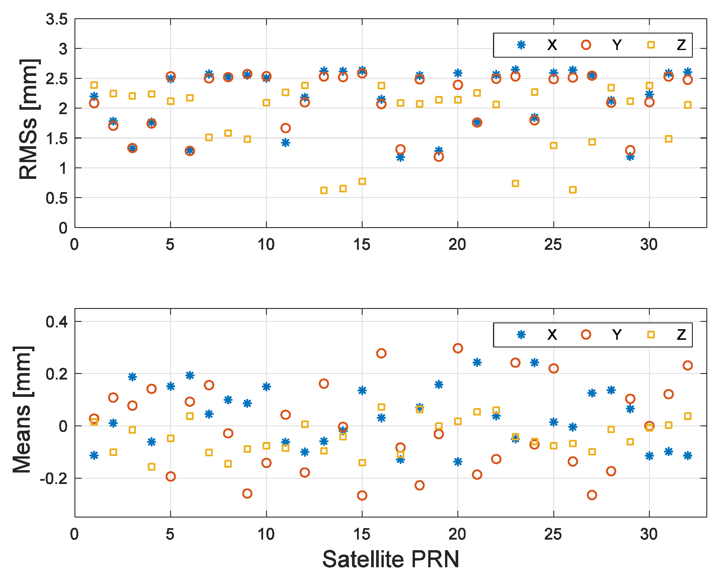
Figure 2.
The computed low-Earth orbit (LEO) satellite STP errors, with one-day precise reduced dynamic orbit products as the “true” value, with different sampling intervals: GOCE and GRACE (30-s intervals), and Jason-3 (60-s intervals).
Figure 2.
The computed low-Earth orbit (LEO) satellite STP errors, with one-day precise reduced dynamic orbit products as the “true” value, with different sampling intervals: GOCE and GRACE (30-s intervals), and Jason-3 (60-s intervals).

Figure 3.
The means (bottom) and RMSs (top) of the second-order, time-difference GPS clock errors, with one-day final 30-s IGS clock products as the “true” value, with 30-s sampling intervals.
Figure 3.
The means (bottom) and RMSs (top) of the second-order, time-difference GPS clock errors, with one-day final 30-s IGS clock products as the “true” value, with 30-s sampling intervals.

Figure 4.
Time-difference phase ionospheric residual (PIR), elevation angle, and satellite latitude for GPS PRN 5 at GOCE on 26 November 2009, with different sampling intervals. (a–c) First- or second-order time-difference PIRs for 1 s, 5 s, and 10 s, respectively; (d) GPS satellite elevation angle and GOCE satellite latitude.
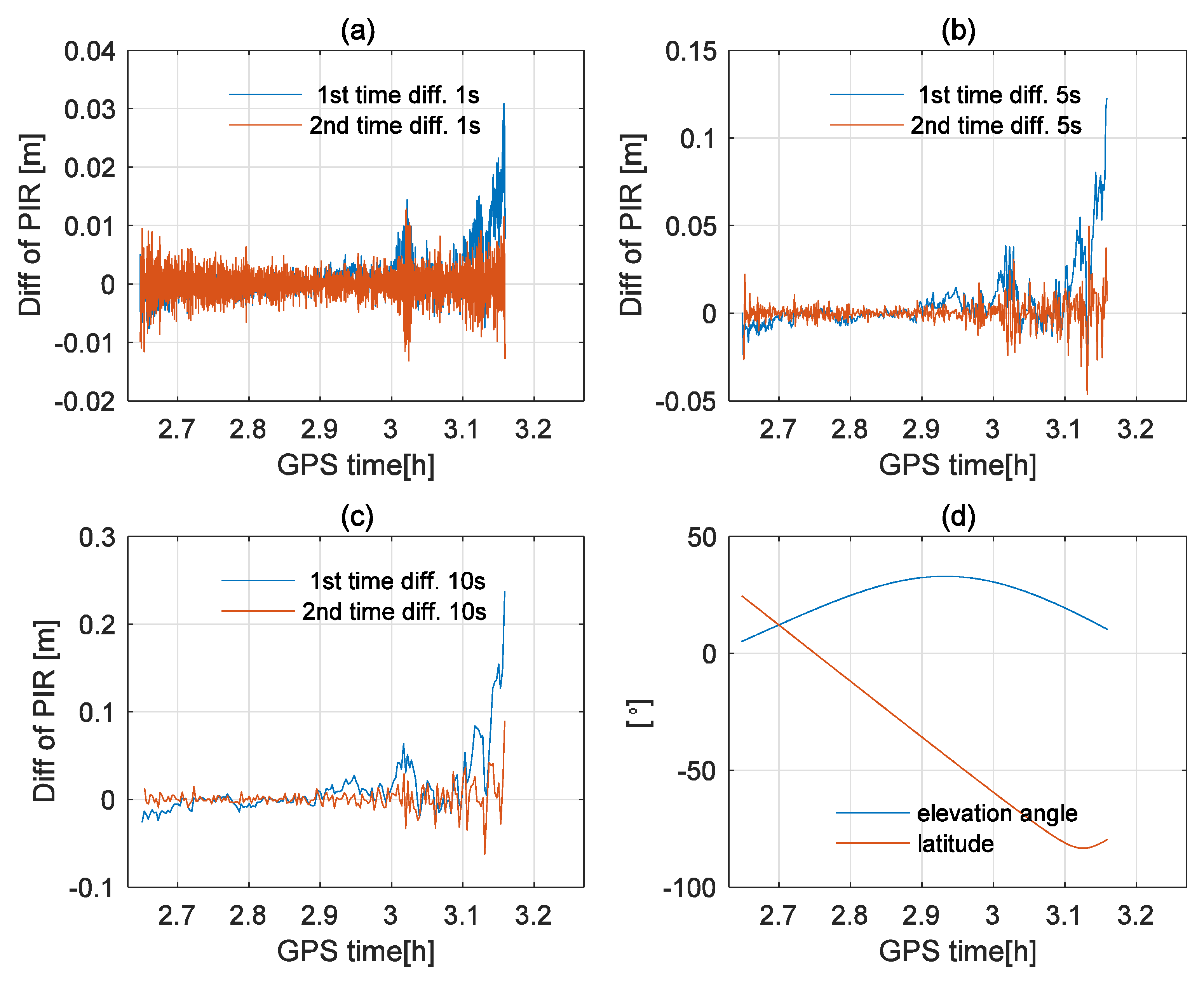
Figure 5.
Time-difference PIR, elevation angle, and satellite latitude for GPS PRN 19 at GOCE on 26 November 2009, with different sampling intervals. (a–c) First- or second-order time-difference PIRs for 1 s, 5 s, and 10 s, respectively; (d) GPS satellite elevation angle and GOCE satellite latitude.
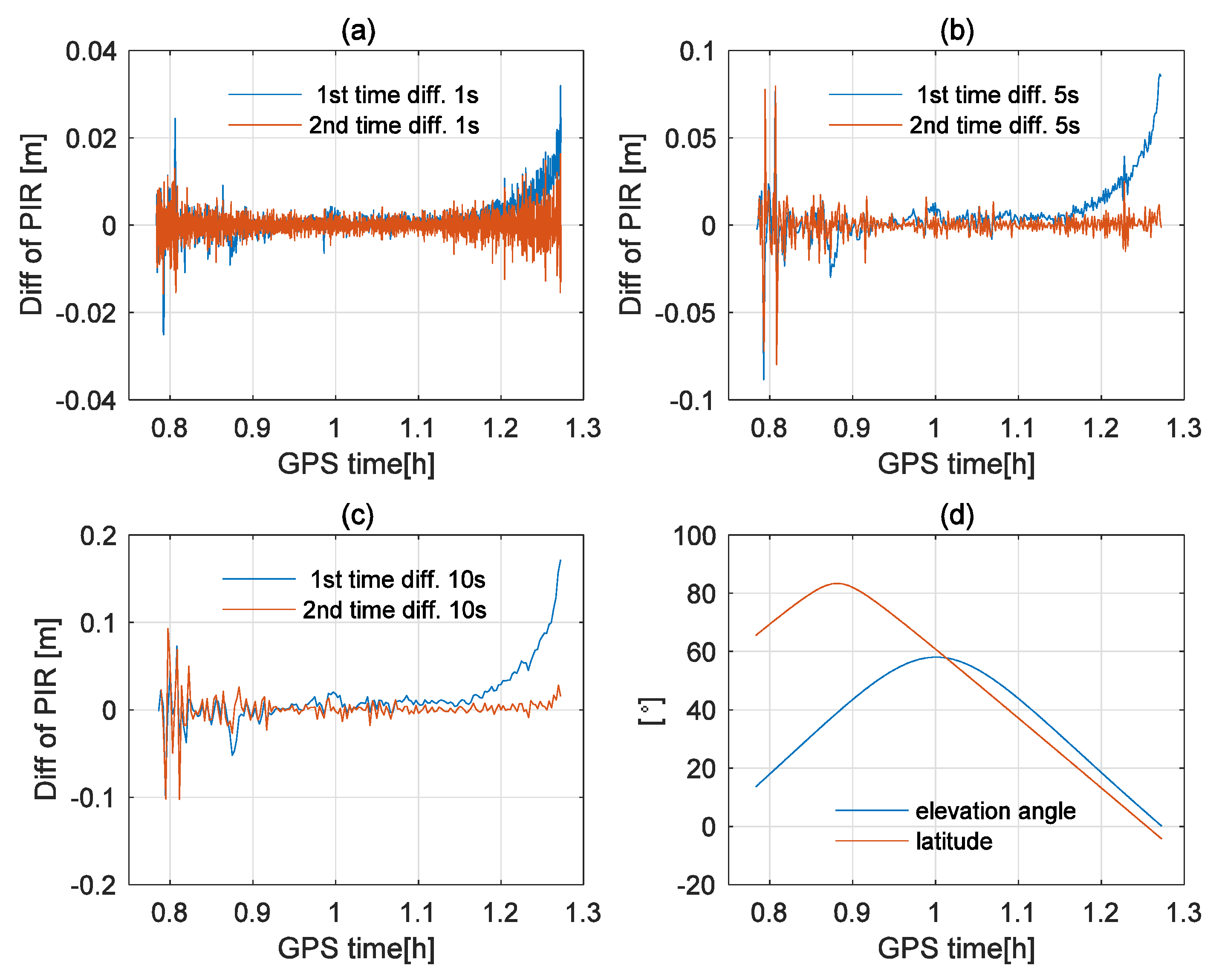
Figure 6.
GOCE satellite latitude, elevation, and second-order time-difference PIR (STPIR) (1 s) for GPS PRN 9 and PRN 22 on 21 November 2009.
Figure 6.
GOCE satellite latitude, elevation, and second-order time-difference PIR (STPIR) (1 s) for GPS PRN 9 and PRN 22 on 21 November 2009.
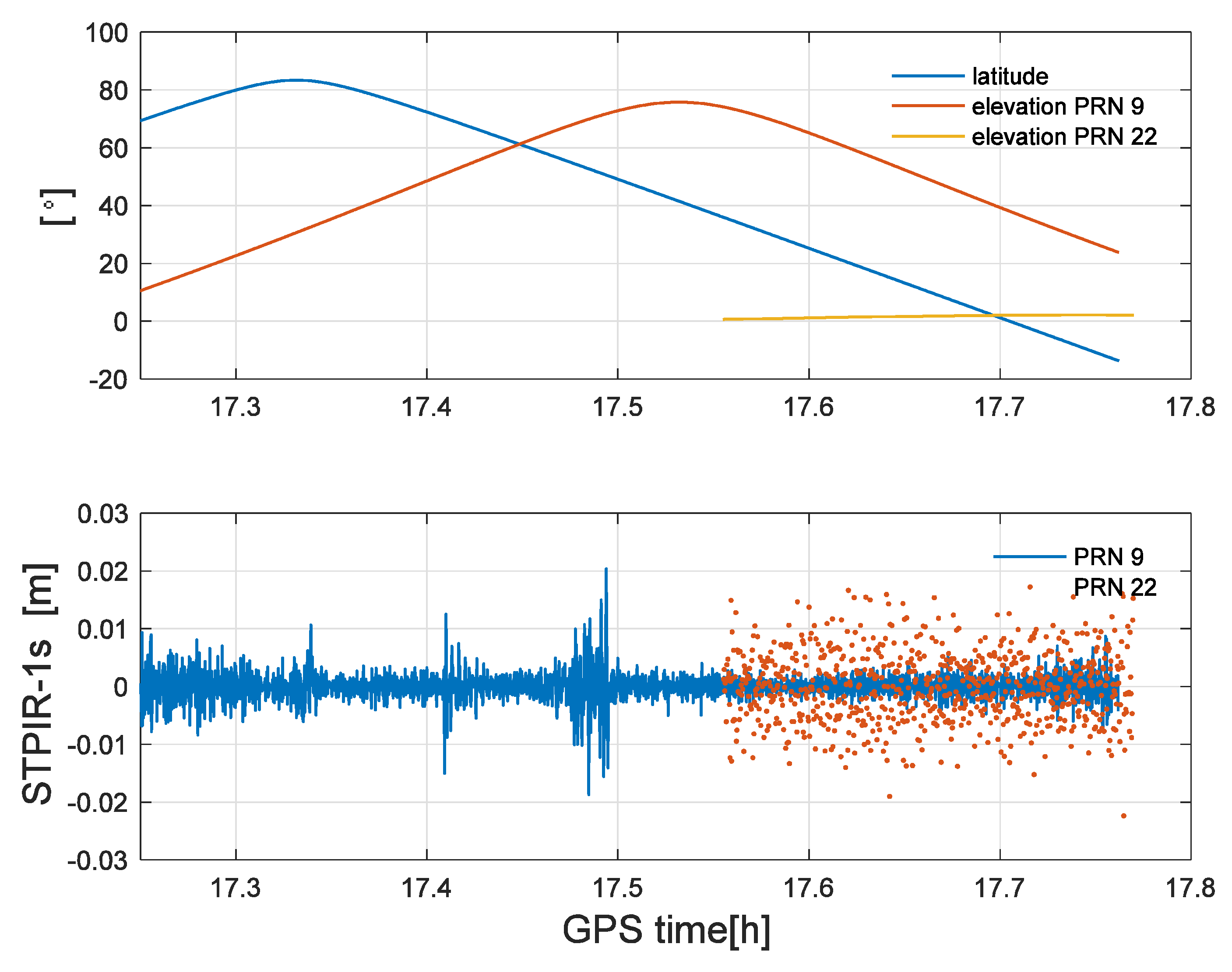
Figure 7.
Cycle slip detection results for GPS PRN 9 using STG combinations in Equations (10)–(13), denoted by (a–d), respectively, with simulated cycle slip pairs at GOCE on 21 November 2009.
Figure 7.
Cycle slip detection results for GPS PRN 9 using STG combinations in Equations (10)–(13), denoted by (a–d), respectively, with simulated cycle slip pairs at GOCE on 21 November 2009.
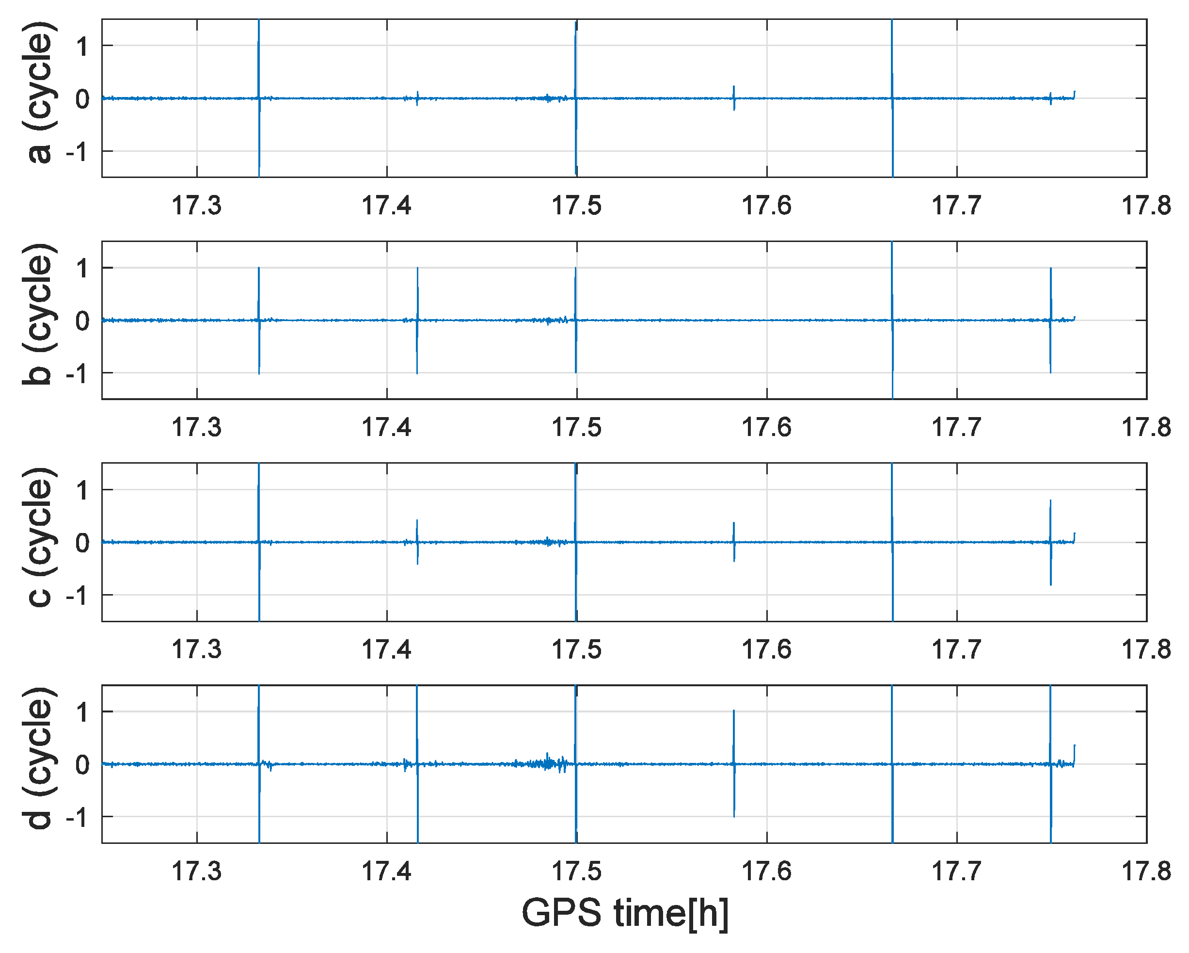
Figure 8.
Cycle slip detection results for GPS PRN 22 using STG combinations in Equations (10)–(13), denoted by (a–d), respectively, with simulated cycle slip pairs at GOCE on 21 November 2009.
Figure 8.
Cycle slip detection results for GPS PRN 22 using STG combinations in Equations (10)–(13), denoted by (a–d), respectively, with simulated cycle slip pairs at GOCE on 21 November 2009.


Table 1.
Acceleration accuracy requirements for different sampling intervals with an error at the 1-cm level.
Table 1.
Acceleration accuracy requirements for different sampling intervals with an error at the 1-cm level.
| Sampling Interval (s) | 1 | 5 | 10 | 30 |
|---|---|---|---|---|
| Acceleration error (ms−2) | 10−2 | 4 × 10⁻⁴ | 10−4 | 10−5 |
Table 2.
Ionospheric and geometric distance residuals with the different coefficients and .
| Equations | ||||
|---|---|---|---|---|
| Equation (10) | 1 | 0 | 0.3928 | |
| Equation (11) | 1 | −0.2833 | 0.2208 | |
| Equation (12) | 1 | −0.5 | 0.1765 | 0.5 |
| Equation (13) | 1 | 0 | 1 | 1 |
Table 3.
Several special cycle slip pairs (CSPs) and detected cycle slip values for the second-order time-difference geometry-free (STG) combinations.
Table 3.
Several special cycle slip pairs (CSPs) and detected cycle slip values for the second-order time-difference geometry-free (STG) combinations.
| CSPs | |||||
|---|---|---|---|---|---|
| 1 | 1 | 0.2208 | 0 | 0.3583 | 1 |
| 3 | 4 | −0.1169 | −1 | 0.4333 | 3 |
| 4 | 5 | 0.1039 | −1 | 0.7917 | 4 |
| 3 | 5 | −0.8961 | −2 | −0.2083 | 3 |
| 7 | 9 | −0.0130 | −2 | 1.2250 | 7 |
| 7 | 11 | −1.5714 | 4 | −0.0583 | 7 |
| 9 | 14 | −1.9091 | −5 | 0.0167 | 9 |
| 60 | 77 | 0 | −17 | 10.5917 | 60 |
Table 4.
Simulated special CSPs at GOCE satellite GPS observations.
| GPS Time | CSPs on PRN 9 | CSPs on PRN 22 |
|---|---|---|
| 5:20 p.m. | (5, 4) | -- |
| 5:25 p.m. | (3, 4) | -- |
| 5:30 p.m. | (3, 2) | -- |
| 5:35 p.m. | (1, 1) | (1, 1) |
| 5:40 p.m. | (9, 7) | (3, 4) |
| 5:45 p.m. | (4, 5) | (5, 4) |
Table 5.
Correct instances of detection and repair of cycle slips (in percentage) using STG methods for the GOCE GPS dataset above with sampling rates of 1-s, 5-s, and 10-s intervals for PRN 9 and PRN 22.
Table 5.
Correct instances of detection and repair of cycle slips (in percentage) using STG methods for the GOCE GPS dataset above with sampling rates of 1-s, 5-s, and 10-s intervals for PRN 9 and PRN 22.
| GPS Satellite | Interval(s) | Detection | Repair |
|---|---|---|---|
| PRN 9 | 1 | 100 | 100 |
| 5 | 100 | 99.9 | |
| 10 | 99.8 | 98.5 | |
| PRN 22 | 1 | 100 | 100 |
| 5 | 100 | 99.4 | |
| 10 | 99.7 | 97.6 |
© 2019 by the authors. Licensee MDPI, Basel, Switzerland. This article is an open access article distributed under the terms and conditions of the Creative Commons Attribution (CC BY) license (http://creativecommons.org/licenses/by/4.0/).
Share and Cite
MDPI and ACS Style
Wei, H.; Li, J.; Zhang, S.; Xu, X. Cycle Slip Detection and Repair for Dual-Frequency LEO Satellite GPS Carrier Phase Observations with Orbit Dynamic Model Information. Remote Sens. 2019, 11, 1273. https://doi.org/10.3390/rs11111273
AMA Style
Wei H, Li J, Zhang S, Xu X. Cycle Slip Detection and Repair for Dual-Frequency LEO Satellite GPS Carrier Phase Observations with Orbit Dynamic Model Information. Remote Sensing. 2019; 11(11):1273. https://doi.org/10.3390/rs11111273
Chicago/Turabian StyleWei, Hui, Jiancheng Li, Shoujian Zhang, and Xinyu Xu. 2019. "Cycle Slip Detection and Repair for Dual-Frequency LEO Satellite GPS Carrier Phase Observations with Orbit Dynamic Model Information" Remote Sensing 11, no. 11: 1273. https://doi.org/10.3390/rs11111273
Note that from the first issue of 2016, this journal uses article numbers instead of page numbers. See further details here.