Article

Using Single- and Multi-Date UAV and Satellite Imagery to Accurately Monitor Invasive Knotweed Species

1
Irstea, LESSEM Research Unit, University Grenoble Alpes, 2 rue de la Papeterie-BP 76, F-38402 St-Martin-d’Hères, France
2
Department of GIS and Remote Sensing, Institute of Botany of the Czech Academy of Sciences, 25243 Průhonice, Czech Republic
*
Author to whom correspondence should be addressed.
Remote Sens. 2018, 10(10), 1662; https://doi.org/10.3390/rs10101662
Submission received: 23 August 2018 / Revised: 29 September 2018 / Accepted: 18 October 2018 / Published: 20 October 2018

Abstract

:
Understanding the spatial dynamics of invasive alien plants is a growing concern for many scientists and land managers hoping to effectively tackle invasions or mitigate their impacts. Consequently, there is an urgent need for the development of efficient tools for large scale mapping of invasive plant populations and the monitoring of colonization fronts. Remote sensing using very high resolution satellite and Unmanned Aerial Vehicle (UAV) imagery is increasingly considered for such purposes. Here, we assessed the potential of several single- and multi-date indices derived from satellite and UAV imagery (i.e., UAV-generated Canopy Height Models—CHMs; and Bi-Temporal Band Ratios—BTBRs) for the detection and mapping of the highly problematic Asian knotweeds (Fallopia japonica; Fallopia × bohemica) in two different landscapes (i.e., open vs. highly heterogeneous areas). The idea was to develop a simple classification procedure using the Random Forest classifier in eCognition, usable in various contexts and requiring little training to be used by non-experts. We also rationalized errors of omission by applying simple “buffer” boundaries around knotweed predictions to know if heterogeneity across multi-date images could lead to unfairly harsh accuracy assessment and, therefore, ill-advised decisions. Although our “crisp” satellite results were rather average, our UAV classifications achieved high detection accuracies. Multi-date spectral indices and CHMs consistently improved classification results of both datasets. To the best of our knowledge, it was the first time that UAV-generated CHMs were used to map invasive plants and their use substantially facilitated knotweed detection in heterogeneous vegetation contexts. Additionally, the “buffer” boundary results showed detection rates often exceeding 90–95% for both satellite and UAV images, suggesting that classical accuracy assessments were overly conservative. Considering these results, it seems that knotweed can be satisfactorily mapped and monitored via remote sensing with moderate time and money investment but that the choice of the most appropriate method will depend on the landscape context and the spatial scale of the invaded area.

Graphical Abstract

1. Introduction

Biological invasions are usually seen as a major cause of global change that threatens biodiversity, ecosystem functioning, economies and human well-being [1]. As early monitoring and management of invasive alien plants (IAPs) is recognized as one of the most cost-efficient ways to tackle invasions [2], the elaboration of operational methods to quickly detect IAPs over large areas is particularly needed [3]. Consequently, an increasing number of studies have been published on the identification and mapping of IAPs using remote sensing technologies (for reviews, see: References [4,5]). Remote identification of plants was historically limited to trees and shrubs, but the rise of very high resolution (VHR) satellites and of Unmanned Aerial Vehicles (UAVs) with sub-metric to sub-decimetric spatial resolutions has led the way to the accurate mapping of herbaceous invaders [6]. VHR satellites have the advantage to cover large spaces of land on a regular basis while UAVs offer unmatched spatial and temporal resolutions for reasonable prices [7,8].
Japanese knotweed (Fallopia japonica; syn. Reynoutria japonica, Polygonum cuspidatum) and Bohemian knotweed (Fallopia × bohemica; syn. Reynoutria × bohemica, Polygonum × bohemicum) are among the most troublesome IAPs for land managers and conservationists in temperate regions of the world. Originally from eastern Asia, they have colonized countless areas of Europe, North America, Australia and New Zealand [9,10]. These highly competitive, fast-growing herbaceous plants are characterized by a wide environmental tolerance, strong regeneration capacities, important hybridization potential and both clonal and sexual reproduction [11,12]. Consequently, knotweeds are known to be extremely difficult to control, and their management has been the focus of numerous publications and reviews (e.g., References [13,14,15]). The annual economic cost of knotweed invasions is estimated to be around €2.3 billion in Europe [16] and above £165 million for the United Kingdom alone [17].
Improving detection and monitoring of knotweed populations could enhance control efficiency and decision making (c.f. [2,18,19]) and lead to a better understanding of their spatial dynamics [19,20], especially along their main dispersal axes—i.e., transportation corridors and rivers [21].
Unlike many woody species, the remote detection of herbaceous IAPs can be quite challenging as it usually requires very high spatial resolutions and implies that plants should have aggregated populations and not scattered growth habits [22,23,24]. Still, many studies report successful mapping of invasive herbaceous species using either hyperspectral sensors (e.g., References [25,26]), VHR satellite imagery (e.g., References [27,28,29]) or UAV imagery (e.g., References [30,31,32]). The number of possible approaches is quickly growing, but the detection remains highly species-specific [5,23]. Until recently, attempts to remotely detect knotweeds remained inconclusive (e.g., [33,34]). Müllerová et al. [35], however, used the extremely high spatiotemporal resolution of low-cost UAV imagery to track the phenological stages of the plant and finally reached classification accuracies suitable for operational applications with an image acquired in November, when the senescent plant differed most from the surrounding vegetation. However, since others failed to map knotweed with comparable images due to bad illumination and long projected shadows [36], and as this method is highly dependent on weather conditions and the duration of the senescence stage, alternative methods were needed.
An effective way to improve image classification results for a plant species that lacks a distinctive phenological response (e.g., distinct flowering organs) is to increase the number of variables used to describe this elusive response (e.g., spectral channels, texture features). Indeed, more variables mean more chances to uniquely specify the characteristic response of the plant. Hyperspectral images, with their many spectral bands, are commonly used for such a purpose [22]. For a long time, hyperspectral images had relatively coarse spatial resolutions [22,27]. The development of UAV-embedded hyperspectral sensors now offers very high spatial resolution, but these data are often difficult to handle for non-experts and would therefore be impractical for operational uses at the moment (c.f. [35]). Alternatively, the use of multi-date imagery to assess spectral differences in time has given promising results for IAPs detection [28,37], although it was unfruitfully tested for knotweeds [33]. The progress in the photogrammetry of UAV images also enables easy generation of 3D models that highlight the structure of vegetation [38,39], which may be helpful to distinguish plant growth forms.
In this applied study, our aim was to: (i) assess the potential of single- and multi-date variables for the success of knotweed detection from satellite and UAV imagery, (ii) evaluate the percentage cover of knotweed detected from both remote sensing platforms, and (iii) describe an easily reproducible classification procedure for the accurate mapping of knotweeds. Since remote sensing techniques are often too complex to be implemented by non-experts, we aimed to reduce the complexity by using commercial software that requires little training and data that are relatively easy to acquire and process. Our proposed methodology thus has the potential to become operational in practical management and ecological conservation.

2. Materials and Methods

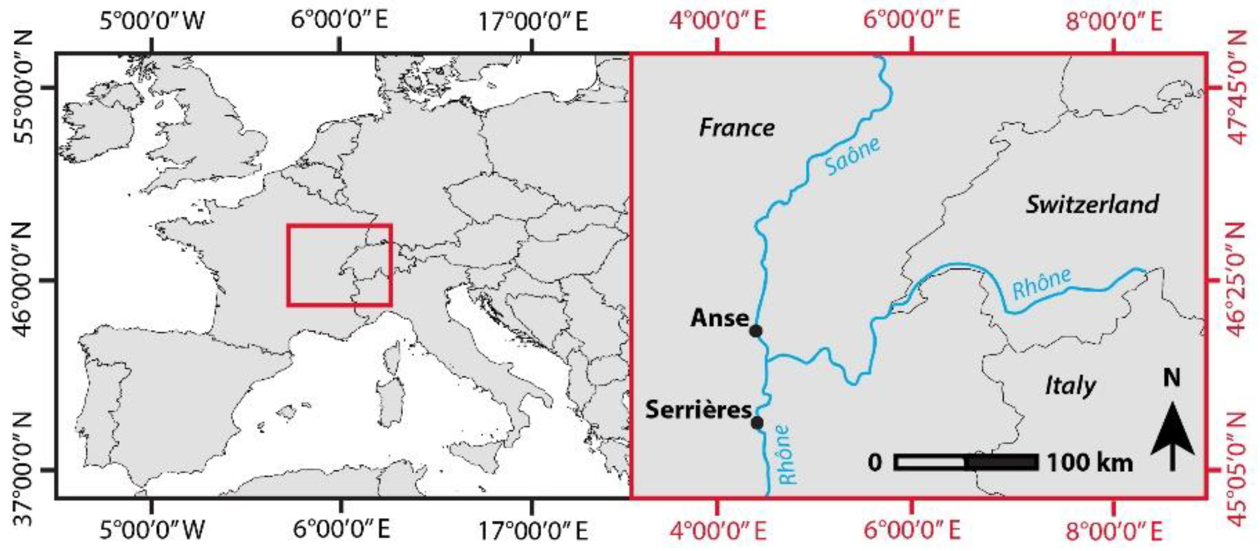
2.1. Study Sites and Image Acquisition

In this study, we worked on two different sites located in the floodplains of two major rivers of eastern France (Figure 1). For each site, a set of satellite and UAV images were acquired at three different time periods: spring, early summer and early fall (Table 1). Unfortunately, a crash of our UAV prevented us from acquiring the summer UAV images (the UAV was repaired in time for the early fall flights).
The satellite imagery consisted of Pleiades 1B PMS images with a 50 cm spatial resolution (the 2 m multispectral bands were pan-sharpened using the 50 cm panchromatic Pleiades bands), and a four-channel (RGB + NIR) spectral resolution.
The UAV images were obtained via a DS6 hexacopter UAV [DRONESYS, Saint Vincent de Mercuze, France]. The DS6 had a diameter of 80 cm for an approximate weight of 8 kg and could carry a payload of 3.5 kg. The UAV was equipped with two commercial cameras (Sony Alpha 7 with 24.3 Megapixels Full Frame Exmor CMOS Sensor and a Sonnar T* FE 35mm f/2.8 Zeiss lens). One camera was used to catch standard RGB bands while the other had been modified to acquire the near-infrared part of the spectrum (NIR): i.e., the built-in filter was replaced by MC Clear and Hoya R72 filters. The two cameras were embedded in a three-axis actively stabilized gimbal that controls for pitch and roll through the use of motors linked to AHRS sensors. The navigation and on-flight stability of the aircraft was managed by an A2 flight control system [DJI, Shenzhen, China]. Flight missions were pre-programmed and performed by the auto-pilot under the supervision of two pilots and a ground-control station. This low-cost flexible platform enabled the acquisition of 8 cm resolution imagery.
The Anse site (ca. 170 m a.s.l.) was located at the confluence of the Saône River and one of its tributaries, the Azergues River, whose banks are heavily invaded by knotweeds. The Anse Pleiades images covered an area of 213 ha comprising urban areas, croplands, major transportation infrastructure and semi-natural riparian environments. The UAV study area represented a 4.8 ha subset of the area covered by the Pleiades image and was characterized by highly heterogeneous riparian vegetation at the junction of the rivers. Some knotweed stands in the area are frequently mowed while others are unmanaged. The Serrières site (ca. 132 m a.s.l.) was located along the Rhône River. The Pleiades imagery covered an area of 263 ha composed of urban areas, various agricultural lands (vineyards, orchards and crops), forests and mostly-open riverbanks (recreational area) sporadically invaded by knotweeds. The UAV site covered an area of 7.1 ha and was restricted to an open riverbank zone of the site that hosted periodically mowed knotweed stands. This difference in management is important as mowing may greatly affect detection success. These sites were chosen because they differed in their landscape context and magnitude of invasion: i.e., the Anse site hosts a very large knotweed population composed of two huge monocultures and many stands of various sizes scattered across the landscape (the total area covered by knotweeds represents 45,772 m2), whereas the Serrières site is only colonized by some stands dispersed along the river (the total area covered by knotweeds represents 3361 m2).

2.2. Image Preprocessing

The Pleiades images were orthorectified on the Elevation 30 model and projected into the Lambert93 projection system based on the French RGF93 datum.
The two UAV cameras acquired regularly synchronized images with 85% forward and 70% side overlap during flight missions. We georeferenced and mosaicked the images with the photogrammetric software Photoscan v.1.2.6 (Agisoft LLC, St. Petersburg, Russia) using the Structure-from-Motion approach (SfM—[40,41]). SfM produces three-dimensional dense point clouds by identifying common features across scenes from the different angles of the images. Models are then transformed into absolute coordinates using Ground Control Points (GCPs) automatically identified in the images and measured on the ground by Post-Processed Kinematics-GNSS (Trimble Geoexplorer 6000—with mean deviation <0.3 m) to ensure georeferencing accuracy. Finally, the point clouds are segmented to generate Digital Surface Models (DSMs) and Digital Terrain Models (DTMs) that are in turn used to orthorectify the mosaics (for further details, see [38,40,41,42]), producing orthoimages with subdecimetric spatial resolutions.
The automatic generation of the DTMs and DSMs was based on two steps. Firstly, dense point clouds were divided into cells of a certain size (here, 10 m) in which the lowest points were detected. A triangulation of these points was then used to approximate a DTM. Here, to ensure that a maximum of “lowest points” were detected in the various landcovers of our study sites, we used additional UAV images acquired during the previous winter (when plants bore no leaves). Secondly, DSMs were extrapolated by a moving window that compared the remaining points of the clouds with the ground model to assess if their position differed from the ground by a given angle (here, 6°) and distance (here, 1 m) [41].
All data were further georeferenced using additional GCPs to ensure maximal correspondence between dates.

2.3. Classification Design and Variables

In order to evaluate the potential of single- and multi-date imagery for the detection and mapping of knotweeds, several classifications had to be compared. The idea was to assess the benefits of adding some “additional variables” extracted either from the image being classified itself (single-date analysis) or in comparison to an image acquired at another date (multi-date analysis) (Table 2). In other words, for each date and study site, we performed several classifications that differed only by the type of “additional variable” that was (or was not) included in the classifier algorithm.
There can be many different types of such “additional variables” (especially from multi-date images), such as differences in mean band values, texture, brightness, etc. For computational reasons, we only chose two kinds of variables easily computable by commercial software of image analysis: Bi-Temporal Band Ratios (BTBRs—multi-date information) and Canopy Height Models (CHMs—single- and/or multi-date information).
The BTBR was designed by Dorigo et al. [33] for the very purpose of characterizing the seasonal spectral behaviour of knotweeds by exploiting the phenological variation in the tissue’s chemistry and thus, the radiative responses in the red and green bands at different dates. However in their study, they only worked on two periods (spring and summer) and one of their aerial photographs did not have a NIR band. Since they recommended to always use the NIR band if possible, and since we worked on three different seasons, we developed a modified version of their BTBR:
MBTBR = ( N I R y / R x ) ( G y / G x ) ( N I R y / R x ) + ( G y / G x ) ,
where R, G and NIR stand for the mean values of the red, green and NIR bands, respectively (calculated for each image-object), while the suffix indicates the image the band is from [33]. Here, x always designated the image that was being classified, and y the image that was not being classified but from which ancillary information was derived. If classifications involved three different image dates (Table 2), three MBTBR indices were computed between each pair of images, where the suffix x designated the image that was being classified or the most recent image for the pair that did not include the image being classified.
The CHMs were built by subtracting the DTMs from the DSMs generated during the UAV imagery pre-processing. For this reason, CHMs were only used in the UAV image analysis, for which a CHM was computed for each date. In our analysis, we tested both single- and multi-date CHMs (Table 2). The latter gave information on species growth rates which may be useful to distinguish fast-growing species like knotweeds. Since it was an applied study investigating the potential of CHMs for knotweed detection and not a fundamental study seeking to evaluate the CHM generation process, only a preliminary accuracy assessment of the CHMs was performed (with a mean error in z-coordinates of 0.25 m calculated from 5 GNSS control-points per site and date of acquisition).

2.4. Classification Procedure

To produce the numerous classifications that had to be compared in this study, we decided to use an object-based approach because, unlike pixel-based methods that only account for the spectral information of images, it also enables the incorporation of scale-dependent structural and contextual information such as the texture, shape or topology of image-objects [43,44]. We thus carried out a multiresolution segmentation with a trial-and-error approach to find the best segmentation parameters for each image. Multiresolution segmentation is a region-merging technique that merges contiguous groups of pixels until a heterogeneity threshold (defined by parameters of scale, shape and colour) is crossed [45]. As emphasized by Müllerová et al. [35], knotweeds lack consistency in their shape and colour. Consequently, we had to operate a very fine segmentation to isolate knotweed-objects from the surrounding background and other plant species, creating tens of thousands of image-objects.
To classify the image-objects, we used the machine learning algorithm Random Forest (RF) that combines multiple classification trees [46]. RF is a non-parametric classifier based on “bagging” (for bootstrap aggregating) that only uses random subsets of training objects and input variables to make decisions, offering several advantages: It is easy to parametrize; computationally efficient; and it is robust to overfitting, correlation between variables, and unbalanced training samples [46,47]. To help the algorithm, we decided to create several thematic classes apart from knotweeds (e.g., water, buildings, trees), that were ultimately merged to only retain three classes: knotweed, cut knotweed and other. For September UAV classifications in Anse, an additional class of knotweed was created (called island knotweed) because some knotweeds located on a river shoal had a different appearance than the other stands (probably because they grew on a seasonally submerged shoal).
To train the RF algorithm, training objects visible at every acquisition date were sampled for each class. Since some classes were more abundant than others and since the size of images differed between sites and image-type (satellite or UAV), we could not reach an equal number of samples per class. However, we ensured that each class had between 5 and 30% of its surface selected for training (for knotweed classes, the values were between 25 and 30% to ensure globally similar sample sizes across the various classifications).
As we were interested in the effect of MBTBRs and CHMs, we used exactly the same object features (except for, when relevant, the addition of MBTBRs and CHMs) as in Müllerová et al. [35] to be able to compare our results with theirs. These image-object features were: NDVI, statistics on band values (mean, maximum, minimum and normal and circular standard deviations), contrast to neighbouring pixels, geometrical features (area, border length, length/width ratio, asymmetry and compactness) and texture-based metrics (GLCM features of homogeneity, contrast, dissimilarity and entropy in all directions).
All steps of classification were performed in eCognition Developer v.8.9.1 [48].

2.5. Validation and Accuracy Assessment

Four field campaigns in Serrières and six in Anse were conducted in 2016 to cover both study sites in their entirety and thus map all knotweed stands using high-precision GNSS. However, since the ultra-high resolution of UAV imagery often exceeds the precision of the highly time-consuming GNSS measurements [24,49], all mapped polygons were manually corrected through photo-interpretation to ensure sufficient precision matching between the validation datasets and the classification results. Still, many unwanted changes (e.g., shadows, hidden parts of knotweed populations) were displayed across multi-date images due to the imagery characteristics (e.g., timing of acquisition, camera angles, weather conditions), positioning errors, and landscape modifications (e.g., construction, floods, growing vegetation). Therefore, we decided to create an exclusive validation dataset for each date. We also separated our datasets between “total” and “visible” knotweed populations by manually modifying the validation polygons to remove the parts of knotweed populations that were hidden by trees.
Validation was performed on all knotweed surfaces independent of the training samples (we mapped every square metre of knotweed cover and not just samples), and we computed Producer’s Accuracies (PA; accounting for errors of omission) and User’s Accuracies (UA; accounting for errors of commission) to evaluate and compare results [50]. Therefore, PA was computed by dividing the correctly classified cover area of the validation dataset (in m2) by the total cover area of knotweed (minus the 25–30% of cover used as training samples), and UA was computed by dividing the correctly classified cover area of knotweed by the total area classified as knotweed [50]. Since knotweeds represented only a small proportion of the total study areas and since we were not interested by other classes than knotweeds, general agreement metrics (e.g., Kappa index, Overall Accuracy) were not computed as they would have been misleading [51,52,53].
As already mentioned, working with multi-date imagery increases sources of error. In remote sensing, mixed-objects and misregistration issues are usually unavoidable [54,55], but they are enhanced with every addition of data [55]. Consequently, in order to assess the amount of knotweed cover that is missed (i.e., amount of PA reduction) due to these “multi-data” issues, we applied “buffer” boundaries around knotweed predictions to artificially widen them. Predicted objects were thus validated using two types of boundaries, a “crisp” boundary and “buffer” boundaries of two sizes: 2-pixels and 10-pixels (i.e., 16 cm and 80 cm, and 1 m and 5 m for the UAV and the Pleiades images, respectively). In other words, for a 10-pixel “buffer” boundary validation of a UAV classification, any objects within 80 cm of an object predicted as knotweed were classified as knotweed as well. Since we used “surfaces” for validation, “buffer” boundaries necessarily affected UAs (rates of “true-positive” predictions) but not in terms of occurrences (a false prediction is false regardless of its size).
All steps of validation were performed in ArcGIS 10.3 [56].

3. Results

We only present the results for the knotweed populations that were visible from the sky. Indeed, 48.8% and 9% of the total knotweed cover was located under the tree canopy in Anse and Serrières, respectively (and was thus invisible on the images), and was therefore not taken into account. Additionally, due to fresh cutting of knotweed stands at the Serrières site just before several image acquisitions (i.e., all Pleiades images and the fall ones for the UAV), classifications of both Pleiades data and UAV autumn datasets resulted in accuracies below 40% and are thus not presented here.
For the “crisp” Pleiades results (Table 3), the accuracies obtained were relatively weak except for the surprisingly high UA’s for the cut knotweed class in the fall classifications (the other results for this class were globally weak; Table S1). For the knotweed class, the results are quite comparable between the different spring Pleiades classifications, but using MBTBRs mildly improved UAs. The use of MTBRs also globally improved both PAs and UAs for the fall classifications (the best PA/UA was 61/34% for the Fall-Summer classification).
The UAV classifications reached much higher accuracies than the Pleiades ones (Table 3). In Anse, CHMs and MBTBRs always improved PAs for the knotweed class and usually improved UAs but with less consistency (Table 3). For the UAV-site of Serrières, the addition of CHMs and MBTBRs only had a mildly positive effect on the already high PAs of the knotweed class and seemingly no effect on the low PAs of the cut knotweed class (Table S2). On the other hand, it led to a very strong increase in UA for both classes at Serrières (Table 3). Except for the cut knotweed class at Serrières and knotweed’s UA for the spring classification in Anse, all the best results were obtained from using multi-date classification (usually with both CHMs and MBTBRs), and adding CHMs (both single- and multi-date) always improved PAs.
The use of the “buffer” boundaries strongly increased accuracies for both Pleiades and UAV classifications, with PAs often exceeding 80 or even 90% (Table 3). This indicates that, in most cases, the classifier detected the majority of knotweed stands and that the missing parts of the knotweed cover are mostly located on the edges of the detected stands (Figure 2).

4. Discussion

In this study, we assessed the potential of single-date (i.e., spectral, textural and contextual data, CHMs) and multi-date information (i.e., CHMs and MBTBRs) extracted from imagery acquired at different resolutions and time-periods for the detection and mapping of invasive knotweeds with accessible commercial software to make the workflow applicable in ecological conservation. The results show that, for a moderate time and cost investment, knotweeds can now be accurately mapped for operational uses at different spatial scales especially using MBTBRs and UAV-generated CHMs, if not hidden under the canopy of trees or freshly cut. However, the quality of detections strongly depends on the landscape context. To the best of our knowledge, it is the first time UAV-generated CHMs are used to detect IAPs, and our study clearly shows the potential of such an approach.
To date, the literature on knotweed detection using remote sensing is very limited as knotweeds have proven to be quite difficult to distinguish from other plant species. The first attempts were made on aerial photographs and VHR satellite imagery but these studies did not provide quantitative accuracy assessments [34,57], or failed to map the plant due to insufficient population sizes [58]. Dorigo et al. [33], introducing the use of BTBR to quantify the temporal differences in the spectral response of knotweeds, only obtained a PA/UA of 61/7% with their aerial orthophoto and their pixel-based approach using the RF classifier. More recently, Michez et al. [36] tried to map the distribution of three IAPs (including knotweeds) using an object-based approach on UAV orthophotos. They admitted failing at reaching satisfying results, notably because their late-fall images included too many projected shadows [36]. Müllerová et al. [35], on the other hand, compared UAV and Pleiades images acquired at different dates and classified with different algorithms to evaluate the best trade-offs between spectral, spatial and temporal resolutions for operational applications. Their pixel-based analysis gave the best PAs/UAs of 74/95% for a July Pleiades image (50 cm) with a RF classifier, and of 82/83% for a November UAV image (which allowed them to detect some under-canopy knotweed populations) resampled to a 50 cm spatial resolution and classified with a Maximum Likelihood classifier. For the satellite analysis, they consequently obtained better accuracies than our best “crisp” Pleiades results. With the UAV imagery, however, our best “crisp” PA results were comparable to (Anse site) or outperformed (Serrières) the results of Müllerová et al. [35]. Compared to the late autumn imagery used in Müllerová et al. [35], using images from late-spring/early-fall provides opportunities for better image acquisition due to an extended season for collection and better weather conditions. Our proposed methodology therefore enables the accurate mapping of knotweeds any time during the growing season, which could be valuable for practical management applications.
The mentioned differences in accuracies among the study sites are likely due to their landscape context. Both single-and multi-date detection of knotweeds is easier in open landscapes such as the Serrières site (i.e., a riverside recreational open lawn), where the plant grows in well-shaped stands distinct from the background. In more complex landscapes, where the nature and size of real objects is highly heterogeneous, classification errors due to mixed-pixels or mixed-objects increase [59]. Detection of knotweed stands in semi-natural riparian areas like Anse and the Czech site of Müllerová et al. [35] was, therefore, likely impeded by the heterogeneous cover that included many shadows, mingled-vegetation, and growing shrubs and trees. Fortunately, knotweeds do not commonly grow inside closed forests [60]; large forest populations like the one in Anse being extremely rare. Our results indicate that in such landscapes dominated by a highly heterogeneous vegetation cover, the use of CHMs (single- or multi-date) brings substantial accuracy improvements. CHMs are rarely used to map IAPs, especially herbaceous species (but some authors have used LiDAR-based CHMs to map woody plants (see Reference [61]). It is surprising since CHMs, whether single- or multi-date, should be particularly useful to reduce confusion between trees (or shrubs) and fast-growing herbaceous species (e.g., [62,63]). This is supported in our study, as the accuracy gained from the CHMs at the Serrières site, which was composed mostly of grass and fast-growing forbs like knotweeds or reeds, was weaker than at the wooded site of Anse (Table 3). Since it is the first time UAV-generated CHMs are used to map the distribution of an IAP and since no accuracy assessment of the CHMs themselves has been made, errors in CHMs likely exist and improvements in the methods can certainly be undertaken. Nevertheless, CHMs improved results in all of our classifications (Table 3).
Our “buffer” boundary results outperformed by far those obtained by any other study. While it is reasonable to assume that “buffer” boundaries partly included knotweed cover that would never have been classified as such by the classifier (i.e., only by chance), it also likely compensated for a substantial portion of the mis-registrations and mixed-objects at the edge or within knotweed stands due to the use of multi-date imagery (Figure 3). Such inevitable errors are indeed enhanced with every addition of data (e.g., image, spectral band, CHM). In Figure 3a, for instance, visible knotweed cover changes across dates due to floods or long projected shadows. In Figure 3b,c, image-objects circled in red are homogeneous on the spring image but not on the fall one because of the growing vegetation and the spectral and positional registration inaccuracies between images. Such image-objects (all knotweeds) would have different heterogeneous spectral or textural responses, and would thus probably be classified differently in multi-date classification, leading to patchy detection and mapping of numerous image-objects at the edge or within stands. In other words, even if CHMs and MBTBRs improve discrimination of image-objects that are homogeneous across all dates, they artificially reduce the accuracy of image-objects that are heterogeneous across dates because they are too different from the training samples chosen on the homogeneous objects. CHMs derived from SfM procedure also show imprecisions in areas of very dense canopy (average XYZ errors ranging from 3 to 14 cm) due to the lack of visible ground, leading to some inaccuracies in CHMs. Mis-registrations were further enhanced by the difficulty of finding suitable GCPs across imagery in semi-natural areas due to the lack of “fixed” elements: e.g., constructions, rocks. These assumptions are supported by the fact that, even with weak “crisp” PAs, most of the 10-pixels “buffer” PAs reached or exceeded 90–95%. This means that in most cases, the vast majority of the “omitted” knotweed cover lies in the direct vicinity of detected stands (as shown in Figure 2), but that “crisp” accuracy assessments are too conservative to capture the full extent of knotweed image-objects. On balance, “buffer” boundaries may be more useful for end-users primarily interested in PAs, such as land managers or conservation scientists, while the information given by “buffer” boundaries may be less relevant for end-users whose purpose is to build prediction models as they may be more interested in UAs.
Our “buffer” boundary results actually provide useful information to the end-user by rationalizing PAs that would otherwise be unfairly low for practical use; see Reference [54]. Using such an approach lowers the likelihood of knotweed omission that is of interest for eradication measures. Moreover, these “buffer” boundaries may well represent reasonable distances of prospection during field surveys, i.e., end-users monitoring/eradicating knotweed stands using remote sensing predictions will most probably include a few centimetres to metres around the predicted location to their survey. To illustrate, a PA/UA of 98/80% with an 80 cm “buffer” boundary (i.e., like our Spring-biCHM classification in Serrières) means that if one goes and checks just 80 cm around every location predicted as knotweed, one will actually find 98% of the knotweed cover of the study area visible from the sky and only get 20% of “false-positive” predictions (adding a buffer zone around a false prediction does not make it any truer, and therefore changes of UA due to “buffer” boundaries are not relevant).
The choice of the most appropriate approach and imagery, therefore, varies with the purpose of the classification (e.g., land management, biodiversity conservation, research on biological invasions), the type of landscape, and the scale of the target area. For regional scales, the use of VHR satellite imagery is the only reasonable option. In such a case, the pixel-based approach of Müllerová et al. [35] may be more appropriate than object-based classifications because at this resolution, knotweed stands lack distinctive features. Still, adding MBTBRs in the classification workflow could likely improve the results. If single-date analysis is chosen, the image should preferably be acquired during early summer when knotweeds are at their full-height and projected shadows are the shortest (e.g., Figure 3a) or, if the weather allows it, at the late autumn senescent stage, as suggested by Müllerová et al. [35]. At the local scale, for simple and open landscapes, UAV single-date images could work well, but good results can also be achieved with spring images with single- or multi-date analyses (Table 3). For more complex and heterogeneous landcovers, the use of at least two-date MBTBRs and/or CHMs is strongly recommended if images cannot be acquired during the senescence stage where knotweeds are most distinctive [35], which is likely in regions where autumns are characterized by cloudy conditions. CHMs should be particularly useful in heterogeneous vegetation to help distinguish between herbaceous and woody species [62,63].

5. Conclusions

We showed that the highly problematic knotweeds can be accurately mapped (i.e., false positive and true positive error rates often below 10–15%) from both satellite and UAV imagery, particularly when using multi-date band ratios and Canopy Height Models (CHMs). The proposed methodology provides a powerful tool in invasive alien plants (IAPs) management, with high accuracy and a straight-forward approach assuring its operational use. Proposed automated detection of one of the most problematic IAP in Europe and North America can increase the effectiveness of eradication measures as well as reduce the costs of expensive field campaigns, enabling early detection, regular monitoring and assessment of control measures. The results showed that it is possible to detect very small knotweed stands as long as they cover areas larger than 4–5 pixels and are visible from above. However, plants growing under the tree canopy, or that are freshly cut, remain excessively hard to detect.
Regardless of the chosen method, end-users should be aware of both limitations and improvement perspectives. The pre-processing procedure of UAV images is relatively straightforward but still requires some technical expertise and, as a new technique, is undergoing rapid development (see References [38,40]). UAVs are also sensitive to weather hazards and constraining legal regulations [7]. For both satellite and UAV imagery, the quality of imagery influences the choice of the data to be classified and the number of classes to be created. Wrong timing of data acquisition is a frequent issue (e.g., if the target species has been freshly cut or eradicated), though detection may still be feasible (e.g., if knotweeds had some time to regrow). On the other hand, easy improvements of accuracy could be obtained from masking out unlikely locations using GIS expert-systems, improving surface reflectance calibration, and using multi-date segmentation and texture analysis (at the expense of computational time). Incorporating UAV-embedded LiDAR to account for errors in z-coordinates and thus improve the accuracy of CHMs could also likely increase detection accuracies. Finally, another promising approach would be the use of hyperspectral imagery. For many years, the cost and spatial resolution of hyperspectral satellite or airborne imagery was unfit for the detection of herbaceous species. However, UAV-borne hyperspectral solutions are now emerging and give interesting results for the monitoring of plants [64,65]. Further research on the use of such technologies for knotweed detection should certainly be undertaken although their expertise requirements would be a deterrent for many potential end-users.

Supplementary Materials

The supplementary materials are available online at https://www.mdpi.com/2072-4292/10/10/1662/s1.

Author Contributions

Conceptualization, F.-M.M., J.M. and L.B.; Formal analysis, F.-M.M. and L.B.; Funding acquisition, A.E.; Methodology, F.-M.M., J.M., L.B. and V.B.; Project administration, F.D. and A.E.; Resources, V.B.; Software, F.-M.M. and L.B.; Supervision, F.D. and A.E.; Validation, J.M.; Writing—original draft, F.-M.M.; Writing—review & editing, J.M., L.B., F.D., V.B. and A.E.

Funding

This work was funded by Irstea, the Dynarp-ITTECOP project, and project PHC Barrande 2018 no. 40617UG. This work was also supported by public funds received in the framework of GEOSUD, a project (ANR-10-EQPX-20) of the program “Investissements d’Avenir” managed by the French National Research Agency. Jana Müllerová was supported by a long-term research development project no. RVO 67985939 and projects LTC18007 and 8J18FR021.

Acknowledgments

We are grateful to Manon Racle, Marine Stromboni, Eric Mermin, Frédéric Ousset and Joseph Brůna for their help on data acquisition and processing, and to Kelsey Elwood for her English proofreading of the manuscript. We also thank the three anonymous reviewers for their helpful comments on the manuscript.

Conflicts of Interest

The authors declare no conflict of interest.

References

  1. Vilà, M.; Ibáñez, I. Plant invasions in the landscape. Landsc. Ecol. 2011, 26, 461–472. [Google Scholar]
  2. Holden, M.H.; Nyrop, J.P.; Ellner, S.P. The economic benefit of time-varying surveillance effort for invasive species management. J. Appl. Ecol. 2016, 53, 712–721. [Google Scholar] [CrossRef]
  3. Byers, J.E.; Reichard, S.; Randall, J.M.; Parker, I.M.; Smith, C.S.; Lonsdale, W.; Atkinson, I.; Seastedt, T.; Williamson, M.; Chornesky, E. Directing research to reduce the impacts of nonindigenous species. Conserv. Biol. 2002, 16, 630–640. [Google Scholar] [CrossRef]
  4. Huang, C.Y.; Asner, G.P. Applications of remote sensing to alien invasive plant studies. Sensors 2009, 9, 4869–4889. [Google Scholar] [CrossRef] [PubMed]
  5. Bradley, B.A. Remote detection of invasive plants: A review of spectral, textural and phenological approaches. Biol. Invasions 2014, 16, 1411–1425. [Google Scholar] [CrossRef]
  6. Müllerová, J.; Brůna, J.; Dvořák, P.; Bartaloš, T.; Vítková, M. Does the data resolution/origin matter? Satellite, airborne and UAV imagery to tackle plant invasions. Int. Arch. Photogramm. Remote Sens. Spat. Inf. Sci. 2016, 41, 903–908. [Google Scholar]
  7. Dvořák, P.; Müllerová, J.; Bartaloš, T.; Brůna, J. Unmanned aerial vehicles for alien plant species detection and monitoring. Int. Arch. Photogramm. Remote Sens. Spat. Inf. Sci. 2015, XL-1/W4, 83–90. [Google Scholar]
  8. Remondino, F.; Barazzetti, L.; Nex, F.; Scaioni, M.; Sarazzi, D. UAV photogrammetry for mapping and 3d modeling-current status and future perspectives. Int. Arch. Photogramm. Remote Sens. Spat. Inf. Sci. 2011, 38, C22. [Google Scholar] [CrossRef]
  9. Alberternst, B.; Böhmer, H. NOBANIS: Invasive Alien Species Fact Sheet—Reynoutria japonica. Online Database of the European Network on Invasive Alien Species. Available online: www.nobanis.org (accessed on 12 January 2018).
  10. Bailey, J.; Wisskirchen, R. The distribution and origins of Fallopia × bohemica (Polygonaceae) in Europe. Nord. J. Bot. 2006, 24, 173–199. [Google Scholar] [CrossRef]
  11. Bailey, J.P.; Bímová, K.; Mandák, B. Asexual spread versus sexual reproduction and evolution in Japanese knotweed s.l. Sets the stage for the “battle of the clones”. Biol. Invasions 2009, 11, 1189–1203. [Google Scholar] [CrossRef]
  12. Buhk, C.; Thielsch, A. Hybridisation boosts the invasion of an alien species complex: Insights into future invasiveness. Perspect. Plant Ecol. Evol. Syst. 2015, 17, 274–283. [Google Scholar] [CrossRef]
  13. Child, L.; Wade, M. The Japanese Knotweed Manual; Packard Publishing Limited: Chichester, UK, 2000; Volume 1, 123p, ISBN-10 1 85341 127 2. [Google Scholar]
  14. Bashtanova, U.B.; Beckett, K.P.; Flowers, T.J. Review: Physiological approaches to the improvement of chemical control of Japanese knotweed (Fallopia japonica). Weed Sci. 2009, 57, 584–592. [Google Scholar] [CrossRef]
  15. McHugh, J.M. A Review of Literature and Field Practices Focused on the Management and Control of Invasive Knotweed. 2006, pp. 1–32. Available online: http://citeseerx.ist.psu.edu/viewdoc/download?doi=10.1.1.512.6014&rep=rep1&type=pdf (accessed on 23 August 2018).
  16. Kettunen, M.; Genovesi, P.; Gollasch, S.; Pagad, S.; Starfinger, U.; ten Brink, P.; Shine, C. Technical Support to EU Strategy on Invasive Alien Species (IAS); Assessment of the Impacts of IAS in Europe and the EU (Final Module Report for the European Commission); Institute for European Environmental Policy (IEEP): Brussels, Belgium, 2009; 44p. [Google Scholar]
  17. Williams, F.; Eschen, R.; Harris, A.; Djeddour, D.; Pratt, C.; Shaw, R.; Varia, S.; Lamontagne-Godwin, J.; Thomas, S.; Murphy, S. The Economic Cost of Invasive Non-Native Species on Great Britain; CABI Proj No. VM10066; CABI: Oxfordshir, UK, 2010; Volume 9, 199p. [Google Scholar]
  18. Meier, E.S.; Dullinger, S.; Zimmermann, N.E.; Baumgartner, D.; Gattringer, A.; Hülber, K. Space matters when defining effective management for invasive plants. Divers. Distrib. 2014, 20, 1029–1043. [Google Scholar] [CrossRef]
  19. Fox, J.C.; Buckley, Y.M.; Panetta, F.; Bourgoin, J.; Pullar, D. Surveillance protocols for management of invasive plants: Modelling Chilean needle grass (Nassella neesiana) in Australia. Divers. Distrib. 2009, 15, 577–589. [Google Scholar] [CrossRef]
  20. Pyšek, P.; Hulme, P.E. Spatio-temporal dynamics of plant invasions: Linking pattern to process. Ecoscience 2005, 12, 302–315. [Google Scholar] [CrossRef]
  21. Tiébré, M.-S.; Saad, L.; Mahy, G. Landscape dynamics and habitat selection by the alien invasive Fallopia (Polygonaceae) in Belgium. Biodivers. Conserv. 2008, 17, 2357–2370. [Google Scholar] [CrossRef]
  22. Lass, L.W.; Prather, T.S.; Glenn, N.F.; Weber, K.T.; Mundt, J.T.; Pettingill, J. A review of remote sensing of invasive weeds and example of the early detection of spotted knapweed (Centaurea maculosa) and babysbreath (Gypsophila paniculata) with a hyperspectral sensor. Weed Sci. 2005, 53, 242–251. [Google Scholar] [CrossRef]
  23. Mulla, D.J. Twenty five years of remote sensing in precision agriculture: Key advances and remaining knowledge gaps. Biosyst. Eng. 2013, 114, 358–371. [Google Scholar] [CrossRef]
  24. Müllerová, J.; Pergl, J.; Pyšek, P. Remote sensing as a tool for monitoring plant invasions: Testing the effects of data resolution and image classification approach on the detection of a model plant species Heracleum mantegazzianum (giant hogweed). Int. J. Appl. Earth Obs. Geoinf. 2013, 25, 55–65. [Google Scholar] [CrossRef]
  25. Fernandes, M.R.; Aguiar, F.C.; Silva, J.M.; Ferreira, M.T.; Pereira, J.M. Optimal attributes for the object based detection of giant reed in riparian habitats: A comparative study between airborne high spatial resolution and WorldView-2 imagery. Int. J. Appl. Earth Obs. Geoinf. 2014, 32, 79–91. [Google Scholar] [CrossRef]
  26. Guo, Y.; Graves, S.; Flory, S.L.; Bohlman, S. Hyperspectral measurement of seasonal variation in the coverage and impacts of an invasive grass in an experimental setting. Remote Sens. 2018, 10, 784. [Google Scholar] [CrossRef]
  27. Walsh, S.J.; McCleary, A.L.; Mena, C.F.; Shao, Y.; Tuttle, J.P.; González, A.; Atkinson, R. Quickbird and Hyperion data analysis of an invasive plant species in the Galapagos Islands of Ecuador: Implications for control and land use management. Remote Sens. Environ. 2008, 112, 1927–1941. [Google Scholar] [CrossRef]
  28. Ouyang, Z.T.; Gao, Y.; Xie, X.; Guo, H.Q.; Zhang, T.T.; Zhao, B. Spectral discrimination of the invasive plant Spartina alterniflora at multiple phenological stages in a saltmarsh wetland. PLoS ONE 2013, 8, e67315. [Google Scholar] [CrossRef] [PubMed]
  29. Ouyang, Z.T.; Zhang, M.Q.; Xie, X.; Shen, Q.; Guo, H.Q.; Zhao, B. A comparison of pixel-based and object-oriented approaches to VHR imagery for mapping saltmarsh plants. Ecol. Inf. 2011, 6, 136–146. [Google Scholar] [CrossRef]
  30. Hill, D.J.; Tarasoff, C.; Whitworth, G.E.; Baron, J.; Bradshaw, J.L.; Church, J.S. Utility of unmanned aerial vehicles for mapping invasive plant species: A case study on yellow flag iris (Iris pseudacorus L.). Int. J. Remote Sens. 2017, 38, 2083–2105. [Google Scholar] [CrossRef]
  31. Zaman, B.; Jensen, A.M.; McKee, M. Use of high-resolution multispectral imagery acquired with an autonomous Unmanned Aerial Vehicle to quantify the spread of an invasive wetlands species. In Proceedings of the IEEE International Geoscience and Remote Sensing Symposium, Vancouver, BC, Canada, 24–29 July 2011; pp. 803–806. [Google Scholar]
  32. Wan, H.W.; Wang, Q.; Jiang, D.; Fu, J.Y.; Yang, Y.P.; Liu, X.M. Monitoring the invasion of Spartina alterniflora using very high resolution unmanned aerial vehicle imagery in Beihai, Guangxi (China). Sci. World J. 2014, 2014, 638296. [Google Scholar] [CrossRef] [PubMed]
  33. Dorigo, W.; Lucieer, A.; Podobnikar, T.; Carni, A. Mapping invasive Fallopia japonica by combined spectral, spatial, and temporal analysis of digital orthophotos. Int. J. Appl. Earth Obs. Geoinf. 2012, 19, 185–195. [Google Scholar] [CrossRef]
  34. Jones, D.; Pike, S.; Thomas, M.; Murphy, D. Object-based image analysis for detection of Japanese knotweed s.l. Taxa (Polygonaceae) in wales (UK). Remote Sens. 2011, 3, 319–342. [Google Scholar] [CrossRef]
  35. Müllerová, J.; Brůna, J.; Bartaloš, T.; Dvořák, P.; Vítková, M.; Pyšek, P. Timing is important: Unmanned aircraft vs. satellite imagery in plant invasion monitoring. Front. Plant Sci. 2017, 8, 1–13. [Google Scholar]
  36. Michez, A.; Piégay, H.; Jonathan, L.; Claessens, H.; Lejeune, P. Mapping of riparian invasive species with supervised classification of unmanned aerial system (UAS) imagery. Int. J. Appl. Earth Obs. Geoinf. 2016, 44, 88–94. [Google Scholar] [CrossRef]
  37. Casady, G.M.; Hanley, R.S.; Seelan, S.K. Detection of leafy spurge (Euphorbia esula) using multidate high-resolution satellite imagery. Weed Technol. 2005, 19, 462–467. [Google Scholar] [CrossRef]
  38. Lisein, J.; Pierrot-Deseilligny, M.; Bonnet, S.; Lejeune, P. A photogrammetric workflow for the creation of a forest canopy height model from small unmanned aerial system imagery. Forests 2013, 4, 922–944. [Google Scholar] [CrossRef]
  39. Whitehead, K.; Hugenholtz, C.H. Remote sensing of the environment with small unmanned aircraft systems (UASs), part 1: A review of progress and challenges. J. Unmanned Veh. Syst. 2014, 2, 69–85. [Google Scholar] [CrossRef]
  40. Turner, D.; Lucieer, A.; Watson, C. An automated technique for generating georectified mosaics from ultra-high resolution unmanned aerial vehicle (UAV) imagery, based on structure from motion (SfM) point clouds. Remote Sens. 2012, 4, 1392–1410. [Google Scholar] [CrossRef]
  41. Agisoft Photoscan User Manual: Professional Edition, Version 1.2. Available online: www.agisoft.com/downloads/user-manuals/ (accessed on 14 March 2018).
  42. Remondino, F.; Spera, M.G.; Nocerino, E.; Menna, F.; Nex, F. State of the art in high density image matching. Photogramm. Rec. 2014, 29, 144–166. [Google Scholar] [CrossRef]
  43. Blaschke, T. Object based image analysis for remote sensing. ISPRS J. Photogramm. Remote Sens. 2010, 65, 2–16. [Google Scholar] [CrossRef]
  44. Benz, U.C.; Hofmann, P.; Willhauck, G.; Lingenfelder, I.; Heynen, M. Multi-resolution, object-oriented fuzzy analysis of remote sensing data for GIS-ready information. ISPRS J. Photogramm. Remote Sens. 2004, 58, 239–258. [Google Scholar] [CrossRef] [Green Version]
  45. Baatz, M.; Schäpe, A. Multiresolution segmentation: An optimization approach for high quality multi-scale image segmentation. In Angewandte Geographische Informations-Verarbeitung XII; Strobl, J., Blaschke, T., Griesebner, G., Eds.; Herbert Wichmann Verlag: Berlin, Germany, 2000; Volume 58, pp. 12–23. [Google Scholar]
  46. Breiman, L. Random forests. Mach. Learn. 2001, 45, 5–32. [Google Scholar] [CrossRef]
  47. Gislason, P.O.; Benediktsson, J.A.; Sveinsson, J.R. Random forests for land cover classification. Pattern Recognit. Lett. 2006, 27, 294–300. [Google Scholar] [CrossRef]
  48. Trimble eCognition Developer v.8.9.1. Available online: www.ecognition.com (accessed on 1 April 2018).
  49. Laliberte, A.S.; Herrick, J.E.; Rango, A.; Winters, C. Acquisition, orthorectification, and object-based classification of unmanned aerial vehicle (UAV) imagery for rangeland monitoring. Photogramm. Eng. Remote Sens. 2010, 76, 661–672. [Google Scholar] [CrossRef]
  50. Congalton, R.G.; Green, K. Assessing the Accuracy of Remotely Sensed Data: Principles and Practices; CRC Press: Boca Raton, FL, USA, 2009; 210p, ISBN 978-1-4200-5512-2. [Google Scholar]
  51. Foody, G.M. Status of land cover classification accuracy assessment. Remote Sens. Environ. 2002, 80, 185–201. [Google Scholar] [CrossRef]
  52. Stehman, S.V.; Czaplewski, R.L. Design and analysis for thematic map accuracy assessment: Fundamental principles. Remote Sens. Environ. 1998, 64, 331–344. [Google Scholar] [CrossRef]
  53. Pontius Jr, R.G.; Millones, M. Death to kappa: Birth of quantity disagreement and allocation disagreement for accuracy assessment. Int. J. Remote Sens. 2011, 32, 4407–4429. [Google Scholar] [CrossRef]
  54. Foody, G.M. Harshness in image classification accuracy assessment. Int. J. Remote Sens. 2008, 29, 3137–3158. [Google Scholar] [CrossRef] [Green Version]
  55. Theiler, J. Sensitivity of anomalous change detection to small misregistration errors. In Proceedings of the Algorithms and Technologies for Multispectral, Hyperspectral, and Ultraspectral Imagery XIV, Orlando, FL, USA, 2 May 2008; Volume 6966, p. 6966OX. [Google Scholar]
  56. ESRI Arcgis 10.3. Available online: www.arcgis.com (accessed on 22 November 2017).
  57. Velnajovski, T.; Đurić, N.; Kanjir, U.; Oštir, K. Sub-object examination aimed at improving detection and distinction of objects with similar attribute characteristics. In Proceedings of the 4th GEOBIA Conference, Rio de Janeiro, Brazil, 7–9 May 2008; pp. 543–550. [Google Scholar]
  58. Laba, M.; Downs, R.; Smith, S.; Welsh, S.; Neider, C.; White, S.; Richmond, M.; Philpot, W.; Baveye, P. Mapping invasive wetland plants in the Hudson river national estuarine research reserve using QuickBird satellite imagery. Remote Sens. Environ. 2008, 112, 286–300. [Google Scholar] [CrossRef]
  59. Smith, J.H.; Stehman, S.V.; Wickham, J.D.; Yang, L. Effects of landscape characteristics on land-cover class accuracy. Remote Sens. Environ. 2003, 84, 342–349. [Google Scholar] [CrossRef]
  60. Dommanget, F.; Cavaillé, P.; Evette, A.; Martin, F.M. Asian knotweeds—An example of a raising theat. In Introduced Tree Species in European Forests: Opportunities and Challenges; Krumm, F., Vítková, L., Eds.; European Forest Institute: Freiburg, Germany, 2016; Volume 1, pp. 202–211. ISBN 978-952-5980-32-5. [Google Scholar]
  61. Hantson, W.; Kooistra, L.; Slim, P.A. Mapping invasive woody species in coastal dunes in the Netherlands: A remote sensing approach using LiDAR and high-resolution aerial photographs. Appl. Veg. Sci. 2012, 15, 536–547. [Google Scholar] [CrossRef]
  62. Hartfield, K.A.; Landau, K.I.; Van Leeuwen, W.J. Fusion of high resolution aerial multispectral and LiDAR data: Land cover in the context of urban mosquito habitat. Remote Sens. 2011, 3, 2364–2383. [Google Scholar] [CrossRef]
  63. Gaulton, R.; Malthus, T.J. LiDAR mapping of canopy gaps in continuous cover forests: A comparison of canopy height model and point cloud based techniques. Int. J. Remote Sens. 2010, 31, 1193–1211. [Google Scholar] [CrossRef]
  64. Aasen, H.; Burkart, A.; Bolten, A.; Bareth, G. Generating 3d hyperspectral information with lightweight UAV snapshot cameras for vegetation monitoring: From camera calibration to quality assurance. ISPRS J. Photogramm. Remote Sens. 2015, 108, 245–259. [Google Scholar] [CrossRef]
  65. Adão, T.; Hruška, J.; Pádua, L.; Bessa, J.; Peres, E.; Morais, R.; João Sousa, J. Hyperspectral imaging: A review on UAV-based sensors, data processing and applications for agriculture and forestry. Remote Sens. 2017, 9, 1110. [Google Scholar] [CrossRef]
Figure 1. Locations of the study sites.
Remotesensing 10 01662 g001
Figure 2. Partial outputs of (a) the Fall-Summer classification (Pleiades) of Anse, and of (b) the Spring-all-dates classification (UAV) of Serrières. For details on the characteristics of each classification, see Table 2.
Remotesensing 10 01662 g002
Figure 3. Illustration of some sources of errors due to the use of multi-date imagery, linked to (a) changing landcover, (b) positional misregistration and (c) mixed-objects. The blue scale-bar represents a length of 8 m. The red and pink lines delineate image-objects generated by the multiresolution segmentation process. The yellow lines delineate the outlines of the knotweed populations for each date.
Remotesensing 10 01662 g003
Table 1. Overview of satellite and UAV images used in the classifications for each study site.
Site NameLatitudeLongitudeSeasonImage Acquisition DateArea of the Pleiades Study SiteArea of the UAV Study Site
PleiadesUAV
Anse45.9364.722Spring19 April 201626 May 2016213 ha4.8 ha
Summer18 July 2016Crashed
Fall3 October 201622 September 2016
Serrières45.3194.763Spring6 April 201625 May 2016263 ha7.1 ha
Summer18 July 2016Crashed
Fall29 September 20165 October 2016
Table 2. Presentation of the classification design used on each site. The “+” sign indicates that a MBTBR or a CHM is added to the features used to classify the image: e.g., for the Summer-spring Pleiades classification, in addition to the features used by Müllerová et al. [35], a MBTBR index calculated between the Summer and the Spring images is used to classify the Summer image.
Classification NameImage Being Classified Data Used to Derive “Additional Variable”Type of “Additional Variable”
Pleiades imagery
Summer-aloneSummer -
Summer-springSummer+SpringMBTBR
Summer-fallSummer+FallMBTBR
Summer-all-datesSummer+Spring + FallMBTBR
Fall-aloneFall -
Fall-springFall+SpringMBTBR
Fall-summerFall+SummerMBTBR
Fall-all-datesFall+Spring + SummerMBTBR
UAV imagery
Spring-aloneSpring -
Spring-phenologySpring+FallMBTBR
Spring-CHMSpring+Spring CHMCHM
Spring-biCHMSpring+Spring CHM + Fall CHMCHM
Spring-all-datesSpring+Spring CHM + Fall + Fall CHMBoth
Fall-aloneFall -
Fall-phenologyFall+SpringMBTBR
Fall-CHMFall+Fall CHMCHM
Fall-biCHMFall+Fall CHM + Spring CHMCHM
Fall-all-datesFall+Fall CHM + Spring + Spring CHMBoth
Table 3. Classification accuracy assessments for both sites and image types. ‘PA’, Producer Accuracy; ‘UA’, User Accuracy. For details on the characteristics of each classification, see Table 2.
Image TypeSiteClassification NameCrisp Boundary ResultsBuffer Boundary Results
PA (%)UA (%)2-pixels PA (%)10-pixels PA (%)
Satellite (Pléiades)AnseSummer-alone59287588
Summer-sping55287186
Summer-fall58317487
Summer-all-dates56357287
Fall-alone50256481
Fall-spring50256481
Fall-summer61347790
Fall-all-dates58337488
UAVAnseSpring-alone49566284
Spring-phenology57477084
Spring-CHM68488189
Spring-biCHM72538495
Spring-all-dates69508293
Fall-alone46346992
Fall-phenology50426888
Fall-CHM68378093
Fall-biCHM49217999
Fall-all-dates69488194
UAVSerrièresSpring-alone82489198
Spring-phenology81519098
Spring-CHM84729299
Spring-biCHM83809198
Spring-all-dates86789399

