Hyperspectral Image Restoration under Complex Multi-Band Noises


1
Institute for Information and System Sciences and Ministry of Education Key Lab of Intelligent Networks and Network Security, Xi’an Jiaotong University, Xi’an 710049, China
2
NTT Cyber Space Labs, Kanagawa 2360026, Japan
*
Author to whom correspondence should be addressed.
Remote Sens. 2018, 10(10), 1631; https://doi.org/10.3390/rs10101631
Submission received: 31 August 2018
/
Revised: 29 September 2018
/
Accepted: 6 October 2018
/
Published: 14 October 2018
(This article belongs to the Special Issue Advances in Representation Learning for Remote Sensing Analytics (RLRSA))
Abstract
:Hyperspectral images (HSIs) are always corrupted by complicated forms of noise during the acquisition process, such as Gaussian noise, impulse noise, stripes, deadlines and so on. Specifically, different bands of the practical HSIs generally contain different noises of evidently distinct type and extent. While current HSI restoration methods give less consideration to such band-noise-distinctness issues, this study elaborately constructs a new HSI restoration technique, aimed at more faithfully and comprehensively taking such noise characteristics into account. Particularly, through a two-level hierarchical Dirichlet process (HDP) to model the HSI noise structure, the noise of each band is depicted by a Dirichlet process Gaussian mixture model (DP-GMM), in which its complexity can be flexibly adapted in an automatic manner. Besides, the DP-GMM of each band comes from a higher level DP-GMM that relates the noise of different bands. The variational Bayes algorithm is also designed to solve this model, and closed-form updating equations for all involved parameters are deduced. The experiment indicates that, in terms of the mean peak signal-to-noise ratio (MPSNR), the proposed method is on average 1 dB higher compared with the existing state-of-the-art methods, as well as performing better in terms of the mean structural similarity index (MSSIM) and Erreur Relative Globale Adimensionnelle de Synthèse (ERGAS).
1. Introduction
Hyperspectral images (HSIs) are collected by high spectral resolution sensors, and consist of hundreds of bands ranging from ultraviolet to infrared wavelengths. Due to the richness of spatial and spectral information, this type of image has been widely used in many remote sensing applications [1,2]. However, HSIs inevitably suffer from various noise contamination in practice [3], which severely influences the image quality and limits the performance of the subsequent HSI processing tasks, such as unmixing [4], classification [5] and so on. Therefore, as a necessary pre-processing step of certain application tasks, HSI restoration is an important research topic and has attracted much attention in recent decades.
Regarding each band of HSIs as a gray image, we can simply use the traditional image denoising method to reduce noise in a band-by-band fashion, such as the sparse constraint methods [6,7,8,9], local polynomial approximation (LPA) methods [10,11,12] and so on. However, such methods ignore the intrinsic characteristics of HSIs, i.e., the spatial and spectral correlation among different bands, thus often resulting in unsatisfactory performance. To alleviate this issue, many methods have been proposed in order to better encode the spatial and spectral correlation knowledge of HSIs, e.g., [13,14,15,16]. Besides, nonlocal similarity [17], anisotropic diffusion [18] and conditional random fields [19], have also been utilized for the HSI restoration task recently.
Inspired by the spectral correlation of HSIs, various methods based on low-rank matrix factorization (LRMF) have been proposed in the past few years. For example, Zhang et al. [20] used a rank-constrained RPCA [21] while Wu et al. [22] and Xie et al. [23] employed weighted nuclear norm minimization (WNNM) [24,25] to enhance the restoration quality. In addition, considering the local similarity within a patch and the non-local similarity across the patches in a group simultaneously, a novel group low-rank representation (GLRR) model was proposed in [26]. Besides this kind of LRMF approach, a series of methods regarding HSIs as a 3-D tensor have also been proposed in recent years. Along this line, we can categorize these methods as tensor decomposition-based methods [27,28,29,30,31] and wavlet-based methods [32,33,34,35].
The current HSI restoration methods generally assume similar complexity of noise structures across all bands of an HSI dataset. In fact, most of them only assume simple independent and identical Gaussian/Laplacian noise on all HSIs, which implies that the noises on all bands share a similar noise type and extent. To make the approach better fit real noises with more complexity, some HSI restoration methods have been constructed to consider more complex noise beyond simple Gaussian/Laplacian [36,37]. Additionally, He et al. [38] considered the noise as a mixture of Gaussian and Laplacian distribution while Cao et al. [39] modelled the noise using a more general mixture of exponential power (MoEP) distributions. However, these methods all assume the noise in each HSI band as an identical distribution. Recently, Chen et al. [40] proposed modelling the noise distribution of each band as a mixture of Gaussian (MoG) distributions with different parameters sharing with the unique conjugate prior. This method, however, still assumes the same complexity (i.e., the number of components) of MoGs in all HSI bands.
For most practical HSIs, however, the noise across different bands is always evidently distinct, both in terms of distribution type and corruption extent. As shown in Figure 1, the noises in the shown three bands of the Urban (http://lesun.weebly.com/hyperspectral-data-set.html) HSI dataset (Figure 1a) and the Terrain (https://www.agc.army.mil) HSI dataset (Figure 1b) exhibit very different patterns. Specifically, band 76 of Urban and band 2 of Terrain are mainly contaminated by deadlines and the noises resemble Laplacian distributions; band 104 of Urban and band 139 of Terrain are more corrupted by Gaussian noise, while band 139 of Urban and band 151 of Terrain are simultaneously contaminated by several kinds of noise, so their noise distributions are multimodal. The current HSI restoration methods thus lack consideration on such band-noise-distinctness issue, which tends to weaken their robustness in handling real noisy HSI.
To address the aforementioned noise fitting issue, in this paper we propose a new HSI restoration method, which can more sufficiently encode such noise characteristics underlying HSIs. The main contribution of this work can be summarized as follows:
- The noise in each HSI band is modelled by a Dirichlet process Gaussian mixture model (DP-GMM), in which the Gaussian components of MoG in each band are adaptively determined based on the specific noise complexity of this band. The distinctness of noise structures in different bands is thus able to be faithfully reflected by the model.
- By using the hierarchical Dirichlet process (HDP) technique, we correlate the noise of different bands through a sharing strategy, in which the noise parameters of each band share a high-level noise configuration of the entire HSI.
- A variational Bayes algorithm is readily designed to solve the model, and each of the involved parameters can be effectively updated in closed-form.
This paper is organized as follows. Section 2 provides some preliminaries on the utilized HDP technique. Section 3 presents the main model against the investigated problem, and the variational Bayes algorithm for solving it is given in Section 4. Experimental results on synthetic and real datasets are demonstrated in Section 5, and finally the paper is rounded up with a conclusion.
2. Preliminaries
In this section, we review some preliminary knowledge about the Dirichlet process and hierarchical Dirichlet process to set the stage for the presentation of our model later.
2.1. Dirichlet Process
The Dirichlet process (DP), developed firstly by Ferguson [41], is parameterized by a concentration parameter and a base distribution H. Consider a measurable set and any of its finite partitions ; the Dirichlet process, denoted by , is a unique distribution over probability distributions on such that
where denotes the Dirichlet distribution.
Besides, Ferguson [41] proved two important properties of the DP. The first is that any random sample G drawn from is a discrete distribution over . The second property considers repeated draws from this discrete distribution G, i.e.,
where these s will exhibit a clustering property, i.e., they share repeated values with positive probability. In the DP-GMM, represents the parameters (i.e., mean and variance) of the corresponding Gaussian component to which the i-th data point belongs. Thus, the clustering property of s can adaptively determine the number of Gaussian components in MoG.
Sethuranman [42] provides an equivalent but more explicit representation of DP based on the stick-breaking construction. Considering two infinite collections of independent random variables, and , for , the stick-breaking representation of G is as follows:
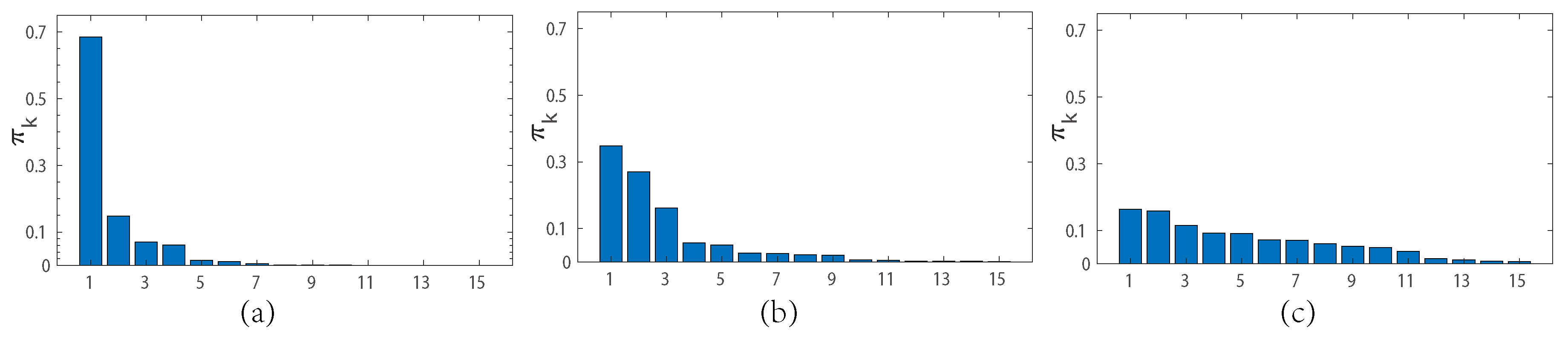
where represents the Dirac Delta function located at . The stick-breaking construction depicts the DP from a different point of view, in which the clustering property of DP is realized by the mixing coefficient . The parameter controls the dispersion level of , and we simulate the stick-breaking process under different in Figure 2. It is easy to see that this stick-breaking process is able to determine the number of Gaussian components of MoG through adjusting the value of .
2.2. Hierarchical Dirichlet Process
The hierarchical Dirichlet process (HDP) [43] is originally proposed as a hierarchical Bayesian model for natural language processing, which provides a flexible framework for sharing mixture components among groups of related data. A two-level HDP is a collection of DPs, which is also drawn from a higher-level DP with base distribution H, i.e.,
where j is an index for the data group. It should be noted that all distributions possess different parameters while sharing the distribution G.
3. HSIs Restoration Model Based on DP-GMM
3.1. Notation Explanation
For convenience of formulating our model, we first introduce some necessary notations to be used in the following sections. We use light lowercase letters, bold lowercase letters and bold uppercase letters to denote scalars, vectors and matrices, respectively. Given a matrix , we use to denote its j-th column vector, to denote its i-th row vector, and to denote the element in its i-th row and j-th column. For probability distributions, represents the multivariate Gaussian distribution with mean vector and covariance matrix , represents the univariate Gaussian distribution with mean and precision , represents the Beta distribution with parameters a and b, represents the Gamma distribution with parameters c and d, and represents the multinomial distribution with parameter .
3.2. Model Formulation
Now, we give the formulations of our proposed model. Let us present the observed HSI data contaminated by noises as , where , h and w are the height and width of the investigated HSI, respectively, and B is the number of bands. By considering a generative model, we can decompose the observed data into
where denotes the noise term and is the expected restorated HSI.
3.2.1. The DP-GMM Model
In this study, we model the noise of each band as a DP-GMM, which is an advanced version of the non-parametric GMM model capable of adaptively rectifying the number of Gaussian components of MoG based on the data [44,45]. The noise complexity of each band can be adjusted by varying the number of components of MoG. What is more, in order to simultaneously encode the correlation among different bands, we associate the corresponding DP-GMM of each band at a higher level and conduct a two-level HDP.
Specifically, we consider the noise located at the i-th row and j-th column of the noise term . Following the idea of [40,46], we can model it as an element-wise Gaussian mixture distribution:
which can be equivalently reformulated as a two-level generative process:
where is a vector of length K, . Then, we place a hierarchical Dirichlet distribution prior on to associate the noise of different bands, i.e.,
Besides, is also generated from its conjugate prior, i.e.,
To allow the model to be flexible, we further assume . Teh et al. [47] proved that the limit of Equations (5)–(7) is the following HDP noise model:
where .
The noise model of Equation (8) is too metaphysical to understand, so we reformulate it equivalently but more explicitly with two coupled latent variables and in a stick-breaking constructive manner, i.e.,
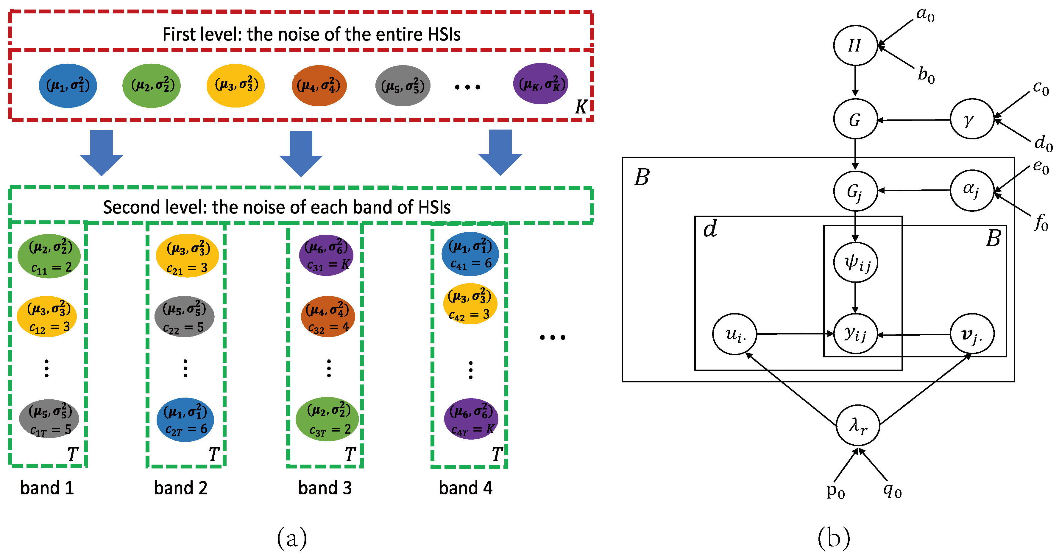
We can explain the hierarchical structure of the noise model (8) using Figure 3a intuitively. In the first level, we attempt to fit the noise of the entire HSI data by a DP-GMM. In the second level, we also fit the noise of each band by a DP-GMM, but each of its components is shared from the first level. This sharing strategy associates the noise of different bands, and the DP-GMM, which allows an MoG to have a limited but unbounded number of Gaussian components, adjusts the noise complexity adaptivity for each band.
Note that we adopt the truncation strategy [48] for the DP-GMMs in the variational inference of Section 4, which means that the number of Gaussian components of DP-GMMs in the first and second levels are fixed as K and T (K and T is large enough, ) as shown in Figure 3a. Based on such a truncation strategy, () denotes the index of the Gaussian component from which is generated in the DP-GMM of band j (), and (, ) denotes the index of the Gaussian component of DP-GMM in the first level, with which the t-th Gaussian component of DP-GMM of band j in the second level is shared ( is marked in Figure 3a).
Finally, the concentration parameters and in Equation (8) mainly affect the number of Gaussian components of the second level MoG in each band and the first level MoG for the entire HSIs dataset, respectively. In order to enhance the adaptability of the model complexity, we can place the Gamma distribution on them [49], i.e.,
In the above formulations, are hyperparameters of prior distributions, all of which can be easily set as small values to make the prior non-informative.
3.2.2. LRMF Model
As the conventional HSI restoration model, we assume that the expected HSI in Equation (3) has a low-rank property. Based on such an assumption, we formulate as the product of two smaller matrices and , i.e.,
where is fixed pre-manually. Furthermore, and can be generated from a multivariate zero-mean Gaussian distribution by the following method:
where denotes the identity matrix. Furthermore, the corresponding conjugate prior on each precision variable is:
3.2.3. The Entire Graphical Model
4. Variational Inference
Directly computing the posterior of Equation (14) under an HDP mixture prior is intractable, and thus approximate inference methods need to be designed. Although the Markov chain Monte Carlo (MCMC) sampling method can provide very accurate approximation to the posterior [50], this method is limited for massive scale data due to its high computational cost and difficulty to detect convergence. As a more efficient and deterministic alternative to MCMC, we adopt a Variational Bayes (VB) method [51] to solve our model in this paper. Given the observed data , maximizing the marginal log-likelihood directly is computationally intractable. VB attempts to seek a lower bound of the log-likelihood and maximize it instead, i.e.,
where denotes the (KL) divergence of two distributions. Assuming , we can obtain the closed-form solution to with other factors fixed through optimizing with respect to , i.e.,
where denotes the expectation over the variable x, and represents the set of with removed. The entire inference can be accomplished by alternatively computing Equation (16) with respect to all the involved variables.
Based on the stick-breaking construction and the truncation strategy [48], we can approximate the posterior distribution of Equation (14) with the following factorized form:
Then we can analytically infer all the factorized distributions involved in Equation (17) as below. The computational details are provided in the Supplementary Material.
Update Noise Component: The parameters involved in the noise components are , , , , . We use the stick-breaking procedure by setting a large enough value of K and T for truncated approximation, and then get the following updating equations on and :
where
As for , based on its conjugate priors, we have
where
Similarly, for , , we have
where
Update the Concentration Parameters: According to the conjugate priors of and in Equation (10), we can obtain the following updating equations:
where
Update the LRMF Components: The parameters involved in the LRMF components are , , . For each row of , using the factorization in Equation (11), we can obtain
with mean and covariance matrix , given by
where . Similarly, for each column of , we have
and the mean and the covariance matrix are calculated by
For parameter , we have
where
Settings of Hyperparameters: We set all the hyperparameters involved in our model in a non-informative manner to minimize their impacts on the inference of the posterior distribution [51]. Specifically, throughout our experiments, we easily set , , , , , , , as . Our proposed method behaves stably throughout all the experiments with this simple initialization choice.
5. Experimental Results
To demonstrate the effectiveness of the proposed DP-GMM model, we perform both synthetic and real HSI data experiments, and evaluate the experimental results quantitatively and visually. In order to comprehensively evaluate the performance of the proposed method, we compared the results with eight popular HSI restoration methods: the traditional image denoising method SVD [52], LRMF-based methods LRMR [20], LRTV [38], WNNM [24] and WSNM [23], tensor-based methods TDL [30] and BM4D [35], and mixture noise based-method NMoG [33]. These methods represent the state-of-the-art for the HSI restoration task. The parameters for these compared methods were manually adjusted according to their default strategies. In addition, to facilitate the numerical calculation and visualization, all the bands of the HSI datasets are normalized into [0,1].
5.1. Simulated Data Experiments
Two HSI datasets were employed in this experiment: Washington DC Mall (http://lesun.weebly.com/hyperspectral-data-set.html) with size and RemoteImage (http://peterwonka.net/Publications/code/LRTC_Package_Ji.zip) with size . Some bands of these two HSI datasets are heavily contaminated by noise and cannot be regarded as clean ground truth, and thus have to be deleted [33,36]. Due to the computer’s memory limitation, we also cropped the subimage of the HSI and finally obtained two synthetic datasets with size and , respectively. These two HSI datasets are considered as clean data in this simulated experiment.
To simulate noisy HSIs, we added six types of noises to the clean HSI datasets to test the performance of all the compared methods. The details of the added noise are listed as follows:
- Case 1: For different bands, the noise intensity was equal in this case. Furthermore, the same zero-mean Gaussian noise with was added to all the bands
- Case 2: Entries in all bands were corrupted by zero-mean Gaussian noise but with different intensity. Furthermore, the standard deviation of Gaussian noise that was added to each band of HSIs was uniformly selected from 0.01 to 0.1.
- Case 3: All the bands were corrupted by Gaussian noise as Case 2. Besides, 40 bands of the DC Mall dataset (20 bands of the RemoteImage dataset) were randomly chosen to add deadlines, and the number of deadlines in each band is from 5 to 15 with width 1 or 2.
- Case 4: All the bands were contaminated by Gaussian noise as Case 2. Besides, 40 bands of the DC Mall dataset (20 bands of the RemoteImage) were randomly selected to add stripes, and the number of stripes is from 15 to 40 with width 1 or 2.
- Case 5: All the bands were corrupted by Gaussian noise as Case 2. In addition, different percentages of impulse noises which were uniformly selected from 0 to 0.15 were added to each band.
- Case 6: Each band was contaminated by Gaussian and impulse noise as Case 5. Besides, 20 bands of the DC Mall dataset (10 bands of the RemoteImage dataset) were randomly selected to add deadlines as Case 3, and another 20 bands of the DC Mall dataset (10 bands of the RemoteImage dataset) were randomly selected to add stripes as Case 4.
To fairly compare the overall performance of different methods, we set the rank of the expected HSIs as 7 in the DC Mall and RemoteImage dataset for all the compared methods. Furthermore, three measurements—the mean peak signal-to-noise ratio (MPSNR), mean structural similarity index (MSSIM) [53] and Erreur Relative Globale Adimensionnelle de Synthèse (ERGAS) [54]—are utilized to evaluate the restoration quality:
where and denote the PSNR and SSIM values for the i-th band, and and denote the i-th band of the reference image and the restorated image, respectively.
Table 1 and Table 2 present the restoration results by all the compared methods in terms of the aforementioned three measurements. The best results for each quality measurement are highlighted in bold. It is clear that our proposed method provides the highest values in both MPSNR and MSSIM, and lowest ERGAS in most of the cases, which validates the superiority of the proposed method over the other methods. For Case 1 with the simple independent and identically distributed (i.i.d.) Gaussian noise, most of the methods have comparable performance, which confirms the effectiveness of these methods to some extent, especially for TDL. When the noise becomes more complex, e.g., the intensity of noise varies by bands, more stripes, more deadlines and more impulse noises are added, the advantages of our proposed method become more evident from Case 2 to Case 6. This advantage substantiates the robustness of our proposed method against complex noise, owing to its adaptability to distinguish noise complexities in different HSI bands in our model.
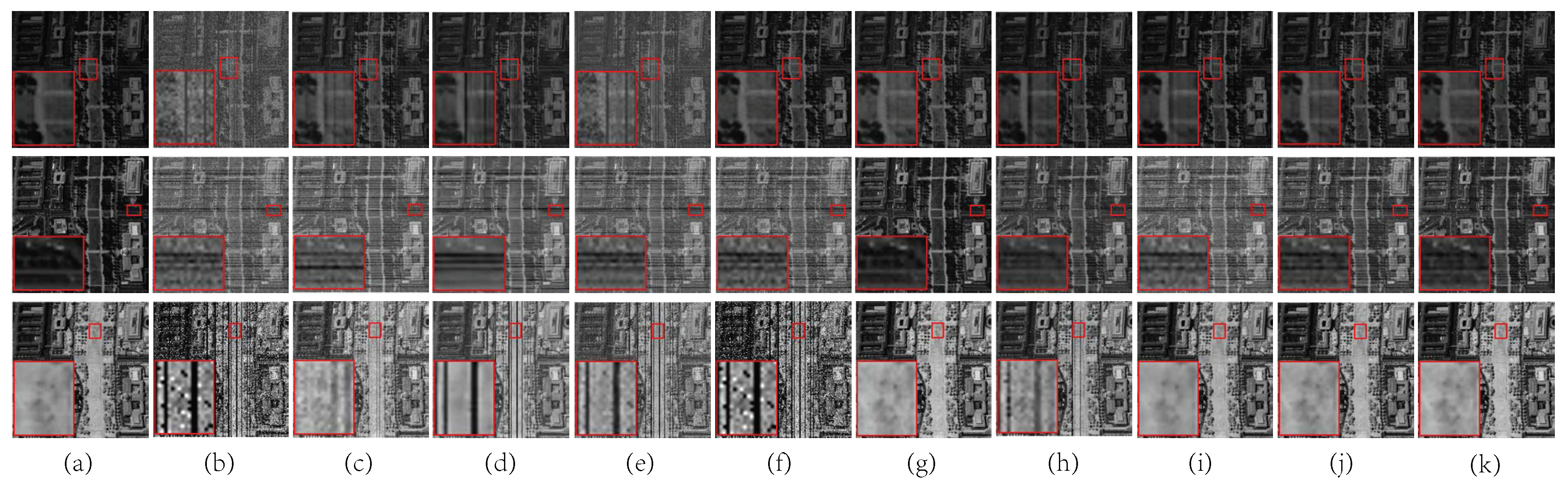
Figure 4 and Figure 5 present some typical bands of the DC Mall and RemoteImage HSI dataset before and after restoration under Case 3, Case 4 and Case 6, respectively. By comparing the restoration results, it can be clearly seen that DP-GMM performs best, effectively removing all types of noise while preserving more detailed information. In Case 3, the restored HSIs of almost all of the compared methods contain some evident deadlines. Similarly, some stripes still exist in the restoration results of most of the compared methods in Case 4. Under the mixture noise of Case 6, LRTV, NMoG and DP-GMM all have relatively better results than the other methods. In conclusion, our proposed method can have stable and better performance in all cases, which verifies the effectiveness of the proposed method with better capability in fitting a much wider range of noises than current methods.
In order to further compare the performance of all the restoration methods, we also show the spectral signatures of some pixels before and after restoration; for example, Figure 6 shows the spectrum of pixels (55, 110) and (110, 184) for the DC Mall HSI dataset under Case 6, and Figure 7 shows similar results for the RemoteImage HSI dataset. It is easy to see that our proposed method provides the best spectral signature among all of the compared methods, which is closest to the original one. Besides, the NMoG method, which adopts non-i.i.d. MoG to model the noises of HSIs, also has comparable performance. These advantages of DP-GMM and NMoG indicate the necessity of giving more consideration to the complex noise structure of HSIs.
5.2. Real Data Experiments
In this section, two real-world test HSI datasets are used in our experiments: the Hyperspectral Digital Imagery Collection Experiment (HYDICE) Urban (http://lesun.weebly.com/hyperspectral-data-set.html) dataset and the Army Geospatial Center (AGC) Terrain (https://www.agc.army.mil) dataset.
HYDICE Urban Dataset: The original image is in size, and we feed the entire dataset into the denoising algorithms directly. Some bands of Urban are seriously polluted by the atmosphere, water absorption and other unknown noises, such as bands 104–108, 139–151 and 206–210. Additionally, some other bands are contaminated by stripes, deadlines and Gaussian noise, such as bands 1–2, 76 and 198. In this first real data experiment, the rank is set as 7 for all the competing methods.
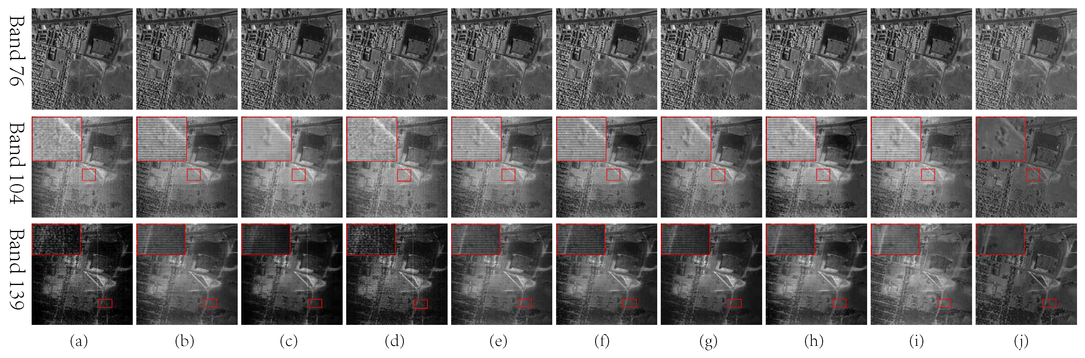
Figure 8 shows bands 76 (top), 104 (middle) and 139 (bottom) of the restored HSIs of the Urban dataset, and these three bands are typically polluted to varying degrees by different types of noise as analyzed in Figure 1a. Band 76 is relatively clean with several deadlines, and most of the competing methods can remove these deadlines except TDL and BM4D. As for bands 104 and 139, however, some stripes still exist in the restored images for almost all the competing methods. This is because these bands are heavily corrupted and can provide little useful information, and these methods lack noise adaptivity to deal with these complex cases. In contrast, our proposed DP-GMM method is able to completely suppress the stripes and effectively preserves the detailed information. What is more, the images restored by our proposed method are smoother than those restored by other compared methods. These visual results show that our proposed DP-GMM method can remove more complicated noise embedded in HSIs than other competing methods.
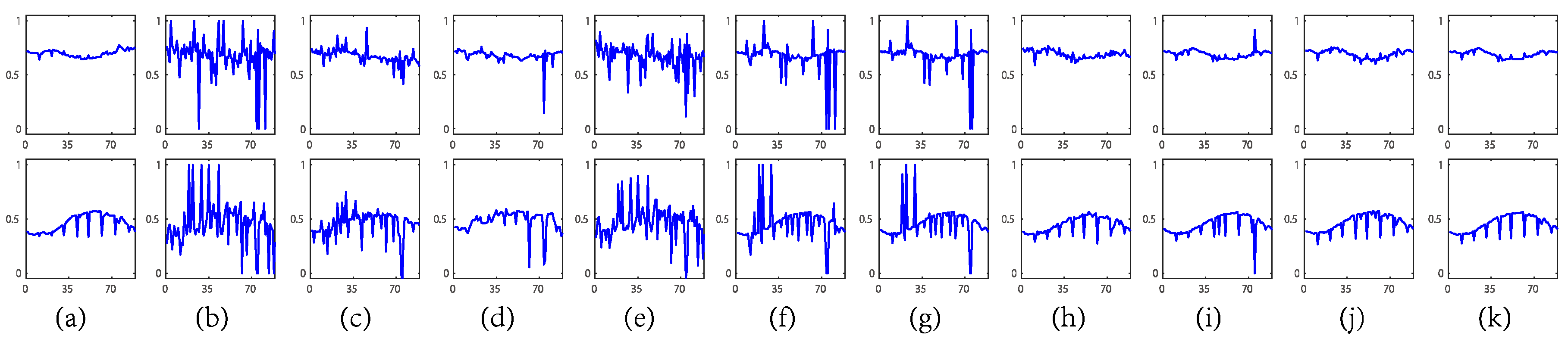
Figure 9 shows the vertical mean profiles of bands 76, 104 and 139, which is a quantitative comparison of the restorated results shown in Figure 8. The horizontal axis in Figure 8 represents the column number, and the vertical axis represents the mean digital number value of each column. Band 76 is almost noise-free with only one deadline. There is thus no visible change between the mean profiles before and after the restoration. When the noise becomes more complicated, the curves fluctuate rapidly in the original images for bands 104 and 139. After the restoration processing, the fluctuations are more or less suppressed. Obviously, the DP-GMM methods perform best and obtain the flattest curve without fluctuations. These results are in accordance with the visual results of Figure 8.
AGC Terrain Dataset: The second real data experiment employed the Terrain dataset as the test dataset, and it has pixels and 210 bands. The full Terrain image is mainly corrupted by deadlines, atmosphere, water absorption and others, especially the bands 104–109, 138–152 and 204–210. We also set the rank as 7 in this experiment for all the methods.
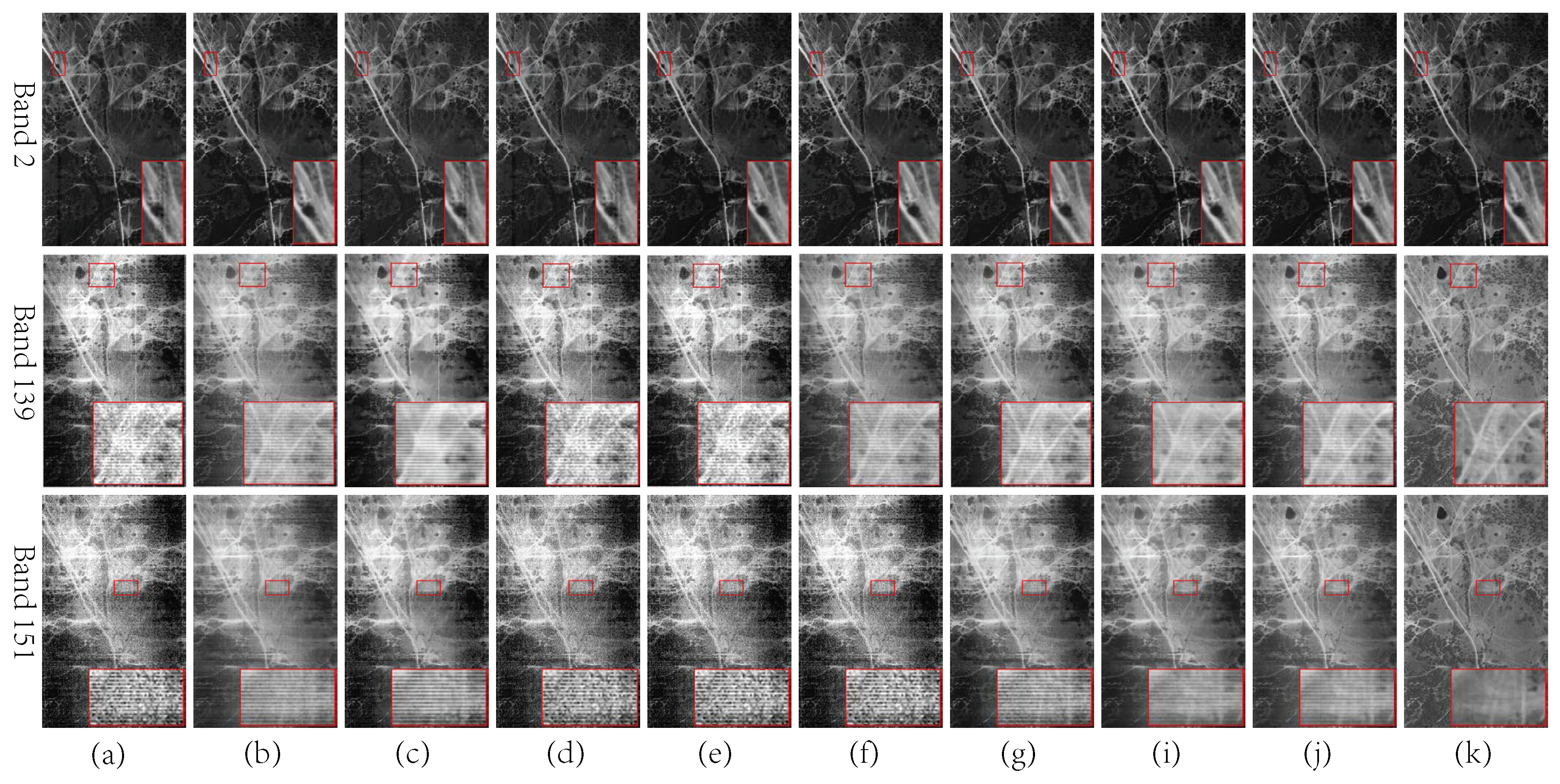
We selected three typical bands 2, 139 and 151 to display the performance of all the compared methods in Figure 10. These three bands exhibit evident noise distinctness, as shown in Figure 1b, both in terms of distribution types and corruption extent. In band 2, there are some deadlines clustered together, as shown in the amplified area, and SVD, BM4D, WNNM, WSNM, LRMR, LRTV and our proposed DP-GMM can all remove these deadlines completely. As for bands 139 and 151, which contain many stripes and other mixed noise, it is easy to see that the DP-GMM removes more noise, especially stripes, compared with the other methods, owing to its noise adaptivity for different bands. These visual results show that our proposed DP-GMM method is more robust when dealing with the complicated real noise of HSI data.
Figure 11 shows the vertical mean profiles comparison before and after restoration for each competing method, corresponding to the visualization of Figure 10. The horizontal axis in this figure represents the column number, and the corresponding vertical axis represents the mean digital number value of each column. The curves obtained by different methods in band 2 appear to be slightly smoother to different degrees, as compared with that of the original images. However, as for bands 139 and 151, due to the interference of the mixed noise, especially stripes and deadlines, there are sharp fluctuations in the curve for the original images. After the restoration, the fluctuations are suppressed by all of the competing methods to some extent. Obviously, the curves obtained by our proposed method are smoother than others, which indicates the better restoration results of DP-GMM. These quantitative results are also in accordance with the visual results of Figure 10.
6. Conclusions
We have proposed a new HSI restoration method by constructing the noise model as a DP-GMM under the Bayesian framework. Most of the current methods do not give much consideration to the variation of the noise complexity among the different bands of the natural HSI. In contrast, our method uses a hierarchical structure to fit the noise so that the noise of different HSI bands can be flexibly encoded by MoGs with different mixture component numbers. The noise distinctness among HSI bands can thus be faithfully reflected in the model, potentially making it more robust in real HSI scenarios. In order to validate the effectiveness of the proposed methods, we conducted a series of experiments on synthetic and real HSI datasets. For the synthetic HSI datasets, our proposed method performed better than all the competing methods in terms of MPSNR, MSSIM and ERGAS. Specifically, in terms of the MPSNR, our method is on average over 1 dB higher than the current state-of-the-art methods: LRTV and NMoG. For the real HSI dataset, our proposed method can remove almost all of the noises, and obtain better visual restoration results compared with other methods, especially for the heavily contaminated bands.
Supplementary Materials
The following are available online at https://www.mdpi.com/2072-4292/10/10/1631/s1.
Author Contributions
All authors designed the study and discussed the basic structure of the manuscript. Z.Y. carried out the experiments and finished the original version of this paper. D.M. administrated the project. Y.S. validated the results. Z.Y. and Q.Z. designed the experiments. D.M. and Q.Z. reviewed and edited the paper.
Funding
This research was supported by National Key R&D Program of China (2018YFB1004300), the China NSFC projects under contracts 61661166011, 61603292, 11690011, 61721002.
Conflicts of Interest
The authors declare no conflict of interest.
References
- Goetz, A.F. Three decades of hyperspectral remote sensing of the Earth: A personal view. Remote Sens. Environ. 2009, 113, S5–S16. [Google Scholar] [CrossRef]
- Willett, R.M.; Duarte, M.F.; Davenport, M.A.; Baraniuk, R.G. Sparsity and structure in hyperspectral imaging: Sensing, reconstruction, and target detection. IEEE Signal Process. Mag. 2014, 31, 116–126. [Google Scholar] [CrossRef]
- Liu, X.; Bourennane, S.; Fossati, C. Nonwhite noise reduction in hyperspectral images. IEEE Geosci. Remote Sens. Lett. 2012, 9, 368–372. [Google Scholar] [CrossRef]
- Bioucas-Dias, J.M.; Plaza, A.; Dobigeon, N.; Parente, M.; Du, Q.; Gader, P.; Chanussot, J. Hyperspectral unmixing overview: Geometrical, statistical, and sparse regression-based approaches. IEEE J. Sel. Top. Appl. Earth Obs. Remote Sens. 2012, 5, 354–379. [Google Scholar] [CrossRef]
- Camps-Valls, G.; Bruzzone, L. Kernel-based methods for hyperspectral image classification. IEEE Trans. Geosci. Remote Sens. 2005, 43, 1351–1362. [Google Scholar] [CrossRef] [Green Version]
- Elad, M.; Aharon, M. Image denoising via sparse and redundant representations over learned dictionaries. IEEE Trans. Image Process. 2006, 15, 3736–3745. [Google Scholar] [CrossRef] [PubMed]
- Dabov, K.; Foi, A.; Katkovnik, V.; Egiazarian, K. Image denoising by sparse 3-D transform-domain collaborative filtering. IEEE Trans. Image Process. 2007, 16, 2080–2095. [Google Scholar] [CrossRef] [PubMed]
- Mairal, J.; Bach, F.; Ponce, J.; Sapiro, G.; Zisserman, A. Non-local sparse models for image restoration. In Proceedings of the 2009 IEEE 12th International Conference on Computer Vision, Kyoto, Japan, 29 September–2 October 2009; pp. 2272–2279. [Google Scholar]
- Liu, L.; Chen, L.; Chen, C.P.; Tang, Y.Y.; Pun, C.M. Weighted joint sparse representation for removing mixed noise in image. IEEE Trans. Cybern. 2017, 47, 600–611. [Google Scholar] [CrossRef] [PubMed]
- Lerga, J.; Sucic, V.; Vrankić, M. Separable image denoising based on the relative intersection of confidence intervals rule. Informatica 2011, 22, 383–394. [Google Scholar]
- Lerga, J.; Sucic, V.; Sersic, D. Performance analysis of the LPA-RICI denoising method. In Proceedings of the 6th International Symposium on Image and Signal Processing and Analysis, Salzburg, Austria, 16–18 September 2009; pp. 28–33. [Google Scholar]
- Mandic, I.; Peic, H.; Lerga, J.; Stajduhar, I. Denoising of X-ray images using the adaptive algorithm based on the LPA-RICI algorithm. J. Imaging 2018, 4, 34. [Google Scholar] [CrossRef]
- Othman, H.; Qian, S.E. Noise reduction of hyperspectral imagery using hybrid spatial-spectral derivative-domain wavelet shrinkage. IEEE Trans. Geosci. Remote Sens. 2006, 44, 397–408. [Google Scholar] [CrossRef]
- Chen, G.; Qian, S.E. Simultaneous dimensionality reduction and denoising of hyperspectral imagery using bivariate wavelet shrinking and principal component analysis. Can. J. Remote Sens. 2008, 34, 447–454. [Google Scholar] [CrossRef]
- Chen, S.L.; Hu, X.Y.; Peng, S.L. Hyperspectral imagery denoising using a spatial-spectral domain mixing prior. J. Comput. Sci. Technol. 2012, 27, 851–861. [Google Scholar] [CrossRef]
- Yuan, Q.; Zhang, L.; Shen, H. Hyperspectral image denoising employing a spectral-spatial adaptive total variation model. IEEE Trans. Geosci. Remote Sens. 2012, 50, 3660–3677. [Google Scholar] [CrossRef]
- Qian, Y.; Ye, M. Hyperspectral imagery restoration using nonlocal spectral-spatial structured sparse representation with noise estimation. IEEE J. Sel. Top. Appl. Earth Obs. Remote Sens. 2013, 6, 499–515. [Google Scholar] [CrossRef]
- Wang, Y.; Niu, R.; Yu, X. Anisotropic diffusion for hyperspectral imagery enhancement. IEEE Sens. J. 2010, 10, 469–477. [Google Scholar] [CrossRef]
- Zhong, P.; Wang, R. Multiple-spectral-band CRFs for denoising junk bands of hyperspectral imagery. IEEE Trans. Geosci. Remote Sens. 2013, 51, 2260–2275. [Google Scholar] [CrossRef]
- He, W.; Zhang, H.; Zhang, L.; Shen, H. Hyperspectral image denoising via noise-adjusted iterative low-rank matrix approximation. IEEE J. Sel. Top. Appl. Earth Obs. Remote Sens. 2015, 8, 3050–3061. [Google Scholar] [CrossRef]
- Candès, E.J.; Li, X.; Ma, Y.; Wright, J. Robust principal component analysis? J. ACM (JACM) 2011, 58, 11. [Google Scholar] [CrossRef]
- Wu, Z.; Wang, Q.; Wu, Z.; Shen, Y. Total variation-regularized weighted nuclear norm minimization for hyperspectral image mixed denoising. J. Electron. Imaging 2016, 25, 013037. [Google Scholar] [CrossRef]
- Xie, Y.; Qu, Y.; Tao, D.; Wu, W.; Yuan, Q.; Zhang, W. Hyperspectral Image Restoration via Iteratively Regularized Weighted Schatten p-Norm Minimization. IEEE Trans. Geosci. Remote Sens. 2016, 54, 4642–4659. [Google Scholar] [CrossRef]
- Gu, S.; Zhang, L.; Zuo, W.; Feng, X. Weighted nuclear norm minimization with application to image denoising. In Proceedings of the IEEE Conference on Computer Vision and Pattern Recognition, Columbus, OH, USA, 23–28 June 2014; pp. 2862–2869. [Google Scholar]
- Peng, Y.; Suo, J.; Dai, Q.; Xu, W. Reweighted low-rank matrix recovery and its application in image restoration. IEEE Trans. Cybern. 2014, 44, 2418–2430. [Google Scholar] [CrossRef] [PubMed]
- Wang, M.; Yu, J.; Xue, J.H.; Sun, W. Denoising of hyperspectral images using group low-rank representation. IEEE J. Sel. Top. Appl. Earth Obs. Remote Sens. 2016, 9, 4420–4427. [Google Scholar] [CrossRef]
- Xie, Q.; Zhao, Q.; Meng, D.; Xu, Z.; Gu, S.; Zuo, W.; Zhang, L. Multispectral images denoising by intrinsic tensor sparsity regularization. In Proceedings of the IEEE Conference on Computer Vision and Pattern Recognition, Las Vegas, NV, USA, 27–30 June 2016; pp. 1692–1700. [Google Scholar]
- Karami, A.; Yazdi, M.; Asli, A.Z. Noise reduction of hyperspectral images using kernel non-negative tucker decomposition. IEEE J. Sel. Top. Signal Process. 2011, 5, 487–493. [Google Scholar] [CrossRef]
- Liu, X.; Bourennane, S.; Fossati, C. Denoising of hyperspectral images using the PARAFAC model and statistical performance analysis. IEEE Trans. Geosci. Remote Sens. 2012, 50, 3717–3724. [Google Scholar] [CrossRef]
- Peng, Y.; Meng, D.; Xu, Z.; Gao, C.; Yang, Y.; Zhang, B. Decomposable nonlocal tensor dictionary learning for multispectral image denoising. In Proceedings of the IEEE Conference on Computer Vision and Pattern Recognition, Columbus, OH, USA, 23–28 June 2014; pp. 2949–2956. [Google Scholar]
- Wang, Y.; Peng, J.; Zhao, Q.; Leung, Y.; Zhao, X.L.; Meng, D. Hyperspectral image restoration via total variation regularized low-rank tensor decomposition. IEEE J. Sel. Top. Appl. Earth Obs. Remote Sens. 2018, 11, 1227–1243. [Google Scholar] [CrossRef]
- Letexier, D.; Bourennane, S. Noise removal from hyperspectral images by multidimensional filtering. IEEE Trans. Geosci. Remote Sens. 2008, 46, 2061–2069. [Google Scholar] [CrossRef]
- Chen, G.; Qian, S.E. Denoising of hyperspectral imagery using principal component analysis and wavelet shrinkage. IEEE Trans. Geosci. Remote Sens. 2011, 49, 973–980. [Google Scholar] [CrossRef]
- Chen, G.; Zhu, W.P. Signal denoising using neighbouring dual-tree complex wavelet coefficients. IET Signal Process. 2012, 6, 143–147. [Google Scholar] [CrossRef]
- Maggioni, M.; Katkovnik, V.; Egiazarian, K.; Foi, A. Nonlocal transform-domain filter for volumetric data denoising and reconstruction. IEEE Trans. Image Process. 2013, 22, 119–133. [Google Scholar] [CrossRef] [PubMed]
- Zhang, H.; He, W.; Zhang, L.; Shen, H.; Yuan, Q. Hyperspectral image restoration using low-rank matrix recovery. IEEE Trans. Geosci. Remote Sens. 2014, 52, 4729–4743. [Google Scholar] [CrossRef]
- Chen, X.; Han, Z.; Wang, Y.; Zhao, Q.; Meng, D.; Lin, L.; Tang, Y. A general model for robust tensor factorization with unknown noise. arXiv, 2017; arXiv:1705.06755. [Google Scholar]
- He, W.; Zhang, H.; Zhang, L.; Shen, H. Total-variation-regularized low-rank matrix factorization for hyperspectral image restoration. IEEE Trans. Geosci. Remote Sens. 2016, 54, 178–188. [Google Scholar] [CrossRef]
- Cao, X.; Zhao, Q.; Meng, D.; Chen, Y.; Xu, Z. Robust low-rank matrix factorization under general mixture noise distributions. IEEE Trans. Image Process. 2016, 25, 4677–4690. [Google Scholar] [CrossRef] [PubMed]
- Chen, Y.; Cao, X.; Zhao, Q.; Meng, D.; Xu, Z. Denoising hyperspectral image with non-iid noise structure. IEEE Trans. Cybern. 2018, 48, 1054–1066. [Google Scholar] [CrossRef] [PubMed]
- Ferguson, T.S. A Bayesian analysis of some nonparametric problems. Ann. Stat. 209–230. [CrossRef]
- Sethuraman, J. A constructive definition of Dirichlet priors. Stat. Sin. 639–650.
- Teh, Y.W.; Jordan, M.I.; Beal, M.J.; Blei, D.M. Sharing clusters among related groups: Hierarchical Dirichlet processes. In Advances in Neural Information Processing Systems 17; MIT Press: Cambridge, MA, USA; Lodon, UK, 2005; pp. 1385–1392. [Google Scholar]
- Rasmussen, C.E. The infinite Gaussian mixture model. In Advances in Neural Information Processing Systems 12; MIT Press: Cambridge, MA, USA; Lodon, UK, 2000; pp. 554–560. [Google Scholar]
- Chen, P.; Wang, N.; Zhang, N.L.; Yeung, D.Y. Bayesian adaptive matrix factorization with automatic model selection. In Proceedings of the IEEE Conference on Computer Vision and Pattern Recognition, Boston, MA, USA, 7–12 June 2015; pp. 1284–1292. [Google Scholar]
- Meng, D.; De La Torre, F. Robust matrix factorization with unknown noise. In Proceedings of the IEEE International Conference on Computer Vision, Sydney, Australia, 1–8 December 2013; pp. 1337–1344. [Google Scholar]
- Teh, Y.W.; Jordan, M.I.; Beal, M.J.; Blei, D.M. Hierarchical Dirichlet Processes. Publ. Am. Stat. Assoc. 2006, 101, 1566–1581. [Google Scholar] [CrossRef] [Green Version]
- Blei, D.M.; Jordan, M.I. Variational inference for Dirichlet process mixtures. Bayesian Anal. 2006, 1, 121–143. [Google Scholar] [CrossRef]
- MacEachern, S.N.; Müller, P. Estimating mixture of Dirichlet process models. J. Comput. Graph. Stat. 1998, 7, 223–238. [Google Scholar]
- Neal, R.M. Markov chain sampling methods for Dirichlet process mixture models. J. Comput. Graph. Stat. 2000, 9, 249–265. [Google Scholar]
- Bishop, C.M. Pattern Recognition and Machine Learning; Springer: Berlin/Heidelberg, Germany, 2006; pp. 140–155. [Google Scholar]
- Haardt, M.; Strobach, P. Method for High-Resolution Spectral Analysis in Multi Channel Observations Using a Singular Valve Decomposition (SVD) Matrix Technique. US Patent 5,560,367, 1996. [Google Scholar]
- Wang, Z.; Bovik, A.C.; Sheikh, H.R.; Simoncelli, E.P. Image quality assessment: from error visibility to structural similarity. IEEE Trans. Image Process. 2004, 13, 600–612. [Google Scholar] [CrossRef] [PubMed]
- Wald, L. Data Fusion: Definitions and Architectures: Fusion of Images Of Different Spatial Resolutions; Presses des MINES: Paris, France, 2002. [Google Scholar]
Figure 1.
The distinctness of noises among different bands of hyperspectral images (HSIs). (a) Bands 76, 104 and 139 of the Urban HSI dataset; (b) Bands 2, 139 and 151 of the Terrain HSI dataset. (a1) and (b1): Original images, (a2) and (b2): restored images, (a3) and (b3): noises extracted by our proposed method, (a4) and (b4): histogram of noises in the same scale.
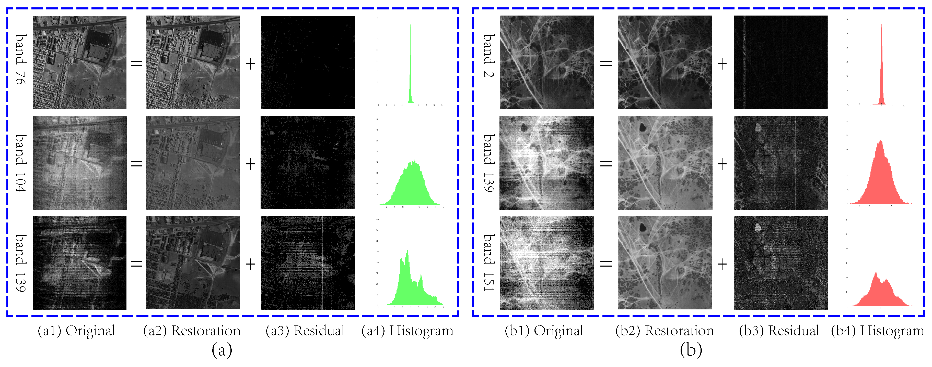
Figure 2.
Stick breaking process under different concentration parameters . (a) ; (b) ; (c) .

Figure 3.
(a): Illustration of the hierarchical DP-GMM model for HSI restoration. The ellipses with different colors denote the Gaussian component with parameters (, ). The green dotted rectangles, representing the Gaussian compounds of each band, share Gaussian components from a top-level MoG in the red dotted rectangle. The number of Gaussian components of MoG at the two levels are dynamically adjusted during the HSI restoration until it converges. (b): The entire graphic model of DP-GMM.

Figure 4.
From top to bottom: restoration results of band 118, 20 and 66 of the DCmall HSI dataset under case 3, case 4 and case 6, respectively. (a) Original HSI; (b) Noisy HSI; (c) SVD; (d) BM4D; (e) TDL; (f) WNNM; (g) WSNM; (h) LRMR; (i) LRTV; (j) NMoG; (k) DP-GMM.
Figure 4.
From top to bottom: restoration results of band 118, 20 and 66 of the DCmall HSI dataset under case 3, case 4 and case 6, respectively. (a) Original HSI; (b) Noisy HSI; (c) SVD; (d) BM4D; (e) TDL; (f) WNNM; (g) WSNM; (h) LRMR; (i) LRTV; (j) NMoG; (k) DP-GMM.

Figure 5.
From top to bottom: restoration results of band 49, 11 and 74 of the RemoteImage HSI dataset under Case 3, Case 4 and Case 6, respectively. (a) Original HSI; (b) Noisy HSI; (c) SVD; (d) BM4D; (e) TDL; (f) WNNM; (g) WSNM; (h) LRMR; (i) LRTV; (j) NMoG; (k) DP-GMM.
Figure 5.
From top to bottom: restoration results of band 49, 11 and 74 of the RemoteImage HSI dataset under Case 3, Case 4 and Case 6, respectively. (a) Original HSI; (b) Noisy HSI; (c) SVD; (d) BM4D; (e) TDL; (f) WNNM; (g) WSNM; (h) LRMR; (i) LRTV; (j) NMoG; (k) DP-GMM.

Figure 6.
From top to bottom: Spectrum of pixels (55,110) and (110, 184) for the DC Mall HSI dataset. From left to right: (a) Original HSI; (b) Noisy HSI; (c) SVD; (d) BM4D; (e) TDL; (f) WNNM; (g) WSNM; (h) LRMR; (i) LRTV; (j) NMoG; (k) DP-GMM.
Figure 6.
From top to bottom: Spectrum of pixels (55,110) and (110, 184) for the DC Mall HSI dataset. From left to right: (a) Original HSI; (b) Noisy HSI; (c) SVD; (d) BM4D; (e) TDL; (f) WNNM; (g) WSNM; (h) LRMR; (i) LRTV; (j) NMoG; (k) DP-GMM.

Figure 7.
From top to bottom: Spectrum of pixels (78,61) and (137, 41) for the RemoteImage HSI dataset. From left to right: (a) Original HSI; (b) Noisy HSI; (c) SVD; (d) BM4D; (e) TDL; (f) WNNM; (g) WSNM; (h) LRMR; (i) LRTV; (j) NMoG; (k) DP-GMM.
Figure 7.
From top to bottom: Spectrum of pixels (78,61) and (137, 41) for the RemoteImage HSI dataset. From left to right: (a) Original HSI; (b) Noisy HSI; (c) SVD; (d) BM4D; (e) TDL; (f) WNNM; (g) WSNM; (h) LRMR; (i) LRTV; (j) NMoG; (k) DP-GMM.

Figure 8.
From top to bottom: restoration results of bands 76, 104 and 139 of the real Urban HSI dataset. (a) Original HSI; (b) SVD; (c) BM4D; (d) TDL; (e) WNNM; (f) WSNM; (g) LRMR; (h) LRTV; (i) NMoG; (j) DP-GMM.
Figure 8.
From top to bottom: restoration results of bands 76, 104 and 139 of the real Urban HSI dataset. (a) Original HSI; (b) SVD; (c) BM4D; (d) TDL; (e) WNNM; (f) WSNM; (g) LRMR; (h) LRTV; (i) NMoG; (j) DP-GMM.

Figure 9.
Vertical mean profiles of some typical bands of the Urban HSI dataset. From top to bottom: band 76 (top), band 104 (middle) and band 139 (down). From left to right: (a) Original HSI; (b) SVD; (c) BM4D; (d) TDL; (e) WNNM; (f) WSNM; (g) LRMR; (h) LRTV; (i) NMoG; (j) DP-GMM.
Figure 9.
Vertical mean profiles of some typical bands of the Urban HSI dataset. From top to bottom: band 76 (top), band 104 (middle) and band 139 (down). From left to right: (a) Original HSI; (b) SVD; (c) BM4D; (d) TDL; (e) WNNM; (f) WSNM; (g) LRMR; (h) LRTV; (i) NMoG; (j) DP-GMM.

Figure 10.
From top to bottom: restoration results of bands 2, 139 and 151 of the real Terrain HSI dataset. (a) Original HSI; (b) SVD; (c) BM4D; (d) TDL; (e) WNNM; (f) WSNM; (g) LRMR; (h) LRTV; (i) NMoG; (j) DP-GMM.
Figure 10.
From top to bottom: restoration results of bands 2, 139 and 151 of the real Terrain HSI dataset. (a) Original HSI; (b) SVD; (c) BM4D; (d) TDL; (e) WNNM; (f) WSNM; (g) LRMR; (h) LRTV; (i) NMoG; (j) DP-GMM.

Figure 11.
Vertical mean profiles of some typical bands in the Terrain HSI dataset. From top to bottom: band 2 (top), band 139 (middle) and band 151 (down). From left to right: (a) Original HSI; (b) SVD; (c) BM4D; (d) TDL; (e) WNNM; (f) WSNM; (g) LRMR; (h) LRTV; (i) NMoG; (j) DP-GMM.
Figure 11.
Vertical mean profiles of some typical bands in the Terrain HSI dataset. From top to bottom: band 2 (top), band 139 (middle) and band 151 (down). From left to right: (a) Original HSI; (b) SVD; (c) BM4D; (d) TDL; (e) WNNM; (f) WSNM; (g) LRMR; (h) LRTV; (i) NMoG; (j) DP-GMM.


Table 1.
Quantitative Evaluation of different methods on the simulated DC Mall dataset in different cases of noise.
Table 1.
Quantitative Evaluation of different methods on the simulated DC Mall dataset in different cases of noise.
| Noise Case | Evaluation Index | Noise | SVD | BM4D | TDL | WNNM | WSNM | LRMR | LRTV | NMoG | DP-GMM |
|---|---|---|---|---|---|---|---|---|---|---|---|
| Case 1 | MPSNR (dB) | 26.02 | 38.96 | 36.66 | 40.23 | 36.98 | 36.98 | 38.79 | 38.45 | 39.05 | 39.60 |
| MSSIM | 0.7627 | 0.9833 | 0.9728 | 0.9888 | 0.9806 | 0.9801 | 0.9848 | 0.9836 | 0.9865 | 0.9875 | |
| ERGAS | 187.97 | 41.37 | 53.24 | 35.34 | 52.74 | 52.74 | 41.98 | 43.27 | 42.19 | 38.22 | |
| Case 2 | MPSNR (dB) | 23.37 | 35.79 | 34.25 | 26.99 | 36.38 | 36.28 | 36.38 | 36.88 | 37.70 | 38.59 |
| MSSIM | 0.6527 | 0.9600 | 0.9535 | 0.7904 | 0.9750 | 0.9732 | 0.9733 | 0.9739 | 0.9818 | 0.9842 | |
| ERGAS | 280.83 | 67.75 | 70.75 | 191.56 | 55.74 | 56.23 | 55.93 | 59.94 | 49.99 | 43.01 | |
| Case 3 | MPSNR (dB) | 22.51 | 33.90 | 31.67 | 25.12 | 35.99 | 35.34 | 34.45 | 35.96 | 36.99 | 37.99 |
| MSSIM | 0.6317 | 0.9486 | 0.9275 | 0.7465 | 0.9730 | 0.9632 | 0.9619 | 0.9695 | 0.9767 | 0.9827 | |
| ERGAS | 308.89 | 102.41 | 128.78 | 240.34 | 59.22 | 81.04 | 84.31 | 76.22 | 65.47 | 47.72 | |
| Case 4 | MPSNR (dB) | 22.50 | 33.80 | 31.56 | 24.66 | 34.95 | 35.26 | 34.64 | 35.77 | 37.09 | 37.55 |
| MSSIM | 0.6211 | 0.9280 | 0.9010 | 0.7035 | 0.9547 | 0.9690 | 0.9540 | 0.9642 | 0.9753 | 0.9790 | |
| ERGAS | 341.01 | 133.14 | 163.27 | 288.97 | 122.49 | 67.43 | 86.43 | 85.27 | 61.36 | 56.19 | |
| Case 5 | MPSNR (dB) | 16.47 | 27.17 | 25.12 | 21.80 | 34.33 | 34.45 | 35.07 | 36.28 | 36.15 | 37.61 |
| MSSIM | 0.4122 | 0.8299 | 0.7339 | 0.5907 | 0.9263 | 0.9716 | 0.9644 | 0.9686 | 0.9688 | 0.9795 | |
| ERGAS | 601.66 | 206.72 | 225.50 | 319.36 | 183.85 | 72.97 | 64.44 | 78.02 | 126.97 | 48.80 | |
| Case 6 | MPSNR (dB) | 16.07 | 26.86 | 24.54 | 20.59 | 33.04 | 33.79 | 33.76 | 34.60 | 35.88 | 36.98 |
| MSSIM | 0.3946 | 0.8202 | 0.7154 | 0.5412 | 0.8975 | 0.9616 | 0.9544 | 0.9599 | 0.9675 | 0.9782 | |
| ERGAS | 625.80 | 209.85 | 240.57 | 368.62 | 240.41 | 104.08 | 83.47 | 112.62 | 469.93 | 54.68 |
Table 2.
Quantitative Evaluation of different methods on the simulated RemoteImage dateset in different cases of noise.
Table 2.
Quantitative Evaluation of different methods on the simulated RemoteImage dateset in different cases of noise.
| Noise Case | Evaluation Index | Noise | SVD | BM4D | TDL | WNNM | WSNM | LRMR | LRTV | NMoG | DP-GMM |
|---|---|---|---|---|---|---|---|---|---|---|---|
| Case 1 | MPSNR (dB) | 26.02 | 37.02 | 34.50 | 37.97 | 34.61 | 35.58 | 37.04 | 36.22 | 36.83 | 37.37 |
| MSSIM | 0.6954 | 0.9655 | 0.9267 | 0.9705 | 0.9570 | 0.9575 | 0.9679 | 0.9588 | 0.9700 | 0.9700 | |
| ERGAS | 124.05 | 37.17 | 50.33 | 33.01 | 50.06 | 43.66 | 36.44 | 40.02 | 38.40 | 35.76 | |
| Case 2 | MPSNR (dB) | 23.25 | 33.85 | 32.12 | 27.65 | 34.18 | 33.02 | 34.67 | 34.72 | 35.56 | 35.79 |
| MSSIM | 0.5554 | 0.9272 | 0.8785 | 0.7636 | 0.9399 | 0.8956 | 0.9464 | 0.9406 | 0.9610 | 0.9605 | |
| ERGAS | 186.22 | 54.26 | 64.95 | 112.77 | 50.80 | 82.17 | 47.62 | 47.44 | 44.30 | 42.69 | |
| Case 3 | MPSNR (dB) | 21.86 | 30.67 | 28.78 | 24.63 | 33.56 | 30.52 | 32.46 | 33.86 | 34.40 | 35.93 |
| MSSIM | 0.5233 | 0.8764 | 0.8102 | 0.6693 | 0.9280 | 0.8246 | 0.9220 | 0.9314 | 0.9505 | 0.9600 | |
| ERGAS | 238.56 | 108.86 | 158.23 | 195.47 | 71.79 | 160.74 | 78.50 | 67.54 | 59.01 | 41.9869 | |
| Case 4 | MPSNR (dB) | 22.40 | 33.28 | 30.03 | 25.44 | 33.54 | 32.77 | 33.47 | 33.72 | 34.54 | 35.11 |
| MSSIM | 0.5278 | 0.9056 | 0.8239 | 0.6750 | 0.9326 | 0.9152 | 0.9363 | 0.9310 | 0.9534 | 0.9575 | |
| ERGAS | 213.52 | 81.86 | 106.85 | 162.25 | 61.23 | 85.16 | 59.78 | 66.09 | 55.48 | 47.51 | |
| Case 5 | MPSNR (dB) | 17.15 | 27.98 | 27.65 | 23.99 | 29.82 | 30.75 | 33.77 | 33.52 | 33.61 | 35.63 |
| MSSIM | 0.3155 | 0.7833 | 0.7090 | 0.5614 | 0.7858 | 0.8423 | 0.9351 | 0.9253 | 0.9490 | 0.9562 | |
| ERGAS | 394.87 | 124.32 | 108.07 | 169.46 | 229.53 | 182.01 | 52.78 | 75.27 | 60.58 | 43.26 | |
| Case 6 | MPSNR (dB) | 16.76 | 27.49 | 26.37 | 22.14 | 28.24 | 29.80 | 32.74 | 32.41 | 33.85 | 35.25 |
| MSSIM | 0.3031 | 0.7781 | 0.6717 | 0.4797 | 0.7437 | 0.8153 | 0.9268 | 0.9151 | 0.9497 | 0.9550 | |
| ERGAS | 416.01 | 141.00 | 142.33 | 223.21 | 268.10 | 215.28 | 64.88 | 104.31 | 62.96 | 46.65 |
© 2018 by the authors. Licensee MDPI, Basel, Switzerland. This article is an open access article distributed under the terms and conditions of the Creative Commons Attribution (CC BY) license (http://creativecommons.org/licenses/by/4.0/).
Share and Cite
MDPI and ACS Style
Yue, Z.; Meng, D.; Sun, Y.; Zhao, Q. Hyperspectral Image Restoration under Complex Multi-Band Noises. Remote Sens. 2018, 10, 1631. https://doi.org/10.3390/rs10101631
AMA Style
Yue Z, Meng D, Sun Y, Zhao Q. Hyperspectral Image Restoration under Complex Multi-Band Noises. Remote Sensing. 2018; 10(10):1631. https://doi.org/10.3390/rs10101631
Chicago/Turabian StyleYue, Zongsheng, Deyu Meng, Yongqing Sun, and Qian Zhao. 2018. "Hyperspectral Image Restoration under Complex Multi-Band Noises" Remote Sensing 10, no. 10: 1631. https://doi.org/10.3390/rs10101631
Note that from the first issue of 2016, this journal uses article numbers instead of page numbers. See further details here.