Semi-Automated Delineation of Stands in an Even-Age Dominated Forest: A LiDAR-GEOBIA Two-Stage Evaluation Strategy


1
Department of Natural Resources and Society, College of Natural Resources, University of Idaho, 875 Perimeter Drive, Moscow, ID 83844, USA
2
Forestry Sciences Laboratory, Rocky Mountain Research Station, Forest Service, U.S. Department of Agriculture, 1221 South Main St., Moscow, ID 83843, USA
*
Author to whom correspondence should be addressed.
Remote Sens. 2018, 10(10), 1622; https://doi.org/10.3390/rs10101622
Submission received: 25 August 2018
/
Revised: 26 September 2018
/
Accepted: 9 October 2018
/
Published: 12 October 2018
(This article belongs to the Special Issue Advances in Remote Sensing of Forest Structure and Applications)
Abstract
:Regional scale maps of homogeneous forest stands are valued by forest managers and are of interest for landscape and ecological modelling. Research focused on stand delineation has substantially increased in the last decade thanks to the development of Geographic Object Based Image Analysis (GEOBIA). Nevertheless, studies focused on even-age dominated forests are still few and the proposed approaches are often heuristic, local, or lacking objective evaluation protocols. In this study, we present a two-stage evaluation strategy combining both unsupervised and supervised evaluation methods for semi-automatic delineation of forest stands at regional scales using Light Detection and Ranging (LiDAR) raster summary metrics. The methodology is demonstrated on two contiguous LiDAR datasets covering more than 54,000 ha in central Idaho, where clearcuts were a common harvesting method during the twentieth century. Results show good delineation of even-aged forests and demonstrate the ability of LiDAR to discriminate stands harvested more than 50 years ago, that are generally challenging to discriminate with optical data. The two-stage strategy reduces the reference data required within the supervised evaluation and increases the scope of a reliable semi-automatic delineation to larger areas. This is an objective and straightforward approach that could potentially be replicated and adapted to address other study needs.
1. Introduction
Forest stands maps are valued for traditional forest inventory, to take silvicultural decisions, and develop forest managements plans [1,2]. The “stand” has traditionally been and largely remains the basic unit in forest management. It is often defined as a continuous community of trees uniform enough in class distribution, composition and structure, growing on a site of sufficiently uniform quality to be distinguishable from adjacent units [3]. In the United States Pacific Northwest region, forests are dominated by coniferous species and structure (i.e., the horizontal and vertical distribution of components within the forest), rather than composition, is the main characteristic distinguishing stands with a history of silvicultural activities (e.g., clearcuts or thinnings) or natural disturbances (e.g., wildfires or insect outbreaks). On average, more than 50,000 km2 are disturbed each year by harvest and wildfires in Canada and the United States [4,5]. The legacy of these disturbances is a patchwork of largely even-aged stands characterized by small age differences in their dominant cohort that is obvious to a skilled photo interpreter. Explicit spatial information of the boundaries of these stands available at regional scales are needed by forest managers [1,2,6], and by ecologists and landscape modelers, as a source of information to locate past stand-replacing disturbances [7].
Forest stand delineation is a task traditionally performed by visual photo interpretation of aerial photographs [6,8] and, more recently, by applying semi-automated Geographic Object-based Image analysis (GEOBIA) on remotely sensed data [1,2,9,10,11,12,13]. GEOBIA automatically generates image objects and links them to geographic features (e.g., forest stands) through a processing chain that incorporates, in a simple or iterative workflow, segmentation, evaluation, and classification techniques [14,15]. The object-based strategy for semi-automatic delineation of geographic features is not a straightforward process, mainly because the selection of a suitable segmentation is not a standardized process. A user-defined evaluation is required to select among the vast number of possible outputs, considering the different set of input data, segmentation algorithms or algorithm parameters that can be selected within the GEOBIA process [16], and it should be carefully considered as the classification accuracy is highly influenced by segmentation quality [17,18].
Object-based segmentation evaluation strategies are divided into supervised and unsupervised methods [19]. Supervised methods compare segmentation outputs with a reference set of digitized objects, by computing dissimilarity metrics that are mainly based on location, size, shape, or color differences [16,20,21,22,23]. These methods can be used to compare segmentation outputs obtained with different input datasets, but they rely on reference data that are not always available. In those cases, evaluation becomes an extremely time-consuming task, especially for large datasets. Additionally, the digitation of polygons as reference objects has some degree of subjectivity depending on how the samples are selected and who does the delineation [24]. Unsupervised methods, on the other hand, rank multiple image segmentations obtained from the same input dataset using a quality criterion that is usually related to some human perception of what a good segmentation should be [25,26]. They rely only on the input data statistics and are gaining attention to objectively and automatically calibrate the segmentation algorithm parameters [24,25,26,27,28,29,30], but they are limited to compared segmentation outputs obtained with the same input data. Therefore, a more complex user-defined evaluation workflow is required to address other choices within the processing workflow having an influence in the segmentation quality (e.g., the input data).
Forest stand delineation using GEOBIA has been approached with different strategies and data sources depending often on the adopted definition of a forest stand that is generally based on species composition and age. In the last decades, Light Detection and Ranging (LiDAR) has been introduced for stand delineation as the main data source (e.g., [2,10,11,31,32]), or combined with optical remotely sensed data (e.g., [9,33,34]), especially when a structural component was considered to define the concept of the stand. Despite this effort, the number of publications focused on mapping forest stands mainly defined by different structural (e.g., canopy height and density) or age-related types is still relatively small, and the described strategies are often heuristic (e.g., [10]), local (covering areas smaller than 1000 ha) (e.g., [2,10,11,31,34,35]) or lacking objective evaluation protocols (e.g., [2,11]). While these previous studies set the baseline to semi-automatically delineate forest stands of uniform age structure by coupling both GEOBIA and LiDAR-derived data, a generalized workflow to automate the delineation at larger scales is still not fully developed. Neither has a quantitative assessment on the performance of single LiDAR metrics (i.e., statistics summarizing the LiDAR point cloud) to delineate forest regardless of the time since the last disturbance yet been addressed, and it is of interest to understand if single-date remotely sensed data could eventually be used to locate historical stand-replacing events.
In this paper, we present a semi-automated and straightforward strategy for forest stand delineation using GEOBIA applied to single LiDAR-derived raster summary metrics in a study area covering more than 54,000 ha. Accordingly, the aim of this paper is twofold: (1) To integrate within the GEOBIA workflow a two-stage evaluation strategy to select objectively a suitable delineation of forest stands, defined in terms of structural and age homogeneity, when different segmentation algorithm parameters and input data layers are considered; and (2) to assess individually the performance of several LiDAR metrics to identify the boundaries of relatively old even-aged forest stands using ancillary reference data of historical stand-replacing disturbances.
2. Materials
2.1. Study Area
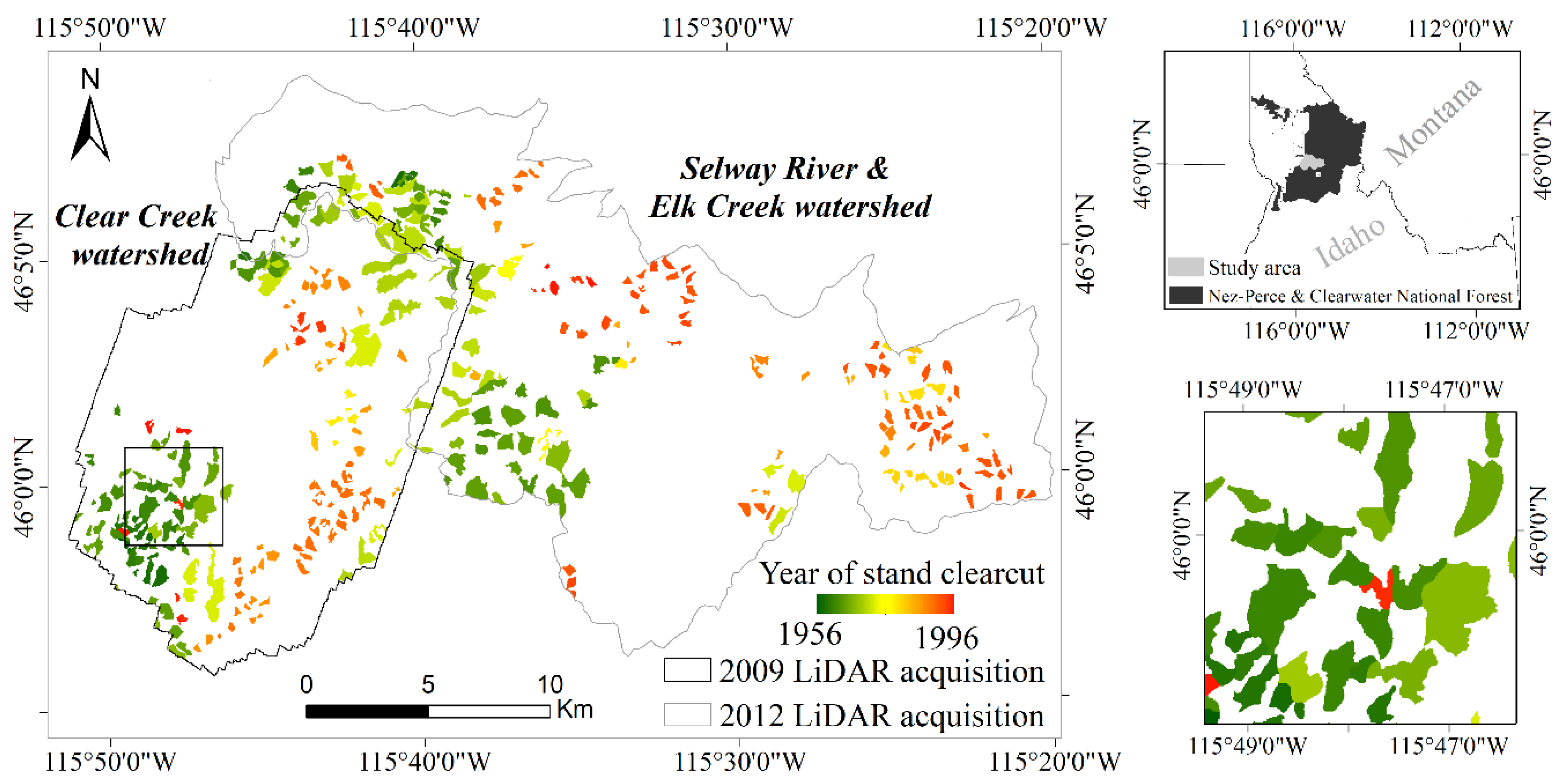
The study area encompasses the Clear Creek, Selway River, and Elk Creek watersheds (~54,000 ha; Figure 1), located within the Nez Perce-Clearwater National Forest (46°48′N, 115°41′W) in north-central Idaho, USA. The study area covers mostly mountainous terrain, with slopes commonly higher than 50%; elevation is highly variable ranging from 415 to 2077 m. Average annual precipitation is around 740 mm; monthly mean temperature is −3.6 °C in winter and 14.2 °C in summer [36]. The area is covered by a temperate mixed-conifer forest. Dominant tree species are Douglas-fir (Pseudotsuga menziesii (Mirb.) Franco.) and grand fir (Abies grandis (Douglas ex D. Don) Lindl.), commonly accompanied by western redcedar (Thuja plicata Donn ex D. Don) and ponderosa pine (Pinus ponderosa C. Lawson). Other species are only sporadically present.
Timber management in the study area initiated early in the twentieth century, but the total amount of timber harvested was relatively small until the 1940s [37]; the area subsequently was intensively logged during the 1960s and 1970s, followed by a phased reduction in logging activity until present. Clearcuts and shelterwoods were the preferred management actions, resulting in a patchy landscape of even-aged forest stands [38,39].
2.2. Ancillary Reference Data and Pre-Processing
The Forest Service ACtivity Tracking System (FACTs) harvest dataset was used as an independent source of information for the location and extent of timber harvest areas [39]. The dataset is maintained by the U.S. Forest Service and consists of vector data (polygons) of the area treated as a part of the timber harvest program work, with an indication of the year in which the harvest was performed. The activities are self-reported by the Forest Service Units and consequently, reporting varies by National Forest administrative districts, and different information on planned management activities, historical records and other available data sources such as available cartography, aerial orthophotos, or remotely sensed data are used for its compilation. We selected clearcut harvest units larger than 2 ha present within the boundaries of our study area, resulting in a total of 360 polygons with 17.75 ha average size, logged between 1956 and 1996 (Figure 1).
Figure 1 shows that in many cases adjacent polygons were harvested in consecutive years. Because of the relatively low growth rate of the vegetation in the study area, these stands would have a substantially similar structure. Consequently, adjacent polygons harvested within a short time interval (≤5 years) were merged as exemplified in Figure 2.
2.3. LiDAR Datasets and Data Pre-Processing
Airborne LiDAR data were acquired in 2009 on the Clear Creek watershed (henceforth referred as the Clear Creek area) and in 2012 on the Selway River and Elk Creek watersheds (henceforth referred as the Selway area) (Figure 1). Both datasets were acquired using a Leica ALS60 sensor in multi-pulse mode up to 4 returns per pulse, with a 69,400 Hz pulse rate in the Clear Creek area and at 88,000 Hz in the Selway area. In both cases, the average point density was at least 4 points/m2. The LiDAR data were delivered by the provider in a standard binary format (.las) with points labeled as ground or non-ground returns.
Because of the 3-year time difference between the two LiDAR collections, the two datasets were processed separately. The point cloud was normalized to obtain the height above ground of each LiDAR return using a digital terrain model (DTM) interpolated from the ground returns at 1-m spatial resolution. The FUSION toolkit [40] was used to compute gridded, summary LiDAR metrics at 30 m spatial resolution. The pixel size was selected at 30 m considering the extent of the study area and the average size of the reference forest stands. A total of 36 metrics was computed: 25 measures of vegetation canopy height and 11 measures of canopy density (Table 1). Density strata metrics were computed based on all returns so as not to discard useful information related to canopy complexity contained in the higher order returns (non-first returns). Cover metrics generated from both first returns and all returns were tested, because of some evidence that the former can produce more stable height metrics [41,42], which may be more appropriate when combining datasets.
The number of metrics considered for further analysis was reduced based on their field significance and a user defined correlation threshold as many of them were spatially correlated. The 95th percentile of height (thereafter ‘H95′) was selected as it is highly correlated to stand height and biomass [43,44,45,46], and it is less sensitive to outliers compared to other distributional metrics as the maximum height (MaxH) [47]. On the other hand, the dominant cohort of trees to regenerate after a stand-replacing disturbance will grow tall only after a few decades [48]. A canopy density metric above a relatively high height would be sensitive to both younger stand regeneration patterns (showing clusters of low density of points) and older stands (showing clusters of high density of points). Accordingly, the percentage of points above 30 m (thereafter ‘Stratum above 30 m’) was also selected for analysis. Pairwise Pearson correlation coefficients (R) between these two metrics and all other 34 metrics were computed; and only the metrics with average absolute value of R lower than 0.5 (i.e., |R| < 0.5) both with ‘H95′ and ‘Stratum above 30 m’ were retained for the following steps of the analysis. All selected metrics were normalized between 0 and 100.
3. Methods
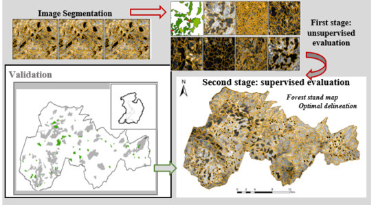
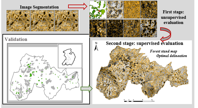
The overall workflow of the proposed methodology is presented in Figure 4. The methodology involves: (1) The single-layer segmentation of several LiDAR metrics (Section 3.1); (2) an object-based unsupervised evaluation to calibrate the segmentation algorithm parameters of each LiDAR metric (Section 3.2); and (3) a supervised evaluation to select the optimal input LiDAR metric for the delineation of forest stands (Section 3.3). An independent validation (Section 3.4) is performed to assess the accuracy of the optimal forest stand delineation.
3.1. Segmentation
Image segmentation of the seven LiDAR metrics was carried out using the multiresolution segmentation (MRS) algorithm [49] implemented in eCognition 9.1 software.
The MRS is a bottom-up segmentation algorithm which starts with a single selected pixel, and merges neighboring pixels into bigger objects in a step-wise iterative process. A detailed description of the algorithm, which is one of the most commonly used algorithms in image segmentation of remotely sensed data within the GEOBIA domain, is provided by Baatz and Schape [49]; the eCognition implementation requires three user-defined parameters: Scale, shape, and compactness. The scale parameter (unitless, unbounded, and defined positive) controls the maximum heterogeneity within the objects; higher scale parameter values hence result in bigger objects. The shape and compactness parameters (unitless, with values defined between 0 and 1) control the border smoothness and compactness of the objects. For each selected LiDAR metric, we generated a set of segmentations by systematically varying the values of the three parameters. The range of variation of the three parameters established to ensure a full range of outputs ranging from undersegmentation to oversegmentation: 91 values of the scale parameter were used, ranging from 5 to 275 in increments of 3 units; three values (0.1, 0.5, and 0.9) were used for shape and compactness.
All the possible combinations of the three sets of values were tested, thus for each LiDAR metric and LiDAR dataset, a total of 819 segmentations was obtained.
3.2. Selection of the Optimal Segmentation of each LiDAR Metric
An unsupervised evaluation method based on spatial autocorrelation statistics was used for selecting the optimal segmentation for each LiDAR metric, out of the 819 generated with the sets of parameters defined above. The method is an adaptation of the one introduced by Espindola et al. [25] and subsequently used for object-based image segmentation evaluation of land cover and stand mapping [26,31,50].
Given a set of segmentations of the same image, the optimal segmentation is defined as the one that maximizes intra-segment homogeneity (i.e., the pixels belonging to the same segment are similar to each other) and inter-segment heterogeneity (i.e., neighboring segments are different from each other).
The intra-segment homogeneity is measured by the weighted variance ():
where and are respectively the variance and the area of segment i, and n is the total number of segments. The upper bound of is equal to the variance of the image when only one image object is part of the segmentation; conversely, the lower bound of is be equal to 0 when each pixel in the image constitutes one image object.
The inter-segment heterogeneity is measured by Moran’s I (MI) index:
where is the mean value of segment i, is the mean value of segment j, is the mean of the pixel values of the entire image, and is a neighbor-based matrix assuming value if objects i and j are adjacent otherwise . can assume values between −1 and 1: Values close to 1 represent clumped patterns with high spatial autocorrelation; values close to 0 represent random patterns; and values close to −1 represent dispersed patterns lacking spatial autocorrelation. was retrieved using the moran function on the R spdep package [51].
Once and are calculated for all the segmentations of the same LiDAR metric, the scores are normalized as proposed by Böck et al. [52]. The weighted variance was normalized respective to the variance of the entire LiDAR metric image used as segmentation input:
where is the weighted variance for the segmentation, and is the variance of the entire image used as segmentation input. Because may vary between 0 and , assumes values between 0 and 1.
was rescaled to the same 0–1 interval as follows:
The two normalized measures are then combined in a single measure, termed Global Score (GS) by Johnson and Xie [26], and proposed as an objective function to rank the set of segmentation outputs and select the one resulting in the lowest GS. The original formulation of GS is a simple linear combination of and ; in order to avoid cases where the lowest GS is attained by a segmentation that is clearly undersegmenting (high but very low ) or oversegmenting (high but very low ), we propose the use of a quadratic cost function, that privileges segmentations with balanced intra-segment homogeneity and inter-segment heterogeneity:
assumes values in the 0 to 1 range: values close to 0 being indicative of high intra-segment homogeneity and inter-segment heterogeneity; and values close to 1 being indicative of low intra-segment homogeneity and inter-segment heterogeneity.
For each of the seven LiDAR metrics considered, the segmentation with the lowest was selected as optimal.
3.3. Selection of the Optimal LiDAR Metric
The second stage of the proposed methodology is to identify, among the set of seven optimal segmentations, the one that most closely matches even-aged stands as they are in reality, i.e., selecting which LiDAR metric is mostly suitable for forest stand delineation. A supervised evaluation method was used, based on measures of area dissimilarity between the segments (henceforth, image objects) and the FACTs harvest dataset, used as a reference map of even-aged forest stands (henceforth, reference objects).
Several metrics have been proposed in the literature as measures of area correspondence between image objects and reference objects [16,21,53,54,55,56,57,58,59]; these methods generally quantify oversegmentation and undersegmentation of the image objects. Oversegmentation happens when an identified reference object results in too many smaller image objects after the segmentation process. Conversely, undersegmentation occurs when the image object spatially matches with more than one of the reference objects, the image object being larger in size compared to the target feature of interest. An ideal, error-free segmentation would have no oversegmentation and no undersegmentation. In reality, each classification have some oversegmentation and some undersegmentation: The selection of the optimal segmentation is therefore based on a ranking strategy that balances the two types of error [21].
The adopted supervised evaluation method is based on measures of area dissimilarity proposed by Clinton et al. [21]. We define as the set of all the image objects, and as the set of all the reference objects. For each reference object , is the set of corresponding image objects, defined as all image objects of whose area overlaps by more than 50% with the reference object (i.e., ); or conversely if the reference object overlaps more than half of the segmented object (i.e., ) [58]. This 50% overlapping area criterion has been consistently used as an appropriate threshold for object-based quality assessment [21,27,54].
The measures of oversegmentation (OS) and undersegmentation (US) [21] are calculated by starting with pair-wise comparisons between image objects and corresponding reference objects, which are then summarized for the entire image.
For each image object , and corresponding reference object the oversegmentation ( is calculated as the fraction of overlapping area relative to the area of the reference object:
Conversely, undersegmentation is calculated as the fraction of overlapping area, relative to the area of the image object:
is then aggregated into the overall oversegmentation of object :
and is aggregated as the total oversegmentation of the n reference objects:
Likewise, is aggregated into the overall undersegmentation of object :
and is aggregated as the total undersegmentation of the n reference objects:
To select the optimal metrics, OS and US were combined into a summary score (D):
In the cases where no corresponding objects for a specific reference object were found according to the defined 50% overlapping area criterion (i.e., , and were given a value of 1.
Once the optimal segmentations of each LiDAR metric were evaluated, the LiDAR metric whose segmentation results in the lowest D score was selected as optimal.
In order to investigate whether the same metric results in the optimal segmentation regardless of time since disturbance, the metrics of area agreement were computed using as reference objects different subsets of the FACTS harvest polygons, resulting in four scenarios:
- All clearcuts (years from 1956 to 1996);
- clearcuts performed before the start of the Landsat MSS record (years from 1956 to 1972);
- clearcuts performed before the start of the Landsat TM record (years from 1956 to 1984);
- clearcuts performed after the start of the Landsat TM record (years from 1984 to 1996).
The four scenarios are driven by the Landsat data archive since it is the longest available Earth Observation record, starting with the launch of Landsat-1 in 1972.
3.4. Validation
The segmentation selected through the two-stage semi-automatic procedure was validated by comparing it to a randomly selected set of reference objects, derived from visual interpretation. The accuracy of the segmentation was assessed using area-based dissimilarity measures.
3.4.1. Reference Dataset
The FACTS dataset is a valuable record of historical disturbances, but it is not intended to be a wall-to-wall map of stand boundaries. While the presence of a polygon indicates a documented, historical clearcut, the absence of a polygon might indicate the absence of historical data, rather than an undisturbed stand. For this reason, an independent reference dataset encompassing both even-aged (EAF) and undisturbed uneven-aged (UAF) forest stands was developed. Reference objects were delineated through visual interpretation of the 1-m spatial resolution digital orthophotos acquired from the National Agricultural Imagery Program (NAIP). Tri-dimensional renderings of the normalized LiDAR point clouds, as well as the raster LiDAR metrics, were used as additional data sources in the interpretation. NAIP imagery acquired in 2009 was used for the Clear Creek dataset, and 2011 imagery (closer in time to the LiDAR flight) was used for the Selway dataset.
The reference objects were generated as follows:
- Random selection of an image object of the optimal segmentation, to account for the large disparity in stand area, followed by random selection of a point within the object [60];
- visual interpretation of the NAIP imagery to trace the forest stand that includes the point. Any physical barriers such as roads or watersheds were used to delineate the border of the stands when no other natural discontinuity related to vegetation type or structure was found;
- classification of the reference object as EAF or uneven-aged forest by the photo-interpreter.
A total of 100 reference objects were generated: 25 EAF and 25 UAF objects for each of the two study areas.
3.4.2. Validation Metrics
The validation metrics used to characterize the agreement and disagreement between image objects and reference objects are:
- Oversegmentation (OS), undersegmentation (US) and summary score (D), obtained with the procedure described in Section 4.3;
- modified oversegmentation (), undersegmentation (), and summary score (), defined as follows.
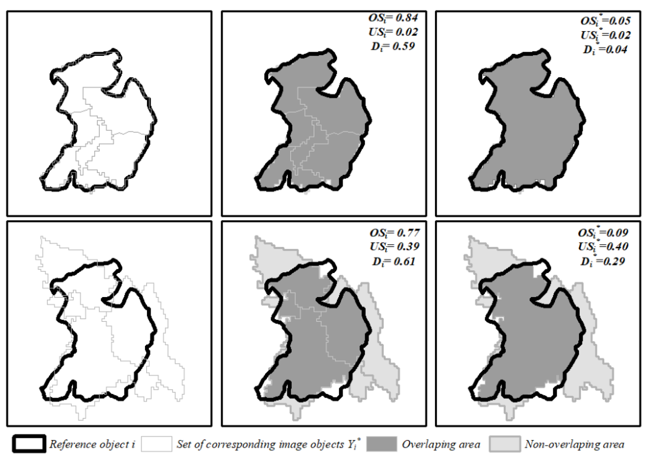
The modified area-based dissimilarity metrics ( are defined as the benchmark value of (OS, US, D), that could be achieved in the best case scenario when the image objects identified by the segmentation are post-processed and merged through object-based classification. The issue is illustrated in Figure 5, where two significantly different segmentations are compared to the same reference object. The top row shows a case of oversegmentation, where an almost perfect match could be achieved through classification, if all the corresponding image objects are merged. Conversely, the bottom row shows a case of where significant discrepancies could not be resolved through classification of the image objects. This is reflected by the modified metrics (Figure 5, right column) where ( represent the areal disagreement between the reference object and the best possible aggregation of the image objects. The modified metrics are significant for the specific application of forest stand mapping, where the segmentation should not be seen as an end-product per se, but as an input dataset for further classification of forest characteristics. We expect the difference between (OS, US, D) and (OS*, US*, D*) to be particularly significant on UAF stands, that due to their larger size and heterogeneity compared to EAF are expected to show a high degree of oversegmentation, that might be however resolved through post-processing.
The modified metrics are computed by considering, instead of the single image objects corresponding to a reference object , their union defined as:
being the subset set of corresponding image objects defined considering the 50% overlapping area criterion described in Section 4.3; by definition is the best possible result of a post-processing of the segmentation.
For each reference object the modified oversegmentation is calculated as the fraction of overlapping area with relative to the area of the reference object:
(14) is then aggregated into an overall oversegmentation metric for the entire set of n reference objects:
Similarly, the modified undersegmentation is calculated for each reference object as:
and (16) is aggregated into an overall undsersegmentation metric:
Finally, the modified summary score is calculated as the quadratic cost function of and :
4. Results
4.1. Selection of the Optimal Segmentation of each LiDAR Metric
The procedure described in Section 4.2 was used for the evaluation of the 819 segmentations obtained for each LiDAR metric using different sets of MRS algorithm parameters (scale, shape, and compactness). Figure 6 illustrates, using the ‘H95′ metric as an example, that different scale and shape parameters influence the number, shape, and size of the segments, as discussed in [49].
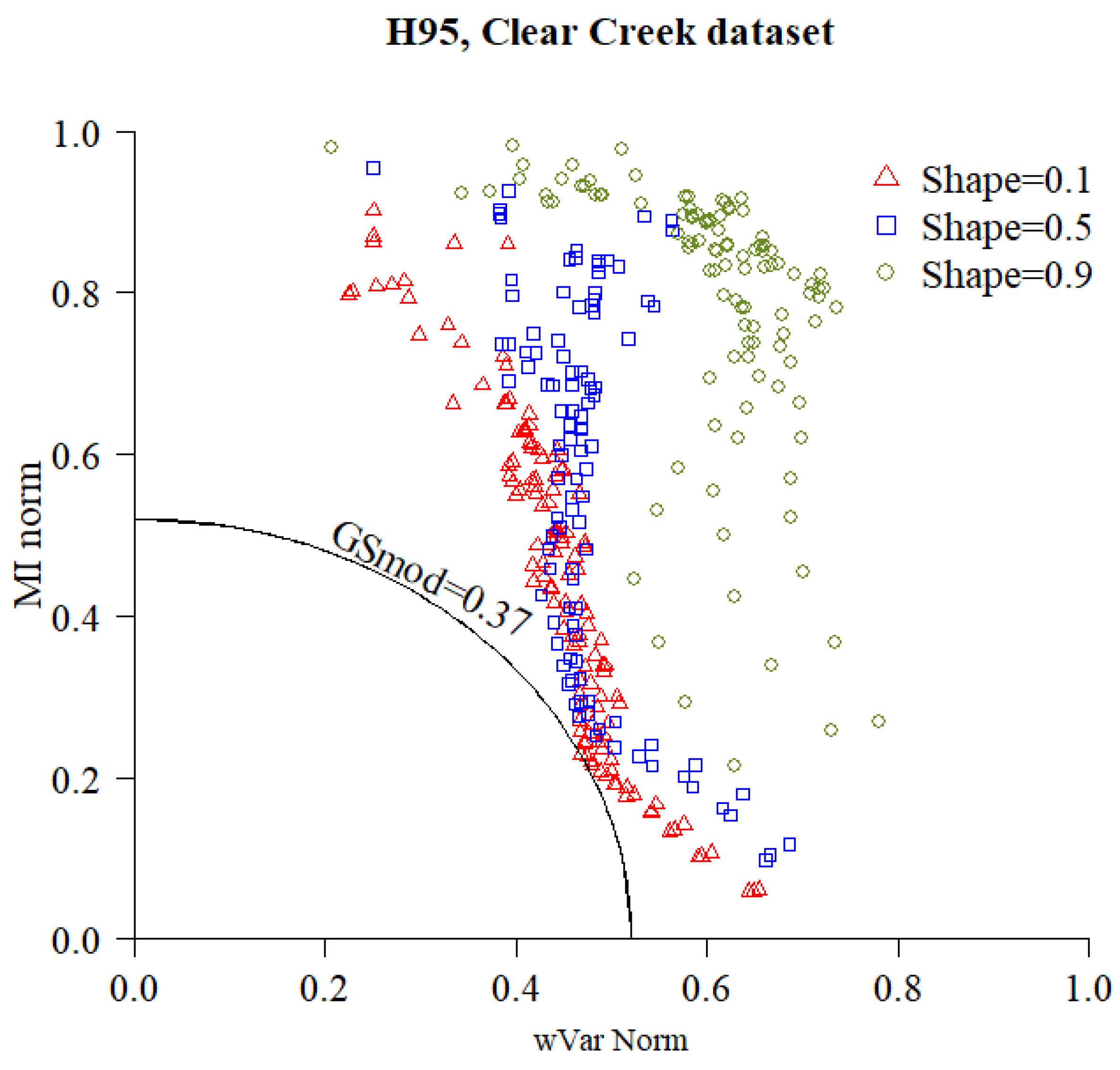
The measures of spatial autocorrelation (, ) were computed for each segmentation, and the summary score () was used for ranking them. Figure 7 exemplifies the procedure for the selection of the optimal segmentation, showing the scatter-plot of the and value of each segmentation of the ‘H95′ LiDAR metric of the Clear Creek dataset, as well as the isoline corresponding to the optimal segmentation.
In general, for each LiDAR metric, the parameters that generate the optimal segmentation on both datasets are very similar (Table 3). For instance, the shape is always 0.1, and the scale parameter between both datasets never differ more than a scale increment of 3 units. A notable exception is the ‘Stratum above 30 m’ metric, where the optimal scale parameter is 59 on the Clear Creek dataset and 23 on the Selway dataset. This difference can be explained considering the low sensitivity of this metric to vegetation recovery: the percentage of returns above 30 m will remain negligible until the top of the trees is higher than 30 m, which might take several decades after a stand-replacing disturbance. In the Clear Creek area many clearcuts are adjacent or spatially close to each other (Figure 1); because of the low sensitivity of the metric, there is no clear distinction in the “Stratum above 30 m” metric between neighboring disturbed stands, and the optimal segmentation is the one identifying these very large image objects. Figure 1 shows that the clearcuts of the Selway area are instead surrounded by undisturbed stands, generating a more heterogenous patchy landscape that create recognizable stand boundaries despite the low sensitivity of the ‘Stratum above 30 m’ metric.
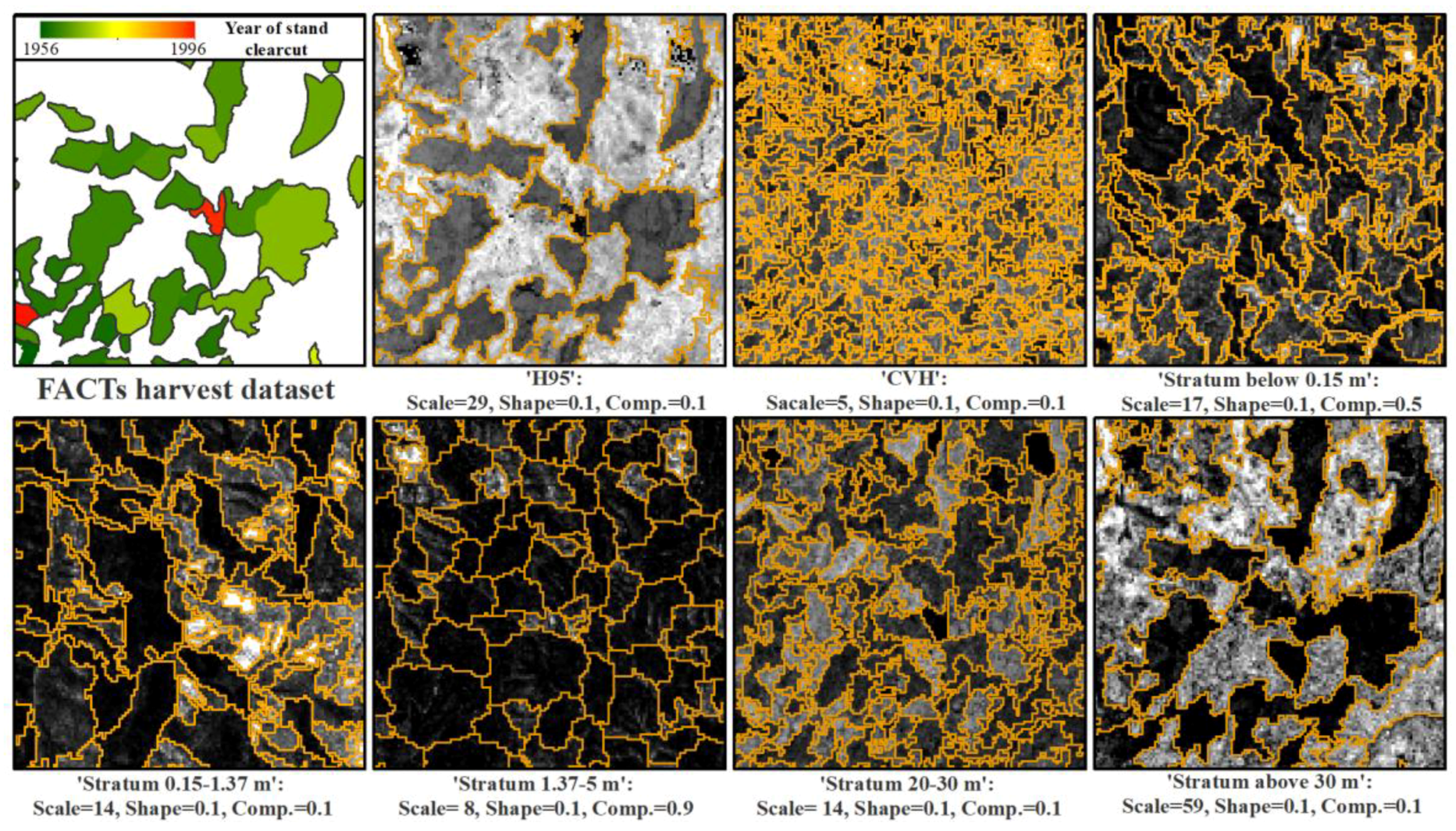
Figure 8 illustrates that the optimal segmentation of different LiDAR metrics might show very different vegetation-related structural objects. While in general the image objects that can visually recognized in each of the LiDAR metrics are delineated by the optimal segmentation, not all metrics return image objects that match the historic disturbances reported by the FACTS dataset. Figure 8 shows that the ‘H95′ and ‘Stratum above 30 m’ visually match closely the FACT dataset, whereas the other metrics define image objects that do not immediately relate to the record of past clearcuts.
4.2. Selection of the Optimal LiDAR Metric
The optimal segmentation of each LiDAR metric was compared against the reference objects from the FACTs harvest dataset following the procedure described in Section 3.3; the results of the analysis, for the two study areas and for the four scenarios of time since disturbances, are summarized in Table 4. The ‘H95′ metric results in the lowest D value for both datasets in all but one case (Table 4), namely when considering only the most recent disturbances (1984–1996) on the Clear Creek dataset. In this case, the ‘Stratum 20–30 m’ metric results in the lowest score (D = 22), with the ‘H95′ metric having the second lowest score (D = 0.25). Conversely, the ‘Stratum 20–30 m’ metric is the second-best metric of the remaining three scenarios in the Clear Creek area, and the ‘Stratum above 30 m’ is always the second-best metric in the Selway area. Additionally, the optimal segmentation of the ‘H95′ metric is the only one where all the reference objects have a non-null set of matching image objects (i.e., ) (Table 4).
The ‘H95′ LiDAR metric was therefore selected as the optimal metric. Figure 9 shows the segmentation of the ‘H95′ LiDAR metric as the optimal delineation for even-aged forest stand mapping in the study area.
4.3. Validation
One hundred reference objects were manually delineated (Figure 10 and Figure 11) to validate the optimal segmentation results, as described in Section 3.4. This sample size corresponds to 8% of the total number of image objects identified by the optimal segmentation (1182 objects in total, as reported in Table 3), and the resulting reference dataset covers 16% of the surface of the study area. The reference sample size is comparable with previous GEOBIA-based studies [27,54,61].
The independent validation performed with the visually interpreted polygons representing both EAF and UAF stands confirmed the good match between image objects and forest stands. On EAF stands, in particular, in most cases there was a 1-to-1 correspondence between the EAF reference objects and the set of corresponding image objects; whereas UAF reference objects were generally undersegmented, and corresponded to several image objects (Figure 10). The validation also showed that, in a few isolated cases, the ‘H95′ metric has an abnormal behavior on very recent clearcuts, as in the example of Figure 11, third row, where a recently harvested stand is not visible in the LiDAR raster. This is due to the specific definition of the ‘H95′ metric (Table 1): In the absence of vegetation regrowth the majority of returns are classified as ‘ground’, and the 95th percentile of the non-ground returns corresponds to the height of isolated trees left standing for seedling after the clearcut.
The area based dissimilarity metrics, reported in Table 5, indicate that the overall performance (summarized by the D score) is very similar across the two datasets (= 0.26 and when considering all objects), with consistently higher accuracy on EAF stands ( = 0.15 and = 0.16) than on UAF stands ( and ). This difference is largely due to the high rates of oversegmentation on UAF stands in both datasets ( vs. ; and vs. ).
As discussed in Section 3.4.2, the modified metrics (, , ) represent the benchmark level of error that could be achieve through the best possible post-processing of the segmentation. The modified metrics indicate that post-processing has the potential to significantly reduce the areal disagreements due to oversegmentation, especially over UAF stands ( vs. vs. ).
5. Discussion
In the present paper we propose the integration in the same workflow of an object-based unsupervised evaluation (which allows for the selection of the optimal parameters to automatically segment an image) and an object-based supervised evaluation (which allows for the selection of the best match between a segmentation and independently derived reference objects) to identify objectively an optimal delineation output. Unsupervised methods favor automatic ranking of multiple segmentations obtained by changing the parameters of an algorithm on the same input data, without requiring any contribution from the operator, or any external datasets. They do not, however, allow for ranking segmentations obtained on the same area from different input data, as in the case of the LiDAR raster metrics examined in this paper, which reflect different structural characteristics of the vegetation, as evident in Figure 3. Supervised evaluation methods instead allow for ranking any segmentation—whether it is generated from the same image or not—but rely entirely on reference data, whose generation is generally an expensive and time-consuming task [62]. As a consequence, supervised evaluation methods are generally employed only on relatively small datasets [26]. The combination of these two standard object-based evaluation strategies, as proposed in this paper, reduces considerably the amount of required reference data and increases the scope of a reliable semi-automatic delineation to larger areas.
The application of the proposed methodology to LiDAR data demonstrates that a single LiDAR raster metric, the ‘H95′ metric, can be used to delineate even-aged forest stands in a semi-automatic way. In particular, the results show that forest stands harvested in the 1950s and 1960s can still be accurately delineated (Table 4). This result is particularly significant, because it implies that LiDAR data can be potentially used to reconstruct the disturbance history of a forest extending beyond the optical satellite data record.
The optimal segmentation was validated against a randomly selected reference dataset. The reference objects were manually delineated by a skilled photo-interpreter, based on imagery of higher resolution (1 m NAIP data) and richer thematic content (3D LiDAR point clouds) than the 30 m LiDAR raster. While there is a degree of subjectivity, visually interpreted reference data are commonly used for the validation of land cover and land cover disturbance satellite products (e.g., [63,64]), and for the validation of GEOBIA outputs (e.g., [26,27,31,34,54,61]).
The independent validation confirmed the good overall match between image objects and visually interpreted polygons, albeit with higher accuracy on EAF than on UAF forest stands. At least in part, the low accuracy on UAF stands might be attributed to the lack of objective UAF stand definition, and to the difficulty for the interpreter to consistently identify natural breaks between contiguous, mature, uneven-aged forest stands. The validation also highlighted some limitations of the ‘H95′ metric. The optimal segmentation showed undersegmentation errors (e.g., Figure 11, third row) on small stands recently (<10 year) harvested, where mature trees are left standing at regular intervals to spread seeds (e.g., shelterwood cutting). At time of the LiDAR acquisition the majority of the young regenerating seedlings have a height below 1.37 m (the cutoff used for the raster height metrics), and the ‘H95′ metric therefore reflects the height of the mature trees left standing. We hypothesize that the combined use of multiple LiDAR metrics (such as the ‘Stratum 20–30 m’ which ranked second in the supervised evaluation) might overcome this particular issue.
Previous research to delineate structural or age-related forest stand types using object-based techniques and LiDAR data (e.g., [2,10,11,31,34,35]) did not propose methodologies that could be easily applied outside the original study areas, due to the complexity of the workflow (e.g., [10]), to the exploitation of site-specific forest characteristics and to the small extent of the study areas (e.g., [2,11,34,35]), and to the lack of objective evaluation protocols (e.g., [2,11]). The proposed two-stage evaluation strategy is a general objective workflow, that could be easily replicated and adapted to other study sites, to other data sources, and to delineate different features of the landscape. Overall, we expect that the same ‘H95′ metric could be optimal, at the working resolution, in other areas with similar species composition and with similar disturbance dynamics (such as most of the Pacific Northwest of the United States), and that the optimal set of parameters of the MRS algorithm for each area could be identified through an unsupervised selection procedure, hence without the need for additional independent reference data. Additional validation would be required to verify whether the same LiDAR metric could be also used for delineating forest stands resulting from disturbances and management practices other than clearcuts. Future research will (1) evaluate a different set of single or combined LiDAR metrics for segmentation (e.g., texture metrics, rumple index, local maxima derived from the CHM); and (2) develop a rule-based fusion between segmentations generated from complementary metrics and different harvest treatments, as some limitations in the detection of recent disturbances has been observed after the independent validation was addressed.
6. Conclusions
This paper proposes a two-stage, semi-automatic evaluation strategy for object-based forest stand delineation and implements it on two contiguous LiDAR datasets covering more than 54,000 ha in the Clear Creek and Selway watersheds in Central Idaho. The paper was designed to address two main objectives: (1) To integrate a straightforward and objective workflow for forest stand delineation that can be easily replicated and adapted at regional scales; and (2) to evaluate the performance of commonly used rasterized LiDAR metrics, such as ‘H95′ in this study, to identify in a semi-automatic way the boundaries of relatively old even-aged forest stands.
With regards to the first objective, the proposed strategy allows the user to automatically select the optimal set of MRS algorithm segmentation parameters to delineate image objects for each tested LiDAR metric, and to identify the LiDAR metric that ensures the best match between image objects (i.e., the segmentation) and a set of reference objects (i.e., the forest stands as independently delineated). With regards to the second objective, the application of the methodology to LiDAR data demonstrates that commonly used LiDAR raster metrics, namely distributional metrics of canopy height, can be used to accurately delineate even-aged forest stands (>2 ha) in a semi-automatic way and that forest stands older than 50 years can be identified at working resolution of 30 m. This is a particularly significant result, considering that stand maps conventionally generated from change detection using optical satellite data can only extend, in the best case, to the beginning of the Landsat MSS record in 1972.
GEOBIA strategies to delineate forest stands at regional scales are promising to generate forest stands maps ready to use, but generalized protocols are still required. The most effective way to approach the delineation would depend on the adopted definition of a forest stand (e.g., based on species composition, structure, etc.). In any case, robust evaluation strategies would be required to assure a minimum quality on the final selected output. We proposed here a straightforward and objective two-stage evaluation workflow to delineate forest stands defined in terms of age and structural homogeneity. Our study shows that relatively old stands are accurately discriminated using one single-date LiDAR raster metric, which is promising result not only to produce even-aged forest stand maps but also to eventually characterize forest stands in terms of time since the last disturbance. Additionally, this methodology can be adapted to address future study needs, such as to improve stand delineation methods, or to map other geographic features of the landscape.
Author Contributions
N.S.-L., L.B., and A.T.H. conceived the overall approach of the paper. N.S.-L. refined the methods, process the data and wrote the draft of the paper with assistance from L.B., A.T.H. provided technical assistance, comments and feedback while drafting and finalizing the manuscript.
Funding
The project is supported by NASA award number NHX14AD92G and by USDA NIFA grant number 2011-32100-06016. Publication of this article was funded by the University of Idaho Open Access Publishing Fund.
Conflicts of Interest
The authors declare no conflict of interest.
References
- Leckie, D.G.; Gougeon, F.A.; Walsworth, N.; Paradine, D. Stand delineation and composition estimation using semi-automated individual tree crown analysis. Remote Sens. Environ. 2003, 85, 355–369. [Google Scholar] [CrossRef]
- Sullivan, A.A.; McGaughey, R.J.; Andersen, H.-E.; Schiess, P. Object-oriented classification of forest structure from light detection and ranging data for stand mapping. West. J. Appl. For. 2009, 24, 198–204. [Google Scholar]
- Helms, J. The Dictionary of Forestry; Western Heritage Co.: Loveland, CO, USA, 1998. [Google Scholar]
- Masek, J.G.; Goward, S.N.; Kennedy, R.E.; Cohen, W.B.; Moisen, G.G.; Schleeweis, K.; Huang, C. United States Forest Disturbance Trends Observed Using Landsat Time Series. Ecosystems 2013, 16, 1087–1104. [Google Scholar] [CrossRef] [Green Version]
- White, J.C.; Wulder, M.A.; Hermosilla, T.; Coops, N.C.; Hobart, G.W. A nationwide annual characterization of 25 years of forest disturbance and recovery for Canada using Landsat time series. Remote Sens. Environ. 2017, 194, 303–321. [Google Scholar] [CrossRef]
- Leckie, D.G.; Gillis, M.D. Forest inventory in Canada with emphasis on map production. For. Chron. 1995, 71, 74–88. [Google Scholar] [CrossRef] [Green Version]
- Fisher, R.A.; Koven, C.D.; Anderegg, W.R.; Christoffersen, B.O.; Dietze, M.C.; Farrior, C.E.; Holm, J.A.; Hurtt, G.C.; Knox, R.G.; Lawrence, P.J. Vegetation demographics in Earth System Models: A review of progress and priorities. Glob. Chang. Biol. 2018, 24, 35–54. [Google Scholar] [CrossRef] [PubMed]
- Burnett, C.; Blaschke, T. A multi-scale segmentation/object relationship modelling methodology for landscape analysis. Ecol. Model. 2003, 168, 233–249. [Google Scholar] [CrossRef]
- Dechesne, C.; Mallet, C.; Le Bris, A.; Gouet-Brunet, V. Semantic segmentation of forest stands of pure species combining airborne lidar data and very high resolution multispectral imagery. ISPRS J. Photogramm. Remote Sens. 2017, 126, 129–145. [Google Scholar] [CrossRef]
- Koch, B.; Straub, C.; Dees, M.; Wang, Y.; Weinacker, H. Airborne laser data for stand delineation and information extraction. Int. J. Remote Sens. 2009, 30, 935–963. [Google Scholar] [CrossRef]
- Pascual, C.; García-Abril, A.; García-Montero, L.G.; Martín-Fernández, S.; Cohen, W.B. Object-based semi-automatic approach for forest structure characterization using lidar data in heterogeneous Pinus sylvestris stands. For. Ecol. Manag. 2008, 255, 3677–3685. [Google Scholar] [CrossRef]
- Tiede, D.; Blaschke, T.; Heurich, M. Object-based semi automatic mapping of forest stands with Laser scanner and Multi-spectral data. Int. Arch. Photogramm. Remote Sens. Spat. Inf. Sci. 2004, 36, 328–333. [Google Scholar]
- Wulder, M.A.; White, J.C.; Hay, G.J.; Castilla, G. Towards automated segmentation of forest inventory polygons on high spatial resolution satellite imagery. For. Chron. 2008, 84, 221–230. [Google Scholar] [CrossRef] [Green Version]
- Blaschke, T.; Lang, S.; Hay, G. Object-Based Image Analysis: Spatial Concepts for Knowledge-Driven Remote Sensing Applications; Springer Science & Business Media: Berlin, Germany, 2008; ISBN 978-3-540-77058-9. [Google Scholar]
- Blaschke, T.; Hay, G.J.; Kelly, M.; Lang, S.; Hofmann, P.; Addink, E.; Queiroz Feitosa, R.; van der Meer, F.; van der Werff, H.; van Coillie, F.; et al. Geographic Object-Based Image Analysis—Towards a new paradigm. ISPRS J. Photogramm. Remote Sens. 2014, 87, 180–191. [Google Scholar] [CrossRef] [PubMed]
- Costa, H.; Foody, G.M.; Boyd, D.S. Supervised methods of image segmentation accuracy assessment in land cover mapping. Remote Sens. Environ. 2018, 205, 338–351. [Google Scholar] [CrossRef]
- Liu, D.; Xia, F. Assessing object-based classification: Advantages and limitations. Remote Sens. Lett. 2010, 1, 187–194. [Google Scholar] [CrossRef]
- Walter, V. Object-based classification of remote sensing data for change detection. ISPRS J. Photogramm. Remote Sens. 2004, 58, 225–238. [Google Scholar] [CrossRef]
- Zhang, Y.J. A survey on evaluation methods for image segmentation. Pattern Recognit. 1996, 29, 1335–1346. [Google Scholar] [CrossRef]
- Belgiu, M.; Drǎguţ, L. Comparing supervised and unsupervised multiresolution segmentation approaches for extracting buildings from very high resolution imagery. ISPRS J. Photogramm. Remote Sens. 2014, 96, 67–75. [Google Scholar] [CrossRef] [PubMed]
- Clinton, N.; Holt, A.; Scarborough, J.; Yan, L.I.; Gong, P. Accuracy assessment measures for object-based image segmentation goodness. Photogramm. Eng. Remote Sens. 2010, 76, 289–299. [Google Scholar] [CrossRef]
- Neubert, M.; Herold, H.; Meinel, G. Assessing image segmentation quality—Concepts, methods and application. In Object-Based Image Analysis; Blaschke, T., Lang, S., Hay, G.J., Eds.; Lecture Notes in Geoinformation and Cartography; Springer: Berlin/Heidelberg, Germany, 2008; pp. 769–784. ISBN 978-3-540-77057-2. [Google Scholar]
- Zhang, Y.J. Evaluation and comparison of different segmentation algorithms. Pattern Recognit. Lett. 1997, 18, 963–974. [Google Scholar] [CrossRef]
- Johnson, B.A.; Bragais, M.; Endo, I.; Magcale-Macandog, D.B.; Macandog, P.B.M. Image Segmentation Parameter Optimization Considering Within- and Between-Segment Heterogeneity at Multiple Scale Levels: Test Case for Mapping Residential Areas Using Landsat Imagery. ISPRS Int. J. Geo-Inf. 2015, 4, 2292–2305. [Google Scholar] [CrossRef] [Green Version]
- Espindola, G.M.; Camara, G.; Reis, I.A.; Bins, L.S.; Monteiro, A.M. Parameter selection for region-growing image segmentation algorithms using spatial autocorrelation. Int. J. Remote Sens. 2006, 27, 3035–3040. [Google Scholar] [CrossRef]
- Johnson, B.; Xie, Z. Unsupervised image segmentation evaluation and refinement using a multi-scale approach. ISPRS J. Photogramm. Remote Sens. 2011, 66, 473–483. [Google Scholar] [CrossRef]
- Drăguţ, L.; Csillik, O.; Eisank, C.; Tiede, D. Automated parameterisation for multi-scale image segmentation on multiple layers. ISPRS J. Photogramm. Remote Sens. 2014, 88, 119–127. [Google Scholar] [CrossRef] [PubMed]
- Gao, H.; Tang, Y.; Jing, L.; Li, H.; Ding, H. A Novel Unsupervised Segmentation Quality Evaluation Method for Remote Sensing Images. Sensors 2017, 17, 2427. [Google Scholar] [CrossRef] [PubMed]
- Georganos, S.; Lennert, M.; Grippa, T.; Vanhuysse, S.; Johnson, B.; Wolff, E. Normalization in Unsupervised Segmentation Parameter Optimization: A Solution Based on Local Regression Trend Analysis. Remote Sens. 2018, 10, 222. [Google Scholar] [CrossRef]
- Gonzalez, R.S.; Latifi, H.; Weinacker, H.; Dees, M.; Koch, B.; Heurich, M. Integrating LiDAR and high-resolution imagery for object-based mapping of forest habitats in a heterogeneous temperate forest landscape. Int. J. Remote Sens. 2018, 1–26. [Google Scholar] [CrossRef]
- Varo-Martínez, M.Á.; Navarro-Cerrillo, R.M.; Hernández-Clemente, R.; Duque-Lazo, J. Semi-automated stand delineation in Mediterranean Pinus sylvestris plantations through segmentation of LiDAR data: The influence of pulse density. Int. J. Appl. Earth Obs. Geoinf. 2017, 56, 54–64. [Google Scholar] [CrossRef]
- Dechesne, C.; Mallet, C.; Le Bris, A.; Gouet, V.; Hervieu, A. Forest stand segmentation using airborne lidar data and very high resolution multispectral imagery. ISPRS Arch. Photagramm. Remote Sens. 2016, 41, 207–214. [Google Scholar] [CrossRef]
- Ke, Y.; Quackenbush, L.J.; Im, J. Synergistic use of QuickBird multispectral imagery and LIDAR data for object-based forest species classification. Remote Sens. Environ. 2010, 114, 1141–1154. [Google Scholar] [CrossRef]
- Leppänen, V.J.; Tokola, T.; Maltamo, M.; Mehtätalo, L.; Pusa, T.; Mustonen, J. Automatic delineation of forest stands from LiDAR data. In GEOBIA, 2008—Pixels, Objects, Intelligence: GEOgraphic Object Based Image Analysis for the 21st Century; University of Calgary: Calgary, AB, Canada, 2008; pp. 271–277. [Google Scholar]
- Wu, Z.; Heikkinen, V.; Hauta-Kasari, M.; Parkkinen, J.; Tokola, T. ALS data based forest stand delineation with a coarse-to-fine segmentation approach. In Proceedings of the 2014 7th International Congress on Image and Signal Processing, Dalian, China, 14–16 October 2014; pp. 547–552. [Google Scholar]
- Hijmans, R.J.; Cameron, S.E.; Parra, J.L.; Jones, P.G.; Jarvis, A. Very high resolution interpolated climate surfaces for global land areas. Int. J. Climatol. 2005, 25, 1965–1978. [Google Scholar] [CrossRef] [Green Version]
- Cochrell, A.N. The Nezperce Story: A History of the Nezperce National Forest; USDA Forest Service: Missoula, MT, USA, 1960.
- Space, R.S. Clearwater Story: A History of the Clearwater National Forest; United States Department of Agriculture: Washington, DC, USA, 1964.
- USDA, Forest Service Forest Service Activity Tracking System (FACTs) Harvest Database. Available online: http://data.fs.usda.gov/geodata/edw/datasets.php (accessed on 28 November 2017).
- McGaughey, R.J. FUSION/LDV: Software for LIDAR Data Analysis and Visualization; US Department of Agriculture, Forest Service, Pacific Northwest Research Station: Seattle, WA, USA, 2009.
- Næesset, E. Effects of different sensors, flying altitudes, and pulse repetition frequencies on forest canopy metrics and biophysical stand properties derived from small-footprint airborne laser data. Remote Sens. Environ. 2009, 113, 148–159. [Google Scholar] [CrossRef]
- Bater, C.W.; Wulder, M.A.; Coops, N.C.; Nelson, R.F.; Hilker, T.; Nasset, E. Stability of Sample-Based Scanning-LiDAR-Derived Vegetation Metrics for Forest Monitoring. IEEE Trans. Geosci. Remote Sens. 2011, 49, 2385–2392. [Google Scholar] [CrossRef]
- González-Ferreiro, E.; Diéguez-Aranda, U.; Miranda, D. Estimation of stand variables in Pinus radiata D. Don plantations using different LiDAR pulse densities. Forestry 2012, 85, 281–292. [Google Scholar] [CrossRef] [Green Version]
- Heurich, M.; Thoma, F. Estimation of forestry stand parameters using laser scanning data in temperate, structurally rich natural European beech (Fagus sylvatica) and Norway spruce (Picea abies) forests. Forestry 2008, 81, 645–661. [Google Scholar] [CrossRef]
- Hudak, A.T.; Crookston, N.L.; Evans, J.S.; Hall, D.E.; Falkowski, M.J. Nearest neighbor imputation of species-level, plot-scale forest structure attributes from LiDAR data. Remote Sens. Environ. 2008, 112, 2232–2245. [Google Scholar] [CrossRef]
- Næsset, E. Predicting forest stand characteristics with airborne scanning laser using a practical two-stage procedure and field data. Remote Sens. Environ. 2002, 80, 88–99. [Google Scholar] [CrossRef]
- Kane, V.R.; McGaughey, R.J.; Bakker, J.D.; Gersonde, R.F.; Lutz, J.A.; Franklin, J.F. Comparisons between field- and LiDAR-based measures of stand structural complexity. Can. J. For. Res. 2010, 40, 761–773. [Google Scholar] [CrossRef] [Green Version]
- Bartels, S.F.; Chen, H.Y.H.; Wulder, M.A.; White, J.C. Trends in post-disturbance recovery rates of Canada’s forests following wildfire and harvest. For. Ecol. Manag. 2016, 361, 194–207. [Google Scholar] [CrossRef]
- Baatz, M.; Schape, A. Multiresolution Segmentation—An Optimization Approach for High Quality Multi-Scale Image Segmentation; AGIT-Symposium: Salzburg, Austria, 2000. [Google Scholar]
- Kim, M.; Madden, M.; Warner, T.A. Forest Type Mapping using Object-specific Texture Measures from Multispectral Ikonos Imagery. Photogramm. Eng. Remote Sens. 2009, 75, 819–829. [Google Scholar] [CrossRef]
- Bivand, R.; Anselin, L.; Berke, O.; Bernat, A.; Carvalho, M.; Chun, Y.; Dormann, C.F.; Dray, S.; Halbersma, R.; Lewin-Koh, N.; et al. SPDEP: Spatial Dependence: Weighting Schemes, Statistics and Models. R package version 0.5-31. 2011. Available online: http://CRAN.R-project.org/package=spdep (accessed on 13 July 2017).
- Böck, S.; Immitzer, M.; Atzberger, C. On the Objectivity of the Objective Function—Problems with Unsupervised Segmentation Evaluation Based on Global Score and a Possible Remedy. Remote Sens. 2017, 9, 769. [Google Scholar] [CrossRef]
- Levine, M.D.; Nazif, A.M. Dynamic Measurement of Computer Generated Image Segmentations. IEEE Trans. Pattern Anal. Mach. Intell. 1985, PAMI-7, 155–164. [Google Scholar] [CrossRef]
- Liu, Y.; Bian, L.; Meng, Y.; Wang, H.; Zhang, S.; Yang, Y.; Shao, X.; Wang, B. Discrepancy measures for selecting optimal combination of parameter values in object-based image analysis. ISPRS J. Photogramm. Remote Sens. 2012, 68, 144–156. [Google Scholar] [CrossRef]
- Lucieer, A.; Stein, A. Existential uncertainty of spatial objects segmented from satellite sensor imagery. IEEE Trans. Geosci. Remote Sens. 2002, 40, 2518–2521. [Google Scholar] [CrossRef]
- Möller, M.; Lymburner, L.; Volk, M. The comparison index: A tool for assessing the accuracy of image segmentation. Int. J. Appl. Earth Obs. Geoinf. 2007, 9, 311–321. [Google Scholar] [CrossRef]
- Weidner, U. Contribution to the assessment of segmentation quality for remote sensing applications. Int. Arch. Photogram. Remote Sens. Spat. Inf. Sci. 2008, 37, 479–484. [Google Scholar]
- Zhan, Q.; Molenaar, M.; Tempfli, K.; Shi, W. Quality assessment for geo-spatial objects derived from remotely sensed data. Int. J. Remote Sens. 2005, 26, 2953–2974. [Google Scholar] [CrossRef]
- Monteiro, F.C.; Campilho, A.C. Performance Evaluation of Image Segmentation. In Image Analysis and Recognition; Campilho, A., Kamel, M.S., Eds.; Springer: Berlin/Heidelberg, Germany, 2006; Volume 4141, pp. 248–259. ISBN 978-3-540-44891-4. [Google Scholar]
- Radoux, J.; Bogaert, P. Good Practices for Object-Based Accuracy Assessment. Remote Sens. 2017, 9, 646. [Google Scholar] [CrossRef]
- Heenkenda, M.K.; Joyce, K.E.; Maier, S.W. Mangrove tree crown delineation from high-resolution imagery. Photogramm. Eng. Remote Sens. 2015, 81, 471–479. [Google Scholar] [CrossRef]
- Zhang, H.; Fritts, J.E.; Goldman, S.A. Image segmentation evaluation: A survey of unsupervised methods. Comput. Vis. Image Underst. 2008, 110, 260–280. [Google Scholar] [CrossRef] [Green Version]
- Boschetti, L.; Stehman, S.V.; Roy, D.P. A stratified random sampling design in space and time for regional to global scale burned area product validation. Remote Sens. Environ. 2016, 186, 465–478. [Google Scholar] [CrossRef]
- Strahler, A.H.; Boschetti, L.; Foody, G.M.; Friedl, M.A.; Hansen, M.C.; Herold, M.; Mayaux, P.; Morisette, J.T.; Stehman, S.V.; Woodcock, C.E. Global Land Cover Validation: Recommendations for Evaluation and Accuracy Assessment of Global Land Cover Maps; European Communities: Luxembourg, 2006. [Google Scholar]
Figure 1.
Location of the study area in the Nez-Perce & Clearwater National Forest (Idaho-USA); boundaries of the 2009 and 2012 Light Detection and Ranging (LiDAR) acquisitions; and reference polygons of historical stand clearcuts (>2 ha) from the Forest Service Activity Track System (FACTs) harvest dataset. The FACTs polygons are displayed with a rainbow color scale indicating the year of harvest, from 1956 to 1996. No data are available for clearcuts performed before 1956; no clearcuts (>2 ha) were reported from 1996 to the LiDAR acquisition dates. On the bottom right, a 4 × 4 km subset of the Clear Creek watershed.

Figure 2.
Example of pre-processing of the FACTs harvest polygons. Adjacent polygons harvested within a time interval ≤5 years (left) are merged into aggregated polygons (right) that are used as reference objects in all the subsequent steps of the analysis.
Figure 2.
Example of pre-processing of the FACTs harvest polygons. Adjacent polygons harvested within a time interval ≤5 years (left) are merged into aggregated polygons (right) that are used as reference objects in all the subsequent steps of the analysis.
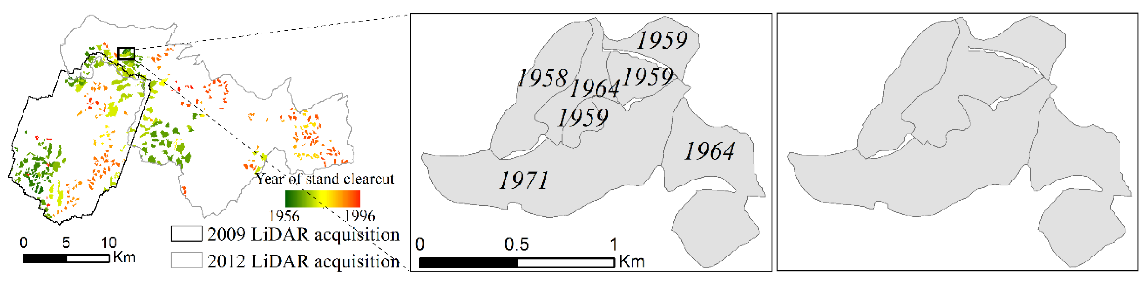
Figure 3.
The seven LiDAR metrics considered in the analysis (Table 2), displayed with a linear black to white grayscale color table (1% linear stretch), on a 4 × 4 km subset of the Clear Creek watershed (location on Figure 1). The FACTs harvest reference dataset is presented for comparison in the upper left, to highlight the different response of each metric to even-aged forest stands.
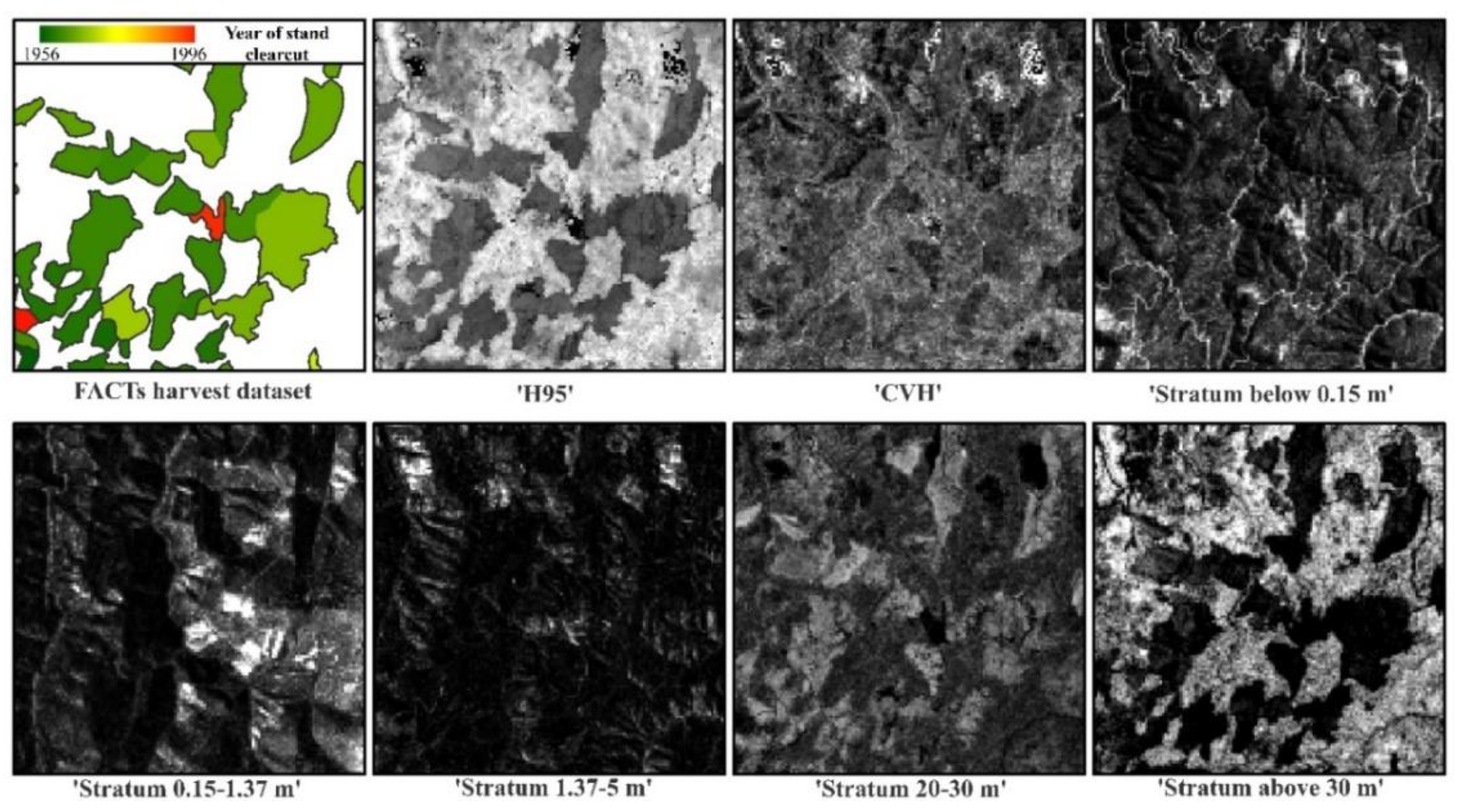
Figure 4.
Flowchart of the proposed methodology for forest stand delineation based on a two-stage evaluation strategy.
Figure 4.
Flowchart of the proposed methodology for forest stand delineation based on a two-stage evaluation strategy.
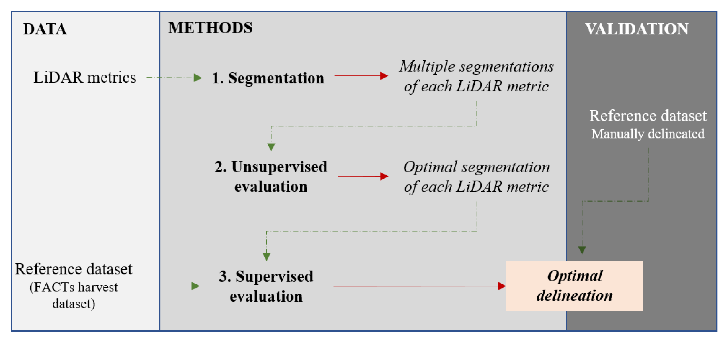
Figure 5.
Illustration of the area-based dissimilarity metrics (, , ), and of the modified metrics (, , ). A reference object (black vectors) is displayed together with its corresponding set of image objects (gray vectors): The top row shows an example where the reference object is oversegmented, but not undersegmented (i.e., it is closely matched by the union area ); the bottom row shows an example where the reference object is both oversegmented, and undersegmented. The center column illustrates the traditional oversegmentation (), undersegmentation () and summary score for that single reference object, metrics that consider each individual corresponding image object. The right column illustrates the modified , , and metrics, that consider instead the union area of all corresponding image objects. The summary score D does not report a significant difference between the two classifications (top: = 0.59, bottom: = 0.61), whereas the modified summary score D* indicates that through post-processing the top row segmentation could result in a near-perfect match with the reference object ( = 0.04) but significant errors will remain in the bottom row segmentation ( = 0.29).

Figure 6.
Segmentations of the ‘H95′ LiDAR metric generated by the multiresolution segmentation (MRS) algorithm with different combinations of the scale and shape parameters, and the same compactness parameter (Comp. = 0.1). In all cases, the segmentation is displayed as orange vectors overlaid on the ‘H95′ metric raster, shown in grayscale. The same 4 × 4 km area of Figure 1 is presented.
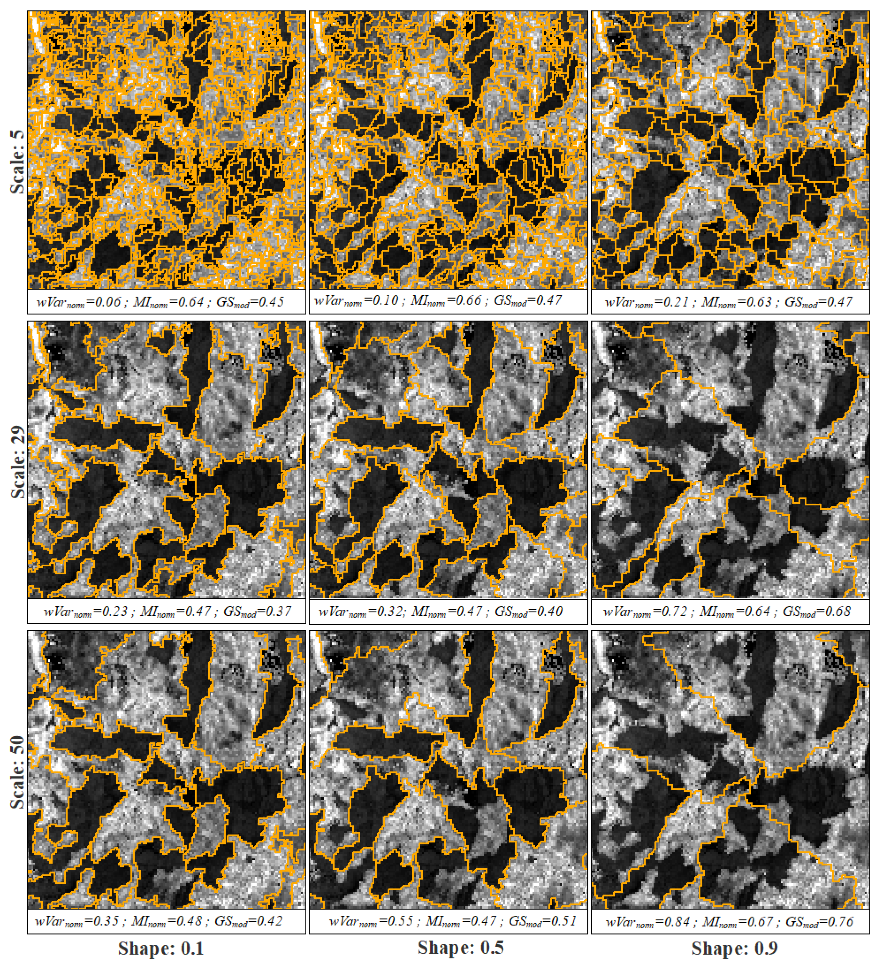
Figure 7.
Scatter-plot of the normalized weighted variance () and normalized Moran’s Index () of the segmentations of the ‘H95′ metric for the Clear Creek dataset, generated by different sets of the MRS algorithm parameters. The two metrics are combined in a quadratic Global Score () and the segmentation with the lowest is selected as the optimal segmentation.

Figure 8.
Optimal segmentation of the seven considered LiDAR metrics, shown for the same 4 × 4 km subset of Figure 1. The FACTS harvest reference dataset is shown at the upper left for comparison.
Figure 8.
Optimal segmentation of the seven considered LiDAR metrics, shown for the same 4 × 4 km subset of Figure 1. The FACTS harvest reference dataset is shown at the upper left for comparison.

Figure 9.
Optimal segmentation of the optimal ‘H95′ metric (orange vector, overlaid on the ‘H95′ shown in grayscale). Visual comparison with the FACTs dataset (Figure 2) indicates a good correspondence between even-aged forest stands and image objects.
Figure 9.
Optimal segmentation of the optimal ‘H95′ metric (orange vector, overlaid on the ‘H95′ shown in grayscale). Visual comparison with the FACTs dataset (Figure 2) indicates a good correspondence between even-aged forest stands and image objects.
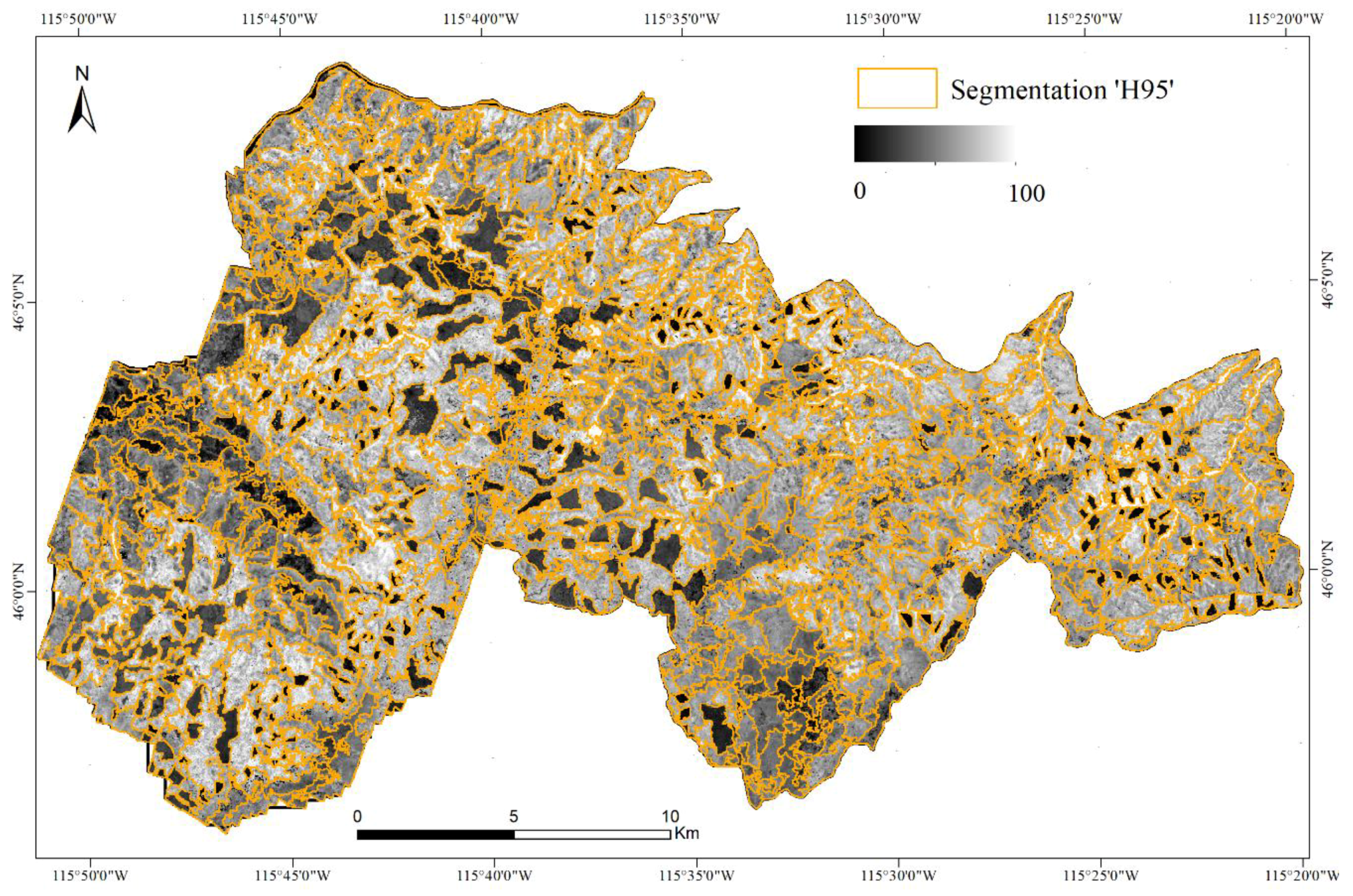
Figure 10.
Validation dataset: Reference objects delineated through visual interpretation of NAIP imagery and LiDAR point clouds (left); and corresponding image objects of the optimal segmentation of the ‘H95′ LiDAR metric (right). Even-aged forest stand (EAF) reference objects and their corresponding image objects are shown in green, and uneven-aged forest stand (UAF) reference objects and their corresponding image objects are shown in gray. A total of 100 reference objects were generated through visual interpretation of NAIP imagery and LiDAR point clouds: 25 EAF (average area: ~23 ha) and 25 UAF (average area: ~158 ha) on each LiDAR dataset.
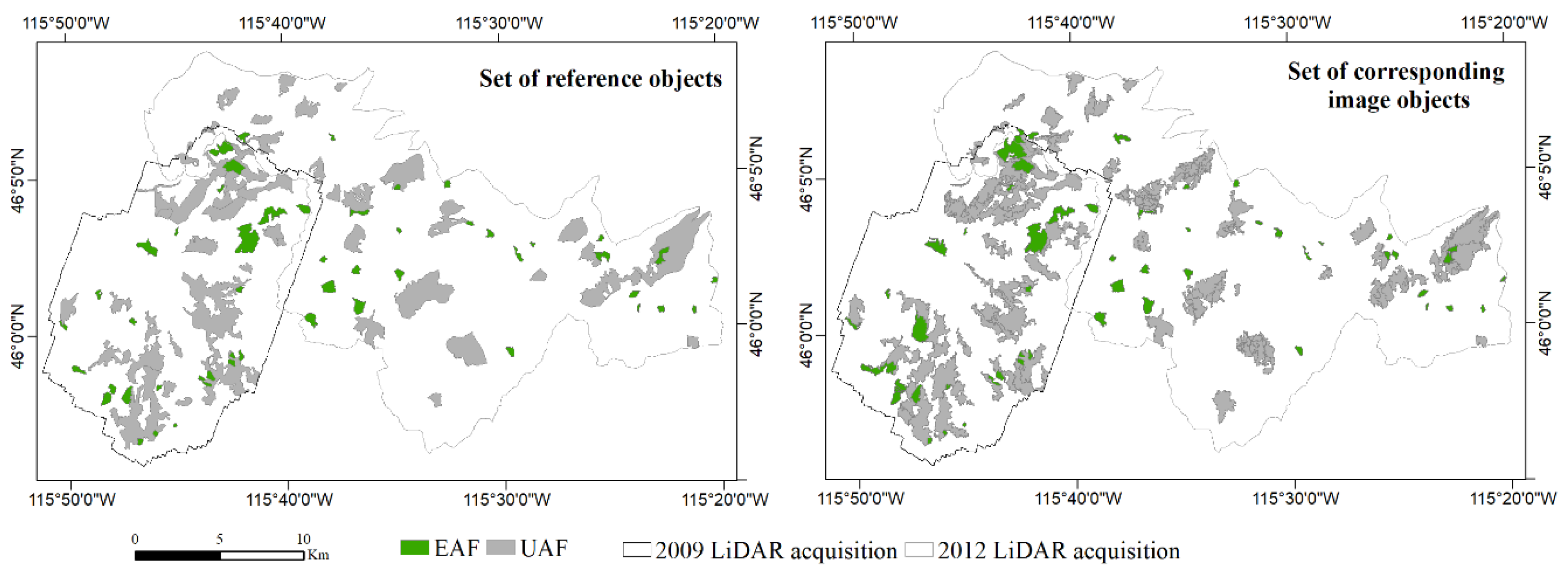
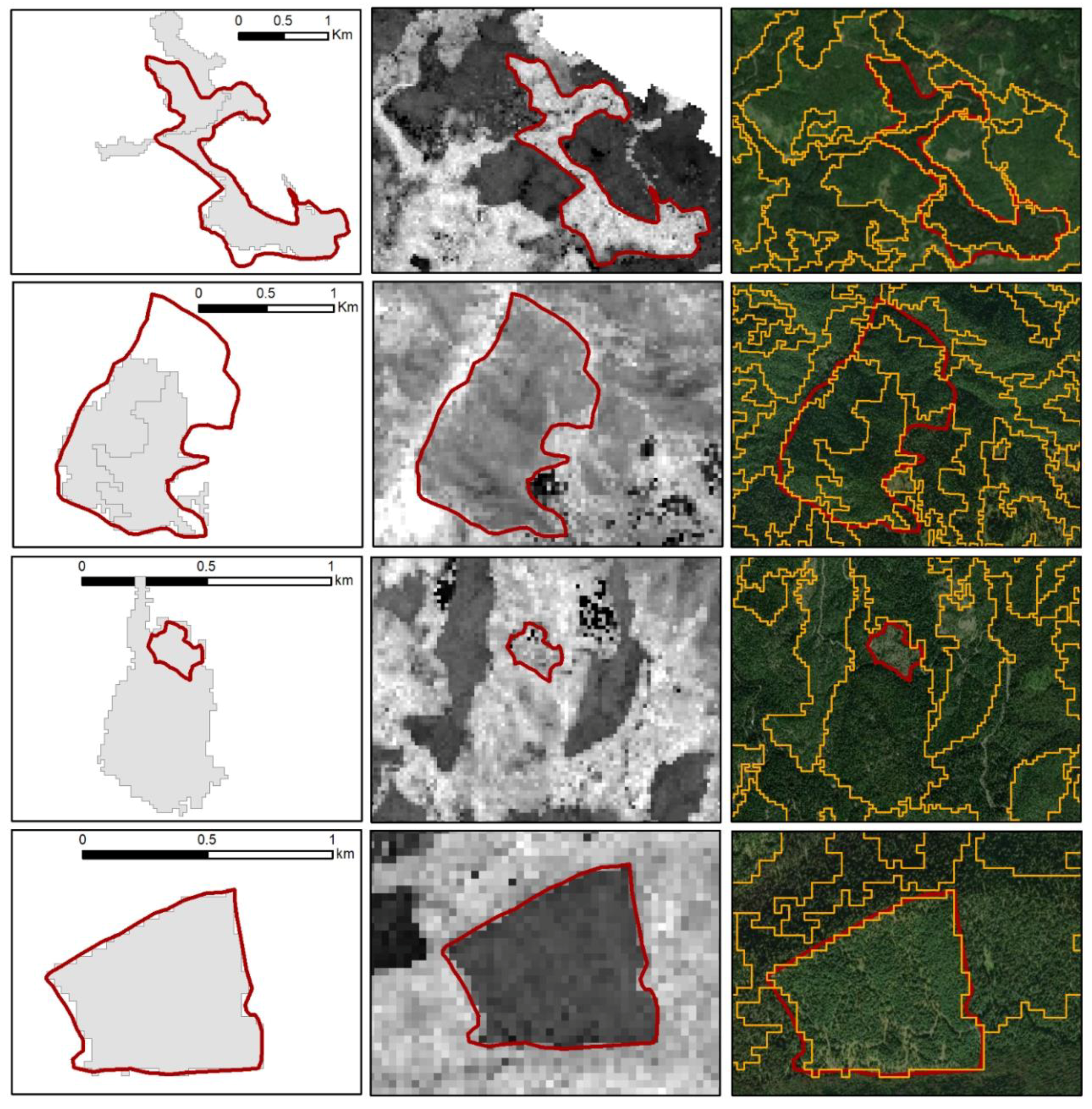
Figure 11.
Illustrative examples of the spatial relationship between visually interpreted reference objects and corresponding image objects of the optimal segmentation of the ‘H95′ LiDAR metric. The two top rows present examples of uneven-aged forest stands (UAF), and the two bottom rows present examples of even-aged forest stands (EAF). Left column: Reference objects (red polygons) and set of the corresponding image objects (gray polygons). Center column: Reference objects overlaid on the ‘H95′ LiDAR metric shown in grayscale. Right column: Reference object and all image objects (orange polygons) overlaid on 1 m spatial resolution NAIP imagery used to generate the validation dataset, shown in true color.


Table 1.
Light Detection and Ranging (LiDAR) summary metrics gridded at 30 m resolution from LiDAR point clouds. Twenty-five metrics are related to vegetation canopy height, and eleven are related to canopy density.
Table 1.
Light Detection and Ranging (LiDAR) summary metrics gridded at 30 m resolution from LiDAR point clouds. Twenty-five metrics are related to vegetation canopy height, and eleven are related to canopy density.
| LiDAR Metrics | Description | |
|---|---|---|
| Canopy height | ‘H01′ | 1th percentile of height above 1.37 m |
| ‘H05′ | 5th percentile of height above 1.37 m | |
| ‘H10′ | 10th percentile of height above 1.37 m | |
| ‘H20′ | 20th percentile of height above 1.37 m | |
| ‘H25′ | 25th percentile of height above 1.37 m | |
| ‘H30′ | 30th percentile of height above 1.37 m | |
| ‘H40′ | 40th percentile of height above 1.37 m | |
| ‘H50′ | 50th percentile of height above 1.37 m | |
| ‘H60′ | 60th percentile of height above 1.37 m | |
| ‘H70′ | 70th percentile of height above 1.37 m | |
| ‘H75′ | 75th percentile of height above 1.37 m | |
| ‘H80′ | 80th percentile of height above 1.37 m | |
| ‘H90′ | 90th percentile of height above 1.37 m | |
| ‘H95′ | 95th percentile of height above 1.37 m | |
| ‘H99′ | 99th percentile of height above 1.37 m | |
| ‘MaxH’ | Maximum height value | |
| ‘AveH’ | Mean height value | |
| ‘ModeH’ | Modal height value | |
| ‘VarH’ | Variance of heights | |
| ‘QMH’ | Quadratic mean of heights | |
| ‘SVH’ | Standard deviation of heights | |
| ‘CVH’ | Coefficient of variation of heights | |
| ‘Skew.H’ | Height skewness | |
| ‘IQH’ | Interquartile coefficient of heights | |
| ‘CRR’ | Canopy relief ratio | |
| Canopy density | ‘First returns above mean’ | Percentage of first returns above mean height over the total number of first returns |
| ‘First returns above 1.37 m’ | Percentage of first returns above 1.37 m height (breast height) over the total number of first returns | |
| ‘All returns above mean’ | Percentage of all returns above the mean height over the total number of returns | |
| ‘All returns above 1.37 m’ | Percentage of all returns above 1.37 m (breast height) over the total number of returns | |
| ‘Stratum below 0.15 m’ | Percentage of returns below 0.15 m | |
| ‘Stratum 0.15–1.37 m’ | Percentage of returns between 0.15 and 1.37 m | |
| ‘Stratum 1.37–5 m’ | Percentage of returns between 1.37 and 5 m | |
| ‘Stratum 5–10 m’ | Percentage of returns between 5 and 10 m | |
| ‘Stratum 10–20 m’ | Percentage of returns between10 and 20 m | |
| ‘Stratum 20–30 m’ | Percentage of returns between 20 and 30 m | |
| ‘Stratum above 30 m’ | Percentage of returns above 30 m |
Table 2.
LiDAR metrics considered in the analysis. The ‘H95′ and ‘Stratum above 30 m’ metrics were selected based on literature review. From the remaining 34 metrics, the five metrics with absolute average value of the Pearson’s correlation coefficient of the two LiDAR datasets (i.e., Clear Creek and Selway) lower than 0.5 (i.e., |R| < 0.5) with both ‘H95′ and ‘Stratum above 30 m’ were selected.
| Pearson’s Correlation Coefficient (R) | ||||||
|---|---|---|---|---|---|---|
| Clear Creek | Selway | Average | ||||
| LiDAR Metric | R(‘HP95′) | R(‘Stratum above 30 m’) | R(‘HP95′) | R(‘Stratum above 30 m’) | R(‘HP95′) | R(‘Stratum above 30 m’) |
| ‘HP95′ | - | 0.81 | - | 0.76 | - | 0.79 |
| ‘Stratum above 30 m’ | 0.81 | - | 0.76 | - | 0.79 | - |
| ‘CVH’ | 0.05 | −0.37 | −0.08 | −0.54 | −0.02 | −0.45 |
| ‘Stratum below 0.15 m’ | −0.26 | −0.37 | −0.36 | −0.43 | −0.31 | −0.4 |
| ‘Stratum 0.15–1.37 m’ | −0.28 | −0.28 | −0.27 | −0.55 | −0.28 | −0.41 |
| ‘Stratum 1.37–5 m’ | −0.20 | −0.23 | −0.28 | −0.50 | −0.24 | −0.36 |
| ‘Stratum 20–30 m’ | 0.02 | −0.02 | −0.05 | −0.06 | −0.01 | −0.04 |
Table 3.
Optimal segmentation of the seven considered LiDAR metrics. For each metric, the optimal set of multiresolution segmentation (MRS) algorithm parameters (scale, shape, compactness), the number of resulting image objects, and the unsupervised measures of spatial autocorrelation (normalized Moran’s I, normalized weighted Variance, modified Global score) are presented. The two LiDAR datasets were processed independently.
| LiDAR Metric | Scale | Shape | Comp. | # Image Objects | ||||
|---|---|---|---|---|---|---|---|---|
| Clear Creek | ‘H95′ | 29 | 0.1 | 0.1 | 347 | 0.47 | 0.23 | 0.37 |
| ‘CVH’ | 5 | 0.1 | 0.1 | 11,119 | 0.55 | 0.14 | 0.41 | |
| ‘Stratum below 0.15 m’ | 17 | 0.1 | 0.5 | 1295 | 0.56 | 0.24 | 0.43 | |
| ‘Stratum 0.15–1.37 m’ | 14 | 0.1 | 0.1 | 1131 | 0.57 | 0.24 | 0.43 | |
| ‘Stratum 1.37–5 m’ | 8 | 0.1 | 0.9 | 1495 | 0.58 | 0.24 | 0.44 | |
| ‘Stratum 20–30 m’ | 14 | 0.1 | 0.1 | 1439 | 0.55 | 0.25 | 0.43 | |
| ‘Stratum above 30 m’ | 59 | 0.1 | 0.1 | 151 | 0.39 | 0.35 | 0.37 | |
| Selway | ‘H95′ | 26 | 0.1 | 0.5 | 835 | 0.49 | 0.22 | 0.38 |
| ‘CVH’ | 5 | 0.1 | 0.1 | 16,592 | 0.57 | 0.14 | 0.42 | |
| ‘Stratum below 0.15 m’ | 20 | 0.1 | 0.1 | 994 | 0.59 | 0.25 | 0.46 | |
| ‘Stratum 0.15–1.37 m’ | 14 | 0.1 | 0.5 | 2112 | 0.55 | 0.26 | 0.43 | |
| ‘Stratum 1.37–5 m’ | 11 | 0.1 | 0.9 | 2585 | 0.54 | 0.26 | 0.42 | |
| ‘Stratum 20–30 m’ | 17 | 0.1 | 0.1 | 1915 | 0.54 | 0.28 | 0.43 | |
| ‘Stratum above 30 m’ | 23 | 0.1 | 0.1 | 1511 | 0.52 | 0.22 | 0.40 |
Table 4.
Supervised selection of the optimal LiDAR metric. Area-based dissimilarity metrics of oversegmentation (OS), undersegmentation (US), and summary score (D) are presented for the optimal segmentation of the seven considered LiDAR metrics; the number of reference objects with no corresponding image objects is also reported (Nnull). Four scenarios, based on the age of clearcut of the Forest Service Activity Track System (FACTs) harvest reference polygons, are considered: All clearcuts (1956–1996), clearcuts performed before the start of the Landsat MSS record (1956–1972), clearcuts performed before the start of the Landsat TM record (1956–1984), and clearcuts performed after the start of the Landsat TM/ETM+ record (1984–1996). For each scenario, the D score value of the optimal metric is marked (bold and underlined).
| All Clearcuts (1956–1996) | Pre Landsat (1956–1972) | Pre Landsat TM (1956–1984) | Landsat TM (1984–1996) | ||||||||||||||
|---|---|---|---|---|---|---|---|---|---|---|---|---|---|---|---|---|---|
| LiDAR Metric | Nnull | OS | US | D | Nnull | OS | US | D | Nnull | OS | US | D | Nnull | OS | US | D | |
| Clear Creek | ‘H95′ | 0 | 0.21 | 0.37 | 0.30 | 0 | 0.15 | 0.55 | 0.40 | 0 | 0.15 | 0.52 | 0.38 | 0 | 0.28 | 0.20 | 0.25 |
| ‘CVH’ | 0 | 0.86 | 0.16 | 0.62 | 0 | 0.81 | 0.19 | 0.59 | 0 | 0.82 | 0.18 | 0.60 | 0 | 0.90 | 0.14 | 0.64 | |
| ‘Stratum below 0.15 m’ | 12 | 0.53 | 0.47 | 0.50 | 4 | 0.55 | 0.52 | 0.53 | 5 | 0.55 | 0.51 | 0.53 | 7 | 0.52 | 0.43 | 0.48 | |
| ‘Stratum 0.15–1.37 m’ | 11 | 0.53 | 0.49 | 0.51 | 5 | 0.52 | 0.56 | 0.54 | 8 | 0.54 | 0.57 | 0.55 | 3 | 0.51 | 0.41 | 0.46 | |
| ‘Stratum 1.37–5 m’ | 8 | 0.44 | 0.52 | 0.48 | 4 | 0.46 | 0.56 | 0.51 | 6 | 0.47 | 0.56 | 0.52 | 2 | 0.40 | 0.47 | 0.43 | |
| ‘Stratum 20–30 m’ | 7 | 0.44 | 0.27 | 0.36 | 4 | 0.61 | 0.32 | 0.49 | 6 | 0.62 | 0.33 | 0.50 | 1 | 0.24 | 0.20 | 0.22 | |
| ‘Stratum above 30 m’ | 2 | 0.12 | 0.80 | 0.57 | 2 | 0.14 | 0.80 | 0.57 | 2 | 0.13 | 0.76 | 0.54 | 0 | 0.10 | 0.85 | 0.61 | |
| Selway | ‘H95′ | 0 | 0.22 | 0.21 | 0.22 | 0 | 0.13 | 0.32 | 0.24 | 0 | 0.16 | 0.29 | 0.24 | 0 | 0.28 | 0.14 | 0.22 |
| ‘CVH’ | 1 | 0.87 | 0.17 | 0.63 | 1 | 0.88 | 0.17 | 0.63 | 1 | 0.85 | 0.18 | 0.62 | 0 | 0.89 | 0.16 | 0.64 | |
| ‘Stratum below 0.15 m’ | 15 | 0.45 | 0.62 | 0.54 | 6 | 0.58 | 0.50 | 0.54 | 8 | 0.56 | 0.53 | 0.55 | 7 | 0.36 | 0.69 | 0.55 | |
| ‘Stratum 0.15–1.37 m’ | 9 | 0.44 | 0.46 | 0.45 | 1 | 0.54 | 0.45 | 0.50 | 4 | 0.52 | 0.49 | 0.51 | 5 | 0.37 | 0.43 | 0.40 | |
| ‘Stratum 1.37–5 m’ | 9 | 0.44 | 0.38 | 0.41 | 6 | 0.57 | 0.47 | 0.52 | 7 | 0.56 | 0.46 | 0.51 | 2 | 0.34 | 0.30 | 0.32 | |
| ‘Stratum 20–30 m’ | 4 | 0.39 | 0.28 | 0.34 | 0 | 0.62 | 0.19 | 0.46 | 4 | 0.56 | 0.28 | 0.45 | 0 | 0.23 | 0.28 | 0.26 | |
| ‘Stratum above 30 m’ | 1 | 0.19 | 0.31 | 0.26 | 1 | 0.17 | 0.35 | 0.28 | 1 | 0.19 | 0.33 | 0.27 | 0 | 0.19 | 0.29 | 0.24 | |
Table 5.
Area-based dissimilarity metrics calculated from the validation dataset presented in Figure 10: Oversegmentation (OS), undersegmentation (US), summary score (D), modified oversegmentation (), modified undersegmentation (), and summary score ().
Table 5.
Area-based dissimilarity metrics calculated from the validation dataset presented in Figure 10: Oversegmentation (OS), undersegmentation (US), summary score (D), modified oversegmentation (), modified undersegmentation (), and summary score ().
| Area | Stands | OS | US | D | |||
|---|---|---|---|---|---|---|---|
| Clear Creek | All | 0.25 | 0.26 | 0.26 | 0.18 | 0.27 | 0.23 |
| UAF | 0.39 | 0.35 | 0.37 | 0.24 | 0.37 | 0.31 | |
| EAF | 0.12 | 0.18 | 0.15 | 0.12 | 0.18 | 0.15 | |
| Selway | All | 0.36 | 0.15 | 0.27 | 0.21 | 0.14 | 0.18 |
| UAF | 0.50 | 0.21 | 0.39 | 0.22 | 0.21 | 0.21 | |
| EAF | 0.22 | 0.08 | 0.16 | 0.20 | 0.08 | 0.15 |
© 2018 by the authors. Licensee MDPI, Basel, Switzerland. This article is an open access article distributed under the terms and conditions of the Creative Commons Attribution (CC BY) license (http://creativecommons.org/licenses/by/4.0/).
Share and Cite
MDPI and ACS Style
Sanchez-Lopez, N.; Boschetti, L.; Hudak, A.T. Semi-Automated Delineation of Stands in an Even-Age Dominated Forest: A LiDAR-GEOBIA Two-Stage Evaluation Strategy. Remote Sens. 2018, 10, 1622. https://doi.org/10.3390/rs10101622
AMA Style
Sanchez-Lopez N, Boschetti L, Hudak AT. Semi-Automated Delineation of Stands in an Even-Age Dominated Forest: A LiDAR-GEOBIA Two-Stage Evaluation Strategy. Remote Sensing. 2018; 10(10):1622. https://doi.org/10.3390/rs10101622
Chicago/Turabian StyleSanchez-Lopez, Nuria, Luigi Boschetti, and Andrew T. Hudak. 2018. "Semi-Automated Delineation of Stands in an Even-Age Dominated Forest: A LiDAR-GEOBIA Two-Stage Evaluation Strategy" Remote Sensing 10, no. 10: 1622. https://doi.org/10.3390/rs10101622
Note that from the first issue of 2016, this journal uses article numbers instead of page numbers. See further details here.