Accuracy of Unmanned Aerial Vehicle (UAV) and SfM Photogrammetry Survey as a Function of the Number and Location of Ground Control Points Used

Abstract

The geometrical accuracy of georeferenced digital surface models (DTM) obtained from images captured by micro-UAVs and processed by using structure from motion (SfM) photogrammetry depends on several factors, including flight design, camera quality, camera calibration, SfM algorithms and georeferencing strategy. This paper focusses on the critical role of the number and location of ground control points (GCP) used during the georeferencing stage. A challenging case study involving an area of 1200+ ha, 100+ GCP and 2500+ photos was used. Three thousand, four hundred and sixty-five different combinations of control points were introduced in the bundle adjustment, whilst the accuracy of the model was evaluated using both control points and independent check points. The analysis demonstrates how much the accuracy improves as the number of GCP points increases, as well as the importance of an even distribution, how much the accuracy is overestimated when it is quantified only using control points rather than independent check points, and how the ground sample distance (GSD) of a project relates to the maximum accuracy that can be achieved.

1. Introduction

The possibility of taking pictures from small aerial unmanned vehicles combined with recent advances in computer vision and photogrammetry, now allow representations of the earth surface to be captured in a fast and economical way [1]. However, the geometric accuracy of such representations is rarely evaluated fully [2].

The accuracy of an unmanned aerial vehicle (UAV) survey is the result of many diverse variables, including flight design, camera image quality, camera modelling methodology, SfM algorithms and geo-referencing strategy. The flight design should include adequate forward and side laps, and maintain a constant altitude over the ground and a homogeneous coverage across the whole area. With this configuration, and by choosing a good-quality camera, the subsequent processing of images using modern structure from motion (SfM) photogrammetry is effective. Such techniques utilize highly tested mathematical and photogrammetric algorithms, which require few operator decisions beyond predominantly secondary tasks such as selecting an appropriate processing resolution or filters and simply identifying and marking appropriate ground control targets. Unlike these previous tasks, which can be mostly executed with a high degree of automation, the definition of the georeferencing strategy requires proper decisions.

Any 3D surface model normally obtained by SfM photogrammetry is initially captured in an arbitrary reference system. Geo-referencing involves transforming this initial arbitrary datum into a predefined coordinate reference system. This can be done either directly using known exterior orientations of photographs (“direct geo-referencing”) or by providing appropriate coordinates to points (ground control points or GCP) that are recognizable in the photographs (“indirect geo-referencing”).

Direct geo-referencing requires the measurement of the coordinates of the camera at the exact moment the picture is acquired, which is a challenge because the unmanned vehicle is moving, often with a velocity of several meters per second. With this movement, it is difficult to perfectly synchronize the camera triggering with the sampling frequency of the Global Navigation Satellite System (GNSS) receiver. If the integer ambiguities of the satellite and receiver ranges are not resolved, it is also obviously difficult to freeze the motion of the UAV in-flight whilst a GNSS solution is established. Finally, it is impossible to collect several epochs at each point to improve the position accuracy. Despite its convenience, this method of geo-referencing can therefore achieve only decimeter to meter accuracies, even for very high-resolution projects. For example, reference [1] obtained an accuracy of 1.247 m using imagery that had a resolution or ground sample distance (GSD) of 1 cm. Reference [2] reported an absolute modelling horizontal accuracy of 1.55 m and a vertical accuracy of 3.16 m. Reference [3] used a high-end inertial measurement unit (IMU) and GNSS receiver. This achieved vertical accuracies of 40 cm RMS using imagery with 0.7 cm GSD, which represents a relative accuracy (accuracy/GSD ratio) higher than 57. Reference [4] used a survey grade GNSS real-time kinematic (RTK) receiver (RTK UAV) and achieved similar horizontal accuracies when using GCP, but vertical accuracy errors were 2–3 times greater. They concluded that in applications requiring a vertical RMSE better than ±12 cm, GCP should be used rather than a GNSS/RTK platform. In [5], using a similar high-end RTK setup, authors state that without GCP the RMSE varies from flight to flight up to ±10 cm in elevation. Reference [6] also evaluated the performance of direct georeferencing with similar equipment. They achieved elevation discrepancies of about 4.7 GSD, but this was reduced to just 2.5 GSD when GCP were used. They concluded that it is unclear whether direct georeferencing (assisted aerial triangulation in their paper) will supersede GCP to become the standard referencing technique for UAV blocks.

Initial SfM 3D models can have deformations or systematic errors. Projective coupling or correlation between the inner and exterior orientation parameters leads to an inaccurate lens model and consequent model deformation. It has become recognized that processing vertical imagery with automated SfM procedures can generate an error surface in the form of a systematic dome feature [7,8,9,10,11]. These deformations can be reduced by using GCP [8,10,12]. If a simple conformal transformation without change in the shape of the SfM 3D model is applied, deformations will not be fully corrected since this only involves translating, rotating and applying the scale to minimize the image and ground residuals of coordinates of GCP. A second more complex approach is to reshape the 3D model by using the GCP information. This can include not only 3D transformations but also refinements of the geometric camera model (camera self-calibration) that also will change the relative position and orientation between cameras. Since the shape of the 3D model is allowed to deform, high confidence in the reliability and accuracy of the known coordinates is a requirement. This is only possible when enough time is dedicated to determinate the coordinates of GCP, normally through a rapid-static RTK survey. If inaccurate coordinates are introduced, instead of reducing the initial deformation, a more complex error surface will be introduced, which would be more difficult to isolate.

Evaluating the accuracy of a georeferenced 3D SfM can be done in different ways. A basic way involves analyzing the residuals from the bundle adjustment (BA) once the 3D model is rotated and scaled. As this method does not require nor use independent measurements, the measure should be analysed in terms of internal precision rather than accuracy. This method of evaluating the quality of a 3D model is not recommended, nor is it used in this paper. Our preference is to analyze the quality of a 3D model by using independently measured coordinates of ground points, which represent the “truth” to which the calculated photogrammetric coordinates of the model can be compared. Two approaches can be distinguished depending on whether the same control points are introduced as “ground control points” in the bundle adjustment (GCP-BA), or whether other independent points, named “ground check points”, are used. The most common option used by practitioners and non-specialist researchers is the first, as during the GCP-BA it is desirable to use as many points as available, as it is rather time-consuming and therefore expensive to establish control. However, evaluating the accuracy of a georeferenced model using control points is not fully objective, since the shape of the model adapts to the control points, and consequently GCP will always achieve the lowest residuals. Using check points provides a far more objective quantification of the true accuracy of geo-referencing procedures.

Another issue in terms of the georeferencing strategy using GCP is to determine how accuracy varies with the relative distribution of control, especially when few GCPs are available [13]. The general consensus in photogrammetry is to ensure that control is widely and uniformly distributed over the area covered by the images [14,15,16]. Unfortunately, there is no universal agreement about exactly what is best practice, and questions remain regarding whether GCP should be mainly located in the periphery, if it should occupy the center of the area, or what is the best general rule for placement.

The number of GCPs to use in a traditional aerial manned survey has been previously discussed in the photogrammetric literature. It is widely recognized that the more control points are used, the better the resulting accuracy is [16]. Nevertheless, the costs involved in establishing control points in large geographic areas forces a compromise to achieve appropriate accuracy with minimum operational costs [16]. Although these principles should be initially valid for UAV-based photogrammetry, this recent technology presents specific peculiarities with smaller sites and with the growing use of non-metric cameras and self-calibration for camera modelling. There is little published work concerning how the number of GCPs impact the accuracy of a UAV SfM survey, and many conclusions are either inconclusive or even contradictory. For example, reference [17] states that the number of GCPs used could be further decreased without significant loss of accuracy. Reference [13] uses different subsets of GCPs suggesting that the number of GCPs is an important parameters in accuracy results. Reference [18] analyses the accuracy of different setups using between 4 and 12 GCPs, with the authors concluding that the range of error decreased after using 7 or more GCPs. Reference [2] analyses results using between 3 and 22 GCPs. They recommend providing a high number of well-distributed GCPs to maximize accuracy, but they also state that with a minimum number of GCPs which are well distributed and with a high overlap, similar results can be obtained. Reference [8] concludes that the most accurate models were produced when using a higher number of GCPs. Reference [19] found that both horizontal and vertical accuracy improves as the number of GCP increases. They also find that in an 18-hectare (ha) SfM survey, 15 GCPs are necessary to achieve optimal results.

The main objective in the current research is to investigate empirically how the accuracy of a 3D SfM model varies with the location and number of control points used for geo-referencing. Analysis has been conducted to answer the followings questions: What is the best placement for the GCP? Is there a limit to model improvement? How many GCPs are needed to achieve a specific accuracy? How does this accuracy vary spatially both in plan and in height? How does the accuracy relate with the GSD? How should accuracies be compared using both control and check points?

2. Materials and Methods

2.1. The Aircraft

This study used a small 2 kg fixed-wing UAV plane, which was developed in-house and constructed from a light expanded polyolefin (EPO) foam body. This UAV is a simple flying wing design, equipped with two elevons as control surfaces and is typically used for UAV surveys over large areas. The aircraft has an endurance of 40 min with a cruise speed of 12 m/s. Most of the components, including servos, the motor, the electronic speed control unit and battery are standard industry parts. The positioning system of the plane used a coded-base single frequency L1, GPS, Glonass and WAAS U-Blox M8N GNSS receiver. This receiver was only used for aircraft navigation, and so its calculated position was not used during SfM processing or georeferencing. The flight controller on the aircraft is a Pixhawk autopilot, based on the open source Ardupilot and PX4 projects. This flight controller enables automatic flight during a mission consisting of waypoints or points of latitude, longitude and known height. The firmware programmed into the flight navigates the UAV through all waypoints using information provided by the inertial system, precision barometer, electronic compass and external GPS sensor.

Mission planning was done by the “Mission Planner” open source software [20]. With this software, the interest area is delimited, and by considering the internal geometry of the camera (sensor size and focal length), the desired flying height and the overlaps and waypoints of the photo flight are calculated. Once the mission is uploaded, the autopilot executes the flight fully automatically using the firmware, although the take-off and landing is still achieved through manual control.

2.2. The Camera

The UAV has a hole in the fuselage where a camera is housed. In this project, a Samsung NX500 camera with a Samsung NX 20 mm f/2.8 lens (W20NB) was used. This camera-lens assembly has an angular aperture of 60 degrees. The sensor of the camera utilizes a back-illuminated sensor (BSI-CMOS) technology with a size of 23.5 mm × 15.7 mm, with a maximum jpg resolution of 28 megapixels distributed in 6480 columns and 4320 rows. The longest side of the camera’s sensor was perpendicular to the direction of flight. The lens (Samsung NX 20 mm) is comprised of a simple and light (89 g) system of 6 elements in 4 groups. This lens does not have a zoom feature, so the movable elements are only those within the focusing group [21]. It has an electronic focusing ring, so the automatic focusing feature “Single AF” was used. The camera was connected to the autopilot controlling the location where the pictures were acquired.

A fixed exposure setting was used during the flight to ensure that each image achieved similar radiometry. Exposure time was fixed in 1/800 s. A medium aperture of f/4.5 was selected. The second lowest ISO sensor sensitivity (ISO 200) was sufficient to obtain good luminosity, both in shadow and bright areas. Other critical settings included white balance being fixed to daylight, the dynamic range feature being turned off, radial distortion camera correction being turned off and images being saved with the highest JPEG quality level. Raw data was not saved because detail loss in Super Fine JPEG quality is minimal. The exposure settings remained constant for all flights.

2.3. The Test Site

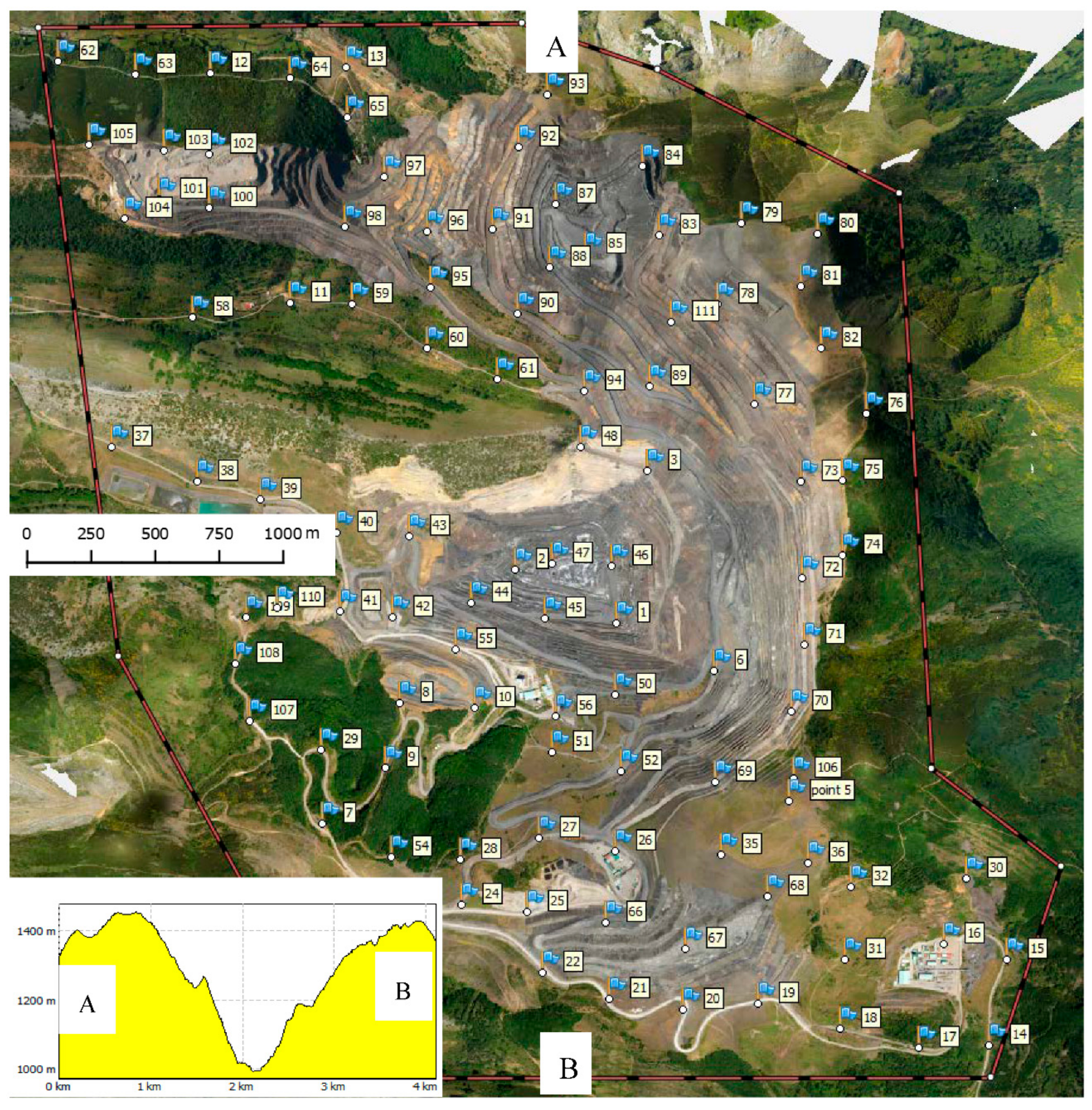
The flights were conducted in a highland and mining area located at the South of the Cordillera Cantábrica, near the village of Santa Lucia in León, Spain (Lat: 42°36′N; Long: 5°30′W). This is a coal mining area, which combines a small part of underground mining with large open cast exploitation (Figure 1). This environment is challenging for 3D modelling because of the low altitude of the flight in relation to the varying topography [22], which provides uniquely wide-ranging relief. The highest point of the study area has an elevation of 1548 m above sea level, while the lower part of the pit was below 990 m at the time the flight was performed. This represents a maximum elevation range of 558 m, with an average slope of 24.5 degrees. The test site is broadly rectangular, with approximate dimensions of 4 km × 3 km. In total, the area occupies 1225 ha.

2.4. The Flights

The flight control station was established at one of the highest points of the study area. The total area was divided into three parts: north, center and south. Two photo flights were carried out for each subzone: one in the E–W direction and another in the N–S direction. Each flight lasted approximately 40 min. Flights took place at a flight altitude of 1668, which is 120 m above the flight control station. As each strip was flown with a constant altitude, the varying topography caused a wide variation in flying heights above the ground. As a direct consequence, a wide range of GSDs was obtained, with an average GSD of 6.86 cm and a range between 3 cm and 11 cm.

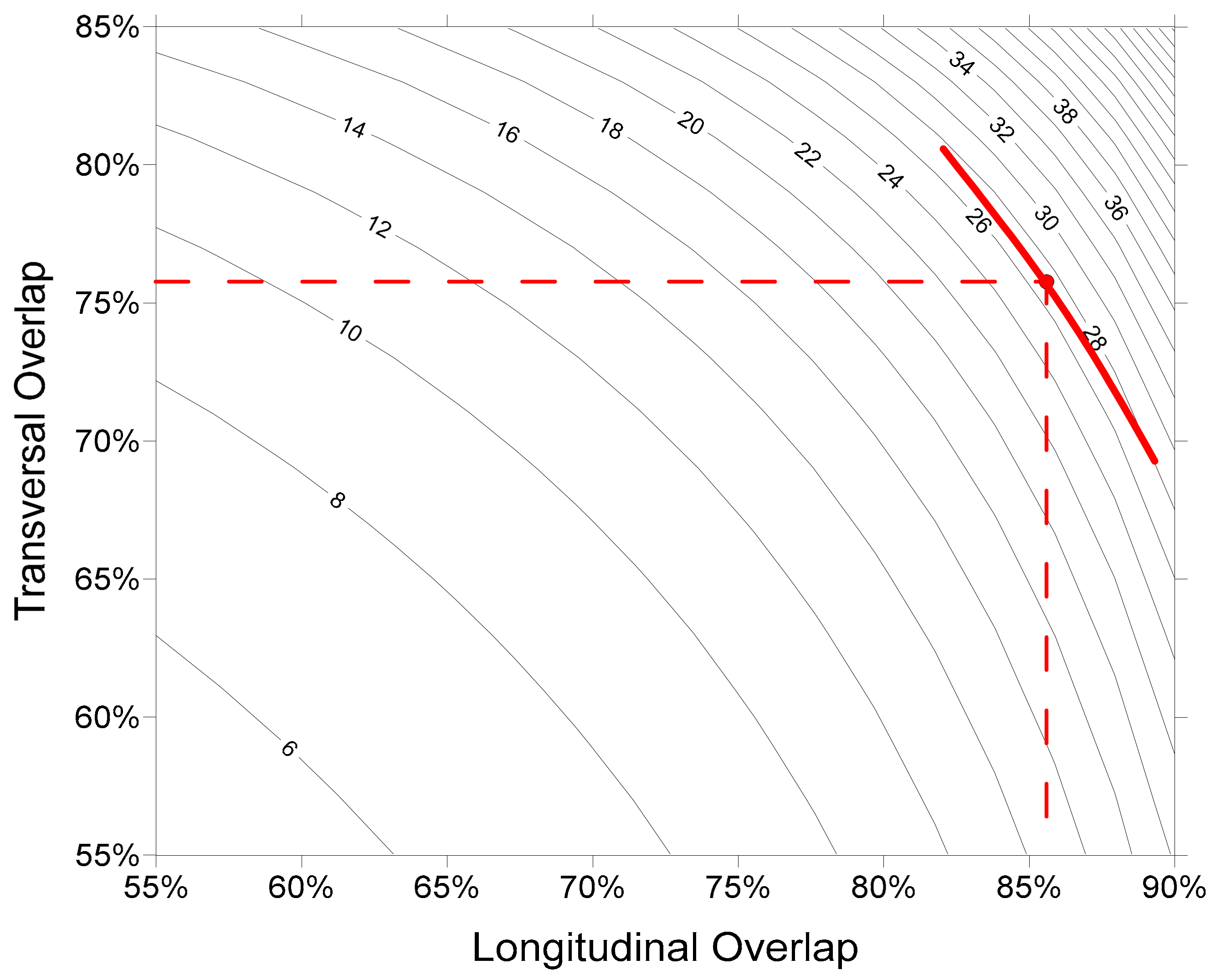
All flights in this project were planned with a 75% overlap and 60% sidelap, but the effective overlaps and side laps vary widely because of the large differences in height within strips and because two transverse flights were made within each subzone. The Agisoft PhotoScan Professional (APSP) software [23], used for all data processing, utilizes an “effective overlap index” (EOI) to describe image coverage redundancy. The images acquired for this project created an APSP EOI value of 12, but its calculation is not very well documented and therefore is only cited for reference and comparison. A more meaningful alternative synthetic overlap index (SOI) index can be calculated as the ratio between the imaged surface area and the real surface area, where the imaged surface area is calculated by multiplying the number of pictures by the image footprint at the mean project GSD. 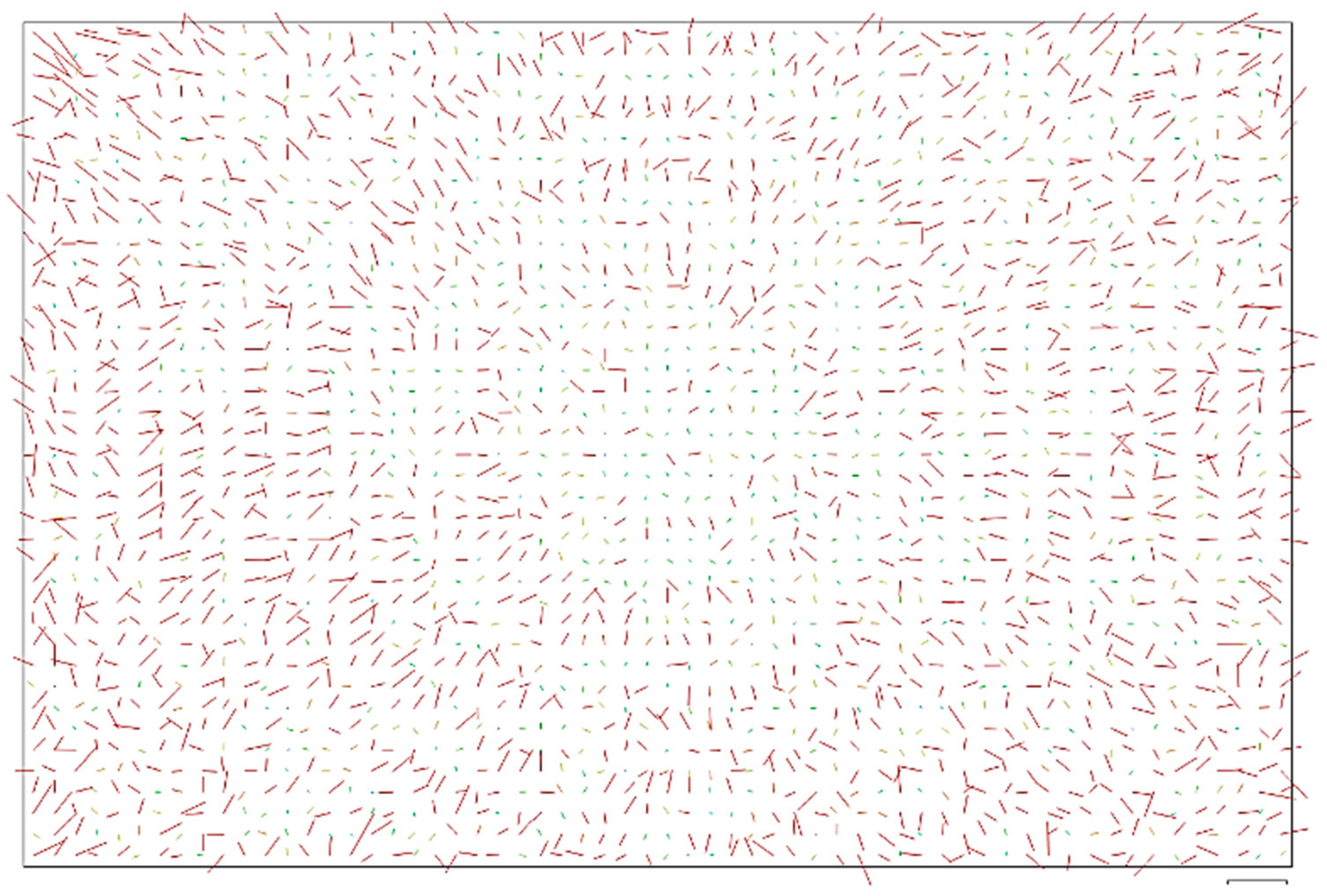Figure 2 shows the value of this EOI index (27), which would be equivalent to an average overall sidelap of 76% and overlap of 86%. During the six flights, a total of 2535 pictures were taken (Figure 3).

2.5. Obliquity of Imagery

A strong photogrammetric network should have two main features: highly redundant imagery and hence potentially highly redundant measurements, and diversity in camera roll angles, arranged in a strongly convergent imaging configuration [24]. Introducing oblique images in a perpendicular dataset allows larger angles between homologous rays that minimize systematic errors [25] or provide a better determination of internal geometry camera calibration, if appropriate parameters are introduced in the bundle adjustment. The UAV used in the flights uses just two elevons to control flight attitude, and so turns can only be achieved by rolling the plane. As a consequence, many images during the flight are not vertical. In this study, 50% of the total of 2514 images had an omega or phi angle greater than 10°, 20% of images had omega or phi angles greater than 20°, whereas 10% of images had angles greater than 25°. Omega, phi and kappa values were calculated and exported from the APSP software.

2.6. Ground Control Points

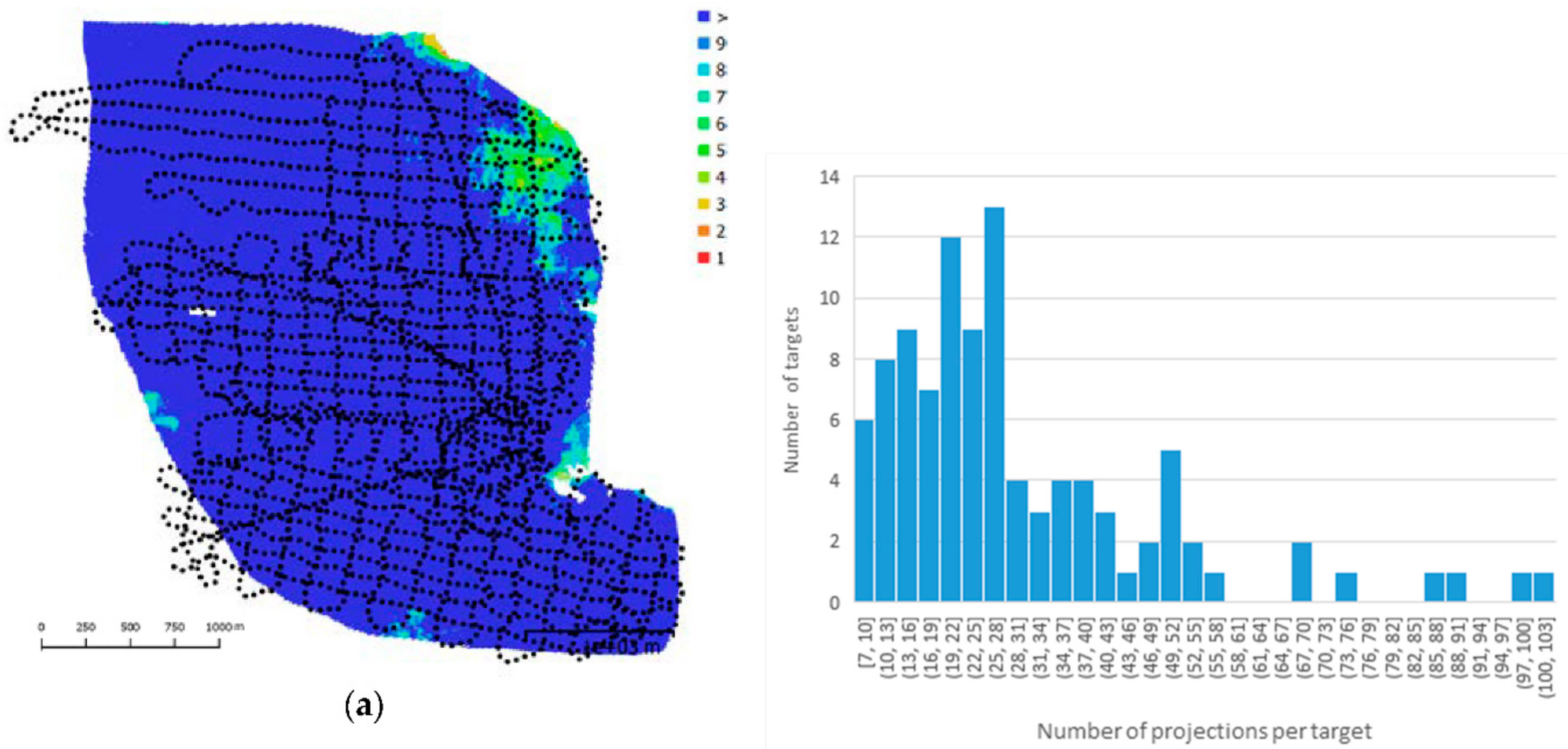
In classical photogrammetry, GCP must be distributed widely and uniformly throughout the whole block, particularly towards its periphery [14,16]. In UAV-SfM photogrammetry where non metric cameras are used, the best option is to try to distribute the GCP evenly or homogeneously in the periphery but also in the center of the area [2,8,26]. Consequently, 102 targets were placed evenly throughout the entire area before the flight. 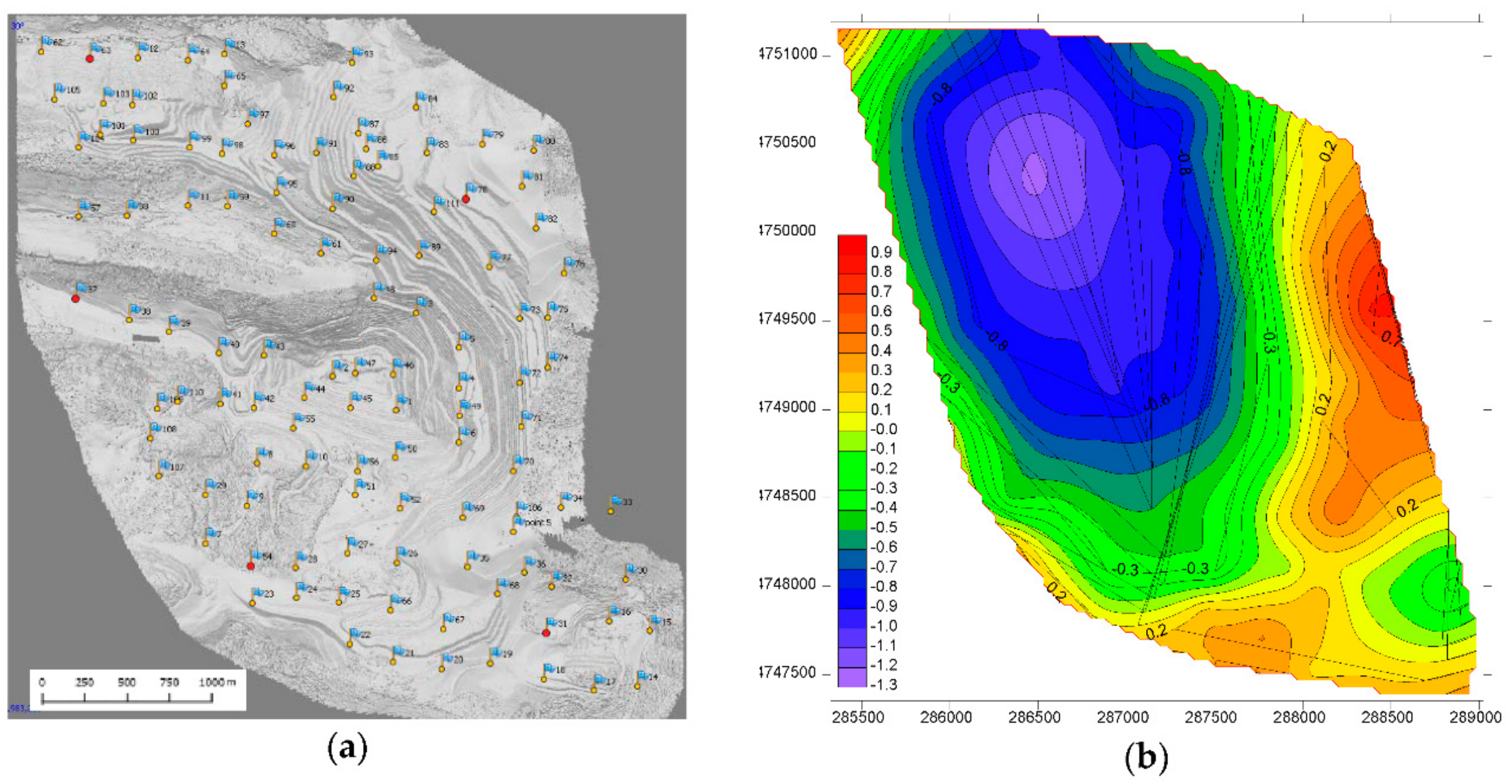Figure 1 shows the location of each GCP. Targets were created using 80 cm side squares of white and highly reflective material, which were fastened with nails and light-colored stones at the sides of roads, far from high vegetation, buildings or slopes. The coordinates of the targets were determined using a Javad Triumph-1 survey-grade GNSS receiver. At every target, 15 fixed epochs were averaged in RTK mode. A virtual reference station was used as established by the Red GNSS de Castilla y León, and corrections were received through an Internet stream. According to the manufacturer, the RTK performance of this receiver is 1 cm + 1 ppm × the distance to next reference station horizontally and 1.5 cm + 1 ppm × the distance to next reference station vertically, and so the expected accuracy of the coordinates was better than the GSD of the photos. Figure 1 shows the location of the GCP in relation to the study area.

SfM-UAV projects normally have a high imagery redundancy, and therefore, multiples views of the same scene from different view of points are expected. Figure 3b shows the number of images or projections in which one target appears. The average was 30.05 with a median of 24, close to the effective overlap index (27). Due to the wide-ranging relief, some of the targets (those in the middle of the working area and those at the lowest altitude) had more than 90 projections or views, while some peripheral and high-altitude targets had a minimum of eight projections (Figure 3).

2.7. Processing

Prior to photogrammetric data-processing, images were checked to eliminate blurred images which could compromise the initial image alignment [27]. The APSP software provides a tool called the “automatic image quality estimation feature” which generates an index based on the sharpness level of each image. Those generating low values were manually checked to distinguish if blur was apparent or if the image texture was homogenous. Any blurred images were removed and the remaining 2514 images were subsequently processed.

Although the same physical camera was used for the six flights, each set of images of a particular flight was treated individually, meaning that during data processing six different virtual cameras were used. This decision was judged to be prudent because the camera may have suffered some impact during each landing of the UAV and consequently the internal geometry could have changed [28].

Images were initially aligned or oriented in one Photoscan project, utilizing the medium accuracy option. Processing time was reduced by selecting the option “generic pair preselection”. With this option, a low-resolution image matching the alignment between all images is achieved initially. In a second step, image matching alignment is repeated at a higher resolution considering only overlapping images. In the alignment processing stage, an upper limit of 40,000 feature points and 4000 tie points per image was considered. Alignment required 8 h used 30 min of processing time, during which 98.85% of the images were successfully aligned. Finally, 1.75 million tie points were captured, with an averaged reprojection error of 1.7 pixels.

To achieve geo-referencing, all targets in all photos were measured manually, using a cross on the computer screen to locate the center of the target. With an average GSD of 6.86 cm, and targets 80 × 80 cm in size, these occupied approximately 10 by 10 pixels. Targets located at lower elevations appeared smaller and were more difficult to measure.

For all of the tests, the modelling of the camera internal geometry was achieved by self-calibration during the bundle adjustment. The self-calibrations used the sparse point cloud (1.75 million tie points) and, depending on the test, all or several of the GCPs. Estimates for focal length, principal point offset, four radial distortion coefficients, four tangential distortion coefficients, two affinity and non-orthogonality (skew) coefficients and the image width and heights were derived.

Table 1. Example of a camera calibration parameter set showing values, errors, value/error ratios and correlations. Correlations over 0.5 are in bold. (Source: Agisoft PhotoScan).

	Value	Error	Value/Error	f	Cx	Cy	B1	B2	K1	K2	K3	K4	P1	P2	P3	P4
f	5623.59	0.0921	61040.1	1.00	0.01	−0.05	0.10	0.01	−0.58	0.52	−0.48	0.44	0.02	0.02	−0.06	0.07
Cx	88.4463	0.0922	959.08		1.00	0.07	0.11	0.11	0.10	0.00	0.00	0.01	0.63	0.18	−0.16	0.11
Cy	54.9944	0.0673	816.65			1.00	−0.07	0.07	0.00	0.01	−0.01	0.02	0.19	0.65	−0.16	0.12
B1	1.83081	0.0166	109.94				1.00	0.02	0.07	−0.09	0.09	−0.07	0.05	−0.02	−0.02	0.03
B2	−0.2962	0.0169	−17.57					1.00	0.00	0.00	−0.01	0.01	0.03	0.02	−0.01	0.02
K1	−0.0112	2.6 × 10−4	−42.70						1.00	−0.98	0.93	−0.88	−0.06	−0.03	0.13	−0.14
K2	0.02738	2.1 × 10−3	12.93							1.00	−0.99	0.96	0.09	0.05	−0.16	0.18
K3	−0.0344	6.7 × 10−3	−5.14								1.00	−0.99	−0.12	−0.07	0.20	−0.22
K4	0.0175	7.2 × 10−3	2.44									1.00	0.14	0.09	−0.24	0.26
P1	2.95 × 10−3	1.3 × 10−5	225.42										1.00	0.09	−0.80	0.71
P2	1.50 × 10−3	7.4 × 10−6	202.58											1.00	−0.69	0.61
P3	−0.4290	0.021	−20.04												1.00	−0.98
P4	0.4150	0.0405	10.24													1.00

shows an example of a typical camera parameter set including errors and correlation. Despite the high degree of correlation between some pairs of parameters, which is expected due to the polynomic nature of the model [29], a fully flexible model was used since the value/error ratio in every parameter was generally higher than 1 or lower than −1.

Figure 4 shows a grid with all averaged residuals presented across the entire surface of the sensor with a magnification factor of 302. Some indicators of a successful and accurate camera self-calibration are demonstrated, which include (1) residuals sizes being homogenous (0.1–0.3 px) across the entire surface sensor, and (2) the concentric distribution of image residuals revealing that residuals comes from a limited polynomic model. In an inaccurate calibration, these concentric residuals are less conspicuous because in areas where the projective model does not match the actual behaviour of light paths, residuals are much larger.

2.8. Conducted Tests

The main objectives of this research were to assess how accuracy varies depending on the number and location of control points, how to compare accuracy indicators determined using control and check points, and how to determine the maximum accuracy achievable in a GCP-BA project in relation to the GSD. The data to draw conclusions from were generated using multiple combinations of control points, running the corresponding bundle adjustment (including camera non-linear refinement) and evaluating accuracy both in control and check points for each combination. A Python script (available in Supplementary Materials) was coded to automate the process of generating data. In this script, an increasing number of ground points was chosen randomly and assigned as control. In the first round, only 3 GCPs were chosen and the remaining 99 points were assigned as check points. This initial configuration was processed and the camera geometry determined. After the GCP-BA, the RMSE in the horizontal and vertical axes was calculated independently for both the control points and check points. Once the first round had been completed, a different set of 3 points was used to define the control, and the processing was repeated. A number of 35 repetitions was arbitrarily chosen. After 35 different combinations using 3 control points was achieved, a new cycle with a higher (i.e., 4) number of control points and lower number (i.e., 97) of check points was again processed 35 times. The script successively increased the number of control points adopted, until 101 ground points were used as control and only 1 as a check point. In total, 35 × 99 = 3465 different combinations of control points were tested.

3. Results

3.1. Control Point RMSE vs. Check Point RMSE

Figure 5 shows the root mean square error (RMSE) obtained during the 3465 tests. The x-axis represents the number of control or check points used during the bundle adjustment. The y-axis represents the RMSE in meters using a logarithmic scale 2 base. In the graphic area, each red point represents the mean RMSE calculated for all check points in one test, whereas each green point represents RMSE calculated for the control points. The blue line represents the average ground sample distance (GSD) of the imagery.

The accuracy in Figure 5 is computed as the root of the quadratic sum of the three spatial components. Figure 6 is equivalent to Figure 5 but quantifies accuracies aligned to the three axes: easting, northing and vertical. In order to maintain clarity, Figure 6 shows results from only 990 tests.

When RMSE is calculated for the control points, there is no difference between the three components, as the deformation of the model adapts to the control points using the same weight for the three axes. However, when RMSEs are calculated for the check points with the same combinations, a greater variation between the vertical and horizontal axes can be detected clearly.

As could be observed in Figure 5 and Figure 6, the RMSE measured for the control points remains much smaller than the RMSE achieved for the check points. Figure 7 shows the ratio between both RMSEs as a function of the number of images per GCP. This ratio can be considered as an overestimation of the accuracy of a SfM survey when measured only through RMSEs for control rather than check points. In the figure, in order to get a smoother trend, each point has been calculated averaging the RMSE from all 35 repetitions with the same number of GCPs. Figure 7 properly shows the necessity of considering errors evaluated on check points instead of GCP in order to have a reliable estimate of the real reconstruction accuracy.

3.2. Accuracy of GCP as a Function of the GSD

The photo flights were carried out in an area exhibiting a wide variation in relief and as a consequence of the fixed flying altitude, a range of GSDs were obtained (2.7 cm to 11 cm). The average GSD was 6.8 cm. In order to determine how the accuracy varies with GSD, the RMSE of all 102 GCPs are conveyed in Figure 8. During GSD estimation, camera and GCP altitudes were taken into account. As shown in the figure, residuals seem to grow linearly with the GSD. There is a high dispersion in data (R² = 0.273), but a Pearson coefficient of 0.52 indicates moderate correlation. The slope in the regression line is less than 0.5. Figure 8 (right) conveys the number of image projections with GSD. As expected, lower points generate more projections, but there is a dependency on GCP location, since peripheral GCPs tend to have fewer projections. The numerical results in the figures are only valid for this study since they are totally dependent on the relief and the spatial distribution of the GCPs. However, it is interesting to point out that, within a project, the accuracy of a point is not directly proportional to the GSD but the slope of the line is approximately 1/2. This could be explained by the higher number of image projections that have the farthest points.

3.3. Maximum Accuracy of a GCP-BA SfM Project vs. GSD

Figure 9 analyzes the achieved accuracy derived using ground check points as a function of the number of GCPs per 100 photos used during GCP-BA. The y-axis represents the accuracy achieved relative to the GSD, so that it can be more usefully used for comparing projects with different GSDs. The x-axis defines the number of GCPs per 100 photos. Each individual data point in the figure has been derived from the average of all 35 tests using the same number of GCPs. These figures demonstrate that a planimetric RMSE accuracy similar to ±GSD was achieved in our tests with approximately 2.5–3 GCPs per 100 photos. With more than 3 GCPs per 100 photos, horizontal accuracy does not improve in a sensible way. However, vertical accuracy always improves towards 1.5 × GSD, which was the maximum vertical accuracy achieved in our tests by using 4 GCPs per 100 photos. These results confirm a classical rule in photogrammetry that for accuracy reasons the number of vertical GCPs has to be higher than planar GCPs. It is also relevant that with fewer than 1 GCPs per 100 photos, accuracy values rapidly degrade. Finally, when very sparse GCPs were established, a horizontal RMSE higher than ±4 × GSD or vertical higher than ±5 × GSD was achieved.

3.4. Geometric Distribution of GCPs

GCPs were initially distributed evenly across the whole interest area (Figure 1), although a perfect regular grid was not possible to achieve because of constraints imposed by the mining area and changes of altitude of almost 1000 m. For the 3465 combinations tested, the selection of GCPs was random, but as every combination was saved, an analysis of the accuracy versus the location of GCPs could be conducted. Figure 10 shows the accuracy versus the averaged distance between GCPs (Figure 10a), the standard deviation of distances between GCPs (Figure 10b), and both variables together (Figure 10c). Averaged distances and standard deviations were calculated using all GCPs used in each combination. The Matlab script used to carry out the calculation and results is included in the Supplemental Materials for this paper.

As can be observed, optimum accuracies for check points was achieved when GCPs in a particular combination had average distances of approximately 1850 m with standard deviations of ±935 m. These values are very similar to those derived when statistics are calculated using all 102 GCPs. Averaged distances lower than 1850 relate to situations where the GCPs did not cover peripheral areas, whilst averaged distances higher than 1850 imply fewer points, but these were well distributed across the whole area. For the standard deviations, values lower than ±935 meant that points were preferably grouped in small areas, whilst higher values implied there were large gaps between GCPs. While it is not a surprise that maximum accuracy is achieved when almost every ground point is used as control, it can be observed that RMSE values degrade if points are limited in number, poorly distributed, or widely separated. Although optimum accuracies are achieved with values very close to 1850 m ± 935 m, there is a distinctive high accuracy area in Figure 10c that includes moderate lower average distances and standard deviation to moderate higher average distances and standard deviation values. Moderate low value regions could be seen as geometric distributions of GCPs where some peripheral points are not available, but the central area is evenly covered. Moderate higher values in both variables indicate geometric distributions with a medium number of GCPs which are evenly and well distributed across the whole area. When all areas are analyzed together, it can be concluded that good accuracies will be achieved when the available number of GCPs is both high and evenly distributed across the whole area, which is intuitive. Clearly, to concentrate GCPs in specific areas, leave large gaps or concentrating points either towards the periphery or the center appear to be poor strategies.

4. Discussion

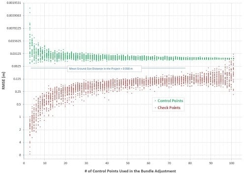
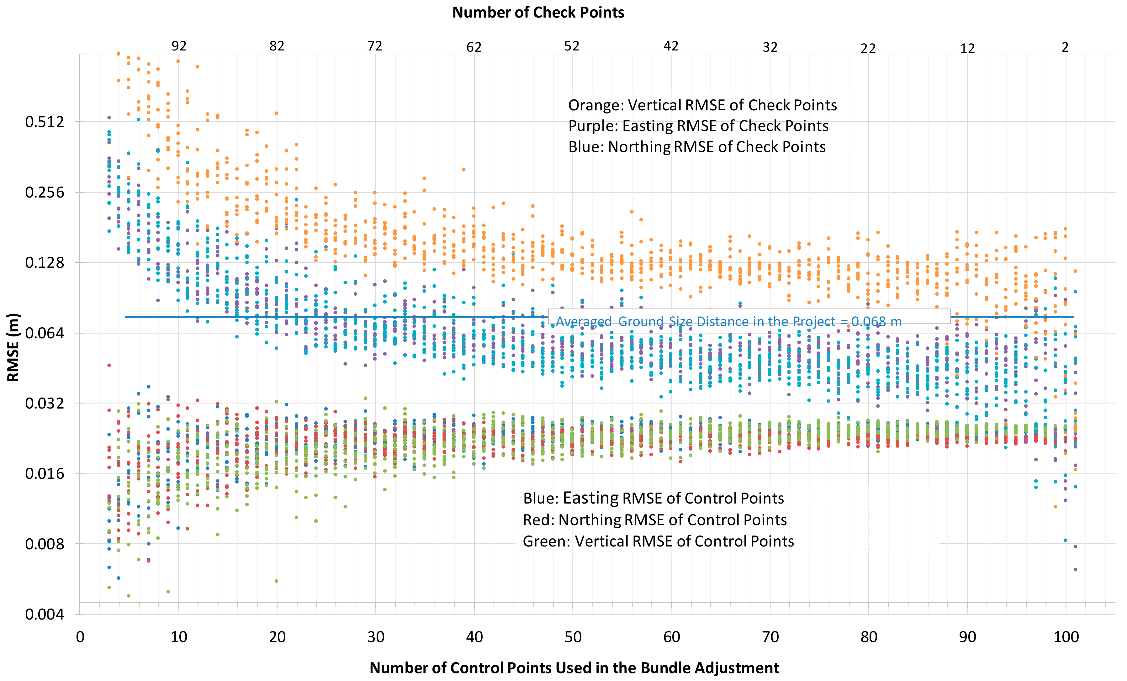
The geometric accuracy of an SfM photogrammetric 3D model is highly dependent on the ground georeferencing strategy, and the results of this study confirm that the accuracy is strongly dependent on the number of GCPs introduced in the bundle adjustment (BA). As illustrated by Figure 5, if few GCPs (10–20) are introduced into the BA, the RMSE in check points is over ±31 cm, roughly ±5 times the average GSD of the project. With 50–60 control points, the RMSE in check points improves to ±16 cm (±3 GSD). By introducing 90–100 control points, the RMSE in check points converges slowly to a value of ±12 cm, a value that is approximately double the average GSD of the project. These results largely agreed with those in [19]. It does not seem possible to improve this value further, regardless of the number of GCPs used. It is also interesting to note that according to expectations, those GCPs at low altitudes, and hence with higher GSDs due to the smaller photo scale, showed lower accuracy, although the loss of accuracy was half of that expected. A plausible reason for this is that more distant points appear on more images, hence achieving greater redundancy. This study has demonstrated also that optimum accuracies are achieved when GCPs are evenly distributed around the whole area. To concentrate GCPs in specific areas, to leave gaps without GCPs or to concentrate points on the periphery or in the center seem to be strategies that will not derive good accuracies. Ideally, GCPs should be distributed in a triangular node grid, since this distribution will minimize the maximum distance of any point to the nearest GCP.

When evaluating the geometric accuracy of an SfM 3D model, accuracy should not be measured using simply those ground points used as control in the GCP-BA. This is especially important if there are only a few GCPs. As can be observed in Figure 5, when only 3–5 points were used to provide control, the RMSE calculated at the control points was extremely low (sometimes just a few millimetres). However, the corresponding analysis using check points revealed that the real RMSEs of these projects were above ±1 m and even as high as ±8 m. With only a few GCPs, the deformation of the 3D model satisfies the few geometric restrictions introduced and consequently control residuals are extremely low.

It is not possible to correctly evaluate the geometric quality of an SfM 3D model using just a few check points, and indeed it can be perilous. To illustrate what occurs when just a few control points are introduced in the GCP-BA, a specific example is shown in Figure 11. Here, five control points were semi-randomly located towards the periphery of the working zone (Figure 11a). The RMSE error for these control points is very low (±0.03 m), which may be encouraging superficially, but Figure 11b illustrates large errors in heights obtained at the check points, with many greater than ±1.0 m. As the figure clearly shows, a systematic error surface is exhibited in the form of a “dome” feature, which has been often reported in SfM data processing [8,9,10,11]. It is important to note that this dome does not coincide with the mining pit, which occupies the center of the area, so is not related exactly to the site topography. The dome location, or where its height is maximum, is located as far as possible from all GCPs and of course does not obviously affect the control point RMSE. Depending on its location, the dome feature would not be detected if independent check points are located in the area between blue and green in Figure 11b. Consequently, a good evaluation of the geometric quality of an SfM 3D model should include many check points, which must be also evenly distributed across the whole area and not just located at the periphery. The continuous improvement of accuracy in the 3D model with an increasing number of control points is thus a consequence of a reduction of the dome size, probably through improved camera self-calibration in the BA.

The scatter of the RMSE clouds in Figure 5 must be related to the geometric distribution of the GCP in each project. A good geometrical distribution of GCPs will produce better accuracy and consequently lower RMSEs [2,8,26]. By observing the width of the check-point RMSE cloud in Figure 5 (red points) and assuming a high number of random geometries there will be both optimum and poor GCP configurations, it can be then observed that, for the same number of GCPs, the ratio between RMSEs will be around 2 between the best and worst check-point configurations. Thus, it can be deduced that the optimum geometry achieves half the RMSE of poor geometry for a similar number of points. Deriving a measure to define optimum geometry is outside the scope of this research, but possibly raises an important research question for the future.

With an increasing number of control points in the GCP-BA, the scatter of the RMSEs values measured in the same control points become reduced (green point cloud in Figure 5) and their values grow slightly to finally converge at around 4.1 cm, a value close to 2/3 the GSD of the project. This slight tendency for this RMSE to increase should not be interpreted as a deterioration of model georeferencing. The rigidity of the system is greater as more GCPs are used and the ability of a BA to adapt to all GCPs decreases. The lower scatter is easily explained as the more points there are available, the smoother the average is. In contrast, the degree of scatter for the check-point RMSEs (red point cloud in Figure 5) is not reduced and even increases for the final tests. This final higher variability in check-point RMSEs is because fewer check points remain in the tests as most of the points are being used for control. Consequently, the resulting RMSE averages are smoothed less.

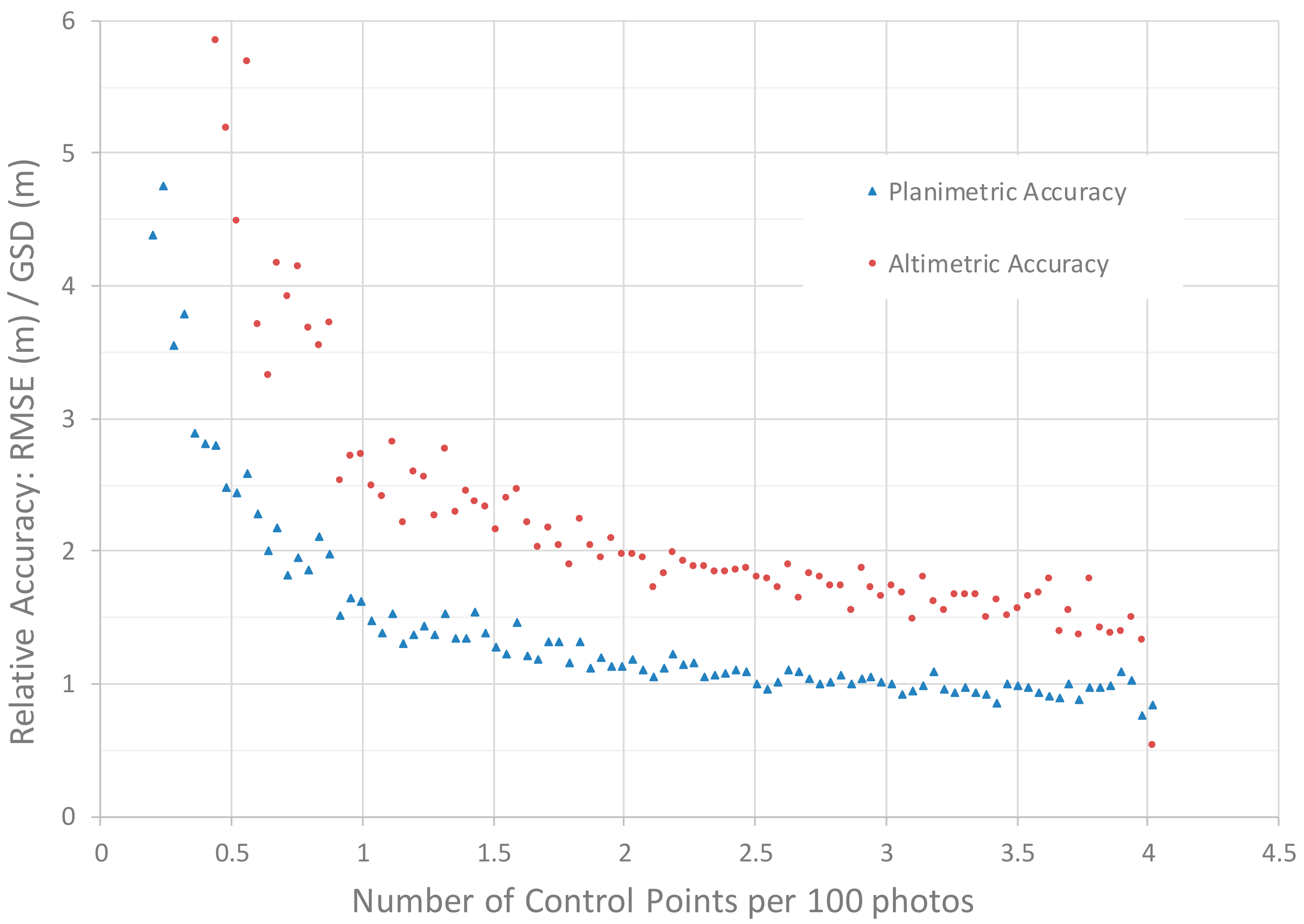
As illustrated by Figure 6, the accuracies of the horizontal and vertical components of am SfM photogrammetric 3D model are not the same. When accuracy is independently measured, vertical errors are 2.5 times the error of easting or northing. A broadly representative value for estimating the true height accuracy derived using a medium-optimum (50–60 in these tests) number of control points would be 2.3 times the GSD. By using a very high number of control points (90–100 in these tests), the height accuracy for the check points improves to 1.5 times the GSD. Planimetric accuracies are always better than GSD, including when a limited number of GCPs (20) are used. This planimetric accuracy continues improving when more points are added to converge to 0.66 × GSD. When RMSE is measured using just control (red, green and blue point clouds in Figure 6), the differences between vertical and horizontal components are not detected because GCP-BA adjusts the model equally to fit all 3 spatial directions. Consequently, if RMSE is measured using just control, horizontal accuracy will be underestimated and vertical accuracy will be overestimated.

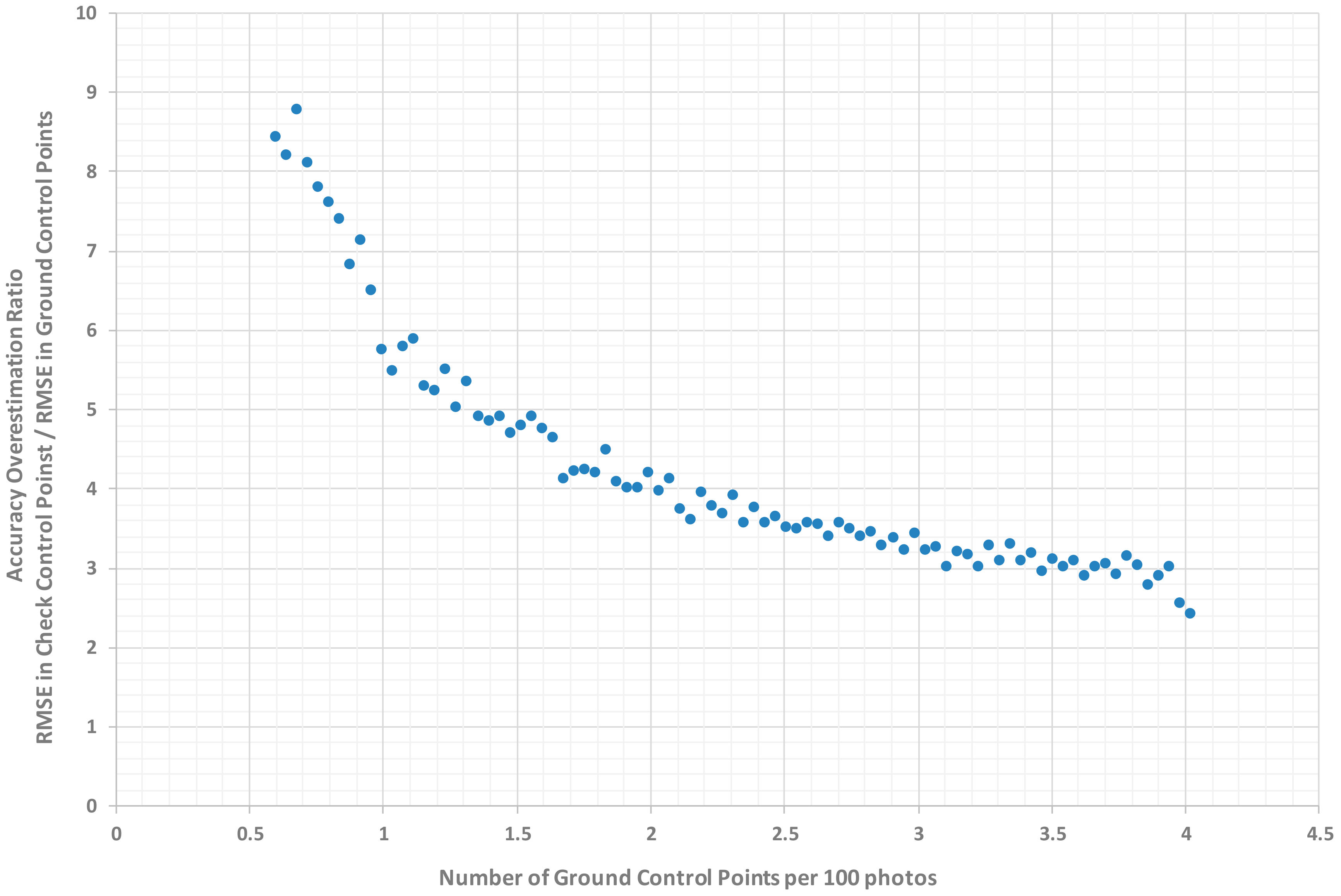
According to the first paragraph in this discussion section, the accuracy is improved by introducing all available ground points in the GCP-BA. In this situation, there will be no check points to evaluate correctly the accuracy of the resulting SfM 3D model, as recommended in the second paragraph. One possible solution is to introduce an “overestimation parameter” that relates control and check RMSEs as a function of the number of images per GCP (Figure 7). For example, for a project with a very high number of GCPs, the actual RMSE (measured using check points) could be estimated by multiplying the RMSE derived from GCP by an overestimation factor of 3. For projects with a medium number of GCPs, the overestimation factor would be around 4–5, whereas for a project with a medium to low number of GCP, the overestimation parameter would be 6. This approach is not recommended for projects with only a low number of GCPs. These ratios are calculated using the total RMSE in three dimensions. However, according to Figure 6, there are important differences between vertical and planimetric RMSEs derived using check points, so these overestimation ratios would be higher for vertical errors and lower for planimetric errors.

As can be observed in Figure 9, it is not possible to achieve a vertical accuracy that approaches the GSD, regardless of the number of GCPs used in a project. For plan accuracy, it is possible to achieve an accuracy similar to the GSD, providing there is at least one GCP for 35 images (this presumes that plan accuracy is the quadratic sum of the northing and easting errors). In practice, this represents a very high number of GCPs. With a more modest 50 images per GCP, a vertical accuracy of 2 × GSD and a 1.2 × GSD horizontal accuracy is achieved. With 75 images per GCP, accuracy worsens to 3 × GSD for vertical accuracy and 2 × GSD for horizontal accuracy.

It has been demonstrated that only with a medium to high number of GCPs can high accuracy ever be achieved. Here, high accuracy is achieved when the RMSE_3D is calculated at check points <±2 × GSD of the project. According to the recommendations made by other authors [8,10,11], some degree of convergent imagery was used in this work. Also, flight lines overlapped in opposing directions [10] and were acquired at a range of flying heights due to varying topography. Although findings in [12] confirm the need to have GCPs, our examination has been more exhaustive and demonstrates clearly that using just a few GCPs is unacceptable.

5. Conclusions

The work described in this paper has examined the geo-referencing and geometric quality of an SfM photogrammetric survey by computing accuracies using multiple combinations of GCPs. The study has been conducted using real data captured from a large project involving +2500 photographs and 102 ground points, covering an area of 1200 ha and exhibiting high relief. Although further studies using projects of different sizes, overlaps and image convergences would help to further generalize the results identified here, it is believed that the general trends found could extend to other UAV-based SfM projects. All accuracies have been therefore related to GSD to facilitate future comparison.

The results in this paper demonstrate how UAV-SfM photogrammetry accuracy depends on the location and number of GCPs introduced in the BA. If few GCPs are used, the RMSE in check points will be about ±5 times the averaged GSD of the project. By introducing a higher number of GCPs (more than 2 GCPs per 100 photos in our case study) the RMSE will converge slowly to a value approximately double the average GSD. These values are valid in 3D. As in classical photogrammetry, vertical errors in SfM photogrammetry will be 2.5 times the error of easting or northing components. The study has demonstrated that GCPs should be evenly distributed around the whole interest area, ideally in a triangular mesh grid, since with this setup the maximum distance to any GCP is minimized. Results indicate that for a given number of GCP, the accuracy achieved using an optimal distribution will be twice as good as that if GCPs are poorly distributed.

Accuracy should not be measured using the ground points used to control the BA. However, if independent check points are not available, real accuracy could be estimated by multiplying the 3D-RMSE derived from the GCP by a factor of 3 if the project has a high (more than 3.5 GCPs per 100 photos in our case study) or 4–8 if the project has a low number of GCPs (less than 2 GCPs per 100 photos).

Finally, it has been demonstrated that, in large projects, only with a medium to high number of GCPs (i.e., >3 GCP per 100 photos) can high accuracy be achieved. Even introducing oblique imagery into the vertical dataset or using high overlaps or crossed strips may not achieve high accuracy if just a few GCPs are used. There is no doubt that further research will reduce the ground point control dependence for large SfM projects. To use pre-calibrated cameras rather than the self-calibration approach, mixing different altitude flights, various degrees of image convergence, and using known positional and orientation parameters will all provide promising alternative opportunities in this quest.