Augmentation of Traditional Forest Inventory and Airborne Laser Scanning with Unmanned Aerial Systems and Photogrammetry for Forest Monitoring

Abstract

Forest inventories are constrained by resource-intensive fieldwork, while unmanned aerial systems (UASs) offer rapid, reliable, and replicable data collection and processing. This research leverages advancements in photogrammetry and market sensors and platforms to incorporate a UAS-based approach into existing forestry monitoring schemes. Digital imagery from a UAS was collected, photogrammetrically processed, and compared to in situ and aerial laser scanning (ALS)-derived plot tree counts and heights on a subsample of national forest plots in Oregon. UAS- and ALS-estimated tree counts agreed with each other (r² = 0.96) and with field data (ALS r² = 0.93, UAS r² = 0.84). UAS photogrammetry also reasonably approximated mean plot tree height achieved by the field inventory (r² = 0.82, RMSE = 2.92 m) and by ALS (r² = 0.97, RMSE = 1.04 m). The use of both nadir-oriented and oblique UAS imagery as well as the availability of ALS-derived terrain descriptions likely sustain a robust performance of our approach across classes of canopy cover and tree height. It is possible to draw similar conclusions from any of the methods, suggesting that the efficient and responsive UAS method can enhance field measurement and ALS in longitudinal inventories. Additionally, advancing UAS technology and photogrammetry allows diverse users access to forest data and integrates updated methodologies with traditional forest monitoring.

1. Introduction

Forest inventories are an integral component of natural resource monitoring and management. They provide the means needed to assess the health, growth, and disturbance regimes of forests and essential measurements for the estimation of biomass and productivity, both important ecological and economic indicators [1]. Moreover, they are an expected service of public agencies mandated to compile forest inventory data at the local, national, and global scales. The United States Forest Service maintains the database of the Forest Inventory and Analysis (FIA) Program—the largest system of permanent forest inventory plots in the world—annually with field enumeration [2]. The United Nations’ Food and Agriculture Organization (FAO), in part dedicated to tracking the state of the world’s forests, requests Forest Resource Assessments (FRA) from over 150 countries every five years [1]. Forest inventories typically involve in situ measurements at representative samples of dispersed plots. Frequency and spatial intensity of field surveys are often affected by financial constraints, resulting in infrequent inventories that often constitute a substantial undertaking and, occasionally, a burden for resource-strapped organizations. Accurate, timely, and economically acquired data would enhance improvements in present methodologies, support innovative monitoring schemes—in the manner of REDD+ [3,4]—and allow owners and managers of small forest holdings to leverage public data. Innovative methods to perform high spatial and temporal resolution data collection of forests while maintaining relevancy to existing data are needed [5].

Remote sensing is regarded as complementary or a potential alternative to ground-based inventories, offering high-resolution spatial information and temporal scales [6]. Three-dimensional (3D) remote sensing, in particular, is capable of capturing local, complex forest structure that is comparable to that of ground measurements and not available through two-dimensional products such as orthophotographs and satellite imagery [7]. Both active and passive remote sensing technologies including light detection and ranging (LiDAR) sensors and multiscopic photogrammetry can deliver 3D representations of forest stands. LiDAR instruments emit short pulses of light and measure the backscattered energy; differences in pulse return times and precisely recorded platform location and attitude yield 3D representations of targeted scenes. Airborne laser scanning (ALS) is broadly applied in forest monitoring, but its use is often limited, owing to steep acquisition and data-processing costs [8]. Conversely, digital photogrammetry is a technology that offers the capacity to map local forest inventory parameters in an affordable manner. Structure from motion (SfM) is a popular photogrammetric technique [9]. It derives three-dimensional scene abstraction, often called 3D reconstruction, in the form of a point cloud based on a collection of two-dimensional images exhibiting substantial overlap. By capitalizing on object representation redundancy across overlapping images, SfM accounts for perspective and image distortion effects and deduces, and once known, improves the accuracy of camera positions, a prerequisite for generating the scene point cloud. The recent proliferation of SfM-capable software, ranging from open source to commercial, has facilitated application to image collections [10]. These developments have made SfM ideally suited to light, inexpensive, yet high-resolution-imagery-capable cameras onboard recreational-grade unmanned aerial systems (UASs) and rendered it conducive to local forest monitoring and assessment. In contrast, typical laser scanning for forest inventory purposes is performed using manned aircraft or large UASs over much larger spatial scales and budgets [11,12].

SfM software advancements have been accompanied by increases in the sophistication and versatility of UAS hardware configurations, leading to consumer-friendly workflows [13]. Even recreational-grade UASs are now equipped with Global Positioning System (GPS) receivers, inertial measuring units, and internal positioning software that enable autonomous flight along predetermined trajectories [14,15]. Extraction of information from reconstructions via prescribed workflows is becoming more rote [16,17]. Derivatives directly comparable to ALS products include digital terrain (DTMs), canopy surface (DSMs), and canopy height (CHMs) models, along with individual tree detection (ITD) and crown delineations.

UASs are compact and easily transported. They can be flown at low above-target heights without concerns about cloud cover and employ low-impact technology. Small UASs can be deployed to landscapes ranging from hundreds of square meters to a square kilometer or more for rapid high-resolution data collection [7]. Unlike ALS acquisitions which typically require months of planning, a UAS acquisition can be completed within hours from the moment the decision is made or the need arises. These characteristics make UASs particularly suitable for private, nonindustrial forestland owners, replicable data collection, and studies of disturbance and growth. They have a wide range of applications [18], from monitoring deforestation [19] to capturing phenological dynamics in time series data [20]. The biggest driving forces behind UAS research in this context are the potential for inexpensive, expediated measurements and attainable quantitative assessments of change.

With the utility of small UAS-based photogrammetry for forest mensuration proven [21,22,23], focus is progressively shifting to the accuracy and precision of derived inventory parameters, including tree density estimates obtained by using ITD and crown delineation. ITD-based estimates of density explore the informational content of high-resolution imagery, have the same spatial data support (a single tree) as most national forest inventory protocols [21], tend to be more intuitive, and usually support and align to tactical management decisions better than estimates obtained using area-based methods. Early ITD approaches [24,25] continue to evolve, yielding improvements in performance, automation, and accessibility. The topic remains an active field of research [26,27,28,29].

Individual trees identified using a LiDAR- or UAS-photogrammetry-generated point cloud and furnished with an estimate of height support efforts to assess growth and competition rates, biomass levels, and other aspects of forest mensuration. Low cost and ease of deployment renders UAS-based photogrammetry compatible with the assessment of dynamic phenomena in short time increments [30]. Using panchromatic imagery from a total of four UAS flights within a period of six months, researchers succeeded in quantifying seasonal tree growth [31]. Under conducive conditions, patterns in SfM-predicted tree heights may also highlight limitations of standard or alternative measuring methods, such as bias in height assessment using field inventory techniques and LiDAR.

This study compares in situ forest inventory measurements to cotemporal, ALS-based measurements and also to photogrammetry derived equivalents from UAS imagery acquired two years later at a set of field plots participating in the Forest Service Carbon Monitoring System (CMS). The asynchronous data sources are evaluated for their potential to create a low-cost retrospective and cohesive monitoring scheme for forest plots. We are motivated to (i) provide a low-cost, user-friendly workflow for forest data collection via a small-UAS and consumer photogrammetry products; (ii) leverage similarities between ALS and digital imagery postprocessing to suggest small-UAS-derived photogrammetry as a preeminent tool to describe and augment existing forest inventories; and (iii) demonstrate how consumer UAS remote sensing can be integrated into the legacy of forest monitoring.

2. Materials and Methods

2.1. Forest Inventory and ALS Data

This study was conducted on plots enrolled in the Carbon Monitoring System (CMS) in Oregon. With the expressed purpose of developing a sampling design for longitudinal carbon quantification, the program acquired high-density LiDAR data and in situ measurements at representative plots in Oregon, Colorado, South Carolina, Maine, Minnesota, New Jersey, and Pennsylvania. Circular plots were established with a radius of 16.2 m, and an area of 824.5 m², or approximately one-fifth acre. Established plots were stratified in classes of canopy cover and tree height using LiDAR-derived metrics according to the procedure described in [32].

Airborne LiDAR data were acquired in the summer of 2015. Acquisition specifications are shown in

Table 1. 2015 light detection and ranging (LiDAR) acquisition specifications.

Parameter	Value
Scanner	Reigl 680i
Mirror	Rotating
Field of view	±30 degrees
Flying height	730 m (2400 ft) aboveground level
Pulse rate	330,000 Hz
Scan rate	200 Hz
Beam divergence	≤0.5 mrad
Pulse wavelength	Near infrared, 1064 nm
Intensity	16-bit
Processing	Digitized waveform, up to 7 returns per pulse in the study area

. The data vendor provided a 0.914 m (3 ft) LiDAR-derived Digital TerrainModel (DTM). A DSM registered to the DTM was created by assigning to each cell the 90th percentile elevation value of corresponding above ground returns.

Field data were collected in the fall of 2015 following the FIA protocol [33] that was modified to accommodate differences in plot footprint. The center of the plot was established with a survey-grade Javad Triumpth 1M rover (Javad Corporation, San Jose, CA, USA), reportedly capable of delivering submeter horizontal location precision under canopy conditions [34]. The project used the NAD83 (2011) projected coordinate system in UTM zone 10N and vertical datum NAVD88 based on the 12A geoid. The field crew tallied all trees within 4.6 m from the plot center but only those with a diameter-at-breast-height (DBH) greater than or equal to 12.7 cm on the full 16.2-m radius plot. To leverage a larger plot area, our analyses excluded trees with DBH smaller than 12.7 cm. Tree DBH was measured with tape at 1.37 m from the ground and tree height with a laser rangefinder.

2.2. UAS-Based Photogrammetry Data

We collected imagery data using a small-UAS in the summer and fall of 2017, approximately two years after the LiDAR and field data collection campaigns, over 11 CMS plots. The selected plots were evenly distributed over canopy cover and tree height classes (

Table 2. Characteristics of sampled field plots.

Canopy Cover Class (Percent)	Number of Plots	Number of Trees on Plot with DBH >= 12.7 cm	Maximum Tree Height (m)	Dominant Species (Number of Plots)
I (10–40%)	4	6–12	15.5–35.7	Ponderosa pine (3); Lodgepole pine (1)
II (40–70%)	4	9–19	9.4–43.9	Ponderosa pine (2); Lodgepole pine (2)
III (70–100%)	3	37–73	16.8– 28.3	Ponderosa pine (2); Lodgepole pine (1)

) and are representative of the biome’s population and forest conditions. Figure 1 shows the geographic distribution of the plots. Dominant species were ponderosa pine (Pinus ponderosa) and lodgepole pine (Pinus contorta). All plots were located on flat areas or modest slopes, under 6 degrees, or about 10 percent.

The UAS consisted of a 3D Robotics Solo outfitted with a gimbal and a GoPro Hero 4 Silver camera. The camera recorded a mid-range field of view at 3000 × 2250 pixel resolution and acquired a red, green, blue (RGB) image every 0.5 s during a cross-grid flight trajectory with 90% front overlap and 90% side overlap. The camera was nadir-oriented during the first flight pass and at 25 degrees from vertical during the perpendicular flight line. We chose to include angled views of the plots because oblique imagery improves variability in viewing geometry and enhances the representation of lower canopy components [35,36]. To control for edge effects, flight lines were extended by 50%, or an additional 16.2 m. Nominal flying altitude was set to 20 m above the tallest tree, notwithstanding changes in topography. Pre-deployment flight planning was done in Mission Planner [14] and implemented autonomously on-site with Tower, a mobile application [15]. Depending on the flying altitude, the UAS was airborne for 4–6 min and required 190–340 images to cover the scene. The resulting mean ground sampling distance was approximately 3 cm.

The location and altitude of the UAS during flight recorded by internal GPS and inertial navigation sensors were transcribed to the images by synchronizing the camera’s internal clock to that of the UAS and flight logging software and specifying the null differential during processing. To ensure precise georeferencing of the point clouds generated via photogrammetric processing, we placed at the center of each plot and at each approximate cardinal direction towards the plot boundary orange 18.9-liter (5-gallon) buckets that served as ground control references or points (GCPs). The coordinates for each marker center were derived using azimuth from true-north recorded with a compass and slope distance from the plot center using tape. The slope distance was later converted to horizontal using the LiDAR-derived DTM as reference. UAS imagery of forested scenes always has weak positional geometry, in the sense that all objects are viewed from a fairly narrow angular perspective. The combination of weak geometry and the presence of many inexact and homogenous features with similar neighbors and background induce distortions in scene scale and orientation [37]. Markers, each identifiable on a subset of the acquired images, ensured that these distortions were minimal.

A DSM was computed from the overlapping and multiperspective images using the photogrammetric workflow implemented in Agisoft Photoscan Professional version 1.4.2 [16]. The software generates an initial object 3D structure by identifying unique and invariant features across congruous images. Using the bundle adjustment algorithm, it establishes camera perspectives and accounts for the fish-eye lens characteristic of the GoPro [38]. Image alignment was conducted with “high” accuracy and generic preselection enabled, an option designed to speed up the computational time of image matching. Key point and tie point limits were set to 60,000 and 4000, respectively. Geotagged images improved the processing load during alignment by providing initial, approximate camera locations but were disabled in favor of GCP positions for subsequent processing in order to ensure precise orientation and scale. Each image was visually assessed and any unobscured GCP was identified and assigned its respective xyz coordinates, followed by an automatic camera alignment adjustment. At the end of this processing phase, a correctly oriented and scaled sparse point cloud of the scene was obtained. From the sparse point cloud and related scene positions, depth maps representing the distances between features and respective camera location were created for each image and combined into a comprehensive 3D reconstruction known as the dense point cloud. “Mild” depth filtering was specified for our scenes, a setting known to permit a limited number of outlier points yet maintains small, spatially distinguished details into the model. A “high” quality setting was determined as an acceptable compromise between accuracy and computational time, supported by recent evidence that it consistently yields optimal results when applied to scenes dominated by trees. Unlike other settings, the one selected directs Photoscan to operate on the full resolution of the original images. Conversely, the “highest” quality setting was found prone to serious degradations in point cloud accuracy and completeness, despite its substantially higher computational cost [10]. The final point cloud was exported in LAS format.

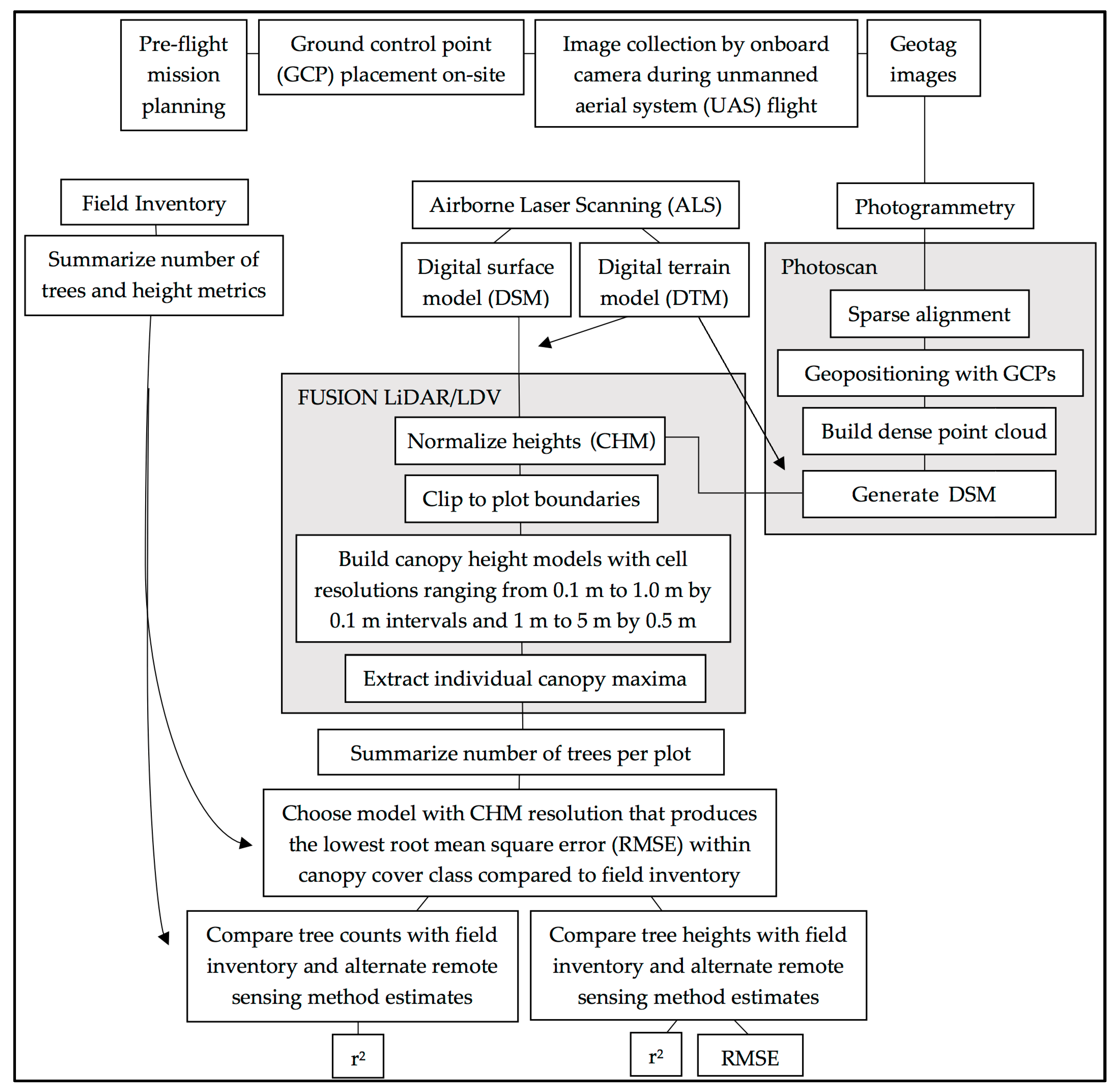
2.3. Point Cloud Postprocessing

We processed the LiDAR- and UAS-derived point clouds to extract individual tree measurements using FUSION LiDAR/LDV [39], which is publicly available software specializing in visualization and analysis of three-dimensional data. Of the various ways to perform ITD, the one implemented in FUSION employs a local maxima-based filtering approach applied using a user-specified window size on derived CHMs [39]. Each point cloud is clipped to the boundary of the area of interest—in our case, the CMS plot—and is normalized using the ALS-derived DTM before being processed by the CanopyModel module to generate the CHM. The CanopyModel assigns the aboveground value of the highest point within the planar area of each grid cell to the grid cell center. If requested by the user, it smooths the generated surface using a median or a mean filter or both while preserving local maxima. The resolution specified in the CanopyModel module is a key parameter critical for all ensuing analyses [40,41]. It could lead to ITD errors of commission if too fine and errors of omission if too coarse. In this study, we considered progressively coarser resolutions for the plot CHMs ranging from 0.1 to 1.0 by 0.1 m intervals and 1 to 5 by 0.5 m intervals for each of the three cover classes.

Next, we applied FUSION’s CanopyMaxima module. The module uses the CHM generated by the CanopyModel to identify local maxima using a variable-size window, sometimes referred to as a circular kernel of dynamic radius. The window size is calculated proportionally to the height of the CHM at the center of the window (kernel). The diameter D of the kernel centered at a CHM cell of value h was computed as

$$\mathrm{D}=0.681{\left[\frac{-1}{{\mathrm{P}}_3}\ln (\frac{\frac{\mathrm{h}}{0.3048}-4.5}{{\mathrm{P}}_2})\right]}^{\frac{{\mathrm{a}}_2}{{\mathrm{P}}_4}}$$

(1)

where D and h are expressed in meters with coefficient values P₂ = 1180, P₃ = 6.7, P₄ = −0.315, and a₂ = 0.82 derived from the Westside Cascades variant of the Forest Vegetation Simulator [42], as revised in 2017, for mixed pines.

We compared the number of plot trees identified by using progressively coarser CHM cell resolutions as shown above to those observed during the field visits. The root-mean-square error (RMSE) was used to quantify the canopy class-specific discrepancy for each CHM parameter setting as

$$MSE=\sqrt{{{\displaystyle \sum }}_{i=1}^N\frac{{\left(x_{if}-x_{ir}\right)}^2}{N}}$$

(2)

where N is the number of plots in the canopy class, x_if is the number of trees observed in the field, and x_ir is the number of trees extracted from the canopy height models. The cell resolution yielding the smallest RMSE was chosen as the optimal setting for the canopy class and was subsequently used in ITD.

We imposed a 7.73-m height threshold for identified trees to account for the DBH minimum that trees would have had to meet or exceed to be tallied according to the field protocol. The height threshold was calculated from a derivation of Equation (1) that relates the estimated height (in meters) of Westside Cascades variant mixed pines to DBH (in inches).

$$h=0.3048\left[e^{-P_3\times DB{H}^{P_4}}\times P_2+4.5\right]$$

(3)

We estimated the nominal height of plot trees with DBH of 12.7 cm (5 in) and included all trees with a height above this threshold in our 3D representations as discrete trees. We evaluated composite plot summaries based on estimates of tree count and height metrics (minimum, mean, and maximum). Performance was assessed by comparing these composite summaries across field-observed, UAS-, and ALS-based methods. The differences in CHM resolutions, tree counts, and tree heights were analyzed descriptively. The coefficient of determination of a linear correlation (r-squared) between methods was given for the comparison of tree counts and mean tree height as

$$r^2=cor\left(q_{ir},q_{if}\right){}^2$$

(4)

where q_ir equals the variable extracted from either the UAS or ALS point cloud, q_if equals the variable observed in the field, and i refers to one of the 11 plots. The RMSE for the difference in mean tree height among the methods was calculated as in Equation (2). Figure 2 presents a summary of our methodology in the form of a flowchart.

3. Results

3.1. Reconstructions

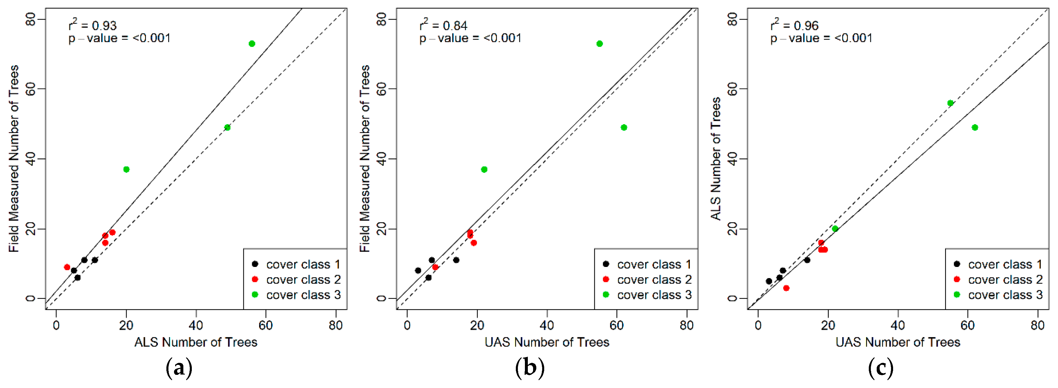
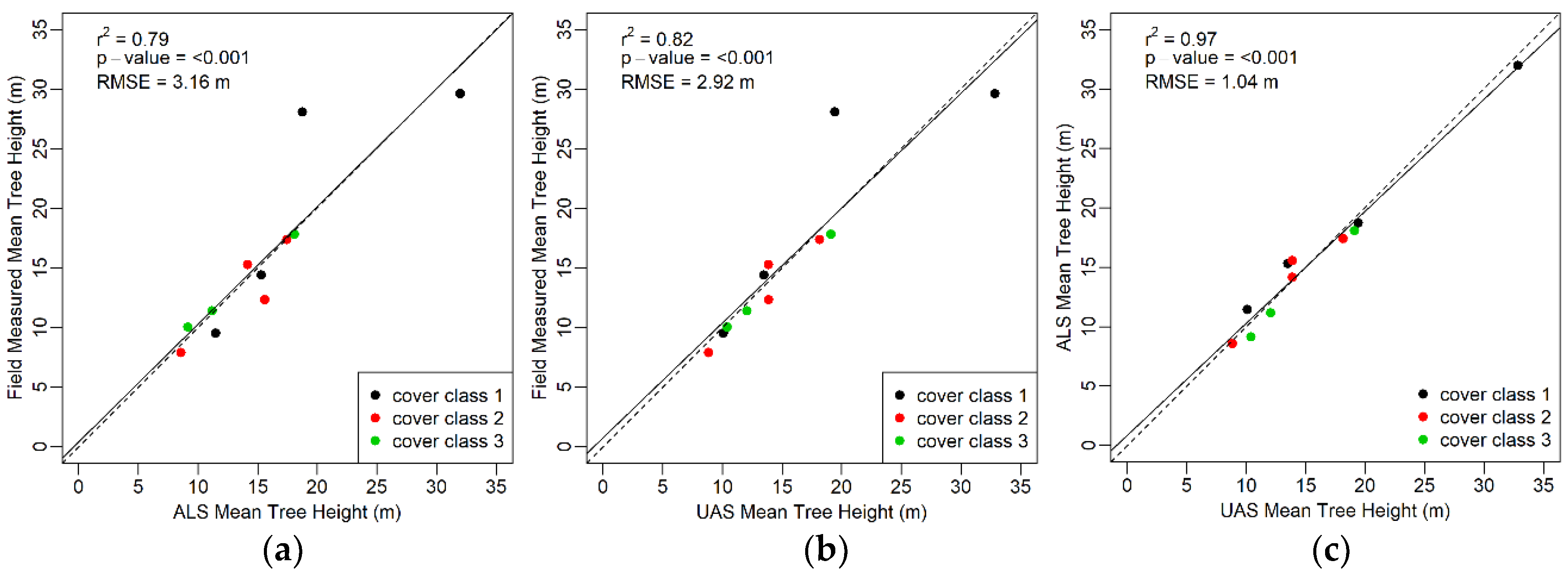
Figure 3 shows the UAS and ALS point clouds for one plot in each canopy cover class. The remote sensing methods demonstrate excellent registration to each other. The magnitude of relative registration discrepancies between each ALS and corresponding UAS point cloud was performed via the ICP algorithm [43] embedded in the CloudCompare software package [44]. The mean three-dimensional discrepancy across all plots was 0.193 m with standard deviation of 0.060 m. It is smaller than the nominal laser pulse footprint diameter in the study area. The directional (X, Y, Z), and overall (3D) residual GCP error mean (and standard deviation) across all 11 plots calculated by the Agisoft Photoscan software was 0.246 (0.089), 0.262 (0.062), 0.052 (0.036), and 0.371 m (0.084 m), respectively.

The point clouds from photogrammetry were substantially denser than those from ALS. The mean per square meter point density on the plots was, respectively, 1462.9 (SD = 624.8) and 5.0 (SD = 1.4) for photogrammetry and ALS. The increased point density in the photogrammetric point clouds can result in wider and more continuous canopy representation and improved measurement of canopy tops [45,46].

The optimal CHM resolution (

Table 3. Plot composite summaries by canopy cover class (CC) and inventory method. CC1 describes plots that had 10–40% canopy cover; CC2 40–70% canopy cover; and CC3 70–100% canopy cover.

	Field			ALS			UAS
	CC1	CC2	CC3	CC1	CC2	CC3	CC1	CC2	CC3
CHM cell resolution	--	--	--	3.0	0.3	0.2	2.5	0.4	0.3
Tree counts	36.0	62.0	159.0	30.0	47.0	125.0	30.0	63.0	139.0
Median tree height (m)	16.6	11.7	11.3	14.5	13.5	10.4	12.4	12.0	11.3
Mean tree height (m)	18.6	14.0	12.5	17.8	15.3	11.5	15.8	14.4	12.4
SD tree height	10.3	7.9	4.3	9.2	8.3	4.1	8.9	7.6	4.1
Min tree height (m)	5.5	6.4	5.5	8.5	7.7	7.7	8.0	7.9	7.9
Max tree height (m)	35.7	43.9	28.4	36.3	42.0	25.6	36.8	41.9	27.8

) was found to get finer with increasingly dense canopies using both ALS- and UAS-based methods.

3.2. Tree Metrics

The distributions of individual tree heights observed or predicted on the plots are similar across the field measurements and remote sensing methods (Table 3; Figure 4). Using field measurements as reference, median and mean tree heights were underestimated by remote sensing on cover class 1 plots, however, the UAS-derived estimates align remarkably well on plots of denser canopy cover. The differences in mean tree height between methods by canopy class are nonsignificant as determined by two-way ANOVA (F(4,682) = 1.55, p = 0.19). Minimum tree heights are noticeably smaller in the field measurements, while the minimum heights extracted from the point clouds correspond to the imposed 7.7-m height threshold. Maximum heights are larger in the ALS- and UAS-derived estimates for cover class 1 but smaller for classes 2 and 3.

Summaries of the agreement of tree counts and tree heights between the remote sensing methods and the ground-survey data are presented in

Table 4. Differences in optimized cell resolutions and plot composite summaries of remote sensing methods compared to in situ measurements. CC1 describes plots that had 10–40% canopy cover; CC2 plots had 40–70% canopy cover; and CC3 plots had 70–100% canopy cover.

	ALS vs. Field Measured			UAS vs. Field Measured
	CC1	CC2	CC3	CC1	CC2	CC3
CHM cell resolution	2.50	0.40	0.30	3.00	0.30	0.20
Mean difference in tree counts (n)	−1.50	−3.75	−11.33	−1.50	0.25	−6.67
Mean difference in min tree height (m)	4.09	0.62	1.77	4.23	0.99	1.72
Mean difference in mean tree height (m)	−1.04	0.70	−0.30	−1.47	0.44	0.73
Mean difference in max tree height (m)	0.22	−0.76	−1.71	0.17	-0.68	−1.01

. Except for estimates derived from the UAS method on canopy cover class 2 plots, the predicted number of trees from remote sensing underestimates the number found in the field on average. Performance of ITD is worst in cover class 3. Tree counts from photogrammetry-based ITD appear to be marginally superior to those derived from the LiDAR data. Overall, the height estimates obtained with remote sensing are comparable to and at the low end of the 1–5-m error range typically observed in conventional ground height measurements performed in the field [47].

The relationship among plot-specific tree number and mean height estimates is shown in Figure 5 and Figure 6, respectively. The remote-sensing-derived estimates of tree counts approximate the number of trees observed in the field well (ALS r² = 0.93, UAS r² = 0.84) and demonstrate excellent consensus with each other (r² = 0.96). Tree counts in cover class 3 are the least precise when compared to field measurements. The various methods are also congruent when measuring mean tree height. Strong correlation is observed between field-measured data and ALS-derived estimates (r² = 0.79) as well as UAS-collected data (r² = 0.82). ALS mean height exhibited an RMSE of 3.16 m, while the prediction of photogrammetric mean height gave an RMSE of 2.92 m. Again, the remote sensing methods agree with each other (r² = 0.97, RMSE = 1.04 m). Disregarding canopy cover designation, the ALS-derived tree count is more highly correlated to the number of trees measured in the field than the photogrammetric estimates. In estimating tree number mean height, the photogrammetric estimates appear to perform slightly better than those derived from ALS.

3.3. Growth Observations

Tree height metrics across canopy classes displayed in Table 4 do not conform to a unified pattern. Some of the UAS-derived height estimates appear to demonstrate growth, such as when they are greater than those observed in both the field and ALS-derived representations. Even when the photogrammetric height estimates are smaller than those measured in the field, some are closer to parity than the ALS-based measurements, thus indicating a positive change in height. Moreover, as evident in Figure 6a,b, mean plot tree height assessed from the UAS workflow is more closely aligned to the 1:1 line and was recorded with less error than mean plot height calculated from the ALS point clouds. However, we did not observe any unequivocable results indicating growth in the intervening two years between data acquisitions.

4. Discussion

4.1. Reconstructions

The suggested optimal CHM resolution was finer with progressively dense canopies. Optimal CHM resolution, in terms of ITD, correlates better with crown size than canopy cover. Where canopy cover is high, resource competition among trees prioritizes height growth for most species, thus accounting for a reduced crown diameter and CHM kernel size. While CHM parameters have been suggested for LiDAR point clouds [40,41], more research is needed to determine the effect of varying CHM resolutions on photogrammetric point clouds.

The two remote sensing methods used in this study are fundamentally different and do not observe forest structure the same way. ALS uses active systems and emits pulses of light backscattered by targets. Pulse photons not intercepted by foliage or branches near the top of a tree crown continue to penetrate the vegetation profile. A portion of them, often small but usually still identifiable even in high canopy cover forest stands, is ultimately backscattered by the ground and provides terrain reference. ALS point clouds are inherently three-dimensional products directly associated with forest structure. Conversely, UAS photogrammetry relies on cameras, which are passive systems and depend on solar or ambient illumination. UAS-imagery-derived point clouds contain 3D information obtained by inference but not directly. Their construction can suffer from some characteristics common to forest scenes, including weak geometry, homogeneous texture, object similarity, overlapping features, occlusion, and deep shadows, especially in small crown and stand openings. All these conditions degrade the performance of featured-based matching algorithms [48]. Flying at solar noon or on cloudy but bright days in low wind and with high image overlap helps mitigate these difficulties [49]. A comprehensive and detailed discussion regarding photogrammetry-based workflows is available in [50].

With UAS point clouds typically representing only the peripheral and usually upper components of dominant and codominant tree crowns, inventory parameters pertaining to the entire vertical profile of individual trees or forest stands, including tree height, can be challenging to access reliably because ground references are missing. It is thus not surprising that UAS-based estimates of tree height in close stands can be poor compared to those obtained by ALS [3]. DSMs obtained from digital imagery, however, are not subject to the many of the aforementioned limitations and can offer more reliable measurements of parameters manifested primarily in two dimensions, including ITD.

In this study, we attempted to circumvent this issue by using available, ALS-derived DTMs. We also included oblique imagery instead of the typical nadir-oriented imagery. Our alternative flight configuration increases flight and data-processing times but not substantially. Oblique imagery improves the viewing angle towards crown components that have primarily vertical orientation, such as the leading stems of conifers and, consequently, the probability that those components will be represented in the point cloud. It also improves the representation of components in the lower periphery of tree crowns. With more detailed representation of tree tops and crown edges, ITD performance is expected to improve.

Despite the presence of shadows during imagery capture on some plots, there were no discernible differences in performance in this study and the ultimate effect of shadows may be indiscriminate. Dandois and Ellis [20] posit that shadows in digital imagery hinder canopy penetration, but diffuse lighting reduces contrast and, therefore, feature matching. In conducive canopy cover and density conditions, tree height can be assessed from the cast shadows recorded in RGB photographs [49,51]. Advancement in photogrammetry and feature matching will continue to address known limitations, and indeed, meaningful alignment and depth maps are already available from inferior digital imagery, as demonstrated herein and by others [52,53].

4.2. Tree Metrics

Estimates of tree density were fairly well approximated in the UAS- and ALS-based inventory methods. As expected, tree counts in cover class 3 were the least precise when compared to field measurements. However, this was observed to be a disadvantage of both UAS and ALS remote sensing in this study. The lower tree omission rate of the photogrammetry-based ITD was not expected due to LiDAR’s improved ability to penetrate canopy, but it could have been influenced by the temporal discrepancy between the UAS flights and the field visits. In the two growing seasons between field inventory and UAS flight campaigns, certain trees could have cleared the height threshold we applied; or, it is an indication that the applied height threshold is slightly too aggressive, especially on plots with low canopy cover, where growth is likely concentrated in width rather than height. Our results indicate that the multiscopic sightings of canopy structure enabled by oblique imagery contributed to reducing errors embedded in the photogrammetric surface models, but further study should be done on height profiles obtained from similar UAS workflows.

Mean and median heights were most noticeably underestimated on cover class 1 plots, which suggests misidentification or omission of trees on these plots. Although covering less than 40% of a plot’s footprint in total, cover class 1 plots exhibit clusters of trees with overlapping crowns that would make differentiation during photogrammetry and ITD difficult. A regular pattern with gaps in the canopy would likely improve height estimation. The UAS-derived estimates followed the distribution of heights observed in field measurements more closely than the ALS-derived heights, although no definitive evidence was given for either method. There is currently no consensus on which remote sensing method is superior in regards to error, with respective research finding both photogrammetry and ALS performance better in some cases, but the magnitude of error is similar to that observed in other studies [11,54,55] and the correlation between photogrammetry and ALS tree heights is strong. It is possible to draw similar conclusions from either remote sensing method, suggesting that the more economical and approachable UAS methods can supplant ALS in iterative inventories.

4.3. Growth Observations

We expected less agreement between the ground-surveyed and photogrammetric-interpolated heights compared to the LiDAR equivalents due to the two-year time offset in measurement, but their atemporal agreement may have to do with measurement error in field heights. An improved ability to capture tree tops may be another explanation for those heights that are greater using the UAS method. Both field and ALS-based methods can fail to measure the tops of trees. Laser range finders and clinometers used by field crews can sometimes miscalculate tree heights when the tops of trees are obscured [47], in the presence of substantial tree lean [56], or where LiDAR pulses fail to systematically illuminate the leading tree stems [46], thereby inducting bias in tree and canopy height metrics.

After two years, higher mean and maximum tree heights were only systematically observed in the densest plots. Plots in the highest canopy cover had higher tree density and shorter height, typical of younger trees and of growth rates that are detectable and quantifiable at the short time scale between data acquisitions. Stands of mixed lodgepole and ponderosa pines experience mean annual height growth of 0.37 m when young [57], with growth plateauing after maturity is reached—anywhere from 70 to 300 years and heights from 20 to 60 m for ponderosa pines and around 100 years and between 21 and 24 m for lodgepole pines in Oregon [58,59]. With maximum observed tree height on any cover class 3 plot under 30 m, accelerated growth regimes would be the norm rather than the exception. Moreover, dense plots, where competition is increased, often promote height over canopy growth.

Owing to the short temporal discrepancy between field/ALS data collection and UAS flights and the limited number of plots used in this study, it is challenging to determine with confidence whether the differences in heights observed are due to growth, data acquisition type, propagation of measurement error, or technical and procedural limitations. Dempewolf et al. [31] suggest that high-precision differential GPS is needed for growth studies of individual trees to improve camera position accuracy and distortion calibration. Moreover, [19] established strong agreement between LiDAR and photogrammetry estimates of top of canopy height in tropical forests despite a similar two-year difference in data collection between the methods, suggesting growth may not be elucidated at this temporal scale when relying on consumer-grade GPS. Intraseasonal to decadal stand growth studies are available using a UAS and photogrammetry [20,30,31,60], but more attention is needed to provide low-cost solutions to improve reference datasets, such as ground surveys and geopositioning, to increase growth resolution.

4.4. Future Applications

This study would benefit from enumeration of all trees regardless of DBH. Avoidable error is introduced currently by approximating which “small” trees to remove in the point clouds to make data sources comparable. Although unequal stratified measurement is common of and necessary for large-area ground surveying [2], seedlings and saplings do not have a substantial impact on volume, biomass, and other ecological estimates. More exact measurement of tree heights during field collection would help to explain the observed differences between methods. However, the use of more accurate and precise measurement tools, such as survey stations, are logistically and economically infeasible for large-scale inventory operations such as those conducted by FIA. Although the use of a high-precision differential GPS would have improved the accuracy of tree height estimates and our ability to better quantify growth, meaningful height summaries were derived from a workflow leveraging consumer-grade, inexpensive GPS that was directly comparable to the performance of ground surveying and ALS. This method relies on quotidian GPS technology that requires no additional skill or knowledge in placing base stations, waypoint averaging, or performing direct georeferencing via a Helmert transformation [53]. A finer analysis of ITD could also illuminate model parameters and explanation of results. With the data collected through this study, further work could quantify tree locations and omission and commission rates, as demonstrated in other research [29,54].

As it is, the ultimate performance of the photogrammetric method was in part determined by existing data, namely, tree characterization from ground surveys and the DTM derived from ALS. However, this study was meant to demonstrate vertical development of an established forestry program, providing the capacity to advance preceding forest inventories with innovative remote sensing and computer vision technology. The motivation was to parametrize flight plans, canopy height models, and individual tree identification so that further data collection on FIA plots in Oregon and elsewhere can be conducted frequently and rapidly. Not only will regular UAS flights and point cloud processing improve studies of forest growth, but the workflow can also be implemented in reactive studies of forest disturbance. UAS data collection has been applied in real time for forest wildfire management [18] and could be an important tool in postfire monitoring.

Conversely, it is costly to conduct ground surveys and ALS frequently, but after initial collection, their products can continue to be referenced over time. The number of trees on a plot can be expected to remain relatively stable year to year and any necessary adjustments can be made quickly while on-site. The topographic terrain underlying the forest floor, as modeled from a LiDAR DTM, does not undergo substantial change annually and can be leveraged for multiple years in tandem with renewed DSMs derived from UASs to update forest inventories [19,22]. Moreover, baseline LiDAR products are becoming more ubiquitous and accessible for the general public. For instance, nearly 40% of Oregon forestland is currently covered by publicly available DTMs with plans to expand coverage [61], supporting this method as a viable option for repeat, low-cost surveying in many areas. The ongoing USGS 3DEP program aims at providing fine-resolution DTMs for the entire country [62].

Thus, this workflow provides nonforestry professionals and individuals with access to baseline forest resource assessment. The inclusion of these users is supported by advancements in autonomous flight and user interfaces for processing. Additionally, consumer RGB cameras are not only inexpensive but allow for more intuitive visual feature interpretation and display as well as the identification of species and assessment of health and stand maturity that is not readily available from ALS data. The data may even be leveraged for retrospective research questions as a high-density UAS point cloud provides digital preservation of the plot canopy in time with low-level, minimally processed data. If a particular measure becomes of interest in the future, it can likely be extracted from the point cloud, but it can never be retroactively recorded in field measurement. Photogrammetry has been gradually refined from its initial analog form after digital input became possible. In recent years, there has been exponential advancement in photogrammetric software development. Yet, there are many processing parameters the influence of which has not been clearly articulated. When the configuration of these parameters is optimized, we expect the conversion from digital images to complex representations of objects to become a rote process. In short, our method capitalizes on the ease, efficiency, affordability, and potential of commercial small-UAS hardware and computer vision software to open the field of forest management and evaluation to individuals and resource-constrained organizations.

5. Conclusions

In this study, we highlighted the performance of a UAS and photogrammetry to assess tree density and height on 11 plots in central Oregon. We compared and contrasted results gained from the photogrammetric workflow to those obtained via field measurements and ALS. The alternative method we presented here aids institutional and longitudinal forest inventories using affordable, commercial UAS hardware and photogrammetry software and it is sufficient to establish a comprehensive representation of forest plots. There was not enough evidence to describe the differences between the UAS-derived measurements and other methods as growth over the two-year measurement interval, but there is potential to quantify growth with similar methodologies as others have shown. Multitemporal monitoring should still be of interest on these plots in order to continue observation of patterns in photogrammetry performance and stand characteristics.

This was also a demonstration of incorporation of a new data source into an existing forestry program, considering all its inherent and known limitations. As this method was meant to broaden ongoing forest monitoring, it is not concerned by its initial reliance on historical data. In fact, it has shown that meaningful stand characteristics can be achieved even when data cannot be collected contemporaneously due to resources, program timelines, and retrospective research. This further increases its relevancy to private, nonindustrial forestland owners who will have some flexibility to obtain reasonable results despite their work not being exactly aligned with external data. This study supports the expansion of the legacy of public forest monitoring and heralds it into the next era of technological application and public crowdsourcing of forest data.

References

1. UN Food and Agriculture Organization. FRA 2015 Pprocess Document; United Nations: New York, NY, USA, 2016. [Google Scholar]
2. USDA Forest Service. Forest Inventory and Analysis National Core Field Guide, Volume 1: Field Data Collection Procedures for Phase 2 Plots; version 7.2; USDA Forest Service: Washington, DC, USA, 2017.
3. Mlambo, R.; Woodhouse, I.H.; Gerard, F.; Anderson, K. Structure from motion (SfM) photogrammetry with drone data: A low cost method for monitoring greenhouse gas emissions from forests in developing countries. Forests 2017, 8. [Google Scholar] [CrossRef]
4. United Nations. UN-REDD Programme Strategy 20112015; United Nations: New York, NY, USA, 2011. [Google Scholar]
5. Goodbody, T.R.H.; Coops, N.C.; Marshall, P.L.; Tompalski, P.; Crawford, P. Unmanned aerial systems for precision forest inventory purposes: A review and case study. For. Chron. 2017, 93, 71–81. [Google Scholar] [CrossRef] [Green Version]
6. Næsset, E. Airborne laser scanning as a method in operational forest inventory: Status of accuracy assessments accomplished in Scandinavia. Scand. J. For. Res. 2007, 22, 433–442. [Google Scholar] [CrossRef]
7. Anderson, K.; Gaston, K.J. Lightweight unmanned aerial vehicles will revolutionize spatial ecology. Front. Ecol. Environ. 2013, 11, 138–146. [Google Scholar] [CrossRef] [Green Version]
8. Hummel, S.; Hudak, A.T.; Uebler, E.H.; Falkowski, M.J.; Megown, K.A. A comparison of accuracy and cost of LiDAR versus stand exam data for landscape management on the Malheur National Forest. J. For. 2011, 267–273. [Google Scholar]
9. Snavely, N.; Seitz, S.M.; Szeliski, R. Modeling the World from Internet Photo Collections. Int. J. Comput. Vis. 2008, 80, 189–210. [Google Scholar] [CrossRef]
10. Probst, A.; Gatziolis, D.; Liénard, J.F.; Strigul, N. Intercomparison of photogrammetry software for three-dimensional vegetation modelling. R. Soc. Open Sci. 2018, 5. [Google Scholar] [CrossRef] [PubMed]
11. Wallace, L.; Lucieer, A.; Malenovský, Z.; Turner, D.; Vopěnka, P. Assessment of forest structure using two UAV techniques: A comparison of airborne laser scanning and structure from motion (SfM) point clouds. Forests 2016, 7. [Google Scholar] [CrossRef]
12. Wallace, L.; Lucieer, A.; Watson, C.S. Evaluating tree detection and segmentation routines on very high resolution UAV LiDAR data. IEEE Trans. Geosci. Remote Sens. 2014, 52, 7619–7628. [Google Scholar] [CrossRef]
13. Colomina, I.; Molina, P. Unmanned aerial systems for photogrammetry and remote sensing: A review. ISPRS J. Photogramm. Remote Sens. 2014, 92, 79–97. [Google Scholar] [CrossRef]
14. Oborne, M. Mission Planner v.1.3.45. Available online: www.ardupilot.org/planner (accessed on 6 August 2018).
15. DroidPlanner Labs. Tower v.1.4.0.1 Beta 1. Available online: www.play.google.com (accessed on 6 August 2018).
16. Agisoft, L.L.C. Photoscan Professional Edition v.1.4.2. Available online: www.agisoft.com (accessed on 6 August 2018).
17. McGaughey, R.J. FUSION/LIDAR Data Viewer and LIDAR Toolkit v.3.6. Available online: www.forsys.cfr.washington.edu/fusion/fusion_overview.html (accessed on 6 August 2018).
18. Tang, L.; Shao, G. Drone remote sensing for forestry research and practices. J. For. Res. 2015, 26, 791–797. [Google Scholar] [CrossRef]
19. Messinger, M.; Asner, G.P.; Silman, M. Rapid assessments of Amazon forest structure and biomass using small unmanned aerial systems. Remote Sens. 2016, 8. [Google Scholar] [CrossRef]
20. Dandois, J.P.; Ellis, E.C. High spatial resolution three-dimensional mapping of vegetation spectral dynamics using computer vision. Remote Sens. Environ. 2013, 136, 259–276. [Google Scholar] [CrossRef]
21. Gatziolis, D.; Liénard, J.F.; Vogs, A.; Strigul, N.S. 3D tree dimensionality assessment using photogrammetry and small unmanned aerial vehicles. PLoS ONE 2015, 10. [Google Scholar] [CrossRef] [PubMed]
22. Lisein, J.; Pierrot-Deseilligny, M.; Bonnet, S.; Lejeune, P. A photogrammetric workflow for the creation of a forest canopy height model from small unmanned aerial system imagery. Forests 2013, 4, 922–944. [Google Scholar] [CrossRef]
23. Puliti, S.; Ørka, H.O.; Gobakken, T.; Næsset, E. Inventory of small forest areas using an unmanned aerial system. Remote Sens. 2015, 7, 9632–9654. [Google Scholar] [CrossRef] [Green Version]
24. Gougeon, F.A. A Crown-Following Approach to the Automatic Delineation of Individual Tree Crowns in High Spatial Resolution Aerial Images. Can. J. Remote Sens. 1995, 21, 274–284. [Google Scholar] [CrossRef]
25. Wulder, M.; Niemann, K.O.; Goodenough, D.G. Local Maximum Filtering for the Extraction of Tree Locations and Basal Area from High Spatial Resolution Imagery. Remote Sens. Environ. 2000, 73, 103–114. [Google Scholar] [CrossRef]
26. Alonzo, M.; Andersen, H.-E.; Morton, D.C.; Cook, B.D. Quantifying Boreal Forest Structure and Composition Using UAV Structure from Motion. Forests 2018, 9. [Google Scholar] [CrossRef]
27. Dalponte, M.; Frizzera, L.; Ørka, H.O.; Gobakken, T.; Næsset, E.; Gianelle, D. Predicting stem diameters and aboveground biomass of individual trees using remote sensing data. Ecol. Indic. 2018, 85, 367–376. [Google Scholar] [CrossRef]
28. Jeronimo, S.M.A.; Kane, V.R.; Churchill, D.J.; McGaughey, R.J.; Franklin, J.F. Applying LiDAR Individual Tree Detection to Management of Structurally Diverse Forest Landscapes. J. For. 2018, 116, 336–346. [Google Scholar] [CrossRef]
29. Mohan, M.; Silva, C.A.; Klauberg, C.; Jat, P.; Catts, G.; Cardil, A.; Hudak, A.T.; Dia, M. Individual tree detection from unmanned aerial vehicle (UAV) derived canopy height model in an open canopy mixed conifer forest. Forests 2017, 8. [Google Scholar] [CrossRef]
30. Malambo, L.; Popescu, S.C.; Murray, S.C.; Putman, E.; Pugh, N.A.; Horne, D.W.; Richardson, G.; Sheridan, R.; Rooney, W.L.; Avant, R.; et al. Multitemporal field-based plant height estimation using 3D point clouds generated from small unmanned aerial systems high-resolution imagery. Int. J. Appl. Earth Obs. Geoinf. 2018, 64, 31–42. [Google Scholar] [CrossRef]
31. Dempewolf, J.; Nagol, J.; Hein, S.; Thiel, C.; Zimmermann, R. Measurement of within-season tree height growth in a mixed forest stand using UAV imagery. Forests 2017, 8. [Google Scholar] [CrossRef]
32. Hawbaker, T.J.; Keuler, N.S.; Lesak, A.A.; Gobakken, T.; Contrucci, K.; Radeloff, V.C. Improved estimates of forest vegetation structure and biomass with a LiDAR-optimized sampling design. J. Geophys. Res. Biogeosci. 2009, 114. [Google Scholar] [CrossRef] [Green Version]
33. Woodall, C.; Williams, M.S. Sampling Protocol, Estimation, and Analysis Procedures for the down Woody Materials Indicator of the FIA Program; Gen. Tech. Rep. NC-256; USDA Forest Service, North Central Research Station: St. Paul, MN, USA, 2005. [Google Scholar]
34. McGaughey, R.J.; Ahmed, K.; Andersen, H.-E.; Reutebuch, S.E. Effect of Occupation Time on the Horizontal Accuracy of a Mapping-Grade GNSS Receiver under Dense Forest Canopy. Photogramm. Eng. Remote Sens. 2017, 83, 861–868. [Google Scholar] [CrossRef]
35. Fritz, A.; Kattenborn, T.; Koch, B. UAV-based photogrammetric point clouds: Tree stem mapping in open stands in comparison to terrestrial laser scanner point clouds. In Proceedings of the International Archives of the Photogrammetry, Remote Sensing and Spatial Information Sciences, Rostock, Germany, 21–24 May 2013; Volume XL-1/W2, pp. 141–146. [Google Scholar]
36. James, M.R.; Robson, S. Mitigating systematic error in topographic models derived from UAV and ground-based image networks. Earth Surf. Process. Landf. 2014, 39, 1413–1420. [Google Scholar] [CrossRef] [Green Version]
37. Whitehead, K.; Hugenholtz, C.H. Remote sensing of the environment with small unmanned aircraft systems (UASs), part 1: A review of progress and challenges. J. Unmanned Veh. Syst. 2014, 2, 69–85. [Google Scholar] [CrossRef]
38. Triggs, B.; McLauchlan, P.F.; Hartley, R.I.; Fitzgibbon, A.W. Bundle Adjustment a Modern Synthesis. In Vision Algorithms: Theory and Practice; Lecture Notes in Computer Science; Springer: Berlin/Heidelberg, Germany, 2000; Volume 1883, pp. 298–372. [Google Scholar]
39. McGaughey, R.J. FUSION/LDV: Software for LIDAR Data Analysis and Visualization; USDA Forest Service, Pacific Northwest Research Station: Portland, OR, USA, 2016; Available online: http://forsys.cfr.washington.edu/FUSION/fusion_overview.html (accessed on 22 September 2018).
40. Chen, Q.; Baldocchi, D.; Gong, P.; Kelly, M. Isolating individual trees in a savanna woodland using small footprint Lidar data. Photogramm. Eng. Remote Sens. 2006, 72, 923–932. [Google Scholar] [CrossRef]
41. Monnet, J.-M.; Mermin, E.; Chanussot, J.; Berger, F. Tree top detection using local maxima filtering: A parameter sensitivity analysis. In Proceedings of the 10th International Conference on LiDAR Applications for Assessing Forest Ecosystems Silvilaser, Freiburg, Germany, 14–17 September 2010. [Google Scholar]
42. Keyser, C. Westside Cascades (WC) Variant Overview Forest Vegetation Simulator; U.S. Department of Agriculture, Forest Service, Forest Management Service Center: Fort Collins, CO, USA, 2008.
43. Besl, P.; McKay, N.D. A Method for Registration of 3-D Shapes. IEEE Trans. Pattern Anal. Mach. Intell. 1992, 14, 239–256. [Google Scholar] [CrossRef]
44. CloudCompare, Version 2.6.1. GPL Software. 2015. Available online: http://www.cloudcompare.org (accessed on 22 September 2018).
45. St-Onge, B.A.; Achaichia, N. Measuring forest canopy height using a combination of lidar and aerial photography data. In Proceedings of the International Archives of Photogrammetry and Remote Sensing, Annapolis, MD, USA, 22–24 October 2001; Volume XXXIV-3/W4, pp. 131–137. [Google Scholar]
46. Baltsavias, E.; Gruen, A.; Eisenbeiss, H.; Zhang, L.; Waser, L.T. High-quality image matching and automated generation of 3D tree models. Int. J. Remote Sens. 2008, 29, 1243–1259. [Google Scholar] [CrossRef]
47. Larjavaara, M.; Muller-Landau, H.C. Measuring tree height: A quantitative comparison of two common field methods in a moist tropical forest. Methods Ecol. Evol. 2013, 4, 793–801. [Google Scholar] [CrossRef]
48. Chen, S.; Yuan, X.; Yuan, W.; Cai, Y. Poor textural image matching based on graph theory. In Proceedings of the International Archives of the Photogrammetry, Remote Sensing and Spatial Information Sciences, Prague, Czech Republic, 12–19 July 2016; Volume XLI-B3, pp. 741–747. [Google Scholar]
49. Seely, H.E. Computing tree heights from shadows in aerial photographs. For. Chron. 1929, 5, 24–27. [Google Scholar] [CrossRef]
50. Carrivick, J.L.; Smith, M.W.; Quincey, D.J. Structure from Motion in Geosciences. Wiley-Blackwell: Oxford, UK, 2016; p. 208. [Google Scholar]
51. Verma, N.K.; Lamb, D.W. The use of shadows in high spatial resolution, remotely sensed, imagery to estimate the height of individual Eucalyptus trees on undulating land. Rangel. J. 2015, 37, 467–476. [Google Scholar] [CrossRef]
52. Zarco-Tejada, P.J.; Diaz-Varela, R.; Angileri, V.; Loudjani, P. Tree height quantification using very high resolution imagery acquired from an unmanned aerial vehicle (UAV) and automatic 3D photo-reconstruction methods. Eur. J. Agron. 2014, 55, 89–99. [Google Scholar] [CrossRef] [Green Version]
53. Turner, D.; Lucieer, A.; Watson, C. An automated technique for generating georectified mosaics from ultra-high resolution unmanned aerial vehicle (UAV) imagery, based on structure from motion (SfM) point clouds. Remote Sens. 2012, 4, 1392–1410. [Google Scholar] [CrossRef]
54. Thiel, C.; Schmullius, C. Comparison of UAV photograph-based and airborne lidar-based point clouds over forest from a forestry application perspective. Int. J. Remote Sens. 2016, 38, 1–16. [Google Scholar] [CrossRef]
55. Sankey, T.; Donager, J.; McVay, J.; Sankey, J.B. UAV lidar and hyperspectral fusion for forest monitoring in the southwestern USA. Remote Sens. Environ. 2017, 195, 30–43. [Google Scholar] [CrossRef]
56. Gatziolis, D.; Fried, J.S.; Monleon, V.S. Challenges to estimating tree height via LiDAR in closed-canopy forest: A parable from western Oregon. For. Sci. 2010, 56, 139–155. [Google Scholar]
57. Seidel, K.W. A Ponderosa Pine-Lodgepole Pine Spacing Study in Central Oregon: Results after 20 Years; USDA Forest Service, Pacific Northwest Research Station: Portland, OR, USA, 1989. [Google Scholar]
58. Lowery, D.P. Ponderosa Pine; An American Wood; USDA Forest Service: Washington, DC, USA, 1984. [Google Scholar]
59. USDA NRCS Plant Materials Program. Plant Fact Sheet: Ponderosa Pine; USDA Natural Resources Conservation Science: Washington, DC, USA, 2002.
60. Zhang, J.; Hu, J.; Lian, J.; Fan, Z.; Ouyang, X.; Ye, W. Seeing the forest from drones: Testing the potential of lightweight drones as a tool for long-term forest monitoring. Biol. Conserv. 2016, 198, 60–69. [Google Scholar] [CrossRef]
61. DOGAMI (Oregon Department of Geology and Mineral Industries). Collecting LiDAR. Available online: http://www.oregongeology.org/lidar/collectinglidar.htm (accessed on 17 June 2018).
62. U.S. Geological Survey the National Map: 3D Elevation Program (3DEP). Available online: https://nationalmap.gov/3DEP/ (accessed on 5 August 2018).
Figure 1. Location of field plots sampled from Carbon Monitoring System (CMS) in Oregon.
Remotesensing 10 01562 g001
Figure 2. Flowchart of the methodology employed.
Remotesensing 10 01562 g002
Figure 3. Nadir views of 3D representations produced by unmanned aerial system (UAS)- and airborne laser scanning (ALS)-derived methods, respectively, from one plot in each canopy cover between (a,d) 10–40%; (b,e) 40–70%; and (c,f) 70–100%. The point clouds from imagery collected with the UAS are displayed in red, green, blue (RGB) while the point clouds obtained from ALS are colored according to aboveground height. The blue circle represents the boundary of the 16.2-m radius plot.
Remotesensing 10 01562 g003
Figure 4. Distribution of individual tree heights by inventory method in plots with canopy cover between (a) 10–40%; (b) 40–70%; (c) and 70–100%. The thick lines represent median heights while the bottom and top boundaries of the box show 25th and 75th, respectively, height percentiles. The ends of the whiskers are ±1.5 times the interquartile range and the circles are distributional outliers. Field corresponds to the in situ measurements, als to the estimates derived from ALS, and uas to estimates derived from UAS data collection and photogrammetry.
Remotesensing 10 01562 g004
Figure 5. (a) ALS-based and (b) UAS-photogrammetry-derived estimates of plot tree counts vs. field-measured counts or (c) vs. the opposing remote sensing method by canopy cover class. The solid line displays a linear regression fit and the dashed line the 1:1 line.
Remotesensing 10 01562 g005
Figure 6. (a) ALS-based and (b) UAS-photogrammetry-derived estimates of mean tree height vs. field-measured counts or (c) vs. the opposing remote sensing method by canopy cover class. The solid line displays a linear regression fit and the dashed line the 1:1 line.
Remotesensing 10 01562 g006