


Abstract
Thorough analysis of regional carbon emissions is essential, given their substantial contribution to overall carbon emissions, as it underpins the formulation of targeted low-carbon development strategies. This study investigates whether Hubei Province can achieve carbon peaking by 2030 and explores feasible emission reduction pathways. To address the limitations of existing regional carbon emission studies—particularly the direct use of decomposition factors in prediction models and the lack of logical separation between mechanism analysis and forecasting—a hybrid analytical-predictive framework is proposed. Specifically, the logarithmic mean Divisia index (LMDI) method is first employed to decompose historical carbon emissions and identify the driving forces, while the STIRPAT model combined with the Lasso regression is subsequently used to screen key influencing factors for emission prediction, thereby avoiding the direct use of decomposition factors in forecasting. Based on the selected factors, a genetic algorithm–optimized backpropagation neural network (GA-BP) is developed to predict carbon emissions in Hubei Province from 2024 to 2035. The predictive performance of the GA-BP model is validated using three statistical indicators (R2, MAPE, and RMSE) and compared with Extreme Learning Machine (ELM), Support Vector Regression (SVR), and conventional BP models. Furthermore, six development scenarios are designed in accordance with provincial policy objectives to assess the feasibility of carbon peaking. The results indicate the following: (1) Based on the results of the LMDI decomposition, Lasso–STIRPAT analysis, and model sensitivity analysis, per capita GDP is identified as the primary driving factor of carbon emissions in Hubei Province. (2) The GA-BP model demonstrates superior predictive accuracy compared with benchmark models and (3) carbon peaking by 2030 can only be achieved under Scenario 6, highlighting the necessity of coordinated structural and technological interventions. Based on these findings, targeted policy recommendations for carbon emission reduction are proposed.
1. Introduction
The extensive use of fossil fuels has led to anthropogenic climate change. This process is mainly driven by greenhouse gas emissions, especially CO2, and has become a major global environmental challenge. According to NOAA’s report [1], the atmospheric CO2 concentration reached 423.64 ppm in 2024. This sharp increase threatens the Earth’s ecosystems and undermines the sustainable development of social systems. Therefore, urgent and coordinated action from the international community is essential [2]. In response to this challenge, nearly 150 countries around the world have proposed carbon reduction targets—Zheng et al. [3]—including China, which has pledged to peak carbon dioxide emissions by 2030 and achieve carbon neutrality by 2060—Liu et al. [4]. As one of the world’s largest carbon emitters, China is proactively addressing the issue of deep carbon emission reductions while concurrently pursuing high-quality, environmentally sustainable economic and social development. In October 2021, the Chinese government issued the “Opinions on Doing a Good Job of Peak Carbon Achievement and Carbon Neutrality by Completely, Accurately, and Comprehensively Implementing the New Development Philosophy” [5]. This document summarizes the overall situation of peak carbon achievement and carbon neutrality and emphasizes that—based on the level of economic development, industrial structure, energy structure, resource endowment, and environmental conditions of each region—the objectives and pathways of peak carbon achievement should be determined scientifically and reasonably. However, existing studies on carbon emissions in China are mostly conducted at the national level, which may mask substantial regional heterogeneity in emission drivers and mitigation potential.
Against this backdrop, provincial administrative units, which serve as the primary implementers of regional carbon reduction policies, bear the main responsibility for emission mitigation. Consequently, investigating carbon emissions at the provincial level is of great importance [6,7].
Hubei Province, a key region in central China, features a heavy-industry-dominated industrial structure and an energy system heavily reliant on coal. Research on carbon emissions in Hubei Province is therefore of both theoretical and practical significance. This research is crucial for achieving national carbon peaking and carbon neutrality goals; formulating region-specific emission reduction strategies; optimizing the energy mix; promoting green and low-carbon transitions; and supporting the sustainable development of the regional economy. In this context, this paper aims to identify the key driving factors of carbon emissions in Hubei Province and to predict whether the province can achieve carbon peaking on schedule. Using data from the Hubei Statistical Yearbook covering the period from 2000 to 2023, the study provides a quantitative basis for formulating targeted strategies and policy recommendations to support the region’s low-carbon transition and sustainable development. The findings contribute to the development of targeted countermeasures and strategic recommendations for effectively achieving carbon neutrality amid rising regional carbon emissions. Furthermore, they provide a robust theoretical foundation for advancing sustainable development that prioritizes ecological integrity, low-carbon emissions, and high-quality growth.
The main contents of this paper are as follows: (1) This paper uses the LMDI decomposition method to identify key factors of carbon emissions in Hubei Province, and the research results show that energy intensity and per capita GDP are important influencing factors of carbon emissions. Based on the economic development and social conditions of Hubei Province as well as the key factors of the LMDI, this paper uses the STIRPAT model and the Lasso model to screen ten influencing factors. The influencing factors were determined to be seven factors: population (P), per capita GDP (G), energy structure (ES), energy intensity (EI), urbanization rate (U), industrial structure (IS), and the proportion of import and export trade volume (TIEV). (2) This paper establishes the ELM, SVR, BP, and GA-BP models, which are trained with the data from 2000 to 2017, verified with the data from 2018 to 2019, and tested from 2020 to 2023. By analyzing the training results of GA-BP, it is found that the learning and generalization ability of the GA-BP model itself is relatively high. Through comparative analysis, it is found that the GA-BP model performs the best among these models, and the GA effectively optimizes the internal initial weights and biases. (3) Based on Hubei Province’s “14th Five-Year Plan” and previous data, six scenarios were set up to discuss the impact of different development paths of energy intensity and energy structure on carbon emissions. The GA-BP model was adopted to predict the carbon emissions of Hubei Province from 2023 to 2035, and the peak values and peak times of carbon emissions under different scenarios were determined. Based on the above analysis and prediction, combined with the actual situation, this paper puts forward valuable suggestions for the carbon emission reduction path in Hubei Province. (4) Based on the calculation and simulation results, policy suggestions for carbon peaking and carbon emission reduction are put forward.
The rest of the paper is organized as follows: Section 2, “Literature Review”, summarizes the existing literature on carbon emission projections; Section 3, “Methods and Data”, offers a detailed account of the methodologies and data sources utilized in this study; Section 4, “Results and Discussion”, analyzes and discusses the results of the model; and Section 5, “Conclusions and Suggestions”, summarizes the full text and gives suggestions.
2. Literature Review
2.1. Review of Methods for Exploring Carbon Emission Factors
In the field of carbon emission research, scholars frequently utilize quantitative models to analyze the drivers of carbon emissions. Examples of such models include the STIRPAT expanded model [6,8], the logarithmic mean Divisia index (LMDI) [9,10], the Gross Domestic Input of Materials (GDIM) [11,12], and so on. For example, Yu and Du [13] employed the STIRPAT model to investigate the impacts of technological innovation on carbon emissions. The results revealed that indigenous innovation significantly promotes CO2 emissions, whereas imitative innovation demonstrates a suppressive effect on carbon output. Chen et al. [11] utilized GDIM to analyze the carbon emissions of global commercial buildings and found that the United States and China were the largest carbon emitters. Chen et al. [14] used the LMDI method to analyze China and found that economic output growth has a significant driving effect on carbon emissions, energy intensity reduction has a significant inhibiting effect on carbon emissions, and small fluctuations in energy structure have a small impact on carbon emissions. Lin and Li [15] used the LMDI model to explore carbon emission factors in Fujian Province, and the results showed that per capita GDP was the main positive driving factor, and Zhao et al. [16] used the LMDI to decompose carbon emissions of various countries and found that energy intensity and economic growth were the main driving factors for carbon emissions.
Based on the above literature, STIRPAT, based on regression analysis, allows for hypothesis testing and quantification of factor elasticity, but it is sensitive to multicollinearity, model specification, and data quality, which can lead to biased or inconsistent results across regions. The LMDI, in contrast, provides exact decomposition without residuals and is widely appreciated for spatiotemporal and multi-scale analysis; however, it is fundamentally descriptive, cannot predict future emissions, and often ignores interactions among factors. GDIM can capture interaction effects and provide a more generalized decomposition framework, but its complexity, computational burden, and less intuitive interpretability limit its practical application, especially for policy analysis. Across these methods, inconsistencies can arise due to different factor definitions, aggregation levels, or methodological assumptions. For Hubei Province, with its coal-dependent energy structure and industrial-heavy economy, the LMDI method is particularly suitable for historical carbon emission decomposition due to its ability to provide exact, residual-free attribution of contributions from economic, energy, and structural factors. Compared with STIRPAT, which is sensitive to multicollinearity, and GDIM, which is computationally complex and less intuitive, the LMDI offers clear interpretability and robustness for multi-scale and spatiotemporal analysis. Based on this empirical foundation, this study adopts an improved LMDI method to systematically examine the driving factors of carbon emissions in Hubei Province.
2.2. Review of Carbon Emission Forecasting Methods
Carbon emission prediction methods mainly include a traditional mathematical statistics model and machine learning model. Although traditional models remain widely used due to their simplicity and strong interpretability, machine learning methods—particularly those based on deep learning—have rapidly emerged in recent years, driven by their powerful nonlinear representation capabilities. It is worth noting that, with the advancement of artificial intelligence technologies, researchers are increasingly adopting neural network architectures integrated with optimization algorithms. These models significantly enhance the generalization ability and prediction accuracy through dynamic parameter adjustment mechanisms [17]. For example, Rao et al. [12] constructed the GA-BP model to predict carbon emission, and the results showed that the carbon emission constraint in the Pearl River Delta region could not be achieved until 2035; Ren and Long [18] constructed nine scenarios and used the CSO-FLN model to predict whether the carbon emission of Guangdong Province could meet the target of peaking carbon neutrality on time. The results showed that only one scenario could meet the target on time. Shi et al. [19] used the STIRPAT model and Ridge regression to distinguish and rank the importance of China’s impact factors and constructed a GA-LSTM model for prediction. The results showed that energy consumption structure and industrial structure were the main influencing factors. China’s carbon emissions will peak at 1.163 billion tonnes around 2030. Furthermore, Li et al. [20] proposed a hybrid model that incorporates multimodal data, convolutional neural network inceptionv2 (CNN-inceptionv2), attention-mechanically optimized text convolutional neural networks (TextCNNs), and bidirectional long short-term memory (BiLSTM) to overcome carbon emission prediction relying on time-series data alone. And Li et al. [21] proposed a multi-factor combination prediction model named ICEEMDAN-LOBiLSTM-LOLSSVM to accurately predict carbon emissions.
Based on the above research, traditional statistical methods, such as linear regression and grey models, generally exhibit limited predictive accuracy and are incapable of capturing complex nonlinear relationships among carbon emission drivers. Conventional machine learning approaches, including BP neural networks, SVR, and ELM, improve nonlinear modeling capability but are prone to overfitting and often require extensive parameter tuning. To overcome these limitations, this study employs a genetic algorithm–optimized BP neural network (GA-BP), which enhances parameter selection, improves model stability, and increases predictive accuracy, making it particularly suitable for forecasting carbon emissions in Hubei Province under various development scenarios.
To summarize, the present study focused on Hubei Province. The LMDI method was used to develop a decomposition framework for the systematic analysis of carbon emission drivers. This analysis led to the development of a hybrid prediction model combining a genetic algorithm (GA) with a backpropagation (BP) neural network. This hybrid model was designed to optimize multiple parameters and avoid convergence to local minima. The model was then used to simulate carbon emission trends under various scenarios from 2024 to 2035. The results highlight potential pathways for low-carbon transformation in Hubei Province and provide policy recommendations.
3. Methods and Data
3.1. Study Area and Data
3.1.1. Overview of the Study Area
Hubei Province, located in central China, features rapid economic growth and high population density. In recent years, the province has experienced robust economic growth, with its GDP exceeding 6 trillion CNY in 2023. The province has made significant progress in post-pandemic recovery, with continued promotion of high-quality development initiatives. According to data from the Hubei Provincial Bureau of Statistics and the Seventh National Census [22], the permanent resident population was over 57 million, reflecting Hubei’s prominence as a national central city. Despite various challenges, the province’s economy has maintained steady growth. In 2023, the regional GDP growth rate reached 4.3%, ranking among the top provinces nationwide. Therefore, carbon emission prediction research in Hubei is highly representative in studies of socio-economic development and ecological governance.
3.1.2. The Calculation of Carbon Emissions
Carbon emission data: The carbon emission data in this article is mainly calculated based on the emission factor method provided in the “2006 IPCC Guidelines for National Greenhouse Gas Inventories” [23], as shown in Equation (1).
In the formula, Ci represents the carbon emissions generated by the i type of energy, NCVi represents the low calorific value of the i type of energy, CCi represents the carbon content per unit heat of the i type of energy, and COFi represents the carbon oxidation rate of the i type of energy, representing the ratio of carbon molecules in carbon dioxide. The carbon emission factors in this paper are calculated by the author according to the Guidelines for Compiling Provincial Greenhouse Gas Inventories (Trial) [24] and the Guidelines for Gas Accounting Methods and Reporting of the General Office of the National Development and Reform Commission (Trial) [25]. The correlation coefficients are shown in Table 1.
Table 1.
The carbon emission coefficient of energies.
3.2. LMDI Decomposition Model
Ang [26,27] compared various index decomposition analysis methods and concluded that log-average division (LMDI) is the preferred method for total decomposition. Therefore, this paper adopts the LMDI model to decompose carbon emissions into five influencing factors, including carbon emission intensity, energy structure, energy intensity, per capita GDP, and population size, as shown in the following equation:
where C represents carbon emissions, Ci represents carbon emissions generated by the i type of energy, Ei represents consumption of the i type of energy, E represents total energy consumption, GDP represents gross regional product, and P represents population size. F means carbon emission factor, ES means energy mix, EI means energy intensity, G means GDP per capita, and P means population size.
The contribution of each factor is measured according to Equation (3). The total energy consumption carbon emission in the base period is , and the total energy consumption carbon emission in the T period is . The LMDI additive decomposition method was used to calculate the contribution value of driving factors to carbon emissions in Hubei Province. The decomposition process is as follows:
The contribution value of each influence factor is obtained by LMDI method, as follows:
where is the total change in carbon emission from year 0 to year T. , , , , and represent the influence of carbon emission intensity, energy structure, energy intensity, per capita GDP, and population size on carbon emission, respectively.
3.3. Selection of Factors Influencing Carbon Emissions
Based on the previous work, combined with the decomposition factors of the LMDI and the unique regional characteristics of Hubei Province, a total of 10 carbon emission factors are selected in this paper. The STIRPAT [28] model and Lasso model [29] are used to clarify the degree of influence of each factor on carbon emissions, to screen out the significant variables that can reflect the trend of carbon emission changes, and to simplify the input data of the prediction model. The detailed calculation process and conclusions are shown in Appendix A.
After the screening of the Lasso model, a total of seven variables are selected as input variables of the prediction model in this paper, which are population (P), urbanization rate (U), per capita GDP (G), industrial structure (IS), energy structure (ES), energy intensity (EI), and total import and export trade as a proportion of GDP (TIEV). In this process, three variables—R&D investment, patents granted, and freight volume—were excluded because their coefficients shrank to zero under the Lasso penalty. The specific coefficients are shown in Table 2.
Table 2.
The result of the Lasso model.
Various economic and energy data source: the data of GDP, total energy consumption, and population size of Hubei Province are derived from the Hubei Provincial Statistical Yearbook and China Energy Statistical Yearbook, and some missing values are supplemented according to the data reported in the statistical yearbook of each city of Hubei Province.
3.4. GA-BP Neural Network
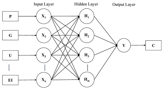
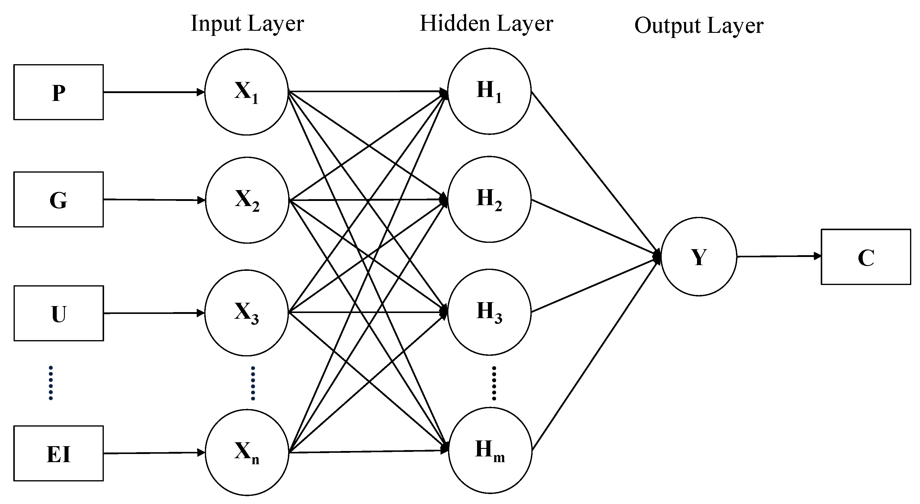
The BP neural network is a multi-layer feedforward neural network that learns through error backpropagation. Due to its relatively simple architecture and robust learning capabilities, it has become one of the most important and widely applied artificial neural network algorithms [30]. Specifically, a single-hidden-layer BP neural network can approximate any continuous function, making it particularly advantageous for handling nonlinear problems such as carbon emission prediction [2]. However, the initial weights and thresholds of the network significantly influence the accuracy of the final prediction results. To address this issue, the integration of genetic algorithms (GAs) can optimize the initial weights and thresholds of the BP neural network, thereby enhancing its prediction accuracy, generalization ability, and robustness [31]. In this study, we employ the GA-BP model for carbon emission prediction, and its performance is compared with the EVM, SVR, and BP models to evaluate predictive accuracy. And the GA-BP model consists of three layers: input layer, hidden layer, and output layer. Data are first received by the input layer, processed in the hidden layer, and then passed to the output layer where the results are calculated and output. The specific workflow is illustrated in Figure 1.
Figure 1.
The construction of the BP model.
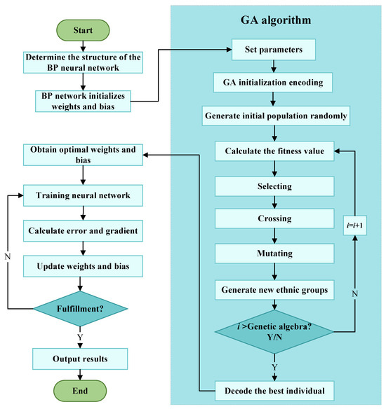
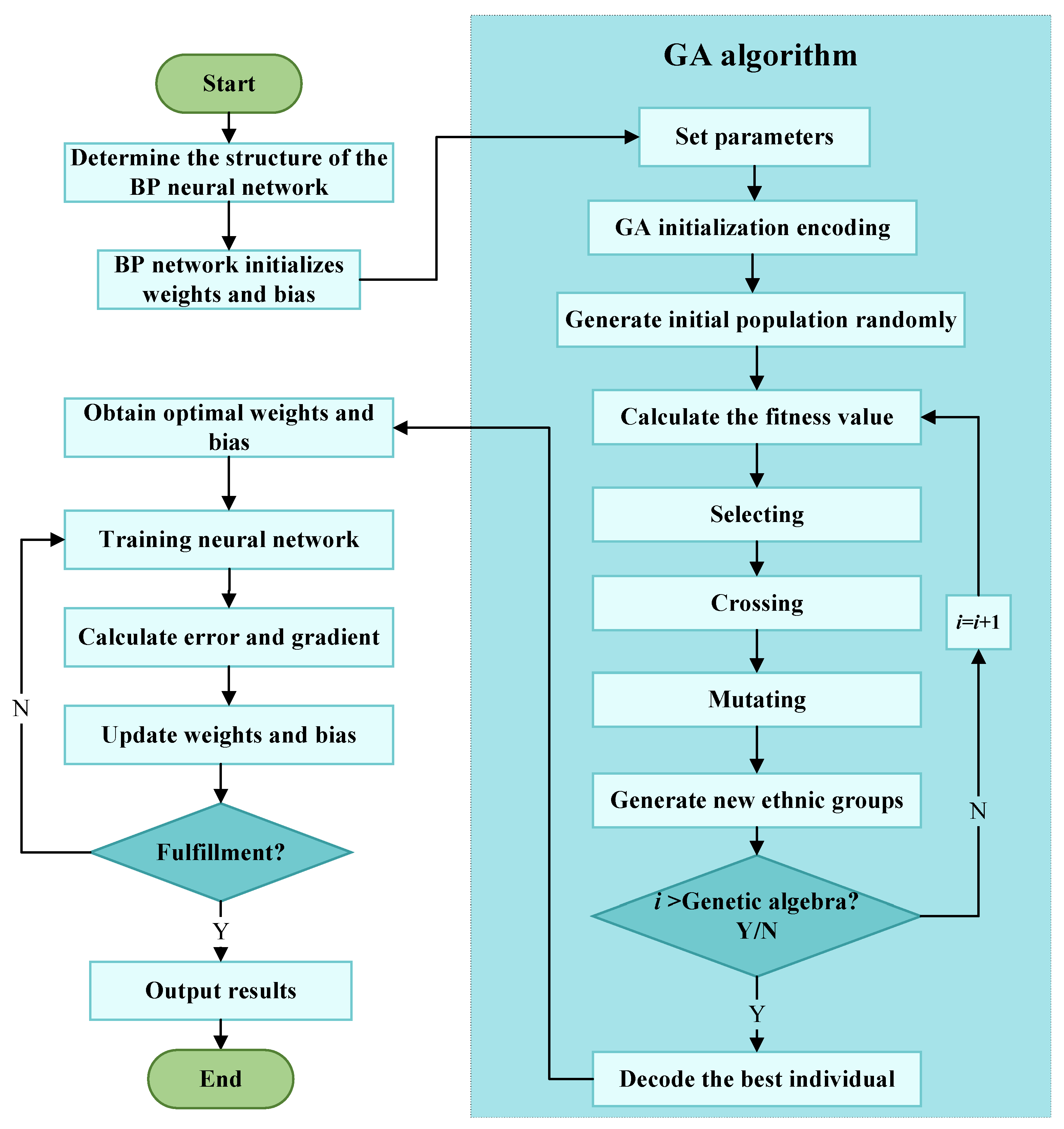
The GA-BP model incorporates the following steps, the specific process of which is illustrated in Figure 2.
Figure 2.
GA-BP model flow chart.
Step 1. Preprocessing. All the data are normalized, and the normalization scales the data to make it fall into a small specific interval [0,1], so as to eliminate the difference between data dimension and unit, and improve the convergence speed and stability of the model. The normalization formula is as follows:
Step 2. Calculating chromosome length and population initialization. The GA coding form in this paper adopts real-value coding, that is, the weight and bias of the neural network are directly used as genes on chromosomes, and the calculation formula for chromosome length is as follows:
Step 3. The fitness of the initial population is calculated. The fitness function is used to evaluate the performance of individuals in the neural network. In this study, the fitness function is related to the mean square error (MSE) of the model:
Step 4. Selecting. Selection operations refer to the selection of individuals from the current population to inherit into the next generation. In this study, the roulette method is adopted for selection, and individuals with high fitness are more likely to be selected, so as to realize the principle of “survival of the fittest” and promote the evolution of the population in a better direction. The probability of selection is calculated as follows:
Step 5. Crossing. Crossover operation means that in the case of meeting the crossover probability, another chromosome is selected, the crossover point is determined, and the gene of the chromosome is recombined at the crossover point so as to form a new individual.
Step 6. Mutating. Mutation operation will check each chromosome in the population. For chromosomes that meet the mutation probability, a gene coding position will be randomly selected and the gene coding position will be reversed to introduce a new gene combination, increase the genetic diversity of the population, and help the genetic algorithm to jump out of the local optimal solution and find a better global solution.
Step 7. Iteratively optimizing search. Depending on the number of iterations specified, the iterations perform steps 2–5, and each cycle is called population evolution. Then, the optimal individuals meeting the requirements are converted into the initial weights and thresholds of the BP neural network.
Step 8. Training. The optimal weight and bias obtained by the GA are used as the initial weight and bias input of the BP neural network. After the BP neural network is trained, the trained model is used to predict the data.
4. Results
4.1. Current Trends of Carbon Emissions
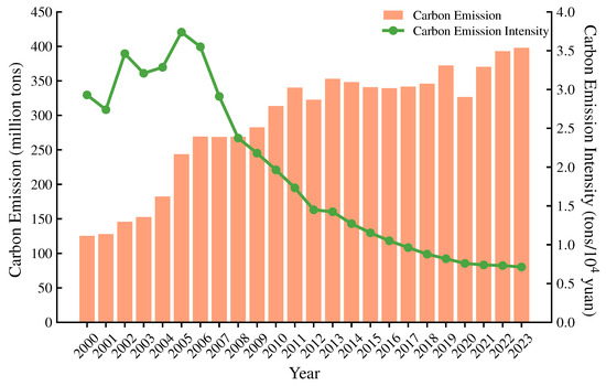
Based on (1) and the related data, the carbon emissions (C) and carbon emission intensity (CEI) of Hubei from 2000 to 2023 are obtained. CEI refers to the ratio of carbon emissions to GDP, and the specific calculation formula is as shown in Equation (13).
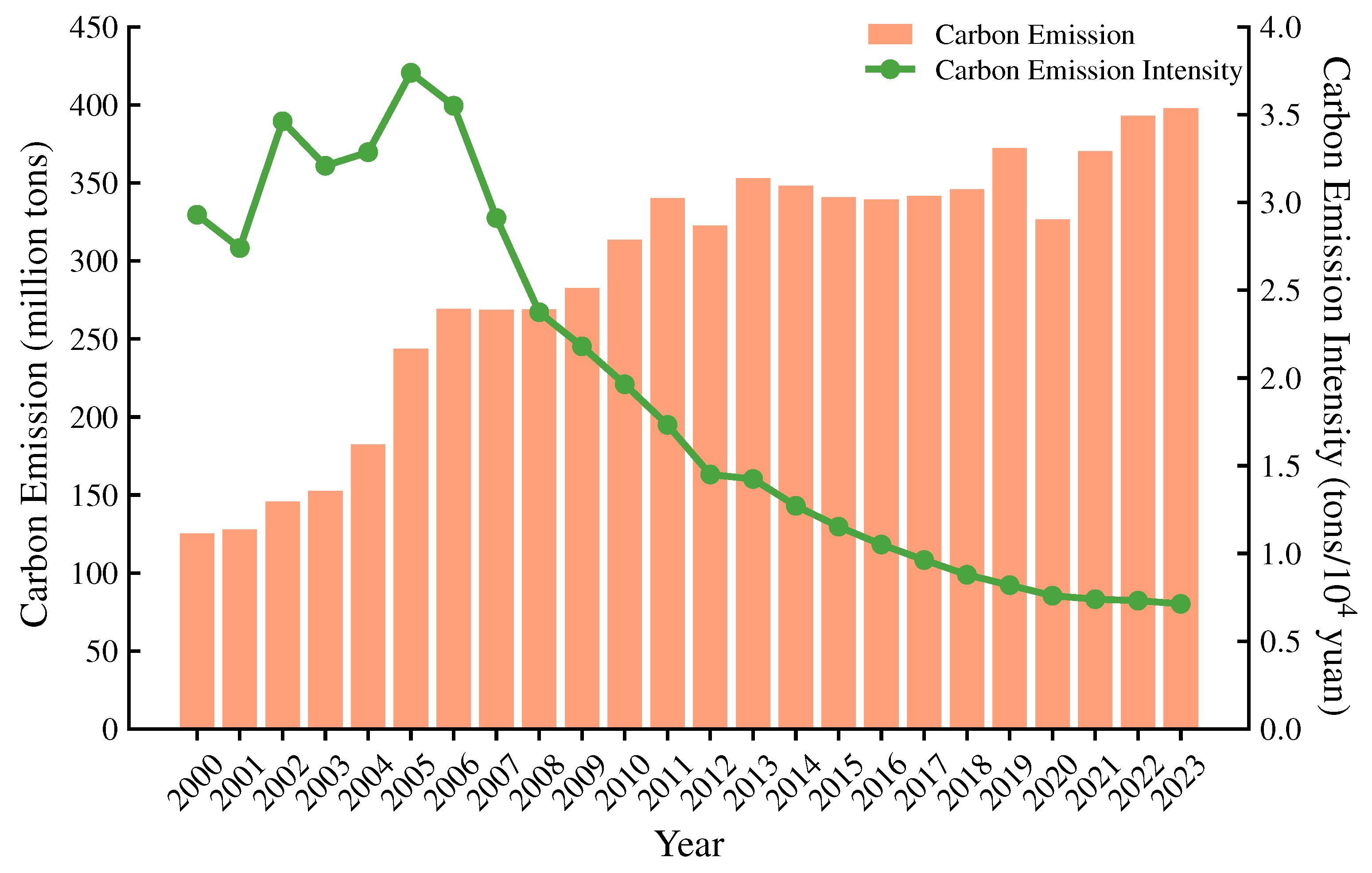
The results are shown in Figure 3. As shown in Figure 3, C in Hubei Province increased from 125.30 million tons in 2000 to 397.85 million tons in 2023, with an average annual growth rate of 5.529%, showing an upward trend; the intensity of carbon emissions decreased from 2.93 ton per CNY to 0.71 ton per CNY, showing a downward trend. Based on Figure 3, the C in Hubei demonstrated an overall upward trend, with a marked increase in carbon emissions from 2000 to 2013. The average annual growth rate was recorded as 8.7%. It may be hypothesized that during this period, Hubei was experiencing a process of industrialization, characterized by the dominance of heavy industries with high energy consumption and high emission, such as steel, the chemical industry, building materials, and electric power, which resulted in the rapid growth of carbon emissions.
Figure 3.
Trends of C and CEI in Hubei from 2000 to 2023.
From 2000 to 2005, carbon emissions in Hubei Province gradually increased, and carbon intensity exhibited a fluctuating upward trend. After 2005, however, carbon intensity began to decline continuously. This reversal can be attributed primarily to structural adjustments driven by national policy. During the 10th Five-Year Plan [32] period, the Chinese government explicitly emphasized energy conservation and emission reduction. In response, Hubei Province promoted industrial restructuring, gradually shifting from high-energy-consuming sectors toward higher value-added and less energy-intensive industries. This adjustment, together with the adoption of more efficient technologies and improved energy use, contributed to the observed decline in carbon intensity after 2005. Following 2013, the C demonstrated a decline in momentum, with a decrease observed in certain years. The average annual growth rate was recorded at 1.5%, a consequence of the intertwined influences of Hubei Province’s advanced economic development, the transformation of its energy structure, and the establishment of an ecological civilization. The substantial reduction in carbon emissions in 2020 may be associated with the emergence of the novel Coronavirus (SARS-CoV-2) pandemic [33].
4.2. Decomposition Results of Carbon Emission Factors
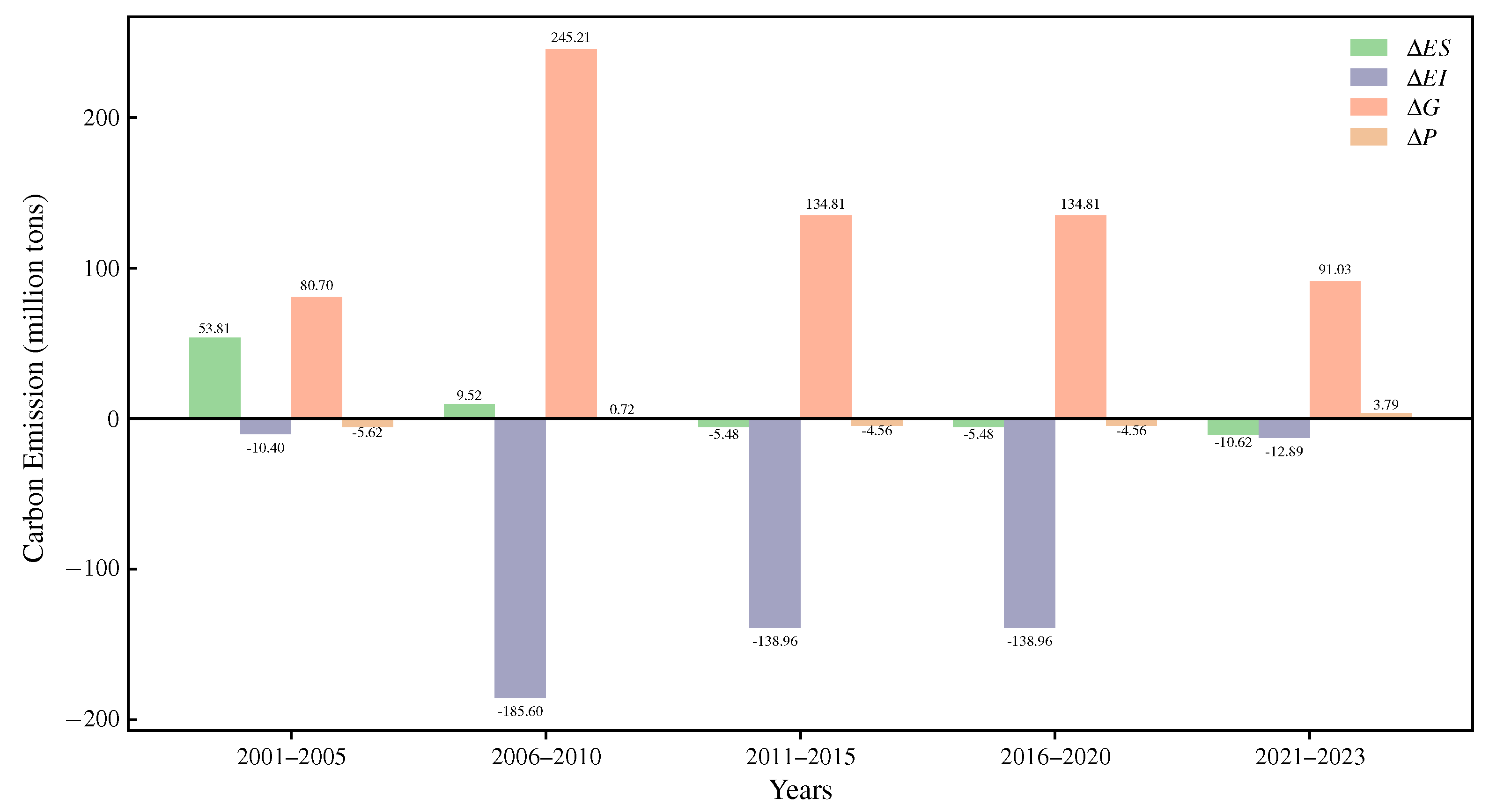
The LMDI model was applied to examine carbon emission changes in Hubei Province from 2000 to 2023, where 2000 serves as the base year for the LMDI decomposition. Following the standard LMDI methodological framework outlined in Section 3.2, the decomposition results show that the changes in carbon emissions can be attributed to five contributing factors: carbon emission factor (F), energy structure (ES), energy intensity (EI), GDP per capita (G), and population size (P). The decomposition of carbon emissions was conducted, and the results indicated that they could be attributed to five factors. Because the carbon emission coefficients remain basically unchanged, is set to 0 in this paper. Figure 4 shows the contribution of each influencing factor.
Figure 4.
LMDI cumulative graph by stages.
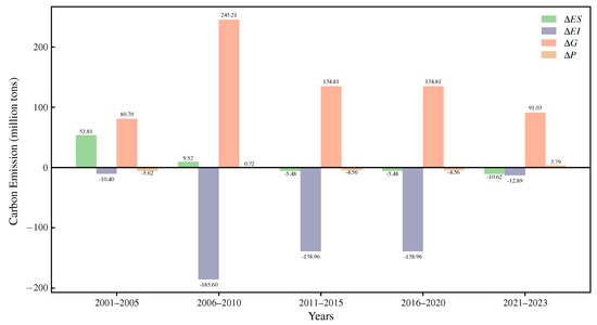
As demonstrated in Figure 4, it is evident that economic growth has consistently served as the predominant driver of carbon emissions, contributing the most substantial positive increments across all periods, particularly from 2006 to 2010, with a peak contribution of 245.21 million tons. In contrast, the energy intensity exhibited a substantial mitigating effect, particularly during the period between 2006 and 2010, and once more from 2011 to 2020. During these periods, there were reductions in excess of 185 million tons and 138 million tons, respectively. The findings of this study indicate that enhancements in energy efficiency have been instrumental in counterbalancing emissions resulting from economic growth.
The energy structure and population exhibited relatively minor and fluctuating impacts. Initially positive, the contribution of energy structure turned negative in later periods, reflecting a gradual shift towards cleaner energy sources. The impact of population growth on emission trends was negligible, indicating that economic growth and energy intensity exert a stronger influence.
Overall, the results highlight that while economic growth significantly amplifies carbon emissions, improvements in energy intensity serve as a crucial counterbalance. Transitioning to cleaner energy and controlling energy consumption per unit of GDP remain vital strategies for sustainable development in Hubei Province.
4.3. Performance of the Prediction Models
4.3.1. The Result of GA-BP
In the GA-BP model, the inputs are seven influencing factors and the output is carbon emissions. The number of neurons in the hidden layer is determined using an empirical formula and set to 9, meaning the neural network structure of this paper is (7, 9, 1).
where l represents the number of nodes in the hidden layer, n represents the number of nodes in the input layer, m represents the number of nodes in the output layer, and a is a constant ().
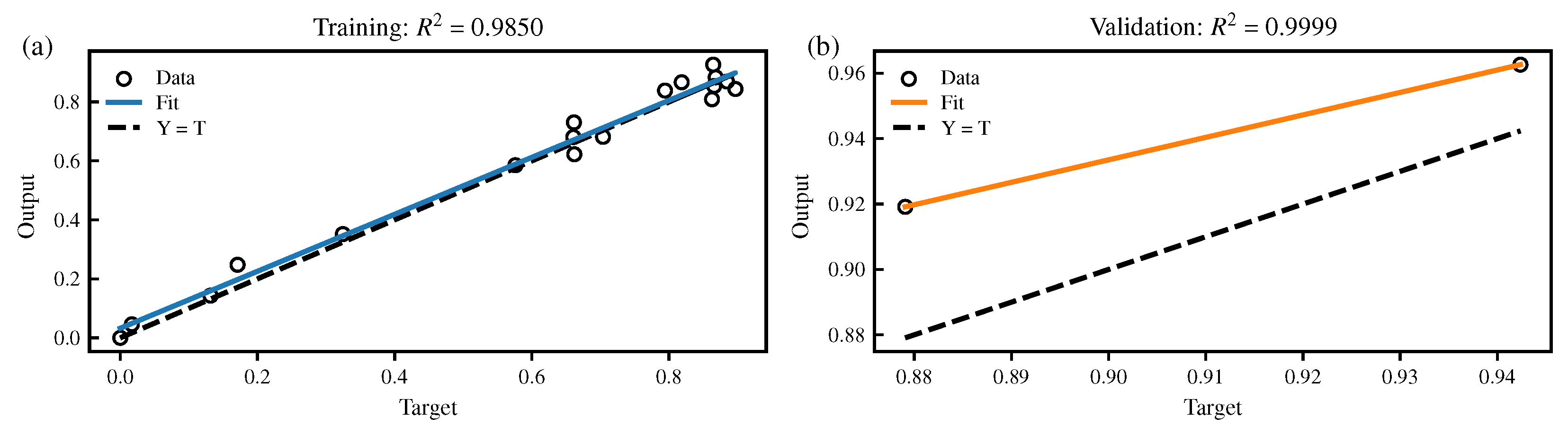
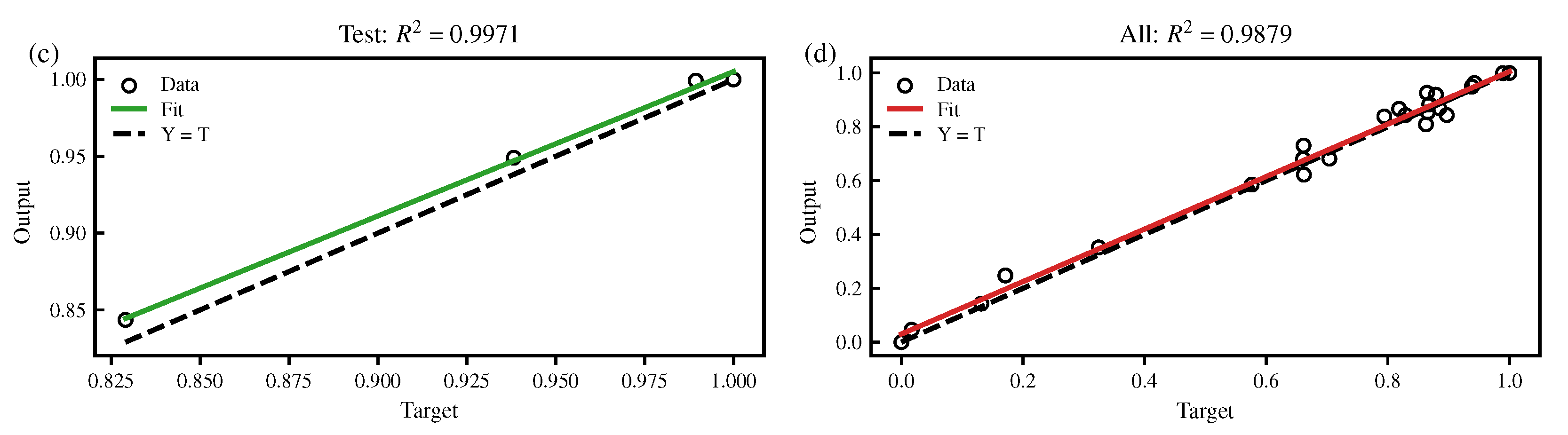
The data from 2000 to 2017 are selected as the training set, 2018 to 2019 as the validation set and 2020 to 2023 as the test set and the training set will be randomly disrupted. The parameters of the GA have been set as follows: the population size is 200, the maximum number of genetic generations is 800, the exchange probability is 0.8, and the mutation probability is 0.2. And the parameters of the BP network have been set as follows: the learning rate is and the epoch is 2000, and using early stops to avoid missing the best models, the excitation function is set to “Sigmoid” (). The training result is shown in Figure 5.
Figure 5.
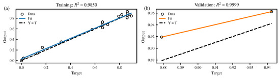
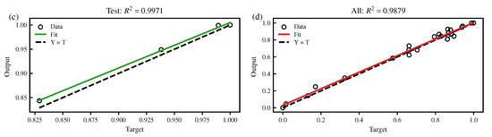
The result of GA-BP training. (a) Training set, (b) Validation set, (c) Test set, (d) All data. In each subfigure, the solid line represents predicted values, and the dashed line represents actual values.
As demonstrated in Figure 5, the of the model on the test set is 0.9971, and the fitting line is also closer to the ideal line, indicating that the model has a good generalization ability for unseen data. On the overall dataset, the model’s is 0.9897 with an intercept close to 0 and a uniform scatter distribution, reflecting the overall stability of the model. The model demonstrated a high degree of correlation () across the training, validation, and test sets, signifying its effective capacity for fitting and generalization.
4.3.2. Sensitivity Analysis of the GA-BP Model
In this study, two complementary methods were employed to evaluate model sensitivity in the GA-BP carbon emission prediction model: One-at-a-Time (OAT) local sensitivity analysis and permutation importance. OAT sensitivity analysis systematically perturbs each input variable individually (±20% in this study) while keeping other variables fixed at their baseline values. The resulting changes in model output () are used to calculate sensitivity coefficients (Si) and normalized sensitivities (Snorm). This approach provides a direct, intuitive measure of how small changes in each feature affect the model’s predicted carbon emissions, including the directionality of the effect. Permutation importance, on the other hand, evaluates the global contribution of each feature to the model’s predictive performance. By randomly shuffling one feature at a time across the dataset and measuring the increase in prediction error (MSE), this method captures both nonlinear and interaction effects among features. The results are shown in Table 3.
Table 3.
Feature sensitivity analysis results using OAT and permutation importance.
As demonstrated in Table 3, the sensitivity of each input feature on predicted carbon emissions was evaluated using two complementary approaches: OAT local sensitivity analysis and permutation importance. The changes in predicted emissions (), sensitivity coefficients (), and normalized sensitivities () for each feature are summarized in the table. Notably, TIEV and per capita GDP (G) exhibit the highest normalized sensitivities ( and 0.503, respectively), indicating that small local perturbations in these variables significantly influence model outputs. In contrast, features such as resident population (P) and energy intensity (EI) display low values (), suggesting a minor local impact on predicted emissions. The sign of further reveals the directionality of the effect: for instance, increases in TIEV and G lead to higher predicted emissions, whereas increases in EI and P slightly reduce emissions.
The permutation importance of each feature, which quantifies the contribution of each feature to the overall predictive performance of the GA-BP model, is also reported in the table. Consistent with the OAT results, TIEV and G exhibit the highest importance (0.000585 and 0.000164), confirming their critical roles in maintaining model accuracy. Features such as P and EI show negligible permutation importance, indicating that, while they may have nonzero OAT sensitivities, their contribution to overall prediction accuracy is limited.
In addition to feature sensitivity, the stability of the GA-BP model was evaluated through repeated training and prediction experiments. The OAT analysis shows that model outputs respond predictably and smoothly to input perturbations, without extreme fluctuations, indicating local robustness.
4.3.3. Comparison of Generalization Ability of Models
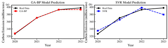
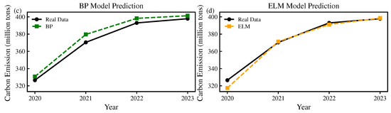
The model’s ability to generalize was used to predict carbon emissions for the period 2020–2023, with ELM, SVR, BP, and GA-BP being employed to illustrate the GA-BP model’s predictive accuracy. To evaluate the performance of different models in carbon emission prediction, four models were compared using three common evaluation metrics: the mean absolute percentage error (MAPE), the root mean square error (RMSE), and the coefficient of determination (R2). For the input variables, output variables, and sample data of the three models (ELM, SVR, and BP), the dataset division is consistent with that of GA-BP, and the parameter optimization method uses the grid search method. Among them, the structure of the BP neural network is consistent with that of the GA-BP model.
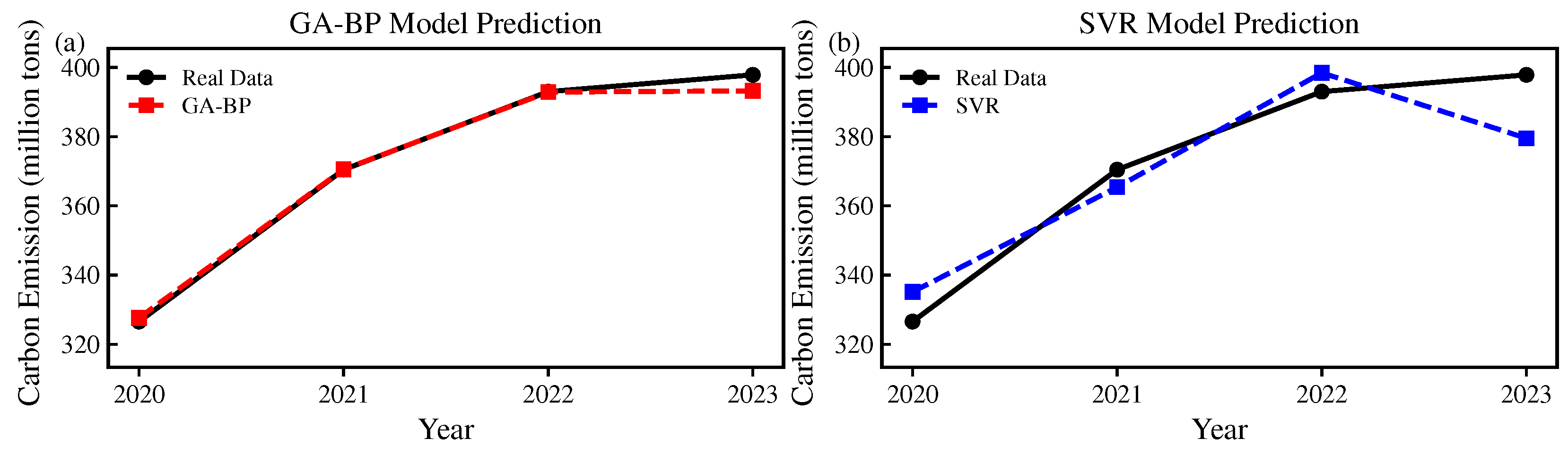
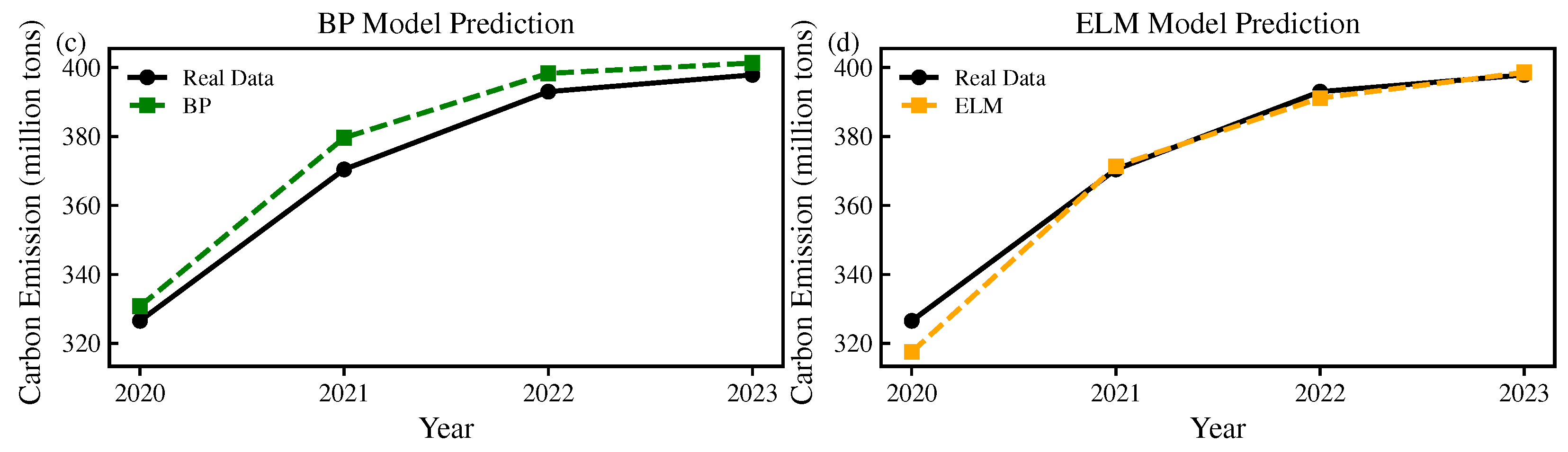
As shown in Table 4 and Figure 6, the results show that the GA-BP model achieved the best overall performance, with the lowest MAPE of 0.389%, an RMSE of 2.379, and a high R2 value of 0.993, indicating excellent predictive accuracy and consistency with the actual values. Both the standard BP neural network and the ELM model also exhibited good performance, with R2 values of 0.955 and 0.973, respectively, though their prediction errors were slightly higher than that of GA-BP. In contrast, the SVR model performed relatively poorly, with a MAPE of 2.494%, an RMSE of 10.771, and an R2 of only 0.854, suggesting limited fitting ability on this dataset. These findings highlight that incorporating a genetic algorithm to optimize the weights and thresholds of the BP network significantly enhances the model’s prediction accuracy and generalization ability. Therefore, the GA-BP model demonstrated superior predictive performance in this study and can be considered the most suitable approach for carbon emission forecasting.
Table 4.
Error indicators of four models.
Figure 6.
Comparison of the model. (a) GA-BP model prediction, (b) SVR model prediction, (c) BP model prediction, (d) ELM model Prediction. In each panel, the solid line represents actual values and the dashed line represents predicted values.
4.4. Scenario Analysis
4.4.1. Scenario Setting
The scenario of the paper mainly predicts the carbon emissions of Hubei Province from 2024 to 2035 and divides the period from 2024 to 2035 into three stages according to China’s national conditions: the 14th Five-Year Plan period from 2024 to 2025, the 15th Five-Year Plan period from 2026 to 2030, and the 16th Five-Year Plan period from 2031 to 2035. In this paper, the influencing factors are categorized into three development speeds, high, medium and low, and six scenarios are set up, according to the development plan of Hubei Province. The specific settings are shown in the Table 5.
Table 5.
Scenario setting table.
- (1)
- Population (P)
According to the Hubei Provincial Population Development Plan [34], the Hubei Province population development situation shows the long-term stability of the low fertility level, the population growth rate continues to decline, the population size tends to be stable and peaks, and based on the sixth census data, it is expected that the total population of the province will reach the peak of 60.9 million in 2028–2030. This paper assumes that the population of Hubei Province will reach a peak of 60.9 million in 2030, an increase of 2.46 million compared with 58.44 million in 2022, with an increment of 4.2%. Under the medium scenario, the growth rate of three periods is set as follows: 0.75% in the first stage, 0.55% in the second stage, and −0.20% in the third stage. In the high-carbon and low-carbon scenarios, the population change in the first and second phases is the same as the medium scenario, and in the third phase, the high scenario is set at −0.22% and the low scenario is set at −0.15%. The specific values are shown in Table 6.
Table 6.
Population scenario table.
- (2)
- Urbanization Rate (U)
In the 14th Five-Year Plan for National Economic and Social Development of Hubei Province and the outline of the 2035th Five-Year Plan (hereinafter referred to as the “14th Five-Year Plan”) [35], it is mentioned that the urbanization rate of Hubei Province will reach 65% in 2025, with an increase of 3.6%, so the growth rate of the three time periods under the baseline scenario is set as follows: In the first phase, the growth rate was 0.80%; in the second phase, 0.60%; and in the third phase, 0.40%. An increase of 0.2% in each phase is a high scenario, and a decrease of 0.2% is a low scenario. The specific values are shown in Table 7.
Table 7.
Urbanization rate scenario table.
- (3)
- Total import and export trade/GDP (TIEV)
In the 14th Five-Year Plan for the proportion of import and export trade volume in Hubei Province, it does include direct planning. This paper will be set according to the average growth rate of the proportion of import and export trade volume in the 13th Five-Year Plan period (2016–2020) and the 14th Five-Year Plan period. In the 13th Five-Year Plan period, the average growth rate of the proportion of import and export trade volume in Hubei Province is 0.464%, while the average growth rate in 2021–2023 is 0.43%. Under comprehensive consideration, the growth rate of TIEV in this paper is 0.45% in the first stage of the medium scenario, 0.35% in the second stage, and 0.25% in the third stage. An increase of 0.1% in each phase is a high scenario, and a decrease of 0.1% is a low scenario. The specific values are shown in Table 8.
Table 8.
TIEV scenario table.
- (4)
- GDP per Capita (G)
In the “14th Five-Year Plan” [35], the annual growth rate of regional GDP in the future is expected to be about 6.5%, and the transformation of epidemic prevention and control policy has created good conditions for Hubei’s economic recovery. In this paper, the growth rate of the three time periods under the baseline scenario is set as follows: In the first phase, the growth rate is 6.0%; in the second phase, 7.0%; and in the third phase, 8.0%. An increase of 1.0% in each phase is a high-carbon scenario, and a decrease of 1.0% is a low-carbon scenario. The specific values are shown in Table 9.
Table 9.
GDP per capita scenario table.
- (5)
- Industrial Structure (IS)
Through analyzing the data of industrial structure during 2015–2020, it is found that during the “13th Five-Year Plan” period, the industrial structure of Hubei Province declined by 8.87%, with an average annual decline of 2.7%. However, there will be a rebound in 2021–2022. Under comprehensive consideration, the growth rate of the three time periods under the benchmark scenario is set as follows: The growth rate in the first stage is −1.9%, the growth rate in the second stage is −1.8%, and the growth rate in the third stage is −1.7%. A 0.3% increase in each phase is a high scenario, and a 0.3% decrease is a low scenario. The specific values are shown in Table 10.
Table 10.
Industrial structure scenario table.
- (6)
- Energy Intensity (EI)
According to the “14th Five-Year Plan” for energy development in Hubei Province [36], the energy intensity of Hubei Province during the 14th Five-Year Plan period has been reduced by 14%, with an average annual reduction of 2.8%. Therefore, the growth rate of the three periods under the benchmark scenario is set as follows: the growth rate of the first stage is −2.4%, the growth rate of the second stage is −2.5%, and the third stage is −2.6%. A 0.3% increase in each phase is a high scenario, and a 0.3% decrease is a low scenario. The specific values are shown in Table 11.
Table 11.
Energy intensity scenario table.
- (7)
- Energy Structure (ES)
According to the “14th Five-Year Plan” for energy development in Hubei Province [36], the proportion of coal consumption has declined by 2.5%, with an average annual decline of 0.5%, so this paper sets the growth rate of the three time periods under the benchmark scenario, respectively, as follows: the growth rate of the first stage −0.10%, the growth rate of the second stage −1.20 %, and the third stage −1.40%. An increase of 0.40% in each phase is a high scenario, and a decrease of 0.40% is a low scenario. The specific values are shown in Table 12.
Table 12.
Energy structure scenario table.
4.4.2. Scenario Analysis Result
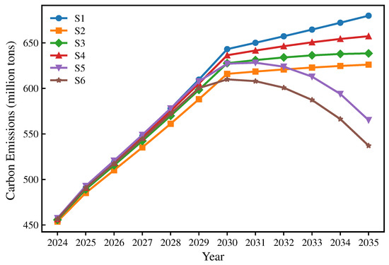
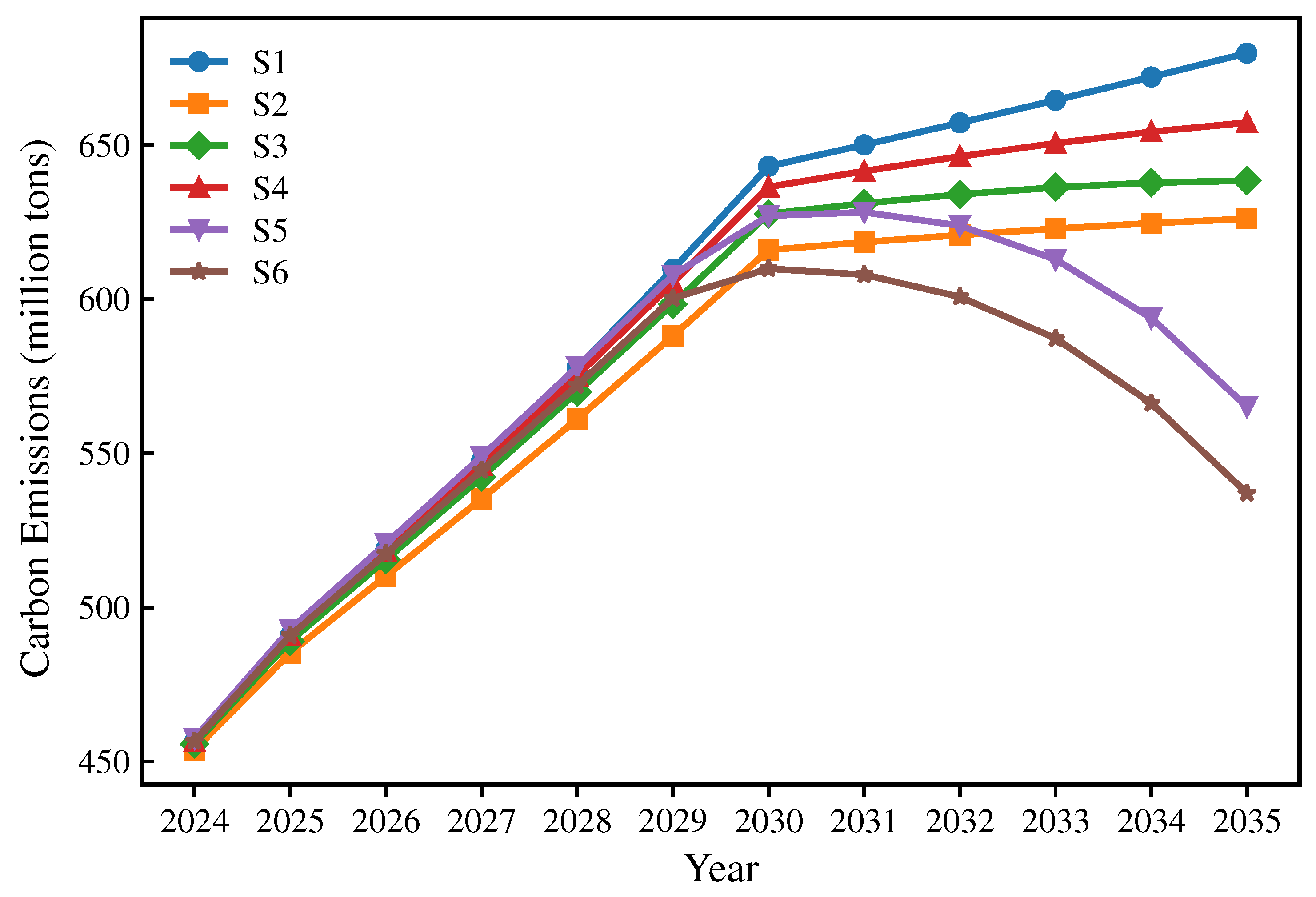
Based on the GA-BP model, the carbon emission peak and the carbon peak time of Hubei Province from 2024 to 2035 were predicted according to six scenarios. The forecast results of carbon emissions in Hubei Province in 2025–2035 under various scenarios are shown in Table 13 and Figure 7. According to the prediction results of the GA-BP model, the peak value and peak time of carbon emissions in Hubei Province are different under different scenarios, and the peak time of carbon emissions in different development paths is also different under different scenarios.
Table 13.
Forecasting results of C in different scenarios.
Figure 7.
Scenario prediction.
Based on Table 13 and Figure 7, from the carbon emission projection results of each scenario, it can be seen that none of the S1–S4 scenarios peaks before 2030, and the carbon emission shows a continuous upward trend. Among them, the S1 scenario has the highest peak at 679.87 million tons, and the S5 scenario peaks at 628.22 million tons in 2031, which is later than 2030 but slightly lower than the emission levels of S1-S4. The only scenario that achieves peak carbon by 2030 is S6, which peaks at 6,09.92 million tons in 2030, with the lowest emissions of all the scenarios, suggesting that this scenario has stronger emission reduction and policy intervention effects. Overall, only the S6 scenario achieves the “peak by 2030” target, indicating that it has a significant advantage in the low-carbon transition pathway, while the remaining scenarios require stronger mitigation measures to achieve the dual-carbon target.
5. Discussion
5.1. Comparison of Results from LMDI, STIRPAT-Lasso, and OAT Sensitivity Analysis
In this study, we employed three complementary approaches—LMDI decomposition, STIRPAT-Lasso feature selection, and OAT sensitivity analysis—to identify and quantify the key drivers of carbon emissions in Hubei Province. Interestingly, the results vary across methods. Both the LMDI and STIRPAT-Lasso consistently identify per capita GDP (G) and energy intensity (EI) as the most significant factors, whereas the OAT analysis highlights trade intensity (TIEV) alongside per capita GDP (G) as the most influential. This methodological combination enables a comprehensive assessment that captures both long-term structural effects and short-term local variations. Overall, per capita GDP emerges as the dominant driver, while other factors—including trade intensity, energy intensity, energy structure, urbanization rate, and resident population—play secondary or moderating roles. In the following sections, we systematically compare the outcomes of these methods, examine the reasons for consistencies and discrepancies, and discuss their implications for regional carbon reduction strategies.
The consistency between the LMDI and STIRPAT-Lasso results can be attributed to their focus on long-term structural relationships between carbon emissions and socio-economic factors. Both methods capture cumulative contributions over time, with STIRPAT-Lasso additionally controlling for multicollinearity and highlighting the statistically robust drivers. Consequently, per capita GDP (G) and energy intensity (EI) emerge as the dominant factors in both approaches. In contrast, OAT evaluates the local sensitivity of emissions to one variable at a time, emphasizing short-term perturbations rather than cumulative long-term effects. As a result, trade intensity (TIEV) appears more influential in the OAT analysis, reflecting its higher short-term volatility and immediate impact on carbon emissions, even though its long-term structural contribution is comparatively minor. This distinction highlights the complementary nature of these methods, providing both a structural perspective and a local, short-term sensitivity perspective on Hubei’s carbon emission drivers.
Overall, the results consistently recognize per capita GDP (G) as the most significant driver of carbon emissions in Hubei Province, highlighting the strong coupling between economic growth and energy consumption. From a policy perspective, this underscores the need to promote low-carbon economic development, improve energy efficiency, and encourage structural upgrading of the industrial sector to decouple economic growth from carbon emissions. The observed differences across methods also provide valuable policy insights: While the LMDI and STIRPAT–Lasso emphasize long-term structural effects, the OAT results highlight the short-term sensitivity of emissions to trade intensity (TIEV). This suggests that in addition to long-term strategies focusing on economic and industrial transformation, policymakers should also consider short-term interventions targeting trade-related emissions fluctuations, such as optimizing import–export structures, enhancing clean production in trade-intensive industries, and promoting low-carbon logistics. Integrating these perspectives allows for both immediate and sustainable carbon reduction strategies tailored to Hubei Province’s unique economic and energy profile.
5.2. Analysis of Carbon Reduction Pathways
Based on the scenario analysis presented in Table 5 and Table 13, it is evident that Hubei Province can achieve carbon peaking by 2030 only under scenario 6, which corresponds to low levels of population (P), urbanization rate (U), and per capita GDP (G), combined with high energy intensity (EI) and energy structure (ES) improvements. In contrast, under scenarios S1–S5, carbon emissions either continue to rise beyond 2030 or reach the peak shortly thereafter, indicating that current socio-economic growth trajectories and energy policies are insufficient for timely carbon peaking. This comparison highlights the critical role of coordinated socio-economic and energy policy interventions in shaping carbon emission pathways. In the following discussion, we analyze the implications of each scenario for low-carbon development strategies, identify key leverage points for emission reductions, and provide recommendations for policy measures tailored to Hubei Province’s industrial and energy profile.
The scenario analysis highlights distinct carbon emission trajectories across the six examined pathways, providing insights into effective reduction strategies for Hubei Province. Based on the carbon peaking outcomes, the scenarios are divided into three groups: S1–S4, in which carbon emissions continue to rise; S5, in which carbon peaking is achieved but occurs later than 2030; and S6, in which the carbon peaking target is successfully met. Under scenarios S1–S4, which combine high or medium socio-economic growth with limited energy and industrial adjustments, emissions continue to rise beyond 2030 or peak only slightly later. This indicates that high population, urbanization, and per capita GDP, without sufficient improvements in energy structure and efficiency, are insufficient to achieve timely carbon peaking. Policy measures for these scenarios should focus on accelerating the transition to cleaner energy, enhancing energy efficiency across industries, and guiding urbanization and population growth toward low-carbon patterns. Scenario S5, representing medium socio-economic growth with partial energy and industrial adjustments, results in emissions peaking shortly after 2030, demonstrating that moderate interventions can moderately curb emissions but are insufficient for on-time peaking. Targeted measures in this scenario include optimizing the energy mix, improving energy efficiency in trade-intensive sectors, and promoting industrial upgrading. In contrast, Scenario S6, characterized by low population and economic intensity combined with high energy efficiency and cleaner energy adoption, achieves carbon peaking by 2030 with the lowest peak value. This scenario underscores the effectiveness of coordinated socio-economic and energy interventions and provides a benchmark for low-carbon development pathways. Overall, the grouped analysis emphasizes that timely carbon peaking in Hubei requires an integrated approach combining socio-economic control, structural energy improvements, and industrial transformation, allowing policymakers to design both immediate and long-term emission reduction strategies tailored to the province’s unique economic and energy profile.
6. Conclusions and Suggestions
6.1. Conclusions
This article focuses on the carbon emissions in Hubei Province from 2000 to 2023. The LMDI method was employed to decompose historical carbon emissions using a standard set of fixed factors for diagnostic purposes. Subsequently, the STIRPAT and Lasso models were applied to evaluate a broader set of 10 potential variables, from which seven specific factors were selected as inputs for the predictive GA-BP model. The superiority and accuracy of the GA-BP prediction model were verified by verifying the fitting effect of the GA-BP model and comparing the prediction results of different models. Finally, the GA-BP model was used to predict the carbon emissions of Hubei Province from 2024 to 2035, and the carbon emission peaks under six scenarios were discussed.
The following conclusions are drawn:
(1) Per capita GDP (G) is the dominant driver of carbon emissions in Hubei Province, underscoring the strong link between economic growth and energy consumption. Effective carbon reduction requires a dual approach: long-term strategies aimed at promoting low-carbon economic development, improving energy efficiency, and upgrading industrial structures, combined with short-term interventions addressing trade-related emissions fluctuations. By integrating structural reforms with targeted short-term measures, policymakers can design sustainable and context-specific pathways to achieve carbon peaking and facilitate the province’s transition toward a low-carbon economy.
(2) This paper develops the GA-BP model using data from Hubei Province from 2000 to 2023 and conducts a comparative analysis with the ELM, SVR, and BP models. The findings demonstrate the superior performance of the GA-BP model for the dataset. The values in all dataset partitions exceeded 0.98, demonstrating strong learning and generalization capabilities. In comparison with the other models, the GA-BP model achieved the best performance in terms of the , MAPE, and RMSE, confirming its superior accuracy.
(3) Six scenarios were designed. Only two scenarios achieve the carbon peak, and only scenario S6 reaches the peak by 2030, indicating stronger emission reduction potential and policy responsiveness, representing the optimal pathway to achieving the carbon peak target. The remaining scenarios require greater emission reduction efforts to achieve the carbon peak before 2030.
6.2. Suggestions and Outlook
Based on the conclusions of calculation, decomposition, forecast, and scenario analysis of carbon emissions in Hubei Province, the paper puts forward some policy recommendations. (1) Economic development is one of the key drivers of carbon emissions in Hubei Province. With the advancement of industrialization and urbanization, the total amount of energy consumption has been rising, leading to a continuous increase in the level of carbon emissions. However, economic growth and carbon emissions are not irreconcilable conflicts. By promoting green and low-carbon technological innovation, optimizing industrial structure, and improving the efficiency of energy use, it is possible to achieve the harmonization of economic development and carbon emission reduction. In the long run, Hubei Province needs to accelerate the construction of a new development model with low carbon as the core and gradually reduce the carbon emission intensity per unit of GDP while ensuring steady economic growth. Especially in the context of the “14th Five-Year Plan” and the “Double Carbon” target, Hubei should strengthen policy guidance and institutional support, promote the transformation and upgrading of traditional high-energy-consuming industries, and encourage the development of green finance and new energy industries so as to realize the transition from “high-carbon growth” to “low-carbon growth”.
(2) Reducing energy intensity is the most effective measure for carbon mitigation, while changes in energy structure have a relatively smaller direct impact on emissions. Therefore, Hubei should prioritize energy efficiency improvements across industries, promote the concept of green development, and encourage the growth of energy-saving and environmentally friendly sectors. At the same time, adjustments to the energy structure—from fossil fuels to cleaner energy sources—should be pursued as a complementary strategy to further support sustainable carbon reduction. High-energy-consumption and high-pollution industries should be controlled or upgraded to achieve a balanced and effective low-carbon transition.
(3) In addition to long-term structural measures, short-term fluctuations in carbon emissions related to trade intensity (TIEV) should be addressed through targeted interventions. Policymakers can optimize import–export structures, encourage cleaner production practices in trade-intensive industries, and promote low-carbon logistics. By mitigating the immediate emission impacts of trade activities, Hubei Province can complement long-term energy efficiency and industrial transformation strategies, ensuring more stable progress toward carbon peaking.
Despite the comprehensive analysis conducted in this study, several limitations should be acknowledged. First, while the GA-BP model provides robust short- to medium-term carbon emission predictions, it relies on historical socio-economic and energy data and may not fully capture unexpected structural shifts, technological breakthroughs, or policy changes beyond the current dataset. Second, the scenario analysis focuses primarily on carbon peaking by 2030 and does not extend to the longer-term trajectory required for achieving carbon neutrality by 2060. Future research could integrate more advanced predictive models, such as hybrid machine learning approaches or system dynamics models, to capture complex nonlinear interactions and long-term uncertainties. Additionally, incorporating prospective policy interventions, renewable energy adoption rates, and emerging low-carbon technologies would provide a more realistic projection toward the 2060 carbon neutrality target. Addressing these aspects will enhance the model’s predictive power and provide more actionable insights for policymakers to design both near-term and long-term strategies for Hubei Province’s sustainable low-carbon transitions.
Author Contributions
Conceptualization, H.X. and D.R.; Methodology, H.X. and D.R.; Software, H.X. and D.R.; Validation, H.X. and D.R.; Formal analysis, H.X. and D.R.; Investigation, H.X. and D.R.; Resources, H.X. and D.R.; Data curation, H.X. and D.R.; Writing—original draft, H.X., D.R., Y.T., X.Z., S.Z., Y.C. and X.G.; Writing—review & editing, H.X., D.R., Y.T., X.Z., S.Z., Y.C. and X.G.; Visualization, H.X. and D.R.; Supervision, H.X., D.R., Y.T., X.Z., S.Z., Y.C. and X.G.; Project administration, H.X. and D.R.; Funding acquisition, D.R. All authors have read and agreed to the published version of the manuscript.
Funding
This work was supported by the Science and Technology Innovation Team Project of Hubei Province Department of Education (Grant No. T2020002), Wuhan Science and Technology Planning Project (Grant No. 2020020601012274), National Natural Science Foundation of China (Grant No. 41571306), and Hubei Technological Innovation Special Fund (Grant No. 2020ZYYD019).
Institutional Review Board Statement
Not applicable.
Informed Consent Statement
Not applicable.
Data Availability Statement
The data used to support the findings of this study are available from the corresponding author upon request.
Conflicts of Interest
The authors declare no conflicts of interest.
List of Abbreviations
The following abbreviations are used in this manuscript:
| BiLSTM | Bidirectional Long Short-Term Memory |
| BP | Back Propagation Neural Network |
| Bf Gas | Blast Furnace Gas |
| C | Carbon Emission |
| CNN-inceptionv2 | Convolutional Neural Network-Inception v2 |
| CO2 | Carbon Dioxide |
| CSO-FLN | Chicken Swarm Optimization-Fuzzy Logic Network |
| E | Environmental Impact |
| EI | Energy Intensity |
| ELM | Extreme Learning Machine |
| ES | Energy Structure |
| G | GDP per Capita |
| GA | Genetic Algorithm |
| GA-BP | Genetic Algorithm-Back Propagation |
| GDP | Gross Domestic Product |
| GDIM | Generalized Divisia Index Method |
| ICEEMDAN-LOBiLSTM-LOLSSVM | Improved CEEMDAN-Long- and Short-BiLSTM-Long- and Short-LSSVM |
| LMDI | Logarithmic Mean Divisia Index |
| LPG | Liquefied Petroleum Gas |
| LSTM | Long Short-Term Memory |
| MAPE | Mean Absolute Percentage Error |
| MSE | Mean Squared Error |
| NOAA | National Oceanic and Atmospheric Administration |
| P | Population |
| R2 | Coefficient of Determination |
| RMSE | Root Mean Square Error |
| SVR | Support Vector Regression |
| STIRPAT | Stochastic Impacts by Regression on Population, Affluence and Technology |
| TextCNN | Text Convolutional Neural Network |
| TIEV | The Ratio of Total Import and Export Trade Volume to the Gross Domestic Product |
Appendix A. The Result of STIRPAT Model and Lasso Model
Appendix A.1. The Extended STIRPAT Model
The STIRPAT model is improved from the IPAT model, and its basic expression is as follows:
where I represents the environmental impact or environmental pressure; P represents the population factor; A represents the economic factor; T represents the technological factor; a is the model coefficient; b, c, and d are the indices of each influencing factor; and e is the error term. For the convenience of estimation and verification, the STIRPAT model is generally transformed into logarithmic form.
In order to accurately predict carbon emissions, this paper selects 10 indicators as variables and adds them to the STIRPAT model, as shown below:
where C is the carbon emission; the meaning of Xi(i = 1,2,3,…,10) is shown in Table A1.
Table A1.
Description of influencing factors.
Appendix A.2. Lasso Model
Lasso regression is mainly used to solve the problem of data modeling with high-dimensional features, and at the same time, feature selection and regularization are carried out to improve the predictive ability and explanatory ability of the model. Lasso regression adds the L1 norm penalty term to the loss function of linear regression, and its objective function is as follows:
where represents the response variable for the response variable for the i observation, is the value of the jth predictor variable for the i-th sample j value of the predictor variable, is the corresponding regression coefficient, is the intercept term, and is a non-negative regularization parameter that controls the degree of coefficient shrinkage and model sparsity.
Appendix A.3. The Result of STIRPAT Model
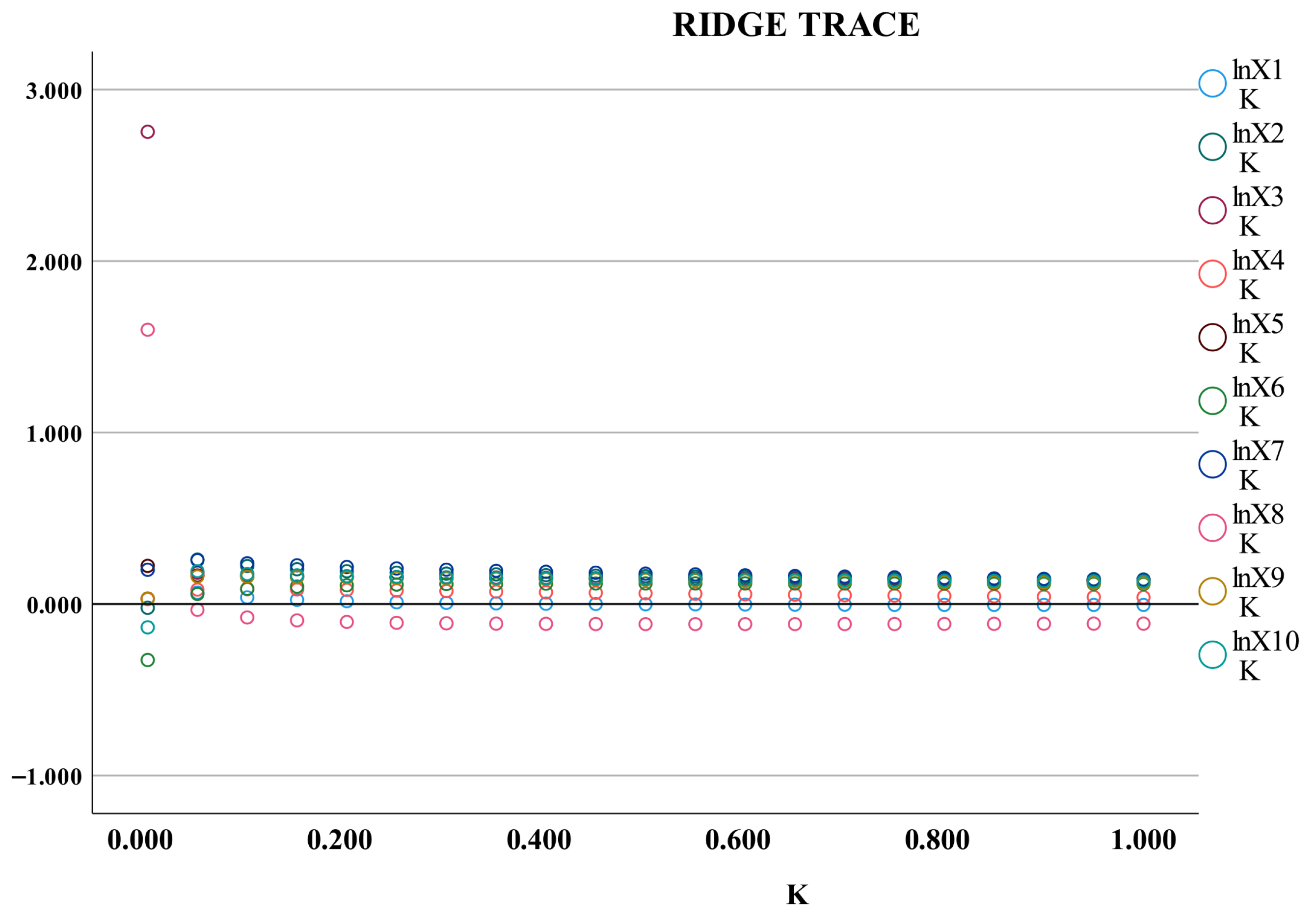
In this paper, a linear regression analysis of STIRPAT was conducted using SPSS27, and the analysis results are shown. It can be seen from the linear regression result table that except for the VIF of X4 and X9 being less than 10, the other factors are greater than 10, and the maximum VIF is 1249.702 of the X3 factor. The VIF analysis shows that there is a highly correlated relationship between explanatory variables. In order to reduce the generalization error caused by multicollinearity and improve the accuracy and stability of the model, ridge regression will be used in this paper to fit the model.
Table A2.
The result of STIRPAT linear regression.
Ridge regression is a biased estimation method derived by the least square method, which makes the coefficient more stable by correction. When the independent variables in the model have a strong collinear relationship, the linear model will be very unstable. In this case, ridge regression analysis can be used to solve the above problems.
As shown in Figure A1, all coefficients tend to be stable when K = 0.15, so K = 0.15 is taken as the hyperparameter of the ridge regression.
Figure A1.
Ridge regression result.
Appendix A.4. The Result of Lasso Model
In this paper, the Lasso model is constructed using Python 3.11.5, and the result of the STIRPAT model is taken as the initial estimation value of the Lasso model. The specific results are shown in the Figure A2 and Table A3.
Figure A2.
The result of the Lasso model.
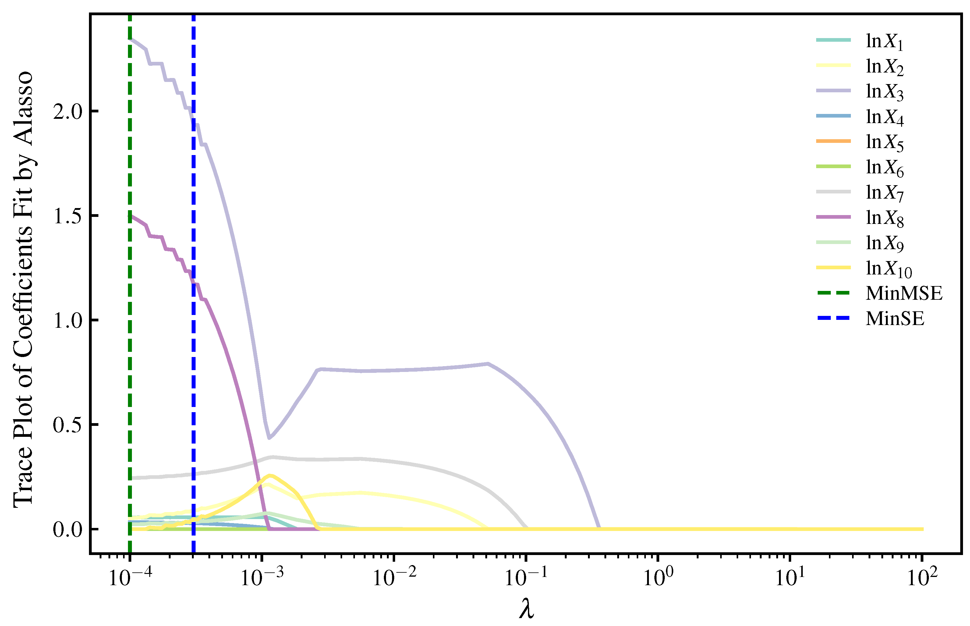
As shown in Table A3, a total of seven significant influencing factors were screened out by the Lasso model. The minimum mean square error (MSE) is 0.0112%, and the fitting effect is very good.
Table A3.
Result of the Lasso model.
References
- Lan, X.; Tans, P.; Thoning, K.W. Trends in Globally-Averaged CO2 Determined from NOAA Global Monitoring Laboratory Measurements; NOAA Global Monitoring Laboratory: Boulder, CO, USA, 2025. [Google Scholar] [CrossRef]
- Zhao, Y.; Liu, R.; Liu, Z.; Liu, L.; Wang, J.; Liu, W. A Review of Macroscopic Carbon Emission Prediction Model Based on Machine Learning. Sustainability 2023, 15, 6876. [Google Scholar] [CrossRef] [Scilit]
- Zheng, Y.; Shan, R.; Xu, W.A.; Qiu, Y.L. Effectiveness of Carbon Dioxide Emission Target Is Linked to Country Ambition and Education Level. Commun. Earth Environ. 2024, 5, 1–11. [Google Scholar] [CrossRef] [Scilit]
- Liu, Z.; Guan, D.; Moore, S.; Lee, H.; Su, J.; Zhang, Q. Climate policy: Steps to China’s carbon peak. Nature 2015, 522, 279–281. [Google Scholar] [CrossRef] [Scilit]
- The Central Committee of the Communist Party of China; The State Council of the People’s Republic of China. Opinions on Fully, Accurately, and Comprehensively Implementing New Development Concepts to Achieve Carbon Peaking and Carbon Neutrality; State Council of the People’s Republic of China: Beijing, China, 2021. [Google Scholar]
- Ziyuan, C.; Yibo, Y.; Simayi, Z.; Shengtian, Y.; Abulimiti, M.; Yuqing, W. Carbon emissions index decomposition and carbon emissions prediction in Xinjiang from the perspective of population-related factors, based on the combination of STIRPAT model and neural network. Environ. Sci. Pollut. Res. 2022, 29, 31781–31796. [Google Scholar] [CrossRef] [Scilit]
- Lu, F.; Ma, F.; Feng, L. Carbon Dioxide Emissions and Economic Growth: New Evidence from GDP Forecasting. Technol. Forecast. Soc. Change 2024, 205, 123464. [Google Scholar] [CrossRef] [Scilit]
- Tang, J.; Zheng, J.; Yang, G.; Li, C.; Zhao, X. Carbon Emission Prediction in a Region of Hainan Province Based on Improved STIRPAT Model. Environ. Sci. Pollut. Res. 2024, 31, 58795–58817. [Google Scholar] [CrossRef] [Scilit] [PubMed]
- Suo, R.; Wang, Q.; Han, Q. Driver Analysis and Integrated Prediction of Carbon Emissions in China Using Machine Learning Models and Empirical Mode Decomposition. Mathematics 2024, 12, 2169. [Google Scholar] [CrossRef] [Scilit]
- Hou, K.; Sun, J.; Dong, M.; Zhang, H.; Li, Q. Simulation of Carbon Peaking Process of High Energy Consuming Manufacturing Industry in Shaanxi Province: A Hybrid Model Based on LMDI and TentSSA-ENN. Math. Biosci. Eng. 2023, 20, 18445–18467. [Google Scholar] [CrossRef] [Scilit] [PubMed]
- Chen, L.; Ma, M.; Xiang, X. Decarbonizing or Illusion? How Carbon Emissions of Commercial Building Operations Change Worldwide. Sustain. Cities Soc. 2023, 96, 104654. [Google Scholar] [CrossRef] [Scilit]
- Rao, Y.; Wang, X.; Li, H.; Ruan, Y. How can the Pearl River Delta urban agglomeration achieve the carbon peak target: Based on the perspective of an optimal stable economic growth path. J. Clean. Prod. 2024, 439, 140879. [Google Scholar] [CrossRef] [Scilit]
- Yu, Y.; Du, Y. Impact of technological innovation on CO2 emissions and emissions trend prediction on ’New Normal’ economy in China. Atmos. Pollut. Res. 2019, 10, 152–161. [Google Scholar] [CrossRef] [Scilit]
- Chen, X.; Shuai, C.; Wu, Y.; Zhang, Y. Analysis on the Carbon Emission Peaks of China’s Industrial, Building, Transport, and Agricultural Sectors. Sci. Total Environ. 2020, 709, 135768. [Google Scholar] [CrossRef] [Scilit]
- Lin, C.; Li, X. Carbon peak prediction and emission reduction pathways exploration for provincial residential buildings: Evidence from Fujian Province. Sustain. Cities Soc. 2024, 102, 105239. [Google Scholar] [CrossRef] [Scilit]
- Zhao, Y.; Su, Q.; Li, B.; Zhang, Y.; Wang, X.; Zhao, H.; Guo, S. Have those countries declaring “zero carbon” or “carbon neutral” climate goals achieved carbon emissions-economic growth decoupling? J. Clean. Prod. 2022, 363, 132450. [Google Scholar] [CrossRef] [Scilit]
- Jin, Y.; Sharifi, A.; Li, Z.; Chen, S.; Zeng, S.; Zhao, S. Carbon emission prediction models: A review. Sci. Total Environ. 2024, 927, 172319. [Google Scholar] [CrossRef] [Scilit]
- Ren, F.; Long, D. Carbon emission forecasting and scenario analysis in Guangdong Province based on optimized Fast Learning Network. J. Clean. Prod. 2021, 317. [Google Scholar] [CrossRef] [Scilit]
- Shi, C.; Zhi, J.; Yao, X.; Zhang, H.; Yu, Y.; Zeng, Q.; Li, L.; Zhang, Y. How can China achieve the 2030 carbon peak goal-a crossover analysis based on low-carbon economics and deep learning. Energy 2023, 269, 126776. [Google Scholar] [CrossRef] [Scilit]
- Li, Y.; Wang, Z.; Liu, S. Enhance Carbon Emission Prediction Using Bidirectional Long Short-Term Memory Model Based on Text-Based and Data-Driven Multimodal Information Fusion. J. Clean. Prod. 2024, 471, 143301. [Google Scholar] [CrossRef] [Scilit]
- Li, G.; Wu, H.; Yang, H. A Multi-Factor Combination Prediction Model of Carbon Emissions Based on Improved CEEMDAN. Environ. Sci. Pollut. Res. 2024, 31, 20898–20924. [Google Scholar] [CrossRef] [Scilit]
- National Bureau of Statistics of China; Hubei Provincial Team. Summary of Key Findings from the Seventh National Population Census of Hubei Province; Hubei Provincial Bureau of Statistics: Wuhan, China, 2021. [Google Scholar]
- Intergovernmental Panel on Climate Change (IPCC). Revised 1996 IPCC Guidelines for National Greenhouse Gas Inventories; Technical Report 4; IPCC Secretariat: Geneva, Switzerland, 2006. [Google Scholar]
- National Development and Reform Commission (NDRC Office). Notice on the Issuance of the Pilot Implementation Guidelines for Greenhouse Gas Emission Accounting and Reporting of the Third Batch of 10 Industries; Technical Report; National Development and Reform Commission: Beijing, China, 2021. [Google Scholar]
- Ministry of Ecology and Environment (MEE). Guidelines for Provincial-Level Greenhouse Gas Inventories (Pilot Implementation); Technical Report; (MEE Circular [2020] No. 15); Ministry of Ecology and Environment of the People’s Republic of China: Beijing, China, 2020. [Google Scholar]
- Ang, B. The LMDI approach to decomposition analysis: A practical guide. Energy Policy 2005, 33, 867–871. [Google Scholar] [CrossRef] [Scilit]
- Goh, T.; Ang, B.W. Tracking economy-wide energy efficiency using LMDI: Approach and practices. Energy Effic. 2018, 12, 829–847. [Google Scholar] [CrossRef] [Scilit]
- Dietz, T.; Rosa, E.A. Effects of population and affluence on CO2 emissions. Proc. Natl. Acad. Sci. USA 1997, 94, 175–179. [Google Scholar] [CrossRef] [Scilit]
- Zou, H. The Adaptive Lasso and Its Oracle Properties. J. Am. Stat. Assoc. 2006, 101, 1418–1429. [Google Scholar] [CrossRef] [Scilit]
- Ameyaw, B.; Li, Y.; Annan, A.; Agyeman, J.K. West Africa’s CO2 emissions: Investigating the economic indicators, forecasting, and proposing pathways to reduce carbon emission levels. Environ. Sci. Pollut. Res. 2020, 27, 13276–13300. [Google Scholar] [CrossRef] [Scilit] [PubMed]
- Yang, J.; Hu, Y.; Zhang, K.; Wu, Y. An improved evolution algorithm using population competition genetic algorithm and self-correction BP neural network based on fitness landscape. Soft Comput. 2021, 25, 1751–1776. [Google Scholar] [CrossRef] [Scilit]
- National Development and Reform Commission of the People’s Republic of China. The 10th Five-Year Plan for National Economic and Social Development of the People’s Republic of China (2001–2005); National Development and Reform Commission: Beijing, China, 2001. [Google Scholar]
- Zhao, M.; Niu, Y.; Tian, L.; Liu, Y.; Zhai, Q. Impact Measurement of COVID-19 Lockdown on China’s Electricity-Carbon Nexus. Int. J. Environ. Res. Public Health 2021, 18, 9736. [Google Scholar] [CrossRef] [Scilit] [PubMed]
- People’s Government of Hubei Province. Hubei Provincial Population Development Plan (2018–2030); Government Notice No. [2018]48; People’s Government of Hubei Province: Wuhan, China, 2018. [Google Scholar]
- People’s Government of Hubei Province. Hubei Provincial 14th Five-Year Plan for National Economic and Social Development and Long-Range Objectives through the Year 2035; Government Notice, 2021; People’s Government of Hubei Province: Wuhan, China, 2021.
- People’s Government of Hubei Province. Hubei Provincial Energy Development Plan for the 14th Five-Year Plan Period (2021–2025); People’s Government of Hubei Province: Wuhan, China, 2022. [Google Scholar]

Disclaimer/Publisher’s Note: The statements, opinions and data contained in all publications are solely those of the individual author(s) and contributor(s) and not of MDPI and/or the editor(s). MDPI and/or the editor(s) disclaim responsibility for any injury to people or property resulting from any ideas, methods, instructions or products referred to in the content. |
© 2025 by the authors. Licensee MDPI, Basel, Switzerland. This article is an open access article distributed under the terms and conditions of the Creative Commons Attribution (CC BY) license.