


Abstract
In recent years, the frequent occurrence of extreme weather events has prompted increased global attention to greenhouse gas emissions. This study analyzes the spatio-temporal evolution of carbon emission intensity (CEI) across land use types in China’s 30 provinces from 2009 to 2022. Based on the data from China Rural Statistical Yearbook, China City Statistical Yearbook, China Energy Statistical Yearbook, China Natural Resources Statistical Yearbook, and China Statistical Yearbook, this study aims to reveal the spatio-temporal differentiation patterns of CEI, analyze the decoupling status between development mode and carbon emissions, and establish a three-dimensional collaborative emission reduction framework. Firstly, employing the carbon emission factor method, provincial carbon emissions, sinks, and net emissions are calculated, with intensity levels derived from gross domestic product (GDP). Secondly, spatio-temporal trends and inter-provincial disparities are analyzed using the decoupling index. The spatial effects among the provinces are investigated based on Moran’s I index. The results show that while the overall CEI has declined since 2009, significant regional disparities persist, with the southern provinces showing lower carbon emission intensities compared to the northern and western regions. The spatial analysis reveals a strong aggregation effect, with provinces clustering into high-high (HH) and low-low (LL) regions regarding CEI. This study concludes with policy recommendations for emission reduction and climate change mitigation, emphasizing industrial structure adjustment, enhanced regional coordination, and optimized land use planning.
1. Introduction
Extreme weather events occurred frequently in recent years. Greenhouse gas emission is one of the major reasons to cause extreme weather events. Therefore, more and more countries focus on reducing greenhouse gas emissions [1].
Land use types result in different greenhouse gas emissions, especially in the areas of deforestation and agricultural expansion, which profoundly impact the global carbon cycle. Land use change contributes to around 23% of global greenhouse gas emissions, as highlighted in the 2019 Special Report of IPCC (i.e., International Panel on Climate Change), with agriculture, deforestation, and other land development being the primary sources. According to the Food and Agriculture Organization of the United Nations (FAO) in 2020, the greenhouse gas emissions generated by agricultural activities are approximately 5.1 billion tons of carbon dioxide equivalent per year, accounting for 10% of the total global greenhouse gas emissions. Urban expansion and land development also significantly increase carbon emissions. According to UN-Habitat statistics, the global urbanization rate has reached 56% and is expected to reach 68% by 2050. Urban sprawl is often accompanied by infrastructure construction, increased energy demand, and rising demand for transportation, which significantly increase carbon emissions. The transport sector contributes 24% of global CO2 emissions, while urban sprawl drives increased energy demand and land development [2]. Through rational planning of land use, protection of forests, and promotion of sustainable agriculture, greenhouse gas emissions can be significantly reduced, and climate change can be mitigated. Therefore, land use sustainability is vital for the ecological environment and an essential part of the global carbon emission control strategy.
‘Dual Carbon’ Goal was proposed by China in United Nations in 2020. It aims to achieve peak carbon emissions by 2030 and carbon neutrality by 2060 through a comprehensive and systematic transition towards a low-carbon economy [3]. Despite this, its CO2 emissions in 2023 reached 12.6 gigatons, a 4% increase from 2022, making it one of the countries with the highest carbon emissions [4]. This trend reflects rapid industrialization since 1978, historically driven by energy-intensive and high-pollution industries [5]. According to the World Energy Outlook 2013, China and India comprised approximately 10% of global energy consumption in 1990, which rose to about 24% by 2010. China’s ‘Dual Carbon’ Goal are critical strategic decisions formulated in response to current environmental challenges and the ongoing energy crisis [6]. Therefore, it is urgent for China to understand the spatio-temporal patterns of carbon emission intensity (CEI) from different land use types, which is important for developing effective carbon reduction policies and mitigating climate change impacts. ‘Dual Carbon’ Goal influences land use carbon emissions (LUCEs). By optimizing land use structure and strengthening ecosystem management, it becomes a key path to reduce greenhouse gas emissions and enhance carbon sink capacity. ‘Dual Carbon’ Goal promote the low-carbon transformation of agriculture and advocate compact urban development. Furthermore, it facilitates the synergy between land use and other sustainable development goals, such as reducing threats to biodiversity through eco-friendly agriculture or balancing food security and emission reduction needs through optimized land planning.
Previous studies lacked comprehensive analysis of spatio-temporal patterns and failed to integrate spatio-temporal dynamics. Most studies focused on case analysis and lacked systematic comparisons among 30 provinces across the country, making it difficult to reveal regional heterogeneity. Most studies only used cross-sectional data or time series analysis, failing to capture the long-term evolution trend of CEI and its dynamic response relationship with policy interventions such as the ‘Dual Carbon’ Goal. This study uses a spatial autocorrelation model to analyze the carbon emission effects of neighboring provinces and introduces the decoupling index to quantify the dynamic relationship between economic growth and CEI, identifying the spatio-temporal differentiation between strong and weak decoupling, and providing corresponding tools for regional differentiated policies.
This study analyzes the spatio-temporal evolution of CEI across land use types in China’s 30 provinces from 2009 to 2022. The carbon emission factor method, the decoupling index, and Moran’s I index are used, and the corresponding results show that while the overall CEI has declined since 2009, significant regional disparities persist, with the southern provinces showing lower carbon emission intensities compared to the northern and western regions. This study concludes with policy recommendations for emission reduction and climate change mitigation, emphasizing industrial structure adjustment, enhanced regional coordination, and optimized land use planning. And the methodologies and implications from this study can be applied and offer references for other countries around the world. The purposes of this study are: (1) reveal the spatio-temporal differentiation patterns of CEI; (2) analyze the decoupling status between development mode and carbon emissions; and (3) establish a three-dimensional collaborative emission reduction framework.
The contributions in this paper are that (1) the relatively recent data from 2009 to 2022 is used in this paper to analyze the spatio-temporal evolution of CEI; (2) the carbon emissions are subdivided into carbon sources and sinks and further correspond to land use types; (3) the spatio-temporal differences and homogeneity of CEI in 30 study regions are investigated using geographical models and Moran’s I index. Most previous studies only analyzed the spatial and temporal differences in the whole study region, ignoring the temporal evolution characteristics of individuals in the study region.
2. Literature Review
2.1. CEI of Land Uses
Land use, an important interconnection between ecosystems and human activity, significantly impacts carbon emissions in cities. Land use affects the natural and anthropogenic carbon fluxes, becoming the second largest anthropogenic factor contributing to the increase in global atmospheric CO2 content after fossil fuels [7]. Land use change impacts carbon emissions primarily through carbon sources and sinks: converting farmland to construction land or forests to cropland reduces ecosystem carbon storage [8]. Carbon storage has significant differences under different land use modes [7]. For example, the conversion of farmland to forest or grassland, grassland to woodland, and cultivated land to wetland will increase soil carbon storage [9]. Many studies have traditionally focused on industry and ignored the importance of other land use types. Agricultural carbon emissions of China were 272 million tons in 2016, which is 26.67% more than that in 2000 [10].
Carbon emission accounting is important for underpinning efforts to reduce carbon emissions [11]. Currently, there are two main methodologies for carbon emission accounting, which are the emission factor method and the material balance method [8]. The emission factor method is detailed in the Accounting and Reporting Guidelines for Corporate GHG Emissions published by the IPCC. Essentially, total greenhouse gas emissions are calculated by multiplying activity data by the relevant emission factor. Activity data refer to production or consumption activities that result in greenhouse gas emissions [12], whereas the emission factor is a coefficient parameter corresponding to a specific level of activity intensity. The material balance method is based on the fundamental principle that the quantity of input materials equals the sum of output materials and material losses [13,14]. The material balance method is based on the fundamental principle of mass conservation: the total quantity of input materials in a process equals the sum of output materials and material losses. It calculates carbon emissions by tracing the flow of carbon-containing materials, quantifying unaccounted carbon losses, such as from incomplete combustion or waste discharge, that are not converted into final products, making it suitable for processes with clear material input–output chains [13,14].
2.2. Relationship of Carbon Emission and Regional Economy
Economic growth is considered the most core factor driving the growth of carbon emissions from land use [15,16]. The growth of gross domestic product (GDP) is often accompanied by the expansion of construction land and an increase in industrial activities, which directly drives up carbon emissions levels [17]. Numerous studies contend that regional carbon emissions and regional economies are intricately intertwined. Li et al. utilized the Path-STIRPAT model to explore the driving forces behind China’s CO2 emissions. Their analysis revealed that per capita GDP, industrial structure, population size, urbanization degree, and technological advancement are the key determinants influencing China’s CO2 emissions [7]. Zhu et al. applied the STIRPAT model to analyze data spanning from 1978 to 2008 in China. Through their research, they identified a significant correlation between consumption levels and carbon emissions [18]. Liu et al. employed the STIRPAT model to decompose and evaluate eight factors impacting the carbon emissions of 30 provinces. Their findings not only uncovered provincial disparities but also offered targeted recommendations for formulating differentiated government policies [19]. Cui et al. integrated the Kaya identity, STIRPAT model, and ridge regression techniques to study agricultural carbon emissions in Hebei Province from 1995 to 2014. The results indicated that energy and land use contributed to over 90% of the emissions, with emissions reaching a peak in 2010. Moreover, they discovered that economic growth initially led to an increase in emissions but ultimately resulted in a reduction, providing a basis for policies aimed at curbing agricultural carbon emissions [20]. Fang et al. used data from Shaanxi Province and found that GDP is the main driving factor for carbon emissions from land use at the urban level, followed by other socio-economic variables [15]. Wang et al. confirmed through the spatial Durbin model that economic growth, technological investment, and energy intensity have a significant impact on regional carbon emissions, and there are spatial spillover effects [21]. He et al. further pointed out using the panel vector auto-regression model that the contribution of China’s industrial development and economic growth subsystems to carbon emissions is particularly prominent [17].
The relationship between land use transformation and carbon emissions is also dominated by economic factors. The expansion of industrial land (such as agriculture, production and living, and transportation space) in China has driven up carbon emissions, with income, energy intensity, and economic structure being key explanatory variables [22]. Dai et al. took Jiangxi Province as an example and found that the decrease in arable land and forest land is accompanied by an increase in construction land, leading to an increase in carbon emissions, with the level of economic development and the proportion of construction land being the main driving factors [23].
In China, per capita GDP typically significantly influences carbon emissions, which is likely due to the country’s industrial structure being heavily skewed towards the secondary industry for the past two decades, resulting in substantial economic growth and elevated emissions. But these studies considered the relationship between economic growth and carbon emissions statically, which may no longer be suitable as the industrial structure evolves.
2.3. Spatio-Temporal Differences in CEI
In recent years, a great number of publications explored the dynamic changes in regional CEI from both spatial and temporal perspectives. These studies aim to identify the factors influencing CEI and uncover the differences in CEI between regions. Clarke-Sather et al. studied the carbon emission on the provincial level in China based on the data from 1997 to 2007 and found that there are significant differences in CO2 emissions across different regions [24]. Furthermore, it revealed considerable disparities in the economic levels of these regions. However, the differences in regional economic levels did not correspond directly to the variations in CO2 emissions, indicating a decoupling relationship between the two in some areas. Song et al. used a spatio-temporal index decomposition analysis (ST-IDA) model based on provincial panel data from 2000 to 2015 and quantitatively examined the spatio-temporal differences in the driving factors influencing changes in carbon intensity [4]. Zhang et al. analyzed the industrial CO2 emission efficiency, emission reduction potential, and the benefits of emission reductions across 30 Chinese provinces from 2005 to 2012 [25]. The results revealed a significant spatial clustering of CO2 emission efficiency within the industrial sectors of these provinces. Fan et al. analyzed the influence of urbanization and technological change on carbon intensity, and the results revealed that the impacts of these two factors exhibit temporal and regional variations [26]. Their findings indicated that economic development, land use activities, and population conditions positively contribute to carbon emission growth, while unit land CEI and unit GDP land intensity are important for carbon emission reduction.
The overall trend of carbon emissions from land use in China is on the rise, but there are significant differences in the growth rate among different regions and periods. For example, the total carbon emissions in Hubei Province have continued to increase, but the growth rate has gone through a process of accelerating to slowing down [27]. From a national perspective, the carbon emissions from land use increased nearly fourfold between 1990 and 2015 [21]. This growth trend is closely related to the urbanization process [28], especially the conversion of arable land to construction land, which has become one of the main sources of increased carbon emissions [29]. At the same time, the impact of climate change cannot be ignored, as studies have shown that it may further exacerbate direct and indirect carbon emissions related to land use [30].
In terms of spatial distribution, carbon emissions from land use exhibit significant regional agglomeration and heterogeneity. Carbon emission hotspots are mostly concentrated in economically developed areas, such as urban agglomerations and industrial clusters [16,31], and there are significant spatial spillover effects [21]. For example, urban expansion in Shaanxi Province, especially the conversion of farmland into built-up areas, contributes the most to carbon emissions [15]. Research in Jiangxi Province has found that the reduction in arable land and forest land shows a synchronous trend with the increase in carbon emissions [23]. The analysis of spatial econometric models further indicates that regional carbon emissions are not only influenced by local factors, but also closely related to the economic development, energy structure, and technological level of neighboring regions [21].
2.4. Research Gap
From the above literature review, a lot of publications focus on the correlation between carbon emissions and land use types. But the existing studies still have some problems, such as insufficient comprehensive research scope, insufficient in-depth disclosure of carbon emission mechanism, and inadequate integration of spatio-temporal dimensions to be studied.
Most previous studies focus on specific regions, such as northeast China [32], Jiangsu [33], Yellow River Basin [34], etc., lack systematic and comprehensive research on the national scale, and some national studies do not fully consider the spatial differences among different provinces. Previous studies have not thoroughly analyzed the spatio-temporal evolution of LUCEs across provinces. However, research on the mechanisms of LUCEs across provinces is fundamental for formulating more targeted policies.
Most previous studies either focus solely on analyzing carbon emission changes in the temporal dimension or only examine the spatial distribution characteristics of LUCEs, failing to closely integrate the two dimensions [20,32,33,34]. The spatio-temporal evolution of LUCEs and their interrelationship remain to be further explored. Against the backdrop of China’s ongoing urbanization and ‘Dual Carbon’ Goal, the spatial orderliness of land use types exerts a critical influence on carbon emissions, which is essential for guiding sustainable urban development. However, the existing literature has overlooked this aspect, and most studies focus on single-case analyses and lack integrated spatio-temporal evaluations [32,33,34]. Thus, an in-depth exploration of land use CEI across China’s 30 provinces from spatio-temporal dimensions is warranted, which not only facilitates the achievement of the ‘Dual Carbon’ Goal, but also has theoretical and practical significance for China’s economic development and social stability.
Based on the literature review, some research questions have been put forward: (1) How has CEI across different land use types evolved spatio-temporally in China’s provinces during 2009–2022? (2) What are the characteristic patterns of spatial agglomeration and regional disparities in CEI among China’s provinces? (3) How does economic development decouple from carbon emissions at provincial level?
3. Methodology
3.1. Data Collection
The data in this paper covers the period from 2009 to 2022. Because of the inaccessibility of energy consumption data for the Xizang Autonomous Region, this study focuses on 30 provinces in China, excluding the Xizang Autonomous Region as well as Hong Kong, Macao, and Taiwan. China began to strengthen carbon emission control at the end of the 11th Five Year Plan (2006–2010), and in 2009, the State Council proposed the goal of ‘reducing carbon intensity by 40–45%’ by 2020, with a focus on carbon emission management. The research period covers the end of the 13th Five Year Plan (2016–2020) and the initial stage of proposing the ‘Dual Carbon’ Goal in 2020, which can reflect the latest policy effects and regional response differences. The provincial carbon emission accounting system in China has gradually improved since 2009 to ensure comparability of data during the research period. The research period has a long time span, which can identify the long-term downward trend and short-term fluctuations of CEI, enhancing the robustness of the findings.
The data required for computing carbon emissions from cultivated land include the consumption of chemical fertilizers and pesticides, crop sown area, effective irrigation area, total power of agricultural machinery, and usage of agricultural films in each province, which are collected from China Rural Statistical Yearbook and China City Statistical Yearbook.
The data employed to compute carbon emissions from construction land consist of the total energy consumption of each province, sourced from China Energy Statistical Yearbook. For carbon sequestration by forest land, grassland, wetland, and garden land, the data used are the area of each land type in each province, which are collected from China Natural Resources Statistical Yearbook.
The crop yield of each province is used to calculate the carbon sink of cultivated land. The economic data used to calculate CEI in this paper are the provinces’ annual GDP values, which are collected from China Statistical Yearbook.
The data are preprocessed to ensure consistency and completeness, including data integration and min-max normalization. All data were verified against the original statistical yearbooks to ensure completeness and accuracy. No missing values were encountered in the dataset due to the comprehensive coverage of official statistical yearbooks. A systematic check for outliers was also conducted and no abnormal values were identified, as the data adhere to standardized reporting protocols of national statistical systems.
3.2. Measurement of LUCEs
Land serves as the fundamental carrier for both natural ecosystems and human activities, with distinct land types accommodating diverse forms of human engagement. Drawing on the existing land classification system, this paper quantifies carbon emissions originating from both natural and anthropogenic sources. Specifically, it calculates net carbon emissions, defined as the aggregate of carbon sources and carbon sinks. A ‘carbon source’ refers to any process or mechanism that releases carbon dioxide into the atmosphere, while a ‘carbon sink’ denotes a process or mechanism that absorbs or removes carbon dioxide from the atmosphere. In line with China’s land classification system, land use types are categorized into seven major classifications: cultivated land, forest land, grassland, wetland, water area, garden land, and construction land [35]. Among these, construction land primarily encompasses transportation, residential, industrial and mining, and special-purpose land uses.
3.2.1. Calculation of Carbon Emissions for Cultivated Land
The primary source of carbon emissions from cultivated land originates from greenhouse gases directly or indirectly generated by agricultural inputs during production activities. A minor proportion is attributed to carbon released through crop decomposition and the emission of soil organic carbon [36]. This paper classifies the carbon emission sources from arable land into six components: chemical fertilizer application, pesticide usage, agricultural film utilization, energy consumption of agricultural machinery, agricultural sowing operations, and agricultural irrigation activities. The corresponding formula is [36]
where is the total carbon emission for cultivated land use in -th year; is the consumption of various production activities or production materials; is the carbon emission coefficient of various production activities or substances; and I = 1, 2, ……, 6 represent the use of chemical fertilizers, the use of pesticides, the use of agricultural film, the power consumption of agricultural machinery, the agricultural sowing activities, and the agricultural irrigation activities, respectively. The carbon emission coefficients of various carbon emission activities of cultivated land types can be obtained from ref. [36], as shown in Table A1.
3.2.2. Calculation of Carbon Emissions for Construction Land
Construction land involves a variety of energy and material consumption, and its main energy consumption comes from industrial energy consumption, commercial activity consumption, residential life consumption, and transportation energy consumption. The emission factors are primarily selected from the IPCC guidelines in 2013 [1]. This approach is adopted to ensure methodological consistency, international comparability, and a reduced degree of uncertainty in the estimates [11,33]. The corresponding formula is [32]
where is the total carbon emissions for construction land use in -th year; is the consumption of j-th energy substances; represents the carbon emission coefficient of j-th energy sources; and refers to the standard coal coefficient of j-th energy.
Nine kinds of energy substances with large annual consumption are screened for calculation: raw coal, coke, crude oil, gasoline, kerosene, diesel, fuel oil, natural gas, and electricity. The carbon emission coefficients and standard coal coefficients of the nine energy sources can be obtained from ref. [32], as shown in Table A2.
3.2.3. Carbon Sink Calculation of Cultivated Land
The carbon absorption for cultivated land mainly comes from photosynthesis during crop growth and development, and its carbon absorption formula is [36]
where is the amount of carbon emission absorption in -th year; is the amount of carbon uptake from photosynthesis throughout the entire growth period; is the carbon required by crop I to synthesize organic matter (the carbon uptake rate); is the biological yield of the crop I ; is the water content rate of crop I ; is the crop carbon uptake rate of the crop I ; and is the economic coefficient of the crop I . The water content, carbon absorption rate, and economic coefficient of agricultural crops are also obtained from ref. [36], as shown in Table A3.
3.2.4. Carbon Sink Calculation of Forest Land, Grassland, Wetland, Water Area, and Garden Land
Ecosystems serve as primary carbon storage reservoirs, with varying land use types exhibiting distinct carbon sequestration capacities. According to ref. [30], this study adopts a simplified calculation approach, where the carbon absorption capacity of each land use type is determined by the product of its area and its specific carbon sink coefficient. The formula for the total carbon sink is [35]
where denotes the total carbon sink in -th year; denotes the area of the land type I ; and represents the carbon emission coefficient of land use type I . The carbon emission coefficients of different land use types are obtained from ref. [35], as shown in Table A4.
3.2.5. Calculation of Net Carbon Emissions for Land Use
The formula for net carbon emissions is
where is the total net carbon emission generated by human activity and biological activity.
3.3. Decoupling Relationship Between Economic Development and LUCEs
CEI is defined as the volume of carbon dioxide emitted per unit of GDP, calculated as total carbon emissions divided by GDP. This indicator primarily shows the relationship between a country’s economic activity and its carbon emissions. Specifically, if a nation’s economic growth is accompanied by a decrease in carbon dioxide emissions per unit of GDP, it signifies that the country has transitioned to a low-carbon development model [37]. The corresponding formula is [37]
where is the total CEI of a country in I -th year; is the one of province j in I -th year; is the net carbon emission of province j in I -th year; and is the total GDP of province j in I -th year.
In this paper, the decoupling index is used to quantify the relationship between economic growth and carbon emissions. The relationship between LUCEs and economic change is categorized into three main types: linkage, decoupling, and negative decoupling [38]. Linkage is subdivided into expansion and recession linkages. Decoupling includes strong, weak, and recession decoupling. Negative decoupling involves expansion, strong, and weak negative decoupling.
The linkage is defined as the phenomenon wherein the growth rate of carbon emissions derived from regional land use demonstrates synchronous increase with the growth rate of regional economic development, or the growth rate of LUCEs surpasses that of economic development. Decoupling refers to the situation where the growth rate of regional economic development is higher than that of LUCEs, or the regional economic growth rate is flat. In contrast, the growth rate of LUCEs decreases. The negative decoupling refers to the situation where the growth rate of regional economic development is lower than that of LUCEs, or the growth rate of economic development decreases. In contrast, the growth rate of LUCEs increases.
To define the elastic state of regional economic growth and LUCEs, the elastic decoupling index is defined as [38]
where is the decoupling index between regional economic growth and regional LUCEs in n-th year; represents the growth rate of carbon emissions in n-th year; and represents the growth rate of economy in n-th year.
According to the decoupling index of Equation (7), there are eight cases as follows.
- Strong decoupling (SD): DI < 0, and > 0, < 0. This indicates that, in this case, the regional economy grows steadily while the LUCEs are decreasing.
- Weak decoupling (WD): 0 < DI < 0.8, and > 0, > 0. This indicates that, in this case, while the regional economy is growing steadily and LUCEs are also increasing, the rate of increase in carbon emissions is less than the rate of economic growth.
- Expansion connection (EC): 0.8 < DI < 1.2, and > 0, > 0. This indicates that, in this case, the regional economy grows steadily, and LUCEs increase, but the growth rate of carbon emissions from regional land use is synchronous or slightly higher than the economic growth rate.
- Expansion negative connection: DI > 1.2, and > 0, > 0. This shows that, in this case, the regional economy grows steadily, and LUCEs increase, but the growth rate of carbon emission from regional land use is much higher than the economic growth rate.
- Strong negative connection: DI < 0, and < 0, > 0. This indicates that, in this case, the regional economy is declining, but the regional carbon emissions are increasing.
- Weak negative connection: 0 < DI < 0.8, and < 0, < 0. This indicates that, in this case, both the regional economy and LUCEs are experiencing a decline. However, the rate of decline in the regional economy is greater than that of LUCEs.
- Recession connection: 0.8 < DI < 1.2, and < 0, < 0. This indicates that in this case, the regional economy is declining, and the regional carbon emissions are also declining; the decline rate of regional economy is synchronous or slightly lower than that of regional LUCEs.
- Negative connection: DI > 1.2, and < 0, < 0. This indicates that, in this case, the regional economy is declining, and the regional carbon emission is also declining; the decline rate of the regional economy is much lower than that of regional LUCEs.
3.4. Spatio-Temporal Difference Analysis of CEI
Various methods are used to analyze the spatio-temporal differences in CEI, including the spatial panel model, threshold regression model, geographically weighted model, quantile regression, spatio-temporal transition nested model, classification comparison, and spatial autocorrelation analysis [39]. To explore the spatio-temporal differences in CEI across the provinces, the spatial autocorrelation analysis method of Moran’s I index is used in this paper.
Moran’s I index is a widely used method for analyzing spatial autocorrelation, which is applied here to explore the spatio-temporal differences in regional CEI. It operates under the assumption that there is spatial autocorrelation among neighboring provinces, enabling it to effectively capture the spatio-temporal patterns of CEI. A key advantage of this method is that it can fully consider spatial heterogeneity, thus making up for the deficiencies of traditional statistical methods in processing spatial data [40]. Additionally, it is not restricted by the spatial scale of the research, being applicable to both large and small study areas [41]. Moreover, it can take spatial dependence into account [42] and exhibits better sensitivity to global spatial aggregation [43]. Moran’s I index is divided into the global and the local indices [44]. The global Moran index mainly explores the overall spatial autocorrelation relationship among the provinces, while the local Moran index can better reveal the spatial correlation patterns between the regions [44].
Spatial autocorrelation measures how closely the characteristics of a geographic feature resemble those of nearby features for the same variable. Typically, Moran’s I index is first applied to conduct a preliminary assessment of global spatial autocorrelation, and then local spatial autocorrelation is examined. The formula is [43]
where n is the total quantities of observed variables; is the corresponding attribute value of variable I ; is the average value of the corresponding attribute value; and is the spatial weight, which takes the value of 1 while region I is adjacent to region j, and 0 otherwise.
If Moran’s I index is higher than 0, there exists a positive spatial correlation among units in the study area, meaning the spatial distribution of CEI in adjacent regions shows significant clustering, specifically a geographical agglomeration phenomenon. When Moran’s I index is less than 0, there is a negative spatial correlation among the study units, reflecting marked spatial disparities in CEI across adjacent areas, with the spatial distribution tending to be dispersed. If Moran’s I index equals 0, it signifies the absence of spatial autocorrelation among the study areas. The Z statistic is employed to test the significance level of Moran’s I index. The formula is
Global Moran’s I index quantifies overall spatial dependence across all provinces but cannot reveal localized spatial dynamics between individual provinces. For this, the local Moran I index is used. It identifies spatial agglomeration by testing whether a province’s CEI value clusters with values in neighboring provinces. A significant global Moran’s I signals regional spatial correlation, justifying further local Moran’s I analysis to assess the strength of agglomeration between each province and its immediate neighbors. The formula is [43]
means that there is a similarity in CEI between the study area and its adjacent regions, characterized by either high-high (HH) or low-low (LL) aggregation. means that there is a difference in CEI between the study area and its adjacent areas, manifesting as either high-low (HL) or low-high (LH) aggregation.
4. Results and Discussion
Using MATLAB R2023a and ArcGIS 10.2, the spatio-temporal evolution of CEI in 30 provinces in China from 2009 to 2022 are analyzed, and then the spatio-temporal correlation analysis is obtained.
4.1. Decoupling Relationship Between Economic Growth and LUCEs
The net carbon emissions of 30 provinces are first computed based on their carbon emissions and carbon sinks. Then, by aggregating these provincial net carbon emissions, it analyzes the decoupling relationship between the overall economic growth of the 30 provinces and their total net carbon emissions during the period 2009–2022, using Equation (7). Table 1 shows the elastic characteristics of economic growth and net LUCEs in China. As can be seen from this table, the net carbon emissions and GDP of 30 provinces in China are both growing. Moreover, by calculating the decoupling coefficient, it can be found that only 2020 is an expansion connection, while other years are weak decoupling. It is shown that the net carbon emissions of 30 provinces in China are closely related to economic growth.
Table 1.
Elastic characteristics of economic growth and net LUCEs.
4.2. Spatio-Temporal Evolution Characteristics Analysis
4.2.1. Temporal Evolution Characteristics
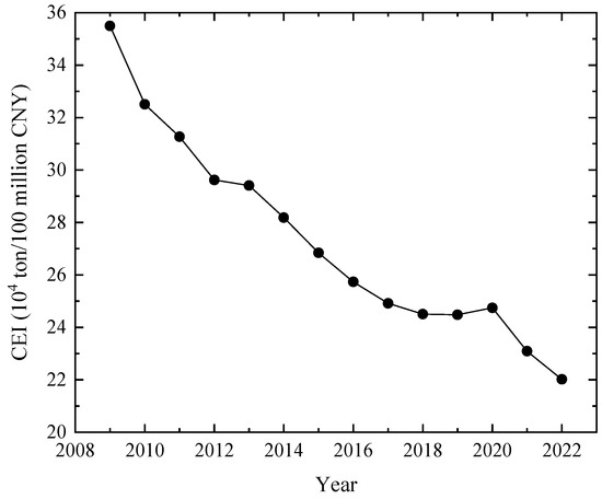
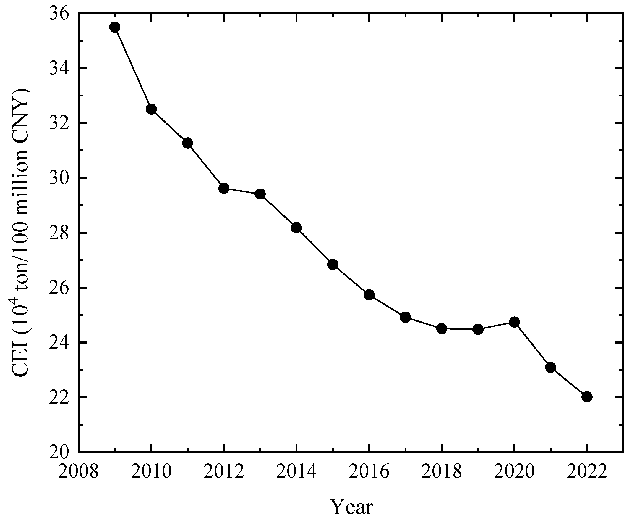
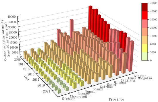
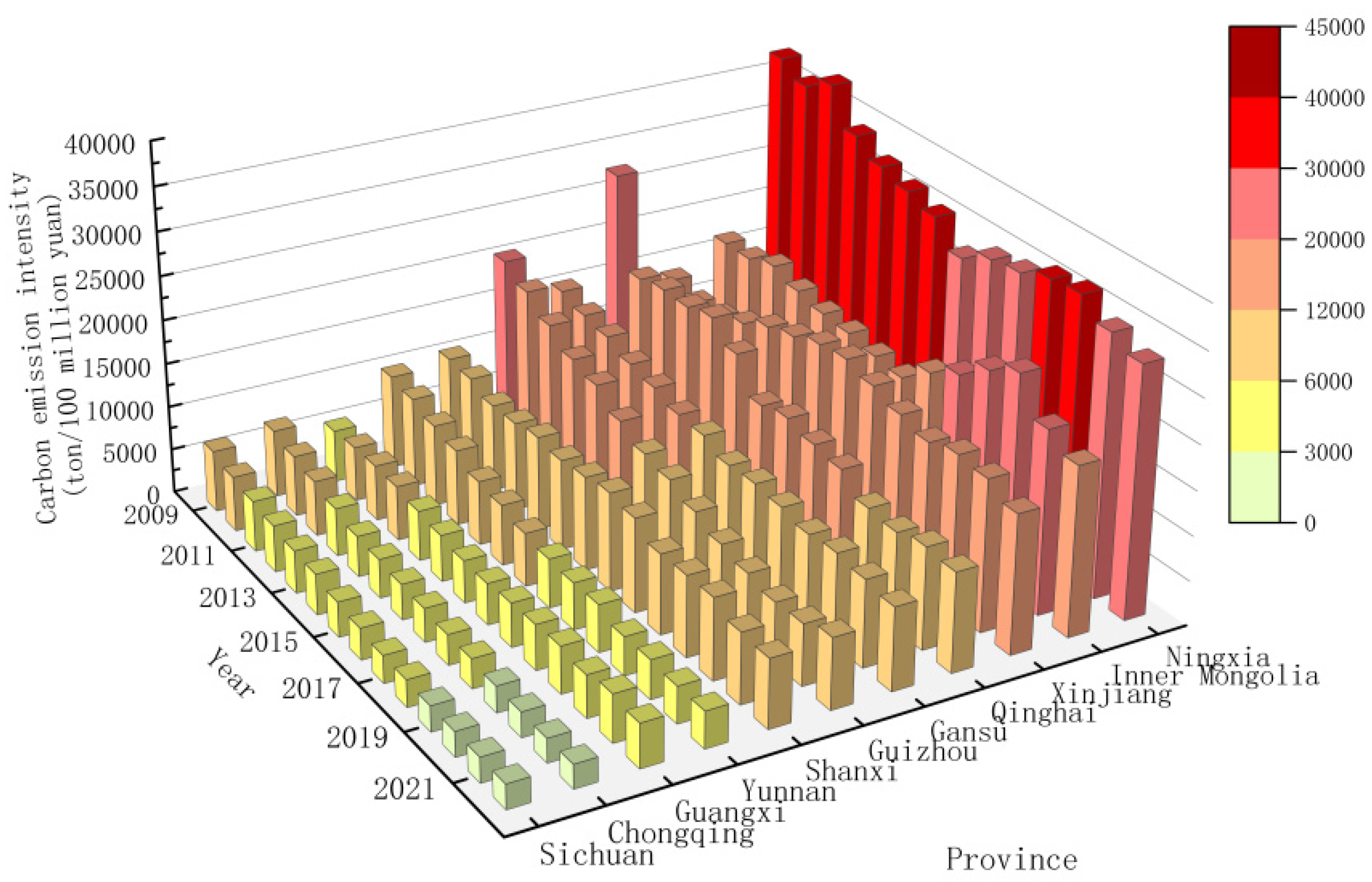
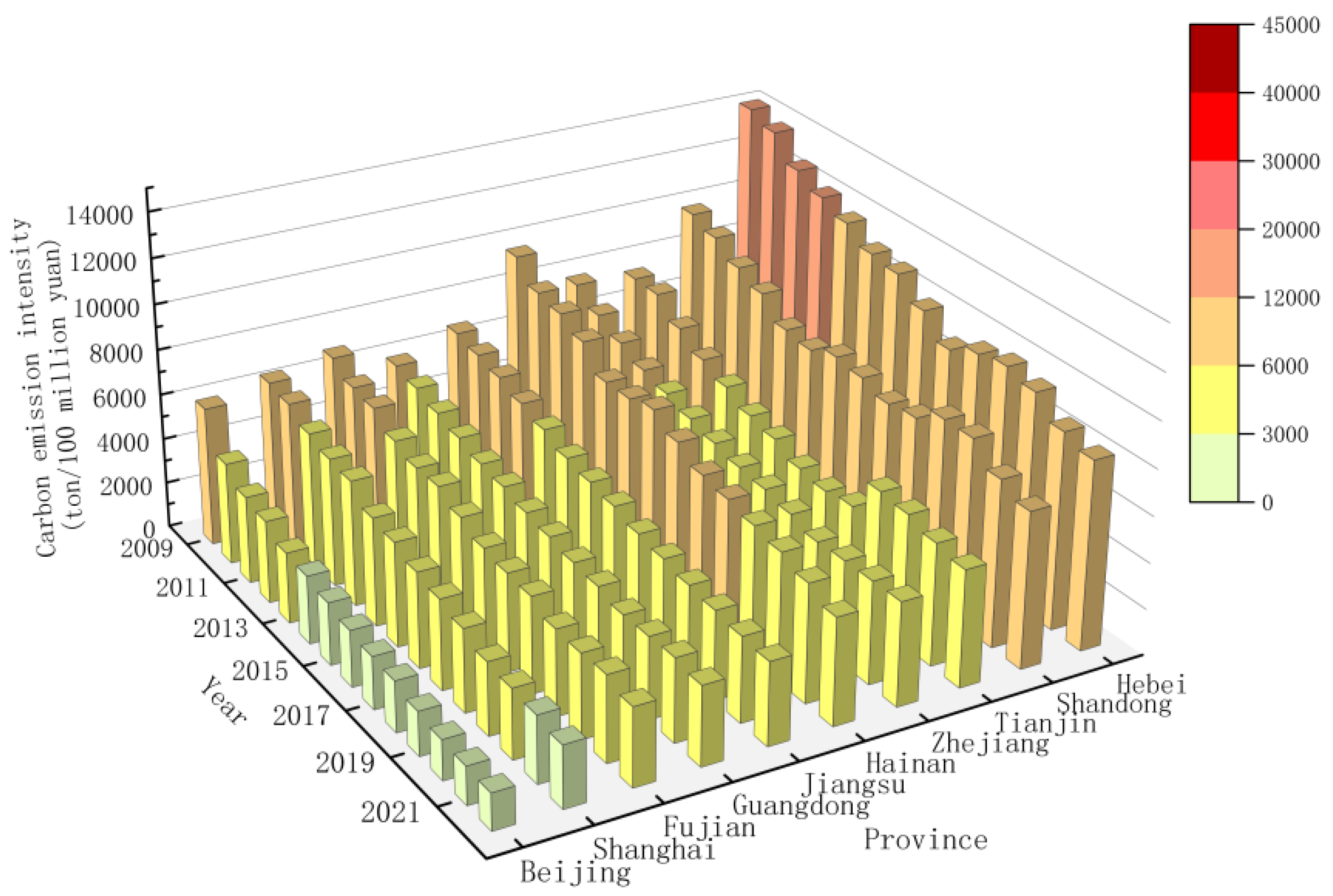
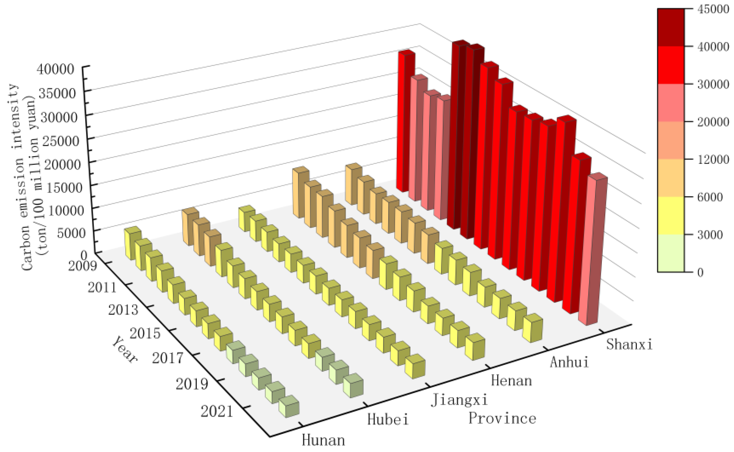
After calculating the CEI of 30 provinces in China from 2009 to 2022, the total CEI of the country is calculated based on Equations (1)–(6). Figure 1 shows China’s CEI from 2009 to 2022. The CEI of western, eastern, central, and northeast regions are shown in Figure 2, Figure 3, Figure 4 and Figure 5.
Figure 1.
CEI of China from 2009 to 2022.
Figure 2.
CEI of western region.
Figure 3.
CEI of eastern region.
Figure 4.
CEI of central region.
Figure 5.
CEI of northeast region.
As shown in Figure 1, China’s CEI exhibited an overall downward trend from 2009 to 2022. By 2022, the CEI had decreased to approximately 60% of that in 2009, while the national GDP in 2022 was about 3.6 times that of 2009. This indicates that over the past 15 years, China’s carbon reduction efforts have been highly effective, with specific carbon reduction targets successfully achieved.
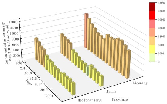
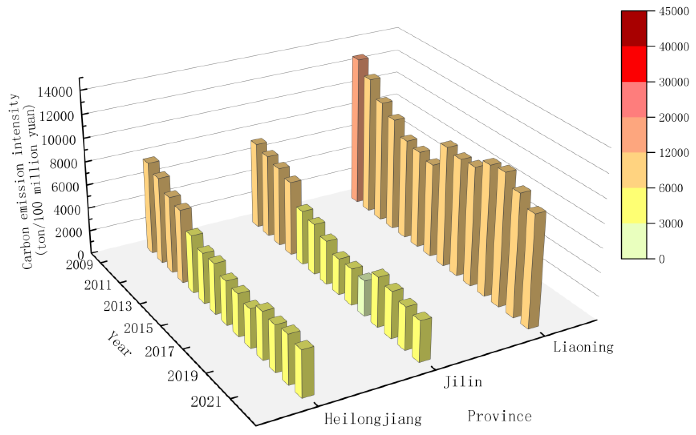
The temporal evolution characteristics of CEI in each province are analyzed. As can be seen from Figure 2, Figure 3, Figure 4 and Figure 5, the CEI of Yunnan, Gansu, Jiangsu, Guangxi, Guizhou, Henan, Jilin, Anhui, Ningxia, Guangdong, Sichuan, Hunan, Hebei, Shandong, Heilongjiang, Hubei, Chongqing, Beijing, Fujian, Jiangxi, Qinghai, Zhejiang, Hainan, and Shanghai showed an overall downward trend. Among them, Shanghai, Beijing, Fujian, Chongqing, Hubei, Guangdong, Sichuan, Hunan, Henan, Jiangsu, Yunnan, and Gansu have the most obvious downward trend of CEI, which is basically a straight-line decline. However, there are also a few provinces whose carbon intensity differs from most. Among them, the CEI of Shanxi Province decreased for a period between 2009 and 2022, but it increased overall, which may be caused by its industrial structure. The proportion of secondary industry in Shanxi Province has always been high, mainly dominated by heavy industry. The CEI of the Inner Mongolia Autonomous Region decreased from 2009 to 2016. Still, it increased significantly from 2016 to 2020, mainly because its energy structure was dominated by coal for a long time, and a large amount of coal production and consumption led to high CEI. The carbon intensity in Liaoning Province increased significantly after 2015 and did not decline until 2020. The CEI in the Xinjiang Autonomous Region rose from 2010 to 2016 and only showed a downward trend after 2016.
4.2.2. Spatial Evolution Characteristics
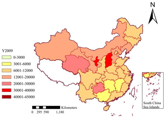
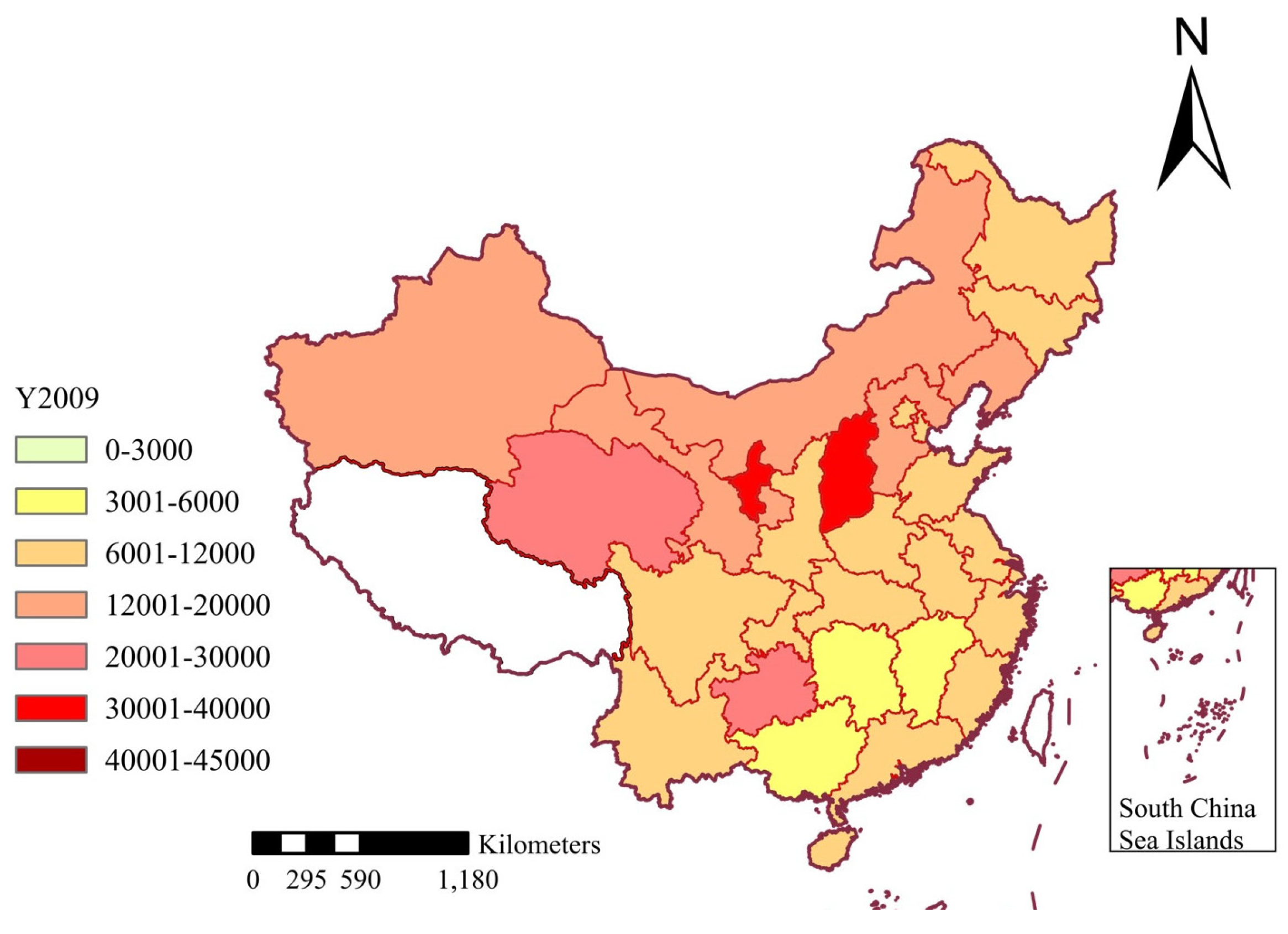
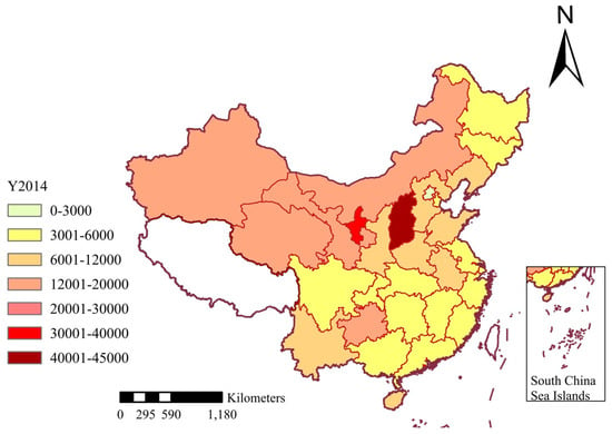
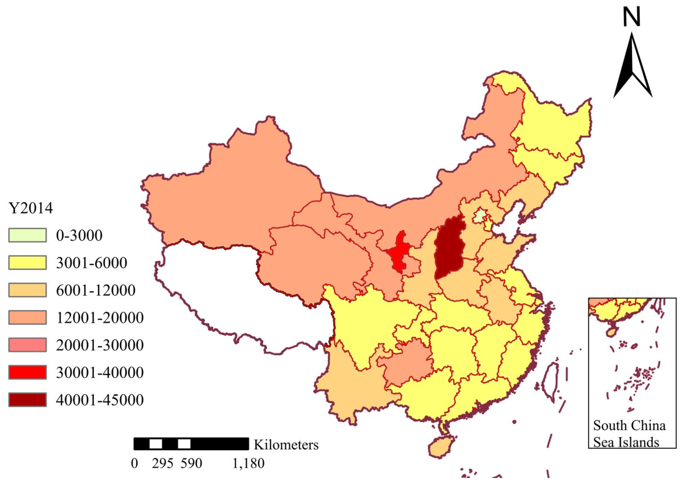
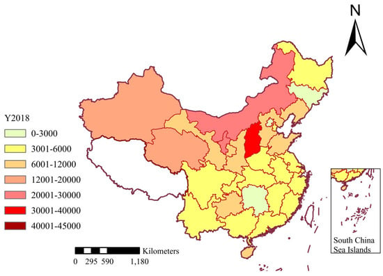
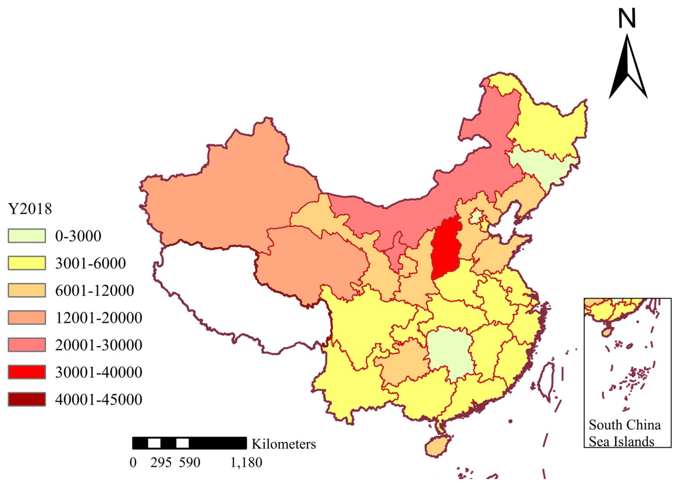
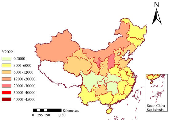
To discuss the differences in CEI between provinces, this study applies ArcGIS to analyze the spatial evolution characteristics. Figure 6, Figure 7, Figure 8 and Figure 9 show the spatial distributions of CEI in 2009, 2014, 2018, and 2022, respectively. In these figures, seven colors are used to rank CEI. Lemongrass color indicates the range from 0 to 3000; autunite yellow indicates the range from 3001 to 6000, which represents a low level of CEI; mango color indicates the range from 6001 to 12,000, which represents a lower level of CEI; cantaloupe color indicates the range from 12,001 to 20,000, which represents a moderate level of CEI; dark coral red indicates the range from 20,001 to 30,000, representing a higher level of CEI; poinsettia red indicates the range from 30,001 to 40,000, representing a high level of CEI; and dark brownish-red indicates the range from 40,001 to 45,000, which represents the highest level of CEI. CEI is measured in tons per billion CYN.
Figure 6.
Spatial distribution of CEI in 2009.
Figure 7.
Spatial distribution of CEI in 2014.
Figure 8.
Spatial distribution of CEI in 2018.
Figure 9.
Spatial distribution of CEI in 2022.
As can be seen from Figure 6, there was no area with a minimum level of CEI in 2009, which shows that no province had a CEI less than 3000 tons per billion CYN, there were only three areas with a low level of CEI at that time, and most provinces’ CEI was concentrated in the range of 6000 tons per billion CYN to 12,000 per billion CYN. From 2009 to 2013, the areas with a low level of CEI gradually increased, and the areas with a lower level of CEI decreased, which intuitively shows that the CEI of the whole country is declining. However, in 2013, for the first time, a region with the highest level of CEI appeared in Shanxi Province, indicating that while the CEI of the country decreased, some provinces also saw an increase in CEI. This may be due to the sudden substantial increase in raw coal consumption in Shanxi Province in 2013 and the lack of an increase in CEI caused by the dramatic increase in regional GDP. In 2014, for the first time, a region with a minimum level of CEI, Beijing, appeared, indicating that the CEI of Beijing was lower than that of the other 29 regions, which is a good signal for the realization of the national carbon reduction plan. After 2015, there are no areas with the highest level of CEI in the country, indicating that Shanxi’s carbon reduction work has been effective, and CEI has been reduced. In 2018, the number of areas with a minimum level of CEI increased to three, and only one area with a high level of CEI remained, reflecting the further success of the country’s carbon reduction efforts. By 2022, there are no areas with a high level of CEI, indicating that areas with a low level of CEI account for the majority. Compared with 2009, it is intuitive to show that the overall CEI of the country has been well controlled, and the effect of carbon reduction work is obvious.
According to China’s four economic regions, the carbon intensity of China’s western region and northeast region showed higher than that of the eastern region and central region in 2009. From Figure 7, by 2014, the overall carbon intensity of western China was higher than that of the other three regions, the overall carbon intensity of northeast China and central China had declined, and the overall carbon intensity of eastern China was the lowest among the four regions. From Figure 8, in 2018, the overall carbon intensity of western China was still higher than that of the other three regions, and there were regions with the lowest carbon intensity in the other three regions. From Figure 9, by 2022, none of China’s four regions will have high carbon emissions.
The results reveal that CEI in China has exhibited a general downward trend since 2009, yet pronounced regional disparities persist. Specifically, southern provinces tend to have lower carbon emission intensities relative to their northern and western counterparts. A more nuanced analysis indicates that this pattern is predominantly shaped by variations in land use types, levels of economic development, and the implementation of policy interventions across different regions.
The main reasons for the decline in carbon emissions are the changes in industrial structure and land use. For instance, northern and western provinces, such as Shanxi and Inner Mongolia, rely heavily on coal mining and heavy industry, which has led to a sustained high level of industrial added value. In Shanxi, the industrial added value has even risen overall, while in Inner Mongolia, it reached its peak during the period from 2016 to 2020. In contrast, the southern and eastern provinces, such as Guangdong and Jiangsu, have shifted towards low-emission industries (services and high-tech), resulting in a greater decline in CEI. For instance, southern provinces such as Guangxi and Yunnan are rich in forests and wetlands, which enhance carbon sequestration to offset emissions and reduce CEI. In the northern regions, where there is a large amount of industrial/mining land and high agricultural emissions (such as fertilizer use), the sink efficiency is relatively weak.
4.3. Spatio-Temporal Correlation Analysis
4.3.1. Spatio-Temporal Agglomeration Analysis
The spatio-temporal correlation of CEI across the 30 regions is obtained via Moran’s I index from Equations (8) and (9). First, the global Moran I index of CEI among these 30 regions is examined. As presented in Table 2, p-value of the global Moran I index shows significant (p < 0.05) in every year. All values of the global Moran’s I index are higher than 0, which means that the global autocorrelation manifests as a positive spatial correlation, reflecting an aggregated pattern across the entire spatial scope.
Table 2.
Results of the global Moran I index.
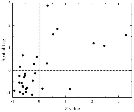
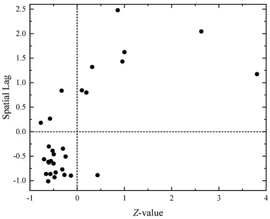
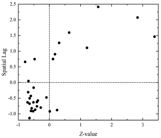
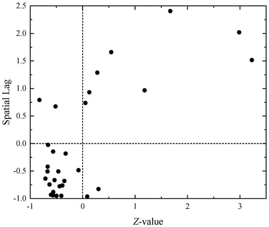
The local Moran I index is computed using Equation (10) to explore the presence of regional spatial aggregation. Based on the calculation results, a Moran scatter plot is generated to illustrate the relationship between the Z-value of spatial deviation and the spatial lag term. The x-axis represents the deviation of the Z-value from its mean: the larger the X-value, the higher CEI level in the region. The y-axis denotes the spatial lag value: the higher the Y-value, the higher CEI level in the surrounding areas.
Figure 10, Figure 11, Figure 12 and Figure 13 present the scatter plots of Moran in 2009, 2014, 2018, and 2022, respectively. The four quadrants are distinguished by the dashed line in these figures, which represent the interrelationships between each region and its neighboring provinces. The first quadrant corresponds to high-high aggregation regions, where both the region itself and its adjacent areas exhibit relatively high CEI, with the spatial association showing a radiative effect. The second quadrant indicates LH aggregation regions, meaning the CEI in the region itself is low.
Figure 10.
Scatter plot of Moran in 2009.
Figure 11.
Scatter plot of Moran in 2014.
Figure 12.
Scatter plot of Moran in 2018.
Figure 13.
Scatter plot of Moran in 2022.
In contrast, the CEI in adjacent regions is high, and the spatial association presents a prominent region of low-value heterogeneity. The third quadrant corresponds to LL aggregation regions, where both the region itself and its adjacent areas have relatively low carbon emission intensities, with the spatial association exhibiting a spatial spillover effect. The fourth quadrant is the HL aggregation region, indicating that the CEI in the region is high while the carbon emission intensities in adjacent regions are low; the spatial association here manifests prominent high-value heterogeneity.
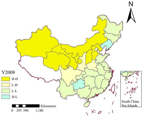
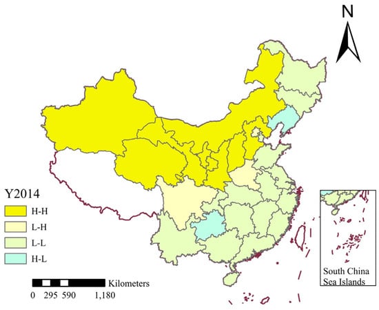
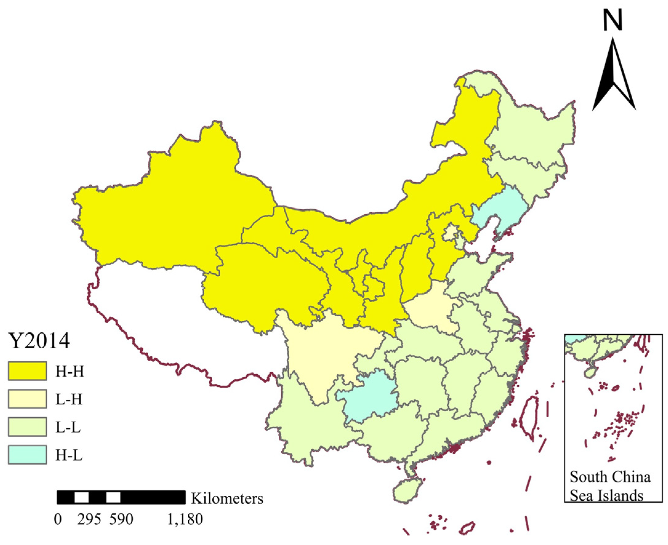
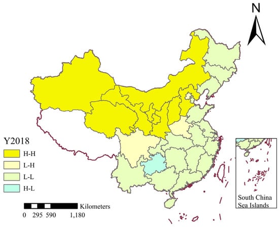
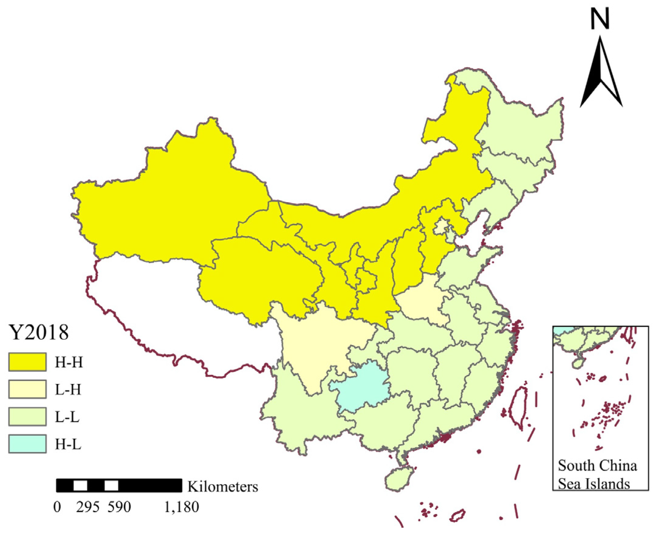
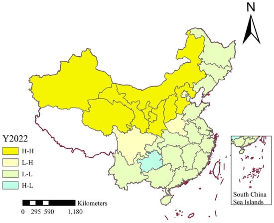
From Figure 10, Figure 11, Figure 12 and Figure 13, over half of the points consistently fall within a single quadrant each year from 2009 to 2022, which means that most provinces have the same spatial clustering effect. It is found that the quadrants of 28 points do not change between 2009 and 2022, which means that the spatial aggregation effect is consistent in 28 provinces during this period. Next, the spatial aggregation effect of 30 provinces is analyzed. Figure 14, Figure 15, Figure 16 and Figure 17 shows the CEI autocorrelation distribution in China in 2009, 2014, 2018, and 2022. First, seven regions have always been in the first quadrant: Hebei, Shanxi, Inner Mongolia, Gansu, Qinghai, Ningxia, and Xinjiang, meaning a HH aggregation of CEI. This indicates that the high CEI of these provinces has a positive impact on the surrounding provinces, driving the increase in CEI of the surrounding provinces. Most of these provinces are located in northern China, and their annual carbon emission consumption is significant. Also, their industrial structure predominantly consists of heavy industries, consequently facing a heightened pressure for low-carbon transformation. Second, Beijing, Henan, and Sichuan have always been in the second quadrant, which means a vulnerability of low-value heterogeneity prominence (LH). This indicates that Beijing, Henan, and Sichuan are independent in terms of carbon intensity, with their local carbon intensity level being lower than that of the surrounding provinces. Third, Anhui, Chongqing, Fujian, Guangdong, Guangxi, Hainan, Heilongjiang, Hubei, Hunan, Jilin, Jiangsu, Jiangxi, Shandong, Shanghai, Tianjin, Yunnan, and Zhejiang are in the third quadrant, which means these provinces are in the LL aggregation. This suggests that the 18 provinces in question exhibit low CEI, as do their neighboring provinces. Furthermore, the development of these provinces has a positive influence on the development of their surrounding regions. Finally, Guizhou is always in the fourth quadrant, indicating there is a high level of CEI in Guizhou and a low level in its neighboring areas. Therefore, Guizhou needs to develop cooperatively with neighboring provinces and strive to reduce CEI to the same level as neighboring provinces as soon as possible.
Figure 14.
CEI autocorrelation distribution in 2009.
Figure 15.
CEI autocorrelation distribution in 2014.
Figure 16.
CEI autocorrelation distribution in 2018.
Figure 17.
CEI autocorrelation distribution in 2022.
By contrast, the CEI in adjacent regions is high, and the spatial association presents a prominent area of low-value heterogeneity. The third quadrant represents LL aggregation regions, where both the region itself and its adjacent areas have relatively low carbon emission intensities, with the spatial association exhibiting a spatial spillover effect. The fourth quadrant corresponds to HL aggregation regions, indicating that the region has a high CEI while its adjacent regions have low carbon emission intensities; the spatial association here is characterized by prominent high-value heterogeneity.
Most of the provinces in the HH cluster are located in the northern and northwestern regions, such as coal in Shanxi and Inner Mongolia, and oil and gas in Xinjiang, and are the core energy strategic bases of the country. Their socio-economic structure is highly dependent on the mining, processing, and export of energy and raw materials. Therefore, their industrial systems are generally dominated by high-energy-consuming and high-carbon-emitting heavy industries such as coal, thermal power, metallurgy, chemical engineering, and building materials, forming a single industrial path dependence. LL clusters are concentrated in the eastern coastal areas and some central provinces, such as Jiangsu, Zhejiang, Guangdong, Shanghai, etc. These regions have superior socio-economic conditions, and their economic growth comes more from technological innovation, high-end manufacturing, and modern service industries, rather than energy intensive industries. At the same time, as the forefront of reform and opening up, they usually have more advanced production technology, stricter environmental regulations, and more comprehensive green financial support, resulting in significantly higher energy utilization efficiency. In addition, the close economic connections and industrial cooperation within urban agglomerations such as the Yangtze River Delta and the Pearl River Delta have resulted in a synergistic effect of low-carbon development models throughout the region.
The results of local CEI agglomeration across the 30 provinces indicate that spatial agglomeration is primarily concentrated in HH and LL agglomeration areas. From a geographical distribution perspective, HH spatial agglomeration is mainly observed in China’s central and western regions, where the high CEI exerts a negative spatial spillover effect on neighboring provinces. It leads to relatively high CEI levels in adjacent areas. In contrast, most LL regions are clustered in China’s eastern and southern regions; the lower CEI levels here generate a positive spatial spillover effect on neighboring provinces, driving progress in carbon reduction efforts in adjacent areas. Overall, the majority of China’s provinces fall within the third quadrant, suggesting that China’s overall CEI level is developing favorably. This trend holds significant importance for the country in achieving the ‘Dual Carbon’ goals.
4.3.2. Spatio-Temporal Leap Analysis
Regarding spatio-temporal transition, 28 provinces remained stable during 2009–2022, but Liaoning and Shaanxi Provinces showed characteristics of spatio-temporal transition, revealing the spatio-temporal evolution pattern of their CEI.
Liaoning Province, positioned in the fourth quadrant from 2009 to 2014 and the third quadrant from 2015 to 2022, demonstrated a high CEI during the earlier period, contrasting with the lower intensity of its neighboring provinces. It suggests that Liaoning Province exerted a negative spatial spillover effect on the CEI levels of adjacent provinces from 2009 to 2014.
Shaanxi Province, located in the second quadrant in 2009 and the first quadrant from 2010 to 2022, shows that in 2009, it had a lower CEI than its surrounding regions. However, from 2010 onwards, Shaanxi Province’s CEI has increased, surpassing that of its neighboring areas.
The observed spatio-temporal patterns and regional disparities provide insights into the underlying drivers of CEI and have important implications for carbon reduction policies in China. The underlying drivers of CEI are variations in land use types, economic development level, and the implementation of policy interventions. Specifically, southern provinces, such as Guangxi and Yunnan, have extensive forest land and wetlands acting as strong natural carbon sinks through photosynthesis and soil carbon storage (Section 3.2.4), while northern and western regions have more industrial/mining construction land and cultivated land with higher agricultural emissions (e.g., from fertilizer use and machinery energy consumption), leading to higher net emissions relative to their carbon sink capacity. Eastern and southern provinces, such as Guangdong and Jiangsu, have shifted from energy-intensive industries to high-tech and service sectors generating higher GDP with lower emissions, reducing CEI through higher economic output per unit energy, whereas northern and western provinces remain reliant on coal mining and heavy industries, tying economic growth to high energy consumption and resulting in persistently high CEI. The provinces with stricter, earlier low-carbon policies, such as Beijing and Shanghai, achieved steeper CEI declines by phasing out high-emission industries and investing in renewable energy, while western provinces, despite national support (e.g., Western Development Strategy), face slower technological upgrading and limited financial resources that slow their CEI reduction progress.
4.4. Discussion
The findings that land use change significantly impacts carbon emissions support previous research [7,8,9]. China’s CEI is generally on a downward trend, but there are significant regional differences. Particularly, the CEI in southern and eastern provinces has decreased significantly and at a faster rate. In contrast, northern and western provinces have shown persistently high CEI. Spatially, this difference is manifested as a ‘low in the south and high in the north’ pattern. The LL clusters are concentrated in the southern and eastern regions, while the HH clusters are concentrated in the northern and western industrial and resource-rich regions. These results are roughly the same as those in the existing literature [45,46,47]. Ref. [21] found that carbon emissions have spatial spillover effects and regional heterogeneity, which is consistent with the findings of China’s CEI pattern in this study. The clustering of HH and LL is obvious, which is in accordance with the conclusions of ref. [21], and further strengthens the findings of regional economic structure driving carbon emissions in Refs. [15,23] through provincial cases such as Shaanxi and Liaoning.
Regarding the relationship between economic development and LUCEs, multiple studies [15,16,17] have pointed out that GDP growth directly drives up carbon emissions, especially through the expansion of construction land and industrial activities. It is found that CEI shows a trend of decreasing first and then increasing, indirectly confirming the positive correlation between economic expansion and carbon emissions, which is consistent with ref. [15] on the dominant role of GDP. The relationship between economic development and LUCEs obtained in this study corresponds to the nonlinear law of increasing carbon emissions first and then reducing emissions in ref. [20].
4.5. Limitations and Future Research
There are some limitations. Firstly, regarding data scale, the provincial-level CEI analysis may mask significant spatial heterogeneity within provinces, as land use carbon emission patterns could vary substantially across different prefecture-level cities within the same province. Secondly, the carbon emission factor method may fail to accurately reflect regional specificity due to inter-provincial differences in energy structures, and it cannot fully capture indirect carbon emissions from land use changes. Finally, while the study proposes land use planning recommendations, it lacks quantitative predictions of policy effects under different scenarios.
Future research can use municipal and county-level data, or combine auxiliary information such as nighttime light data, to improve spatial accuracy. More transparent and standardized reporting protocols for provincial statistics are needed. Process-based models (e.g., CLUE-S) with life-cycle assessment methods can be integrated to improve emission accounting precision. Subsequently, a spatial explicit optimization model can be developed to simulate the implementation effects of various planning schemes.
5. Conclusions
This paper aims to investigate the spatio-temporal evolution and differences in CEI across different land use types in China from perspectives of time and space. In conclusion, this study found that CEI in China has declined overall but with significant regional disparities. The observed spatio-temporal patterns and regional disparities provide important insights into the underlying drivers of CEI and have implications for carbon reduction policies. This study proposes the following conclusions.
- (1)
- Even though China’s overall CEI has shown a downward trend since 2009, local CEI still fluctuates and even has an upward trend. The CEI had decreased to approximately 60% of that in 2009, while the national GDP in 2022 was about 3.6 times that of 2009. Moreover, China’s CEI varies greatly among regions, with the CEI of southern provinces being significantly lower than that of northern provinces and eastern provinces being considerably lower than that of western provinces.
- (2)
- The LUCEs and economic development in China’s 30 provinces exhibited weak decoupling in most years. In 2020, however, their relationship shifted to expanding correlation.
- (3)
- The spatial aggregation effect of CEI in 30 provinces in China is noticeable, and most of them are clustered in HH or LL regions, indicating that the spatial differences in CEI in China still exist. Provinces such as Liaoning and Shaanxi exhibit spatio-temporal transition characteristics.
Policymakers should consider regional differences in CEI when formulating carbon reduction targets and strategies. Additionally, promoting sustainable land use practices and low-carbon technologies can help lower carbon emissions and alleviate the effects of climate change [48]. The government can formulate policies and take actions in three aspects: industrial structure adjustment, regional coordination, and land planning.
Firstly, to advance industrial restructuring, HH regions should strictly eliminate outdated production capacity, promote hydrogen steelmaking and carbon capture technologies, and build integrated wind solar hydrogen storage bases based on the natural resources of these regions. LL regions can develop strategic emerging industries to cultivate low-carbon industrial clusters, such as digital economy and green finance, implementing supply chain carbon neutrality [49].
Secondly, for regional coordination, the government can establish regional cooperation mechanisms to facilitate cooperation and exchanges between provinces with different carbon emission intensities. A carbon transfer payment system can be established to encourage LL regions to help HH ones reduce carbon emissions through technology transfer and financial support. Enterprises in LL regions can be encouraged to export low-carbon technologies to HH regions, forming a positive spillover effect.
Thirdly, in terms of land planning, HH regions should strictly control the expansion of construction land and promote the industrial–ecological composite land use model. The linkage mechanism between construction land indicators and the redevelopment of existing inefficient land can be promoted to improve intensive utilization. LL regions can develop compact cities and fully tap into the carbon sequestration potential of forests and wetlands. Urban spatial layout can be optimized to develop green infrastructure [50].
Author Contributions
Conceptualization, J.C.; methodology, C.C. (Changhong Cai); software, C.C. (Changhong Cai); validation, C.C. (Changqing Chen); formal analysis, J.C.; investigation, M.Z.; data curation, J.G.; writing—original draft preparation, J.C.; writing—review and editing, M.Z.; visualization, J.C. and J.G.; supervision, Y.L.; project administration, X.C.; funding acquisition, J.C. All authors have read and agreed to the published version of the manuscript.
Funding
This research was funded by National Natural Science Foundation of China (Grant No. 62306182) and Guangdong Basic and Applied Basic Research Foundation (Grant No. 2022A1515110378).
Data Availability Statement
The data presented in this study are available on request from the corresponding author (Some data is subject to copyright restrictions due to collection channels).
Conflicts of Interest
Author Jun Guan and Changqing Chen were employed by China State Civil Engineering Limited and China State Construction International Holdings Limited. The remaining authors declare that the research was conducted in the absence of any commercial or financial relationships that could be construed as a potential conflict of interest.
Abbreviations
The following abbreviations are used in this manuscript:
| IPCC | Intergovernmental Panel on Climate Change |
| GDP | Gross domestic product |
| HH | High-high |
| LL | Low-low |
| CEI | Carbon emission intensity |
| LUCEs | Land use carbon emissions |
| SD | Strong decoupling |
| WD | Weak decoupling |
| EC | Expansion connection |
Appendix A
Table A1.
Sources of carbon emission and carbon emission coefficient of cultivated land.
Table A2.
Carbon emission coefficients and standard coal coefficients of the energy sources.
Table A3.
Water content, carbon absorption rate, and economic coefficient of agricultural crop.
Table A4.
Carbon emission coefficient of various land use types.
References
- Intergovernmental Panel on Climate Change (IPCC). Climate Change 2013: The Physical Science Basis. Contribution of Working Group I to the Fifth Assessment Report of the Intergovernmental Panel on Climate Change; Cambridge University Press: Cambridge, UK, 2013. [Google Scholar]
- UN-Habitat. World Cities Report 2020; United Nations Human Settlements Programme (UN-Habitat); UN-Habitat: Nairobi, Kenya, 2020. [Google Scholar]
- Rong, T.; Zhang, P.; Zhu, H.; Jiang, L.; Li, Y.; Liu, Z. Spatial correlation evolution and prediction scenario of land use carbon emissions in China. Ecol. Inform. 2022, 71, 101802. [Google Scholar] [CrossRef] [Scilit]
- Song, C.; Zhao, T.; Wang, J. Spatial-temporal analysis of China’s regional carbon intensity based on ST-IDA from 2000 to 2015. J. Clean. Prod. 2019, 238, 117874. [Google Scholar] [CrossRef] [Scilit]
- Dietz, T.; Gardner, G.T.; Gilligan, J.; Stern, P.C.; Vandenbergh, M.P. Household actions can provide a behavioral wedge to rapidly reduce US carbon emissions. Proc. Natl. Acad. Sci. USA 2009, 106, 18452–18456. [Google Scholar] [CrossRef] [Scilit] [PubMed]
- Zhang, W.; Lin, H.; Zhu, Q.; Gan, H.; Ren, Y.; Yang, Z. Evolution trend analysis of carbon emissions in light industrial parks: A system dynamics approach. Energy Sci. Eng. 2023, 11, 3721–3737. [Google Scholar] [CrossRef] [Scilit]
- Li, H.; Mu, H.; Zhan, M.; Li, N. Analysis on influence factors of China’s CO2 emissions based on Path–STIRPAT model. Energy Policy 2011, 39, 6906–6911. [Google Scholar] [CrossRef] [Scilit]
- Shen, G.; Yang, Y.; Wang, W.; Tao, S.; Zhu, C.; Min, Y.; Xue, M.; Ding, J.; Wang, B.; Wang, R.; et al. Emission factors of particulate matter and elemental carbon for crop residues and coals burned in typical household stoves in China. Environ. Sci. Technol. 2010, 44, 7157–7162. [Google Scholar] [CrossRef] [Scilit]
- Simmonds, M.B.; Di Vittorio, A.V.; Jahns, C.; Johnston, E.; Jones, A.; Nico, P.S. Impacts of California’s climate-relevant land use policy scenarios on terrestrial carbon emissions (CO2 and CH4) and wildfire risk. Environ. Res. Lett. 2021, 16, 014044. [Google Scholar] [CrossRef] [Scilit]
- Wang, F.; Sun, X.; Reiner, D.M.; Wu, M. Changing trends of the elasticity of China’s carbon emission intensity to industry structure and energy efficiency. Energy Econ. 2020, 86, 104679. [Google Scholar] [CrossRef] [Scilit]
- Li, Y. A review on carbon emission accounting approaches for the electricity power industry. Appl. Energy 2024, 359, 122681. [Google Scholar] [CrossRef] [Scilit]
- La Notte, A.; Tonin, S.; Lucaroni, G. Assessing direct and indirect emissions of greenhouse gases in road transportation, taking into account the role of uncertainty in the emissions inventory. Environ. Impact Assess. Rev. 2018, 69, 82–93. [Google Scholar] [CrossRef] [Scilit]
- Wu, M.; Shi, J.; Wen, H.; Qiu, Y.; Guo, C. Research on power and energy balance of new power system under low carbon emission path. Energy Rep. 2022, 8, 197–207. [Google Scholar] [CrossRef] [Scilit]
- Wei, W.; Li, Y.; Ma, L.; Xie, B.; Hao, R.; Chen, D.; Yang, S. Carbon emission change based on land use in Gansu Province. Environ. Monit. Assess. 2024, 196, 311. [Google Scholar] [CrossRef] [Scilit]
- Fang, W.; Luo, P.P.; Luo, L.T.; Zha, X.B.; Nover, D. Spatio-temporal characteristics and influencing factors of carbon emissions from land-use change in Shaanxi Province, China. Environ. Sci. Pollut. Res. 2023, 30, 123480–123496. [Google Scholar] [CrossRef] [Scilit]
- Liu, C.; Hu, S.G.; Wu, S.; Song, J.R.; Li, H.Y. County-level land use carbon emissions in China: Spatio-temporal patterns and impact factors. Sustain. Cities Soc. 2024, 105, 105304. [Google Scholar] [CrossRef] [Scilit]
- He, Q.; Yuan, Q.; Chen, X.; Jiang, P.; Wang, Y.; Li, Y. Research on industry–economy–energy–carbon emission relationships based on panel vector autoregressive modeling. Processes 2025, 13, 1107. [Google Scholar] [CrossRef] [Scilit]
- Zhu, Q.; Peng, X. The impacts of population change on carbon emissions in China during 1978–2008. Environ. Impact Assess. Rev. 2012, 36, 1–8. [Google Scholar] [CrossRef] [Scilit]
- Liu, R.; Fang, Y.R.; Peng, S.; Benani, N.; Wu, X.; Chen, Y.; Wang, T.; Chai, Q.; Yang, P. Study on factors influencing carbon dioxide emissions and carbon peak heterogenous pathways in Chinese provinces. J. Environ. Manag. 2024, 365, 121667. [Google Scholar] [CrossRef] [Scilit]
- Cui, H.; Zhao, T.; Shi, H. STIRPAT-based driving factor decomposition analysis of agricultural carbon emissions in Hebei, China. Pol. J. Environ. Stud. 2018, 27, 1449–1461. [Google Scholar] [CrossRef] [Scilit]
- Wang, H.H.; He, Y.Y.; Shi, W.Y.; Zeng, W.H.; He, Y.F. Spatio-temporal spillover effect and efficiency of carbon emissions from land use in China. Environ. Dev. Sustain. 2024, 26, 8915–8953. [Google Scholar] [CrossRef] [Scilit]
- Wu, S.; Hu, S.G.; Frazier, A.E. Spatio-temporal variation and driving factors of carbon emissions in three industrial land spaces in China from 1997 to 2016. Technol. Forecast. Soc. Change 2021, 169, 120837. [Google Scholar] [CrossRef] [Scilit]
- Dai, F.; Zhan, M.; Chen, X.; Yang, X.; Ouyang, P. Spatio-temporal evolution and driving factors of land use carbon emissions in Jiangxi Province, China. Forests 2024, 15, 1825. [Google Scholar] [CrossRef] [Scilit]
- Clarke-Sather, A.; Qu, J.S.; Wang, Q.; Zeng, J.J.; Li, Y. Carbon inequality at the sub-national scale: A case study of provincial-level inequality in CO2 emissions in China 1997–2007. Energy Policy 2011, 39, 5420–5428. [Google Scholar] [CrossRef] [Scilit]
- Zhang, Y.J.; Hao, J.F.; Song, J. The CO2 emission efficiency, reduction potential and spatial clustering in China’s industry: Evidence from the regional level. Appl. Energy 2016, 174, 213–223. [Google Scholar] [CrossRef] [Scilit]
- Fan, F.; Dai, S.; Yang, B.; Ke, H. Urban density, directed technological change, and carbon intensity: An empirical study based on Chinese cities. Technol. Soc. 2023, 72, 102151. [Google Scholar] [CrossRef] [Scilit]
- Fan, M.J.; Wang, Z.Q.; Xue, Z.B. Spatio-temporal evolution characteristics, influencing factors of land use carbon emissions, and low-carbon development in Hubei Province, China. Ecol. Inform. 2024, 81, 102567. [Google Scholar] [CrossRef] [Scilit]
- Zhu, E.Y.; Li, W.; Chen, L.S.; Sha, M. Spatio-temporal coupling analysis of land urbanization and carbon emissions: A case study of Zhejiang Province, China. Land Degrad. Dev. 2023, 34, 4594–4606. [Google Scholar] [CrossRef] [Scilit]
- Cheng, Y.X.; Tang, Y.Q.; Zhou, B.; Feng, H.H. Spatio-temporal analysis of national carbon emission and regional carbon simulation in China. Environ. Sci. Pollut. Res. 2024, 31, 10702–10716. [Google Scholar] [CrossRef] [Scilit]
- Yang, S.J.; Wen, L.J.; Zhang, A.L. The spatio-temporal response of land-use carbon emissions to climate change. Ecol. Indic. 2025, 170, 112893. [Google Scholar] [CrossRef] [Scilit]
- Zhang, T.; Chen, L.; Yu, Z.; Zang, J.; Li, L. Spatio-temporal evolution characteristics of carbon emissions from industrial land in Anhui Province, China. Land 2022, 11, 2084. [Google Scholar] [CrossRef] [Scilit]
- Li, L.; Huang, X.; Yang, H. Optimizing land use patterns to improve the contribution of land use planning to carbon neutrality target. Land Use Policy 2023, 135, 106959. [Google Scholar] [CrossRef] [Scilit]
- Chuai, X.; Huang, X.; Yang, H.; Zhang, M.; Zhong, T.; Zhang, M.; Chen, Z.; Chen, Y.; Wang, X.; Thompson, J.R. Land use, total carbon emissions change and low carbon land management in Coastal Jiangsu, China. J. Clean. Prod. 2015, 103, 77–86. [Google Scholar] [CrossRef] [Scilit]
- Tian, M.; Chen, Z.; Wang, W.; Chen, T.; Cui, H. Land-use carbon emissions in the Yellow River Basin from 2000 to 2020: Spatio-temporal patterns and driving mechanisms. Int. J. Environ. Res. Public Health 2022, 19, 16507. [Google Scholar] [CrossRef] [Scilit] [PubMed]
- Yu, Y.; Du, C.; Xu, X.; Hu, C.; Zeng, J.; Li, E.; Miao, H.; Liu, K. Research on land use carbon emissions empirical in Guangdong Province. In Resources and Sustainable Development; Wu, J., Lu, X., Xu, H., Nakagoshi, N., Eds.; Trans Tech Publications Ltd.: Zurich, Switzerland, 2013; Pts 1–4, Volumes 734–737, p. 1929. [Google Scholar]
- Wang, G.; Liao, M.; Jiang, J. Research on agricultural carbon emissions and regional carbon emissions reduction strategies in China. Sustainability 2020, 12, 2627. [Google Scholar] [CrossRef] [Scilit]
- Hua, J.; Gao, J.; Chen, K.; Li, J. Driving effect of decoupling provincial industrial economic growth and industrial carbon emissions in China. Int. J. Environ. Res. Public Health 2023, 20, 145. [Google Scholar] [CrossRef] [Scilit]
- Zhou, H.; Cao, J. The decoupling of carbon emissions from economic growth in Jiangsu, China: 2000–2010. In LTLGB 2012: Proceedings of the International Conference on Low-Carbon Transportation and Logistics, and Green Buildings, Beijing, China, 2–13 October 2012; Chen, F., Liu, Y., Hua, G., Eds.; Springer: Berlin, Germany, 2012; Volume 1, pp. 937–943. [Google Scholar]
- Maier, M.; Mueller, M.; Yan, X. Introducing a localised spatio-temporal LCI method with wheat production as exploratory case study. J. Clean. Prod. 2017, 140, 492–501. [Google Scholar] [CrossRef] [Scilit]
- Wang, J.F.; Zhang, T.L.; Fu, B.J. A measure of spatial stratified heterogeneity. Ecol. Indic. 2016, 67, 250–256. [Google Scholar] [CrossRef] [Scilit]
- Tiefelsdorf, M.; Boots, B. The exact distribution of Moran, I. Environ. Plan. A 1995, 27, 985–999. [Google Scholar] [CrossRef] [Scilit]
- LeSage, J.P.; Pace, R.K. Introduction to Spatial Econometrics; CRC Press: Boca Raton, FL, USA, 2009. [Google Scholar]
- Anselin, L.; Cliff, A.D.; Ord, J.K. Spatial processes, models and applications. Econ. Geogr. 1983, 59, 322. [Google Scholar] [CrossRef] [Scilit]
- Anselin, L. Local Indicators of Spatial Association—LISA. Geogr. Anal. 1995, 27, 93–115. [Google Scholar] [CrossRef] [Scilit]
- Cai, B.F.; Wang, X.Q.; Huang, G.H.; Wang, J.N.; Cao, D.; Baetz, B.W.; Liu, L.; Zhang, H.; Fenech, A.; Liu, Z. Spatiotemporal changes of China’s carbon emissions. Geophys. Res. Lett. 2018, 45, 8536–8546. [Google Scholar] [CrossRef] [Scilit]
- Wu, H.; Yang, Y.; Shen, Y. Agricultural carbon emissions in China: Estimation, influencing factors, and projection of peak emissions. Pol. J. Environ. Stud. 2024, 33, 4791–4806. [Google Scholar] [CrossRef] [Scilit]
- Tian, G.; Yu, S.; Wu, Z.; Xia, Q. Study on the emission reduction effect and spatial difference of carbon emission trading policy in China. Energies 2022, 15, 1921. [Google Scholar] [CrossRef] [Scilit]
- Cheng, J.; Xie, Y.; Zhang, J. Industry structure optimization via the complex network of industry space: A case study of Jiangxi Province in China. J. Clean. Prod. 2022, 338, 130602. [Google Scholar] [CrossRef] [Scilit]
- Cheng, J.; Cai, C.H. The optimization of industrial structure under the ‘Dual Carbon’ Goal via multi-objective programming model: Evidence from Guangdong Province, China. Sustainability 2025, 17, 5912. [Google Scholar] [CrossRef] [Scilit]
- Ghosh, S.; Dinda, S.; Das Chatterjee, N.; Dutta, S.; Bera, D. Spatial-explicit carbon emission-sequestration balance estimation and evaluation of emission susceptible zones in an Eastern Himalayan city using Pressure-Sensitivity-Resilience framework: An approach towards achieving low carbon cities. J. Clean. Prod. 2022, 336, 130417. [Google Scholar] [CrossRef] [Scilit]

Disclaimer/Publisher’s Note: The statements, opinions and data contained in all publications are solely those of the individual author(s) and contributor(s) and not of MDPI and/or the editor(s). MDPI and/or the editor(s) disclaim responsibility for any injury to people or property resulting from any ideas, methods, instructions or products referred to in the content. |
© 2025 by the authors. Licensee MDPI, Basel, Switzerland. This article is an open access article distributed under the terms and conditions of the Creative Commons Attribution (CC BY) license (https://creativecommons.org/licenses/by/4.0/).