Article

Research on Risk Evolution Probability of Urban Lifeline Natech Events Based on MdC-MCMC

School of Management, China University of Mining and Technology (Beijing), Beijing 100083, China
*
Author to whom correspondence should be addressed.
Sustainability 2025, 17(17), 7664; https://doi.org/10.3390/su17177664
Submission received: 23 June 2025 / Revised: 21 August 2025 / Accepted: 22 August 2025 / Published: 25 August 2025

Abstract

Urban lifeline Natech events are coupled systems composed of multiple risks and entities with complex dynamic transmission chains. Predicting risk evolution probabilities is the core task for achieving the safety management of urban lifeline Natech events. First, the risk evolution mechanism is analyzed, where urban lifeline Natech events exhibit spatial evolution characteristics, which involves dissecting the parallel and synergistic effects of risk evolution in spatial dimensions. Next, based on fitting marginal probability distribution functions for natural hazard and urban lifeline risk evolution, a Multi-dimensional Copula (MdC) function for the joint probability distribution of urban lifeline Natech event risk evolution is constructed. Building upon the MdC function, a Markov Chain Monte Carlo (MCMC) model for predicting risk evolution probabilities of urban lifeline Natech events is developed using the Metropolis–Hastings (M-H) algorithm and Gibbs sampling. Finally, taking the 2021 Zhengzhou ‘7·20’ catastrophic rainstorm as a case study, joint probability distribution functions for risk evolution under Rainfall-Wind speed scenarios are fitted for traffic, electric, communication, water supply, and drainage systems (including different risk transmission chains). Numerical simulations of joint probability distributions for risk evolution are conducted, and visualizations of joint probability predictions for risk evolution are generated.

1. Introduction

The safety of urban lifelines directly affects the high-quality development of cities and the well-being of residents, while the occurrence and evolution of natural hazards have posed a severe threat to urban lifeline safety. In recent years, numerous scholars have continuously explored the field of natural hazards and urban lifeline safety, specifically researching Natech (Natural hazard-triggered technological accident) events in urban lifelines. Among these, predicting the probability of risk evolution serves as a forward-looking guide and decision-making support for the risk management of urban lifeline Natech events.
Natural hazards may lead to catastrophic technical accidents in the urban lifeline. For example, flood disasters can trigger catastrophic failures in interdependent urban traffic networks. Yadav et al. [1] constructed a hypothesis-driven resilience framework to analyze the impact of flood disasters on urban traffic networks. Chen et al. [2] established a Bayesian network-based risk assessment and sensitivity analysis framework, analyzing power tunnel risk accident cases. Based on the operational data of Beijing Future Science and Technology City from 2010 to 2018, the K 2 algorithm was used to obtain the conditional probabilities of nodes in the Bayesian networks, describing and demonstrating the groundwater accident evolution process in power tunnels, identifying and predicting critical points and risk probabilities of accidents. In terms of urban drainage systems, Henonin et al. [3] developed an alluvial flood model for urban areas, classifying urban flood systems to address the prediction of comprehensive urban flood risk management. Fu et al. [4] fitted rainfall data and applied a Monte Carlo simulation for uncertainty propagation to calculate the exceedance probability of flood volumes in urban drainage systems. Koukoui et al. [5] adopted the “Adaptive Critical Point-Opportunity” method to predict critical points of natural hazards such as floods, droughts, and heatwaves, aiming to resolve safety management challenges in drainage systems and other urban lifelines. Piadeh et al. [6] proposed a dynamic ensemble data mining model to predict the relationship between urban drainage systems and flood disasters, providing support for implementing risk management actions. Zheng et al. [7] employed a data-driven approach, utilizing flood disaster and drainage system monitoring data to achieve forecasting and the prediction of urban waterlogging. Coastal cities often face typhoons and urban waterlogging, resulting in power outages and significant economic losses. Ma et al. [8] proposed a method to predict grid failure rates during typhoons and waterlogging, suggesting strategies to enhance grid resilience after disasters. Bagheri et al. [9] and Wang et al. [10] calculated the failure probability of transmission chains under typhoon disasters, identifying vulnerable lines in transmission systems under such scenarios. Urban heating systems face substantial threats from earthquakes and other natural hazards. Mao et al. [11] adopted a comprehensive fault probability method to directly calculate the comprehensive failure probability of heating pipelines in known seismic zones.
Through summarizing the aforementioned research findings, it is observed that studies on the risk evolution of Natech events in urban lifelines have predominantly focused on predicting the probability of risk evolution for individual urban lifelines under single or simply compounded natural disasters. However, the urban lifeline Natech event is actually a system with complex dynamic risk transmission chains [12]. In the spatial dimension, risk exhibits significant characteristics of uncertainty, complexity, and randomness. Therefore, it is necessary to focus on exploring the evolution laws of lifeline risks in different cities (covering different transmission chains of lifeline risks) under the joint risk evolution scenarios of different natural disasters. Unfortunately, at present, there are few studies that start from the spatial dimension and deeply analyze the internal mechanisms of the corresponding changes in the risk status of urban lifelines with natural disasters or changes in the risk status of a certain urban lifeline that are related to them. In view of this, based on the risk evolution mechanism, a Multi-dimensional Copula function Monte Carlo simulation prediction model is constructed to achieve an accurate prediction of the risk evolution probability of urban lifeline Natech events, which will effectively fill the current research gap in this field and provide useful supplements for the risk prediction research of urban lifeline Natech events.
The rest of this article is structured as follows:
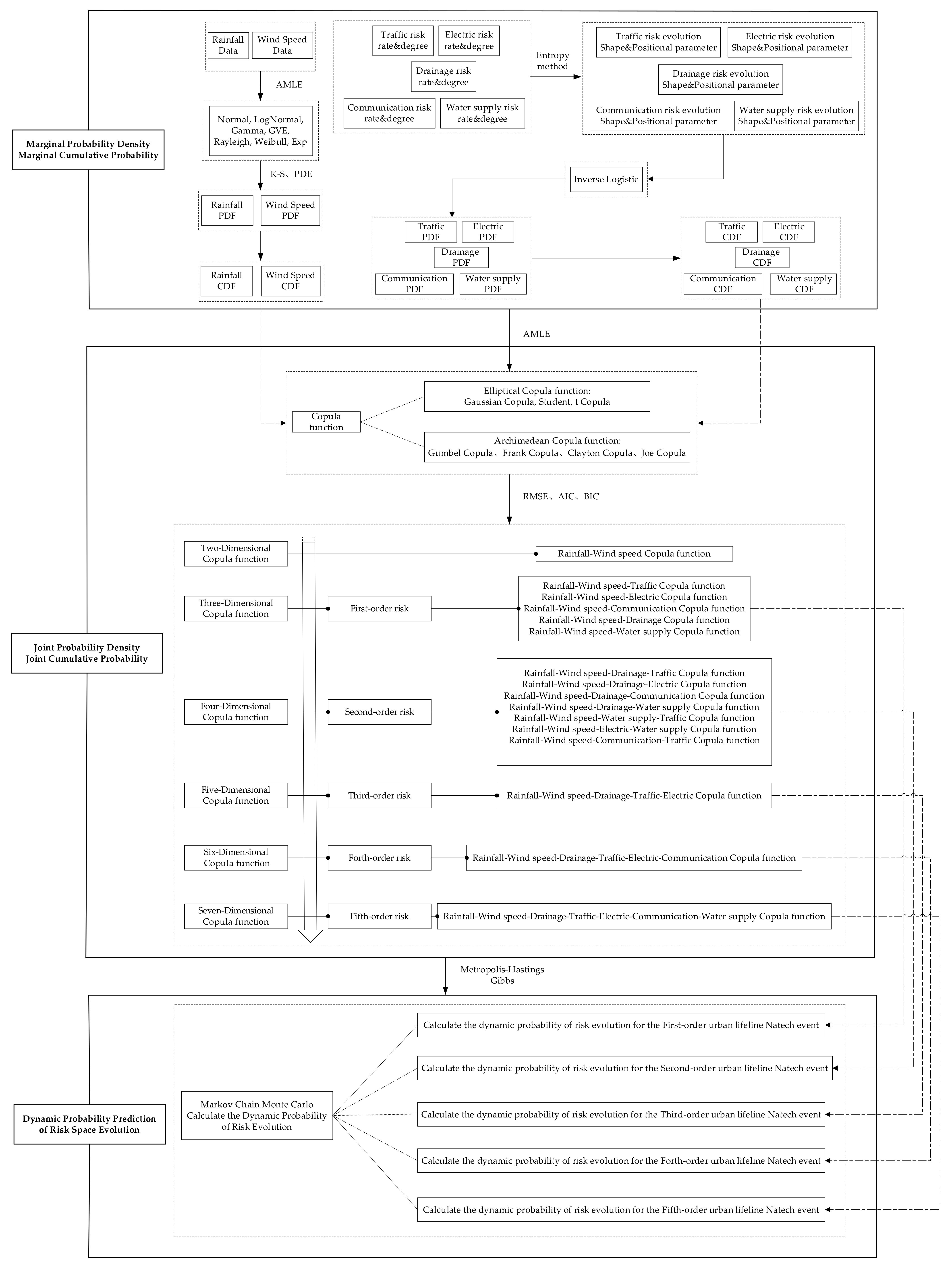
Section 2: Analyze the risk evolution mechanism of urban lifeline Natech events from the perspective of spatial evolution (parallel effects and synergistic effects). Section 3: Construct the MdC-MCMC model, which includes constructing the marginal probability distribution of natural hazard and urban lifeline risk evolution, and then construct the joint probability distribution function (MdC) of urban lifeline Natech event risk evolution. It is confirmed that the M-H algorithm and Gibbs sampling in the Monte Carlo (MC) method are used to construct the Markov Chain (MC) of urban lifeline Natech event risk evolution probability. Section 4: Apply the MdC-MCMC model, take the “July 20” extremely heavy rainstorm disaster in Zhengzhou in 2021 as an empirical case, use MATLAB R2020a software to fit the marginal probability distribution of natural hazard and urban lifeline risk evolution, and then fit the joint probability distribution function (MdC) of urban lifeline Natech event risk evolution, further clarifying the joint probability MCMC prediction process of urban lifeline Natech event risk evolution. Section 5: Conduct numerical simulations, where MATLAB R2020a software is used to visualize the marginal probability distribution of natural hazard and urban lifeline risk evolution, and then visualize the joint probability distribution (MdC) of urban lifeline Natech event risk evolution, and further visualize and quantify the joint probability of the urban lifeline Natech event risk evolution (MCMC). To provide a more intuitive display of the research content from Section 3 to Section 5, design a research framework as shown in Figure A1 (See Appendix A). Figure A1 shows in detail the 2-Dimensional (2-D) to 7-Dimensional (7-D) Copula functions and the 1st-order to 5th-order urban lifeline Natech event risk.

2. Mechanism of the Urban Lifeline Natech Event Risk Evolution

Urban lifelines (such as traffic, electric, drainage, etc.) exhibit multi-level and multi-dimensional coupling in an urban spatial layout, forming functional dependency systems through spatial interaction. Therefore, under the influence of the natural hazard chain and the domino effect risk transmission mechanism, the risk evolution of urban lifeline Natech events has significant spatial evolution attributes. The spatial evolution of the risk of urban lifeline Natech events is specifically manifested as parallel effects and synergistic effects [13,14,15]. Parallel effects refer to scenarios where natural hazards (e.g., rainstorms, gales) or risks associated with a specific urban lifeline (e.g., drainage) simultaneously impact other urban lifelines (e.g., traffic, water supply). Synergistic effects involve a single urban lifeline (e.g., traffic) being subjected to combined impacts from multiple natural hazards (e.g., rainstorms, gales) or risks from other urban lifelines (e.g., electric, drainage). The spatial evolution of Natech event risks in urban lifelines is reflected through changes in natural hazard warning colors (blue, yellow, orange, red), as illustrated in Figure 1. As warnings escalate from blue → yellow → orange → red, the risk evolves sequentially: latent risk (blue → yellow) → risk emergence (yellow → orange)→risk escalation (orange → red) → risk maturity (red → dark red). Consequently, quantifying the probability of risk evolution in urban lifeline Natech events has become a critical research focus.
In summarizing the above analysis, it is evident that the risk evolution process of urban lifeline Natech events exhibits significant complexity and randomness under the combined effects of parallel and synergistic mechanisms. This manifests as natural hazards or urban lifeline risks potentially transmitting to subsequent lifelines, forming risk transmission chains of varying orders. Therefore, to achieve the probabilistic prediction of risk evolution in urban lifeline Natech events, the following steps are critical: first, analyze the uncertainties in natural hazard risks and urban lifeline risks; second, examine the complexities arising from joint natural hazard risks affecting different urban lifelines and their associated risk transmission chains. Finally, address the randomness inherent in diverse urban lifeline risks and transmission chains. Uncertainty is represented through marginal probability density distributions and cumulative probability distributions, while complexity is captured via joint probability density and cumulative distributions. Randomness, meanwhile, is modeled through joint probability density forecasting and cumulative probability predictions.

3. Design and Methodology of the Urban Lifeline Natech Event Risk Evolution Probability

Firstly, the marginal probability distribution function of the natural hazard and urban lifeline risks evolution is fitted. Then, based on the marginal probability distribution function, the joint probability distribution function (MdC) for the risk evolution of the urban lifeline Natech event is constructed. Finally, based on the joint probability distribution function of risk evolution (MdC), the M-H algorithm and Gibbs sampling are used to construct a Markov Chain Monte Carlo (MCMC) model to achieve joint probability prediction of urban lifeline Natech event risk evolution.

3.1. Marginal Probability Distribution Function of Risk Evolution

The marginal probability distributions of risk evolution contribute to understanding the behavioral characteristics of individual variables within multi-dimensional random variables [16,17], forming a foundational basis for constructing the joint probability distribution function of urban lifeline Natech event risk evolution in subsequent analyses.

3.1.1. Marginal Probability Distribution of Natural Hazard Risk Evolution

The occurrence and development of natural hazards are characterized by uncertainty, making it challenging to assume they conform to a specific parametric distribution [18]. According to previous research on the evolution of natural hazard risks, functions such as the Normal distribution [19], Log-Normal distribution [20], Rayleigh distribution [21], Gamma distribution [22], Generalized Extreme Value (GEV) distribution [23], Weibull distribution [24], and Exponential (Exp) distribution [25] were usually employed to fit natural hazard data. Additionally, based on goodness-of-fit tests, the optimal fitting function was selected.
The Marginal Probability Density Function (PDF) of natural hazard risk evolution, Normal distribution:
u x = 1 2 π σ exp − x − μ 2 2 σ 2
where μ ∈ (−∞, +∞), σ > 0, x is natural hazard data such as Rainfall and Wind speed.
The Marginal Probability Density Function (PDF) of natural hazard risk evolution, Log-Normal distribution:
u x = 1 2 π σ x exp − ln x − μ 2 2 σ 2
where μ ∈ (−∞, +∞), σ > 0, x is natural hazard data such as Rainfall and Wind speed.
The Marginal Probability Density Function (PDF) of natural hazard risk evolution, Rayleigh distribution:
u x = x σ 2 exp − x 2 2 σ 2
where σ > 0, x is natural hazard data such as Rainfall and Wind speed.
The Marginal Probability Density Function (PDF) of natural hazard risk evolution, Gamma distribution:
u x = x α − 1 β α Γ α exp − x β
where α > 0, β > 0, x is natural hazard data such as Rainfall and Wind speed.
The Marginal Probability Density Function (PDF) of natural hazard risk evolution, GEV distribution:
u x = 1 β exp − 1 + α x − γ β − 1 α 1 + α x − γ β − 1 α − 1
where α ∈ (−∞, +∞), β > 0, γ ∈ (−∞, +∞), x is natural hazard data such as Rainfall and Wind speed.
The Marginal Probability Density Function (PDF) of natural hazard risk evolution, Weibull distribution:
u x = α β x β α − 1 exp − x β α
where α > 0, β > 0, x is natural hazard data such as Rainfall and Wind speed.
The Marginal Probability Density Function (PDF) of natural hazard risk evolution, Exp distribution:
u x = λ exp − λ x
where λ > 0, x is natural hazard data such as Rainfall and Wind speed.
The Marginal Cumulative Probability Distribution (CDF) of natural hazard risk evolution:
U x = ∫ 0 x u x d x
where U(x) is the cumulative probability of natural hazard risk, and u(x) is the probability density of natural hazard risk.

3.1.2. Marginal Probability Distribution of Urban Lifeline Risk Evolution

The “Gray Rhino” event has high probability, predictability, and high-risk characteristics, but is often overlooked due to cognitive limitations. When accumulated to a certain extent, it may trigger a systemic crisis. The “Black Swan” event has low probability, unpredictability, and high impact characteristics, usually triggered by small disturbances within complex systems, leading to chain reactions and huge impacts. If the “Gray Rhino” event is ignored or mishandled for a long time, its risk accumulation may break through a critical point, triggering unpredictable chain reactions and transforming into a “Black Swan” event. Risk accumulation is the intrinsic driving force behind the evolution of the “Gray Rhino” event into a “Black Swan” event, with critical point breakthroughs being key, and internal system vulnerabilities and external environmental changes being triggering factors. The process of the “Gray Rhino” event transforming into a “Black Swan” event follows three stages of the reverse S-shaped curve: slow growth, rapid growth, and stability. In scenarios where cognitive biases are coupled with risk interactions, it is conventionally perceived from a local and/or short-term perspective that there exists an inverse correlation between the level of risk evolution and its probability. Specifically, higher levels of risk evolution are typically associated with lower probabilities of occurrence, following the pattern of transition from “Gray Rhino” events to “Black Swan” events [26]. Consequently, it is hypothesized that the probability of risk evolution decreases nonlinearly as the level of risk evolution escalates [27,28].
In urban lifeline Natech events, the accumulation of risks constitutes a complex process involving the interaction of multiple factors, such as the intensity of natural disasters, the vulnerability and interdependence of urban lifelines. The risk accumulation trajectory of urban lifeline Natech events resembles “Gray Rhino” phenomena—characterized by high probability, predictability, and significant risk potential—yet remains frequently underestimated. When risks accumulate beyond critical thresholds, they may precipitate systemic crises. Conversely, the outbreak of risks in urban lifeline Natech events mirrors “Black Swan” characteristics: low probability, unpredictability, and severe impact. Under natural disaster scenarios, these outbreaks are typically triggered by perturbations in vulnerability and interdependence mechanisms, thereby initiating a domino effect; therefore, assuming a reverse S-shaped relationship between the probability of urban lifeline risk evolution and the risk evolution level, that is, following a reverse logistic distribution [29].
As depicted in Figure 1, the risk evolution levels of urban lifelines are categorized into blue, yellow, orange, red, and dark red, with deeper hues signifying higher risk evolution levels. Urban lifelines at elevated risk evolution levels must concurrently satisfy stringent conditions such as extreme natural hazard intensities, high vulnerability of the urban lifelines, and strong interconnectivity among them, making the simultaneous fulfillment of these criteria less probable. When the risk evolution level of urban lifelines is low, the rate of decrease in its evolution probability is relatively gradual; as the risk evolution level ascends to a certain threshold, the rate of probability decline accelerates; however, when the risk evolution level further escalates to higher tiers, this decrement rate decelerates once again.
The Marginal Probability Density Function (PDF) of urban lifeline risk evolution, Reverse Logistic distribution:
v x = 1 1 + e 1 ξ x → − 0.5 + ζ , x → = x 1 + x
where v(x) represents the marginal probability density of urban lifeline risk evolution; x → is the urban lifeline risk level (0~0.2 is blue risk, 0.2~0.4 is yellow risk, 0.4~0.6 is orange risk, 0.6~0.8 is red risk, and 0.8~1 is dark red risk); x ∈ (0, +∞); 1 ξ denotes the shape parameter for the marginal probability change in urban lifeline risk evolution, calculated based on the risk rate of urban lifeline Natech events [12]; and ζ represents the variation in the location parameter for the marginal probability change in urban lifeline risk evolution, calculated based on the risk degree of urban lifeline Natech events [12].
The Marginal Cumulative Probability (CDF) distribution of urban lifeline risk evolution.
V x = ∫ 0 x v x d x

3.1.3. Marginal Probability Parameter Estimation and Goodness-of-Fit Test of Risk Evolution

  • Parameter Estimation Method
The Maximum Likelihood Estimation method (MLE) estimates the parameters of a probability distribution by maximizing the likelihood of observing the given data [30]. Taking the Gamma distribution as an example, suppose a sample of natural hazard data is x1, x2, …, xn, xi ∈ [0, +∞). The maximum likelihood function is
M x 1 , x 2 , … , x n ; α , β = 1 Γ α β α n Π x i i = 1 n α − 1 e − 1 β ∑ i = 1 n x i
Taking the logarithm of both sides of the above equation yields the maximum likelihood function:
ln M x 1 , x 2 , … , x n ; α , β = − n ln Γ β − n β ln α + β − 1 ∑ n = 1 n x i − 1 α ∑ n = 1 n x i
Differentiating with respect to ln M x 1 , x 2 , … , x n ; α , β , yielding
f 1 x 1 , x 2 , … , x n ; α , β = ∂ ln x 1 , x 2 , … , x n ; α , β ∂ α f 2 x 1 , x 2 , … , x n ; α , β = ∂ ln x 1 , x 2 , … , x n ; α , β ∂ β
By setting f 1 x 1 , x 2 , … , x n ; α , β = 0 f 2 x 1 , x 2 , … , x n ; α , β = 0 , the parameters α and β of the distribution function for the marginal probability density of natural hazard risk evolution can be calculated.
2.
Goodness-of-Fit Test Methods
The Probability Distribution Error (PDE) [31] and Kolmogorov–Smirnov (K-S) test [32] were employed to evaluate the goodness-of-fit of the marginal probability density distribution function for natural hazard risk evolution. Smaller PDE and D-values indicate better fit performance.
The Probability Distribution Error (PDE):
P D E = 1 n ∑ i = 1 n E n x i − T n x i E n x i × 100 %
The K-S test:
D = max T n x i − E n x i
where En(xi) is the empirical distribution function of a certain natural hazard dataset, Tn(xi) is the theoretical distribution function of the same dataset, and n represents the sample size of the data. In the K-S test, if the measured statistic D is less than D (n, p) and its corresponding probability p-value is greater than the established confidence level (usually taken as 0.05), then the hypothesis is accepted, that is, the fitted natural disaster marginal probability distribution follows the theoretical distribution [33].

3.2. Joint Probability Distribution Function of Risk Evolution

Copula functions originate from Sklar’s theorem, which posits that for a joint distribution of N variables, it can be decomposed into the marginal distributions of the N variables and one Copula function, thereby separating the uncertainty and coupling nature of the variables. The uncertainty is characterized by the marginal distributions, while the coupling properties are described by the Copula function [34]. A Copula function links the marginal distributions of multiple uncertain variables into a joint distribution function to characterize the correlation structure between variables [35]. The risk evolution of urban lifeline Natech events arises from the combined effects of multiple natural hazards on various urban lifeline systems, as well as the interactions and mutual influences among these lifelines. Copula functions can capture the correlations between natural hazards and urban lifelines, providing a foundation for subsequent quantitative predictions of risk evolution probabilities.

3.2.1. Two-Dimensional Joint Probability Distribution of Risk Evolution

Copula functions include two common types: Elliptical Copula functions and Archimedean Copula functions [36]. Elliptical Copula functions comprise the Gaussian Copula [37] and t-Copula [38], which can capture symmetric correlations between marginal probability distributions. Archimedean Copula functions include the Gumbel Copula [39], Clayton Copula [40], Frank Copula [41], and Joe Copula [42]. Among them, Gumbel Copula, Joe Copula, and Clayton Copula can capture asymmetries in correlations from upper-tail or lower-tail perspectives, while Frank Copula exhibits symmetry. Let u1 and u2 represent the marginal probability distributions of risk evolution.
Two-Dimensional Risk Evolution Joint Probability Density Distribution (PDF) Gaussian Copula Function:
C Ga , θ u 1 , u 2 = 1 1 − θ 2 exp − θ 1 − θ 2 Φ − 1 u 1 , u 2
where θ is the fitting parameter of the Gaussian Copula function, where θ ∈ (−1, 1); Φ−1(·) denotes the inverse cumulative distribution function of the standard normal distribution.
Two-Dimensional Risk Evolution Joint Probability Density (PDF) Distribution t-Copula Function:
C t , θ , k u 1 , u 2 = Γ k + 2 2 π k Γ k 2 1 − θ 2 1 + t k − 1 u 1 2 + t k − 1 u 2 2 − 2 θ t k − 1 u 1 t k − 1 u 1 k 1 − θ 2 − k + 2 2
where θ is the fitting parameter of the t-Copula function, and where θ ∈ (−1, 1); t−1k(·) denotes the inverse cumulative distribution function of the standard t-distribution with degree of freedom k, k > 0.
Two-Dimensional Risk Evolution Joint Probability Density (PDF) Distribution Gumbel Copula Function:
C Gu , θ u 1 , u 2 = 1 u 1 u 2 − ln u 1 θ + − ln u 2 θ − 2 θ − 1 − ln u 1 θ + − ln u 2 θ 1 θ + θ − 1 − ln u 1 θ + − ln u 2 θ 1 θ − 1
where θ is the fitting parameter of the Gumbel Copula function, θ ∈ [1, +∞).
Two-Dimensional Risk Evolution Joint Probability Density (PDF) Distribution Frank Copula Function:
C Fr , θ = θ exp − θ u 1 + u 2 1 + exp − θ u 1 + exp − θ u 2 − 2 exp − θ exp − θ − 1 1 + exp − θ u 1 − 1 exp − θ u 2 − 1 exp − θ − 1 2
where θ is the fitting parameter of the Frank Copula function, θ ≠ 0.
Two-Dimensional Risk Evolution Joint Probability Density (PDF) Distribution Clayton Copula Function:
C Cl , θ u 1 , u 2 = 1 u 1 u 2 u 1 − θ + u 2 − θ − 1 − 1 θ θ θ + 1 u 1 − θ + u 2 − θ − 1 + θ
where θ is the fitting parameter of the Clayton Copula function, θ ∈ (0, +∞).
Two-Dimensional Risk Evolution Joint Probability Density (PDF) Distribution Joe Copula Function:
C Jo , θ u 1 , u 2 = θ 1 − u 1 θ − 1 1 − u 2 θ − 1 u 1 u 2 1 − 1 − u 1 θ 1 − 1 − u 2 θ 1 θ − 1 1 + θ − 1 1 − 1 − u 1 θ 1 θ 1 − 1 − u 2 θ 1 θ
where θ is the fitting parameter of the Joe Copula function, θ ∈ (1, +∞).

3.2.2. Three-Dimensional to 7-D Joint Probability Distribution of Risk Evolution

The joint probability density distribution of risk evolution for urban lifeline Natech events is a MdC function based on 2-D Copula functions. When the types of variables (natural hazards, urban lifelines) significantly increase, the flexibility and accuracy of the above-mentioned 2-D Copula functions will be limited to a certain extent. For the risk evolution of urban lifeline Natech events, the correlation between natural hazards and different urban lifelines varies, and as the risk propagates among urban lifelines, the correlation also gradually changes. By constructing an asymmetric MdC function, the correlation among the characteristic variables of the risk evolution of urban lifeline Natech events can be described. At this time, hierarchical Copula [43,44,45,46] can describe the correlation among the characteristic variables in the process of risk evolution of urban lifeline Natech events through fully nested or partially nested methods, thereby breaking the limitation of the increase in variable dimensions on the flexibility and accuracy of the Copula function. The following is the construction of the joint probability distribution function for the risk evolution of urban lifeline Natech events using a fully nested method.
Three-Dimensional Risk Evolution Joint Probability Density (PDF) Distribution Copula function:
C 2 u 1 , u 2 , v 1 ; θ 1 , θ 2 = C 2 C 1 u 1 , u 2 ; θ 1 , v 1 ; θ 2
Four-Dimensional Risk Evolution Joint Probability Density (PDF) Distribution Copula function:
C 3 u 1 , u 2 , v 1 , v 2 ; θ 1 , θ 2 , θ 3 = C 3 C 2 C 1 u 1 , u 2 ; θ 1 , v 1 ; θ 2 , v 3 ; θ 3
Five-Dimensional Risk Evolution Joint Probability Density (PDF) Distribution Copula function:
C 4 u 1 , u 2 , v 1 , v 2 , v 3 ; θ 1 , θ 2 , θ 3 , θ 4 = C 4 C 3 C 2 C 1 u 1 , u 2 ; θ 1 , v 1 ; θ 2 , v 3 ; θ 3 , v 4 ; θ 4
Extending this logic, the j-D Risk Evolution Joint Probability Density (PDF) Distribution Copula function is derived.

3.2.3. Joint Probability Parameter Estimation and Goodness-of-Fit Test of Risk Evolution

1.
Parameter Estimation Methods
Similarly to Section 3.1, the MLE is employed to estimate the parameter values of the Multi-dimensional Copula function [47]. The joint probability density distribution of risk evolution for natural hazards and urban lifelines X1, X2, …, Xj is expressed as C F X 1 x 1 , F X 2 x 2 , … , F X j x j , u 1 = F X 1 x 1 , u 2 = F X 2 x 2 , … , u j = F X j x j , where θ represents the parameter values of the Multi-dimensional Copula function. The maximum likelihood function over the risk evolution space of u 1 , u 2 , … , u j is as follows:
M θ = ∏ i = 1 j C u i 1 , u i 2 , … , u i j ; θ
The logarithm is taken of both sides of the equation, yielding
ln M θ = ∑ i = 1 j ln C u i 1 , u i 2 , … , u i j ; θ
Taking the derivative with respect to ln M θ , yielding
f u i 1 , u i 2 , … , u i j ; θ = ∂ n C u i 1 , u i 2 , … , u i j ; θ ∂ u 1 ∂ u 2 … ∂ u j
By setting f u i 1 , u i 2 , … , u i j ; θ = 0 , the parameter θ values of the multivariate Copula function for the joint probability density distribution of risk evolution in urban lifeline Natech events are calculated.
2.
Goodness-of-Fit Evaluation Method
The goodness-of-fit evaluation of the MdC function for the joint probability density distribution of risk evolution in urban lifeline Natech events is conducted using the Root Mean Square Error (RMSE) [48], Akaike Information Criterion (AIC) [49], and Bayesian Information Criterion (BIC) [50]. Smaller values of RMSE, AIC, and BIC indicate better fit performance.
R M S E = 1 j ∑ i = 1 j E x i 1 , x i 2 , … , x i j − T x i 1 , x i 2 , … , x i j 2
A I C = j ln 1 j ∑ i = 1 j E x i 1 , x i 2 , … , x i j − T x i 1 , x i 2 , … , x i j 2 + 2 m
B I C = j ln 1 j ∑ i = 1 j E x i 1 , x i 2 , … , x i j − T x i 1 , x i 2 , … , x i j 2 + m ln j
where E(xi1, xi2, …, xij) represents the empirical joint probability frequency value of risk evolution for urban lifeline Natech events; T(xi1, xi2, …, xij) represents the theoretical joint probability frequency value of risk evolution for urban lifeline Natech events; j denotes the dimension of the joint probability distribution function for risk evolution of urban lifeline Natech events; and m is the number of model parameters.

3.3. Joint Probability Prediction Method of Risk Evolution

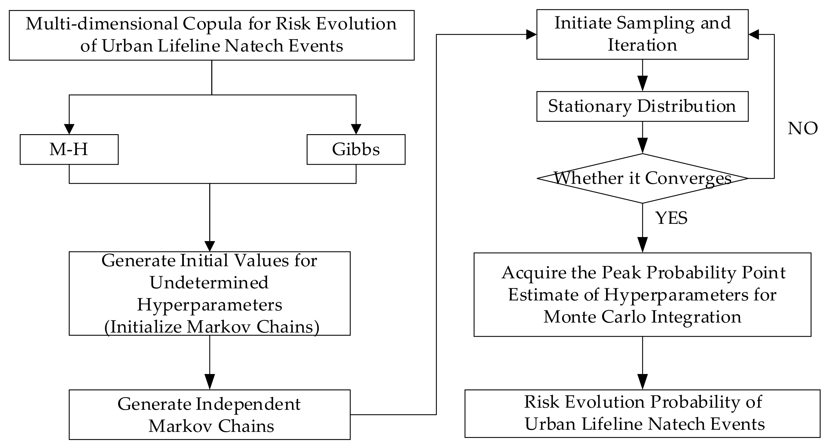
The core principle of MCMC involves constructing an independent Markov chain, which through iterative operations converges to a stationary distribution. This stationary distribution aligns with the target distribution, enabling the application of Monte Carlo integration on effective samples from the stationary distribution [34,51]. As a simulation-based approach for high-dimensional integration, MCMC methodology effectively addresses multi-dimensional, complex, and dynamic risk evolution probability distributions in urban lifeline Natech events, facilitating the quantitative predictions of such risks. In this context, the Metropolis–Hastings (M-H) algorithm and Gibbs sampling are employed to construct Markov Chains representing the risk evolution probabilities of urban lifeline Natech events, while the Gelman–Rubin diagnostic is utilized to assess the convergence of these chains.

3.3.1. M-H Algorithm

The Metropolis–Hastings algorithm, proposed by Metropolis et al. and generalized by Hastings et al., derives the stationary distribution by employing the detailed balance condition. The distribution of the required importance samples corresponds to the desired stationary distribution, making it a classic MCMC method [52].
Select the risk evolution transition function q x ; x r − 1 and initial values x 0 for the urban lifeline Natech event. Assume that the parameter values at the beginning of the r-th iteration are x r − 1 , then the iteration process is as follows: draw candidate values x ′ from q x ; x r − 1 ; calculate the acceptance probability p x r − 1 , x ′ = min π x r − 1 ; x ′ π x r − 1 q x ′ ; x r − 1 , 1 ; update the parameter to the candidate value x r = x ′ with probability p x r − 1 , x ′ , or retain the current value x r = x r − 1 with probability 1 − p x r − 1 , x ′ ; and repeat the above steps g times to obtain a stationary distribution sample x 1 , x 2 , … , x g of the urban lifeline Natech event risk evolution. Based on the stationary distribution sample, compute the moments of the stationary distribution and apply Monte Carlo integration for probabilistic prediction of the risk evolution.

3.3.2. Gibbs Sampling

Gibbs sampling, proposed by Gelman, possesses the capability to generate conditionally independent sample sequences in multivariate distributions, effectively approximating the overall distribution. It excels at addressing challenges involving high-dimensional probability distributions and stands as a broadly applicable MCMC method [53].
Assume an arbitrary initial vector x 0 = x 1 0 , x 2 0 , … , x l 0 for the risk evolution of urban lifeline Natech events; draw sample x 1 1 from π x 1 x 2 0 , … , x l 0 ; draw sample x 2 1 from π x 2 x 1 0 , … , x l 0 ; draw sample x k 1 from π x k x 1 1 , x 2 1 , x k − 1 1 , x k − 1 0 , … , x l 0 ; and draw sample x l 1 from π x l x 1 1 , x 2 1 , … , x l − 1 1 to complete the x 0 → x 1 transition. After g iterations, a stationary distribution sample x 1 , x 2 , … , x g of the risk evolution for urban lifeline Natech events can be obtained. Based on the stationary distribution sample, the moments of the stationary distribution can be calculated, and Monte Carlo integration can be used for the probabilistic prediction of the risk evolution.

3.3.3. Convergence Test

A Markov chain refers to a stochastic process in which the probability of state transitions at a given moment depends solely on the previous state and exists within a discrete index set and state space, characterized by convergence and sample independence [54,55]. The Gelman–Rubin diagnostic method [56] is employed to assess the convergence of the Markov Chains. When z Markov Chains with dispersed initial values are run in parallel until reaching a converged state, their inferential results should exhibit minimal discrepancy, with ratios approaching 1. First, relatively dispersed initial values are selected from the target distribution to establish z Markov Chains, each iterated 2g times. The results of the first g iterations are discarded, while the results of the last g iterations are retained and analyzed. Next, the variance E g between the g Markov Chains is calculated. Let the target statistic be e, and the value of e for the w-th sample in the y-th chain be denoted as e w y , then E g = 1 z − 1 ∑ y = 1 z 1 g ∑ w = g + 1 2 g e w y − 1 z ∑ y = 1 z 1 g ∑ w = g + 1 2 g e w y 2 . Subsequently, the intra-chain variance B is computed for individual Markov Chains, B = 1 z ∑ y = 1 z 1 g − 1 ∑ w = g + 1 2 g e w y − 1 g ∑ w = g + 1 2 g e w y 2 . Finally, a convergence diagnostic indicator C is constructed, C = g − 1 g B + 1 + 1 z E g B . When C > 1, the Markov Chains do not converge; when C ≈ 1, the Markov Chains are deemed to have converged.

4. Data and Result of the Urban Lifeline Natech Event Risk Evolution Probability

The “7·20” catastrophic rainstorm disaster in Zhengzhou, Henan Province, in 2021 was used as a case study for the empirical analysis of probabilistic models of risk evolution in urban lifeline Natech events. Natural hazard data, including Rainfall and Wind speed (72 sets of data) from 19 to 21 July 2021, were sourced from the “National Meteorological Science Data Center—Global Surface Weather Observation Dataset-Hourly Product”. The dataset directly provides the hourly observation data of rainfall and wind speed, without statistical conversion, and does not require resampling. The Investigation Report on the “7·20” Catastrophic Rainstorm Disaster in Zhengzhou, Henan Province” noted that “urban rainfall far exceeded drainage capacity, leading to severe flooding of residential communities and public facilities... with multiple areas experiencing disruptions in water supply, electric, communication, and road traffic.” From this, it can be inferred that the urban lifelines affected by the risks of rainfall and wind include traffic, electric, communication, drainage, and water supply. Meanwhile, risks are conducted among different urban lifelines, forming risk transmission chains, as illustrated in Figure 2. The evolution of heavy rainfall and wind constitutes the initial risk, with urban lifelines such as Traffic, Electric, Communication, Water supply, and Drainage initially impacted only by the Rainfall and Wind speed, evolving into a 1st-order risk transmission chain. Urban lifelines like Traffic, Electric, and Water supply may be affected by the combination of Rainfall, Wind, and Drainage issues, while Water supply and Communication may be influenced by the combination of Rainfall, Wind, and Electric outages, evolving into a 2nd-order risk transmission chain. Urban Electric may be impacted by the combined effects of Rainfall, Wind, Drainage problems, and Traffic disruptions, forming a 3rd-order risk transmission chain. Urban Communication may be affected by the cumulative impacts of Rainfall, Wind, Drainage failures, Traffic interruptions, and Electric outages, evolving into a 4th-order risk transmission chain. Urban Water supply may be influenced by the compounded effects of Rainfall, Wind, Drainage failures, Traffic disruptions, Electric outages, and Communication breakdowns, forming a 5th-order risk transmission chain.

4.1. Risk Evolution Marginal Probability Distribution Function Fitting

4.1.1. Marginal Probability Distribution Fitting of Natural Hazard Risk Evolution

The probability density and cumulative probability distribution of Rainfall and Wind risk evolution are crucial for understanding their intensity-frequency characteristics and mutual relationships. A 1 h Rainfall is suitable for analyzing the impact of a short-duration rainstorm on urban lifeline systems, making it ideal for immediate response and emergency disposal related to urban lifelines. A 3 h Rainfall applies to assessing risks posed by medium-to-short-duration continuous rainfall to urban lifeline systems, fitting well with localized emergency management and resource allocation within these networks. A 6 h Rainfall serves to evaluate risks associated with medium-to-long-duration sustained rainfall affecting urban lifeline systems, aligning effectively with risk assessment and long-term emergency management practices. A 12 h Rainfall is utilized for analyzing risks stemming from prolonged rainfall events on urban lifeline systems, corresponding closely with long-term planning and infrastructure development for urban lifelines. Notably, 3 h rainfall emerges as a relatively optimal metric, as it not only captures the persistence and cumulative effects of precipitation but also ensures comprehensiveness in risk analysis.
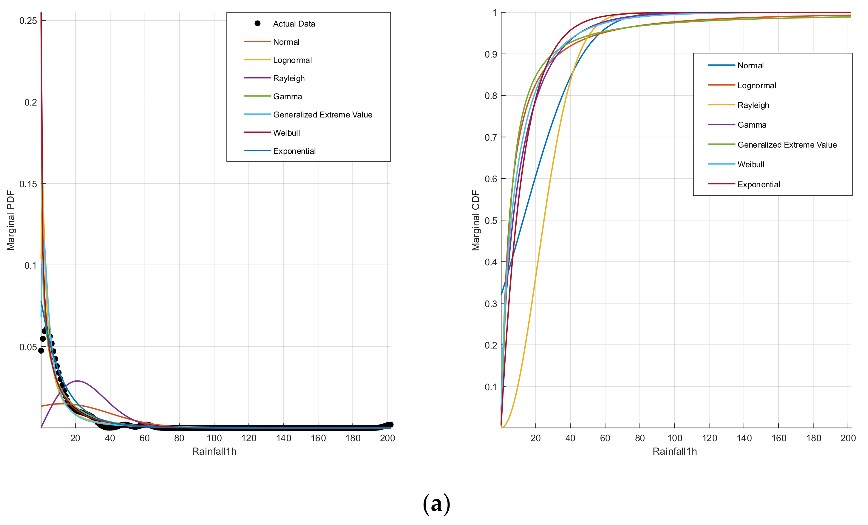
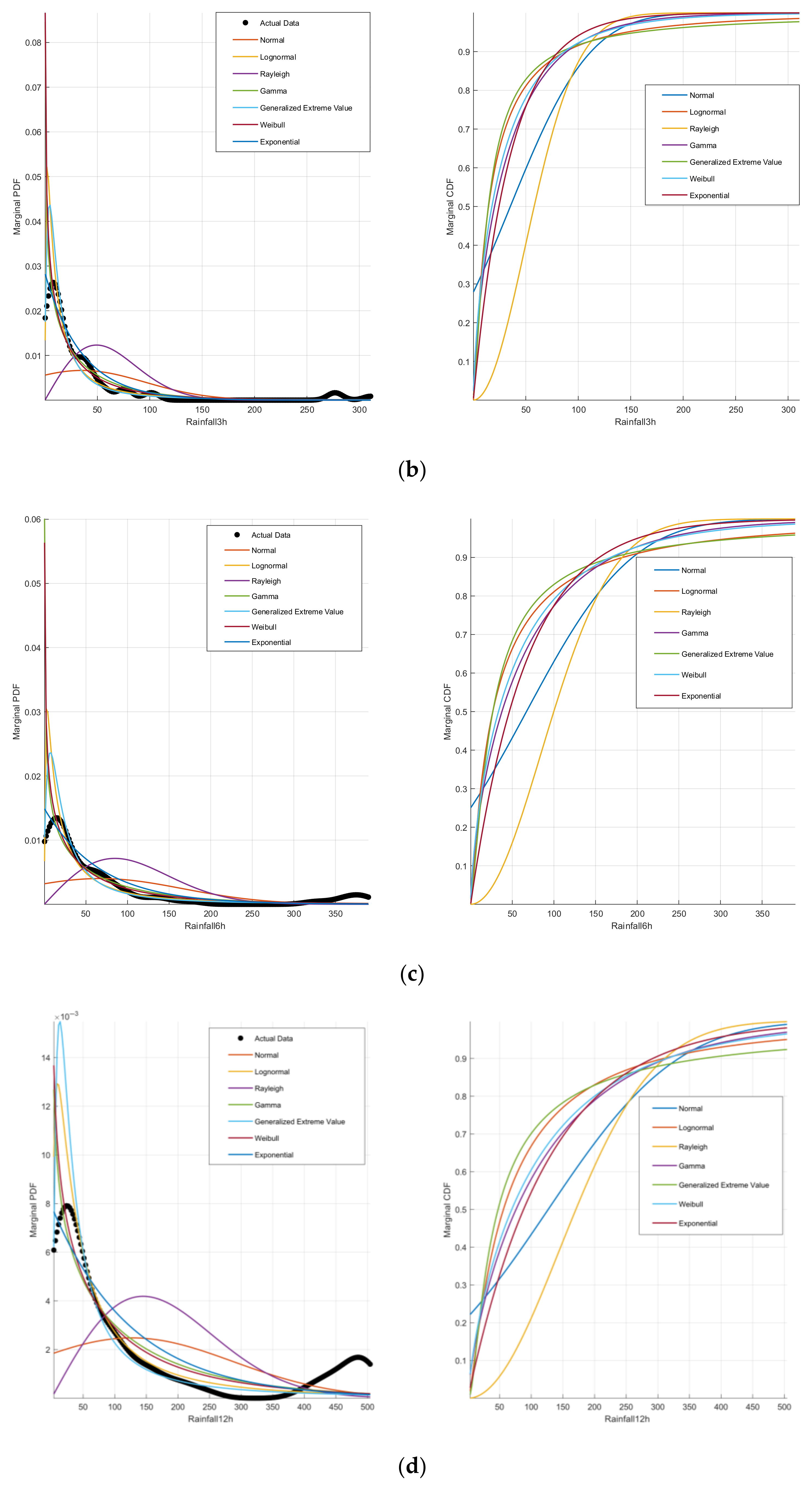
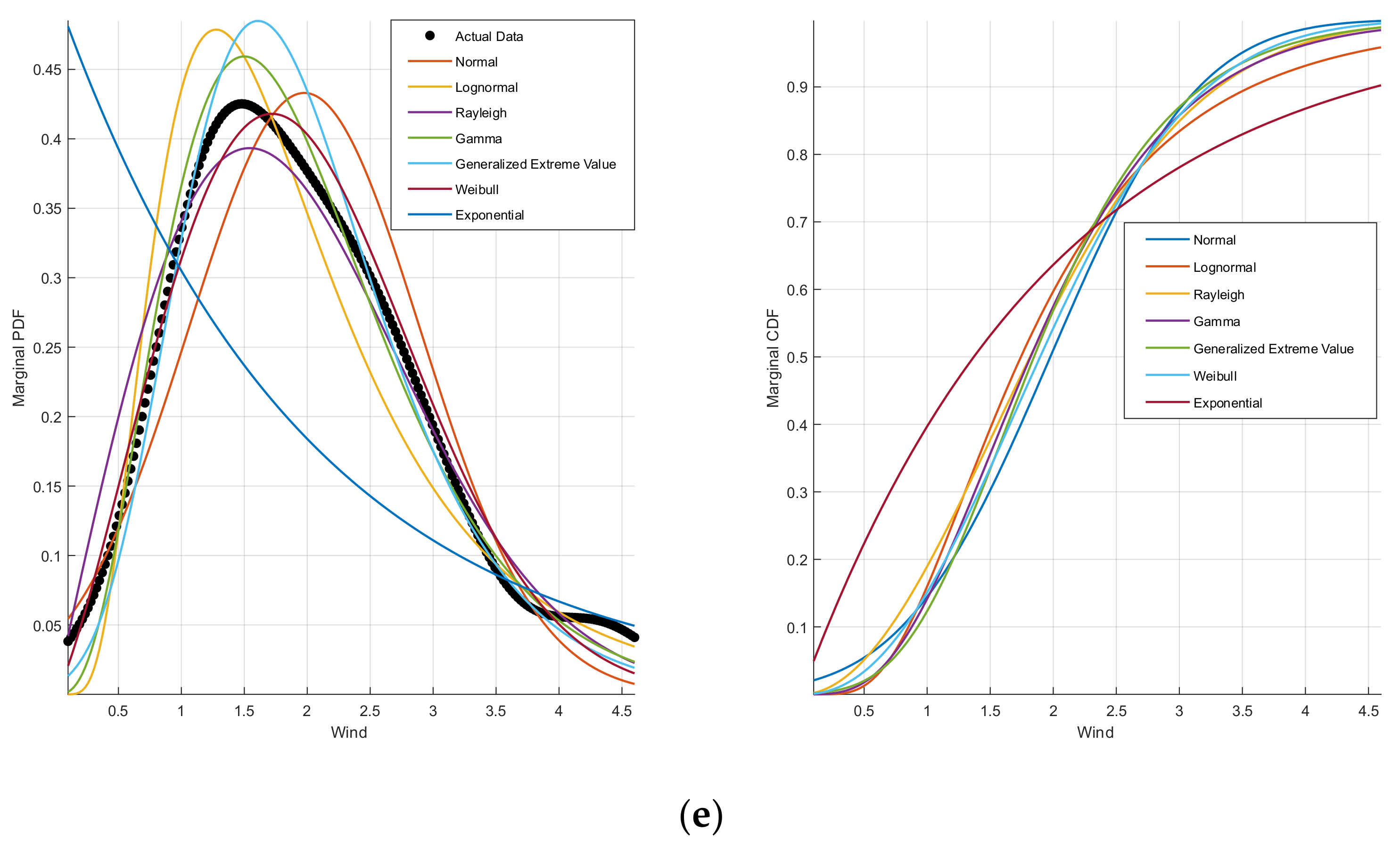
Table 1 provides detailed fitting results of marginal probability distributions for 1 h, 3 h, 6 h, and 12 h Rainfall as well as Wind speed under seven distribution types, including Normal, Log Normal, Gamma, GEV, Rayleigh, Weibull, and Exp distributions. The optimal distribution is selected based on the minimum sum of PDE and K-S test values. As shown in Table 1, the GEV distribution is identified as the optimal fit for 1 h, 6 h, and 12 h Rainfall risk evolution, while the Log Normal distribution best fits the 3 h Rainfall risk evolution. For Wind speed risk evolution, the Gamma distribution demonstrates the highest consistency. Figure 3 visualizes the probability density and cumulative probability distributions of Rainfall and Wind speed risk evolution. Figure 3a–d illustrates that Rainfall risk evolution exhibits a downward “C”-shaped probability density curve and an upward “C”-shaped cumulative probability curve, indicative of significant long-tailed effects. Notably, the 3 h Rainfall shows the highest peak density among all durations, suggesting the greatest hazard severity; thus, it is selected as a key variable for the subsequent joint probability analysis of risk evolution. Figure 3e reveals that Wind speed risk evolution follows an inverted “V”-shaped probability density curve and an “S”-shaped cumulative probability curve, with slow ascent in 0~1 m/s, rapid increase in 1~3.5 m/s, and gradual rise in 3.5~4 m/s intervals, demonstrating distinct platform effects.

4.1.2. Marginal Probability Distribution Fitting of Urban Lifelines Risk Evolution

Section 3.1.2 assumes an inverse S-shaped relationship between the probability evolution of urban lifeline Natech event risks and their corresponding risk levels, indicating adherence to an inverse Logistic distribution. To obtain the location and shape parameters required by Equation (9), draw upon the calculated risk velocity and severity metrics for urban lifeline Natech events from reference [12]. Using Z-score normalization and the Entropy method, comprehensive scores integrating risk velocity and severity are derived. These composite scores serve, respectively, as the shape and location parameters for the inverse Logistic function. The dataset employed in reference [12] utilizes textual data from “China’s Top Ten National Natural Disasters” and associated news reports. Event names were used as search keywords across publicly accessible online sources to identify textual descriptions of urban lifeline disruptions (including Traffic, Electric, Communications, Water supply, and Drainage interruptions) caused by natural disasters within news articles. Based on co-occurrence analysis, the Complex Network (CN)–System Dynamics (SD) integrated model was constructed to compute the risk velocity and severity metrics for urban lifeline Natech events.
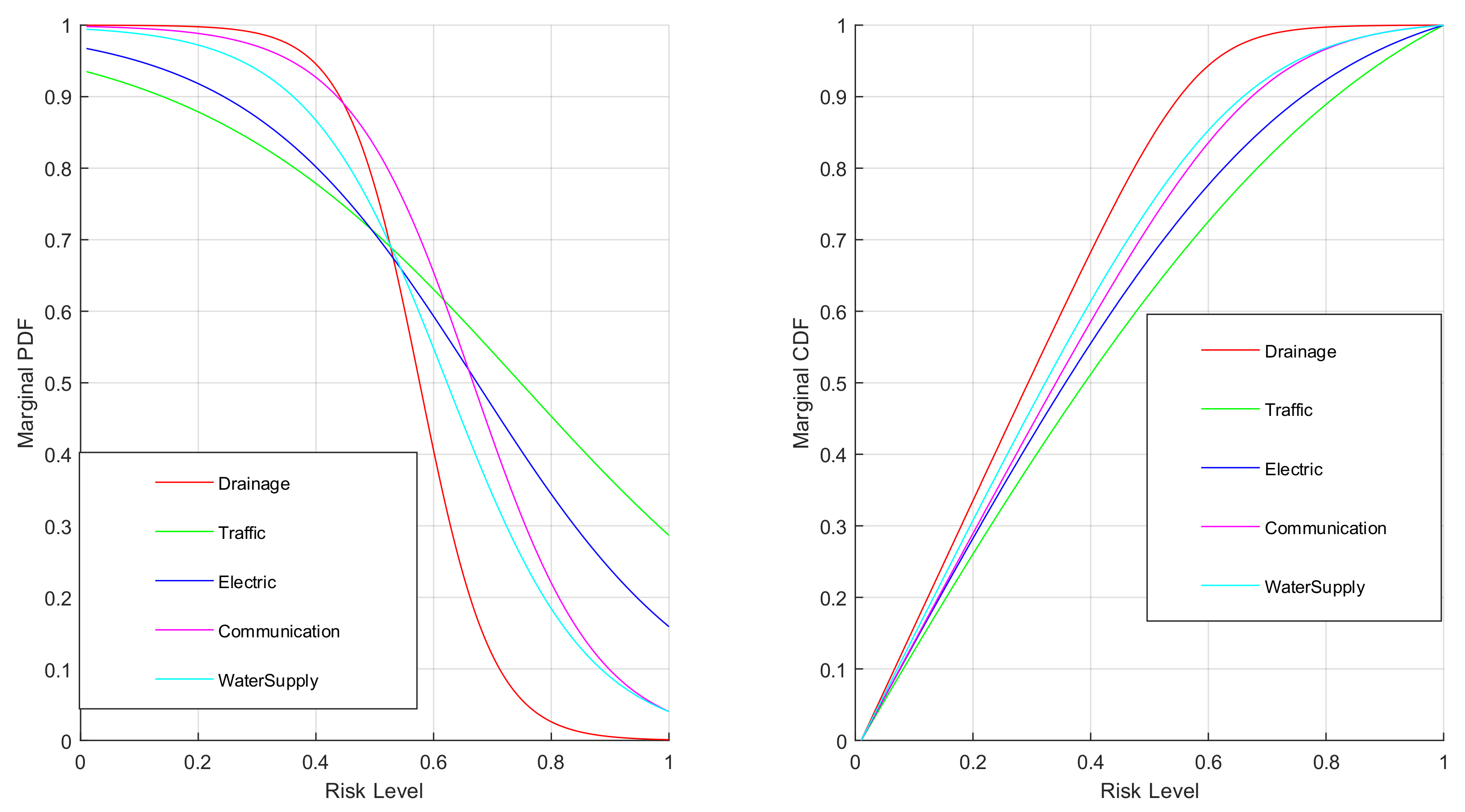
Figure 4 visualizes the distribution of probability density and cumulative probability for urban lifeline risk evolution. The probability density curve exhibits an inverted “S” shape, while the cumulative probability curve presents a “S” shape. From the probability density curve of urban lifeline risk evolution, in the 0~0.4 risk level interval, the evolutionary probability density ranks in descending order as Drainage > Communication > Water supply > Electric > Traffic. In the 0.7~1 risk level interval, the evolutionary probability density ranks in descending order as Traffic > Electric > Communication > Water supply > Drainage. In the 0.4~0.7 risk level interval, the evolutionary probability density shows complex and intertwined characteristics. From the cumulative probability curve of urban lifeline risk evolution, within the 0~1 risk level interval, the evolutionary cumulative probability ranks in descending order as Drainage > Water supply > Communication > Electric > Traffic.
Traffic system risk evolution probability density (PDF) distribution:
v x = 1 1 + e 1 0.2767 x − 0.5 + 0.2479
Electric system risk evolution probability density (PDF) distribution:
v x = 1 1 + e 1 0.1959 x − 0.5 + 0.1738
Communication system risk evolution probability density (PDF) distribution:
v x = 1 1 + e 1 0.1051 x − 0.5 + 0.1671
Water supply system risk evolution probability density (PDF) distribution:
v x = 1 1 + e 1 0.1190 x − 0.5 + 0.1229
Drainage system risk evolution probability density (PDF) distribution:
v x = 1 1 + e 1 0.0618 x − 0.5 + 0.0763

4.2. Risk Evolution Joint Probability Distribution Function Fitting

4.2.1. Joint Probability Distribution Fitting of Natural Hazard Risk Evolution

Table 2 provides a detailed comparison of the Gaussian Copula, t Copula, Gumbel Copula, Clayton Copula, Frank Copula, and Joe Copula functions for fitting the joint probability distribution of 3 h Rainfall and Wind speed risk evolution (2-D Copula function). The evaluation criteria include the RMSE, AIC, and BIC test values, along with the parameter estimates for each Copula function. The optimal Copula function is selected based on the minimal sum of RMSE, AIC, and BIC values. As shown in Table 2, the Gumbel Copula is identified as the best-fitting function for modeling the joint probability distribution of 3 h Rainfall-Wind speed risk evolution, indicating a significant upper tail dependence in their risk evolution.

4.2.2. Joint Probability Distribution Fitting of Natural Hazard-Urban Lifelines Risk Evolution

(1) Based on the risk transmission chain relationships of the urban lifelines characterized in Figure 2, the joint probability distribution functions for the 3 h Rainfall, Wind speed, and the risk evolution of Traffic, Electric, Communication, Water supply, and Drainage systems were fitted (3-D Copula function). Table 3 provides a detailed comparison of the Gaussian Copula, t Copula, Gumbel Copula, Clayton Copula, Frank Copula, and Joe Copula functions for fitting the above 1st-order risk evolution joint probability distributions. The evaluation criteria include RMSE, AIC, and BIC test values, as well as the parameter estimates for each Copula function. The optimal Copula function was selected based on the minimum sum of RMSE, AIC, and BIC values. As shown in Table 3, the Gumbel Copula is identified as the optimal function for all the 1st-order risk evolution joint probability distributions, indicating a significant upper tail dependence characteristic in their risk evolution.
(2) Based on the risk transmission chain relationships of urban lifelines characterized in Figure 2, the joint probability distribution functions for the 2nd-order risk evolution of the following systems were fitted (4-D Copula function): 3 h Rainfall-Wind speed-Drainage-Traffic, 3 h Rainfall-Wind speed-Drainage-Electric, 3 h Rainfall-Wind speed-Drainage-Communication, 3 h Rainfall-Wind speed-Drainage-Water supply, 3 h Rainfall-Wind speed-Water supply-Traffic, 3 h Rainfall-Wind speed-Electric-Water supply, 3 h Rainfall-Wind speed-Communication-Traffic, and 3 h Rainfall-Wind speed-Electric-Communication. Table 4 provides a detailed comparison of the Gaussian Copula, t Copula, Gumbel Copula, Clayton Copula, Frank Copula, and Joe Copula functions for fitting the above 2nd-order risk evolution joint probability distributions. The evaluation criteria include RMSE, AIC, and BIC test values, as well as the parameter estimates for each Copula function. The optimal Copula function was selected based on the minimal sum of RMSE, AIC, and BIC values. As shown in Table 4, the Gumbel Copula is identified as the optimal function for all the 2nd-order risk evolution joint probability distributions, indicating a significant upper tail dependence characteristic in their risk evolution.
(3) Based on the risk transmission chain relationships of urban lifelines characterized in Figure 2, the joint probability distribution functions for the 3rd-order risk evolution of the system involving 3 h Rainfall-Wind speed-Drainage-Traffic-Electric were fitted (5-D Copula function). Table 5 provides a detailed comparison of the Gaussian Copula, t Copula, Gumbel Copula, Clayton Copula, Frank Copula, and Joe Copula functions for fitting the above 3rd-order risk evolution joint probability distributions. The evaluation criteria include RMSE, AIC, and BIC test values, as well as the parameter estimates for each Copula function. The optimal Copula function was selected based on the minimal sum of RMSE, AIC, and BIC values. As shown in Table 5, the Gumbel Copula is identified as the optimal function for all the 3rd-order risk evolution joint probability distributions, indicating a significant upper tail dependence characteristic in their risk evolution.
(4) Based on the risk transmission chain relationships of urban lifelines characterized in Figure 2, the joint probability distribution functions for the 4th-order risk evolution of the system involving 3 h Rainfall-Wind speed-Drainage-Traffic-Electric-Communication were fitted (6-D Copula function). Table 6 provides a detailed comparison of the Gaussian Copula, t Copula, Gumbel Copula, Clayton Copula, Frank Copula, and Joe Copula functions for fitting the above 4th-order risk evolution joint probability distributions. The evaluation criteria include RMSE, AIC, and BIC test values, as well as the parameter estimates for each Copula function. The optimal Copula function was selected based on the minimal sum of RMSE, AIC, and BIC values. As shown in Table 6, the Gumbel Copula is identified as the optimal function for all the 4th-order risk evolution joint probability distributions, indicating a significant upper tail dependence characteristic in their risk evolution.
(5) Based on the risk transmission chain relationships of urban lifelines characterized in Figure 2, the joint probability distribution functions for the 5th-order risk evolution of the system involving 3 h Rainfall-Wind speed-Drainage-Traffic-Electric-Communication-Water supply were fitted (7-D Copula function). Table 7 provides a detailed comparison of the Gaussian Copula, t Copula, Gumbel Copula, Clayton Copula, Frank Copula, and Joe Copula functions for fitting the above 5th-order risk evolution joint probability distributions. The evaluation criteria include RMSE, AIC, and BIC test values, as well as the parameter estimates for each Copula function. The optimal Copula function was selected based on the minimal sum of RMSE, AIC, and BIC values. As shown in Table 7, the Gumbel Copula is identified as the optimal function for all the 5th-order risk evolution joint probability distributions, indicating a significant upper tail dependence characteristic in their risk evolution.

4.3. Risk Evolution Joint Probability Prediction Process

Based on the joint probability distribution function of risk evolution for urban lifelines under Natech events, Markov Chains are generated using the M-H and Gibbs. Iterative operations are performed to obtain Markov Chains with stationary distributions. Monte Carlo integration is then applied to the states (stationary distribution samples) at each time step in the time series. This process ultimately achieves the prediction of risk evolution probabilities for urban lifeline Natech events, with the algorithmic workflow illustrated in Figure 5.

5. Visualization of the Urban Lifeline Natech Event Risk Evolution Probability

Using MATLAB 2020Ra software for numerical simulation of the joint probability distribution of 3 h Rainfall-Wind speed risk evolution during the “7·20” catastrophic rainstorm disaster in Zhengzhou in 2021, the complexity of risk evolution for urban lifeline Natech events can be visually represented intuitively; the joint probability distributions of risk evolution for 1st-order to 5th-order urban lifeline Natech events, along with the prediction results of risk evolution joint probability, can intuitively visualize the randomness of risk evolution for urban lifeline Natech events.
According to the optimal Copula function for the joint probability distribution of risk evolution in Section 4.2, the joint probability density function and joint cumulative distribution function of risk evolution are numerically simulated. The contour map of joint probability density for risk evolution reflects the distribution range of random variable combinations, with the shape and size indicating the correlation between random variables; a three-dimensional grid diagram can correspond to the probability density values of all random variable combinations, using color and numerical values to indicate the probability density of random variable combinations, with the extreme values at the endpoints reflecting the degree of mutual influence between them in terms of probability density. The contour map of joint cumulative probability of risk evolution reflects the cumulative probability value of random variable combinations falling within that region, with the steepness indicating the correlation between random variables; a three-dimensional grid diagram can correspond to the cumulative probability values of all variable combinations, using color and numerical values to indicate the cumulative probability of random variable combinations, with the extreme values at the left and right endpoints reflecting the degree of mutual influence between them in terms of evolutionary probability.

5.1. Joint Probability Distribution of 3 h Rainfall-Wind Speed Risk Evolution

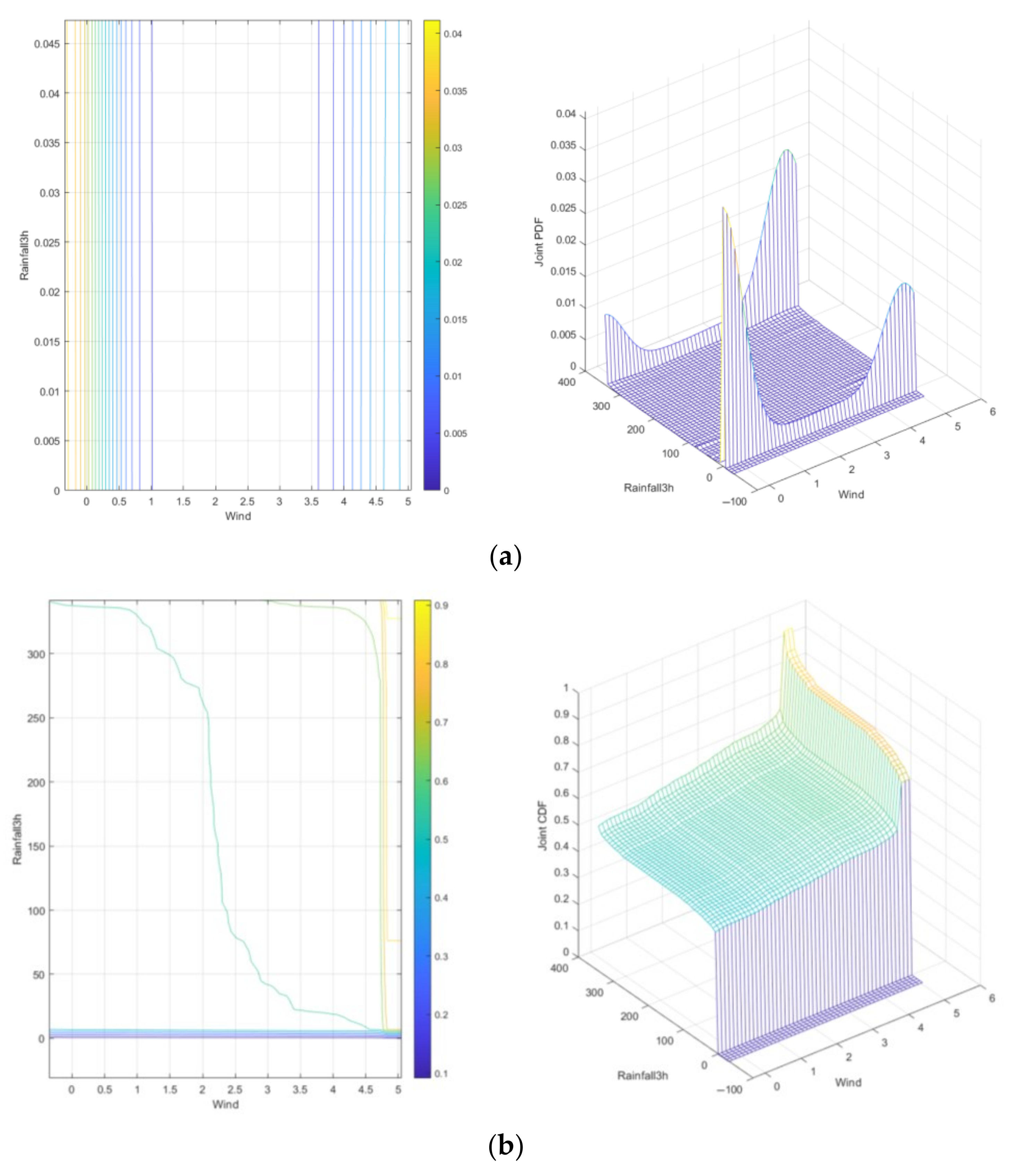
Based on the numerical simulation of the joint probability distribution of 3 h Rainfall-Wind speed risk evolution using the Gumbel Copula function, the joint probability density function and joint cumulative distribution function are obtained, as shown in Figure 6.
Based on Figure 3b, the analysis of Figure 6a reveals spatial heterogeneity in the joint probability density of 3 h Rainfall-Wind speed risk evolution. In the low-value domain of 3 h Rainfall-Wind speed, densely clustered contour lines and a prominent three-dimensional single-peak feature are observed, indicating concentrated low-risk regions with high probability density. As the risk value domain of 3 h Rainfall-Wind speed increases, the probability density attenuates significantly, and the contour lines become sparse, reflecting a sharp decline in probability density within high-risk domains. Analysis of Figure 6b demonstrates dynamic evolution in the joint cumulative probability of 3 h Rainfall-Wind speed risk. In the low-risk domain, steep cumulative probability gradients suggest that minor fluctuations in 3 h Rainfall or Wind speed could rapidly trigger threshold crossings. In contrast, gradients flatten in the high-risk domain, indicating saturation in risk accumulation. The low-risk domain exhibits strong tail correlations dominating risk coupling effects, whereas variable independence increases in the high-risk domain, revealing that the risk intensity of 3 h rainfall significantly surpasses that of Wind speed. The maximum probability point is a Rainfall of 341.9 mm/3 h and a Wind speed of 4.499 m/s, with a probability density of 0.02041.

5.2. Joint Probability Distribution of 3 h Rainfall-Wind Speed-Urban Lifeline Risk Evolution

5.2.1. Joint Probability Distribution of 3 h Rainfall-Wind Speed-Urban Lifeline 1st-Order Risk Evolution

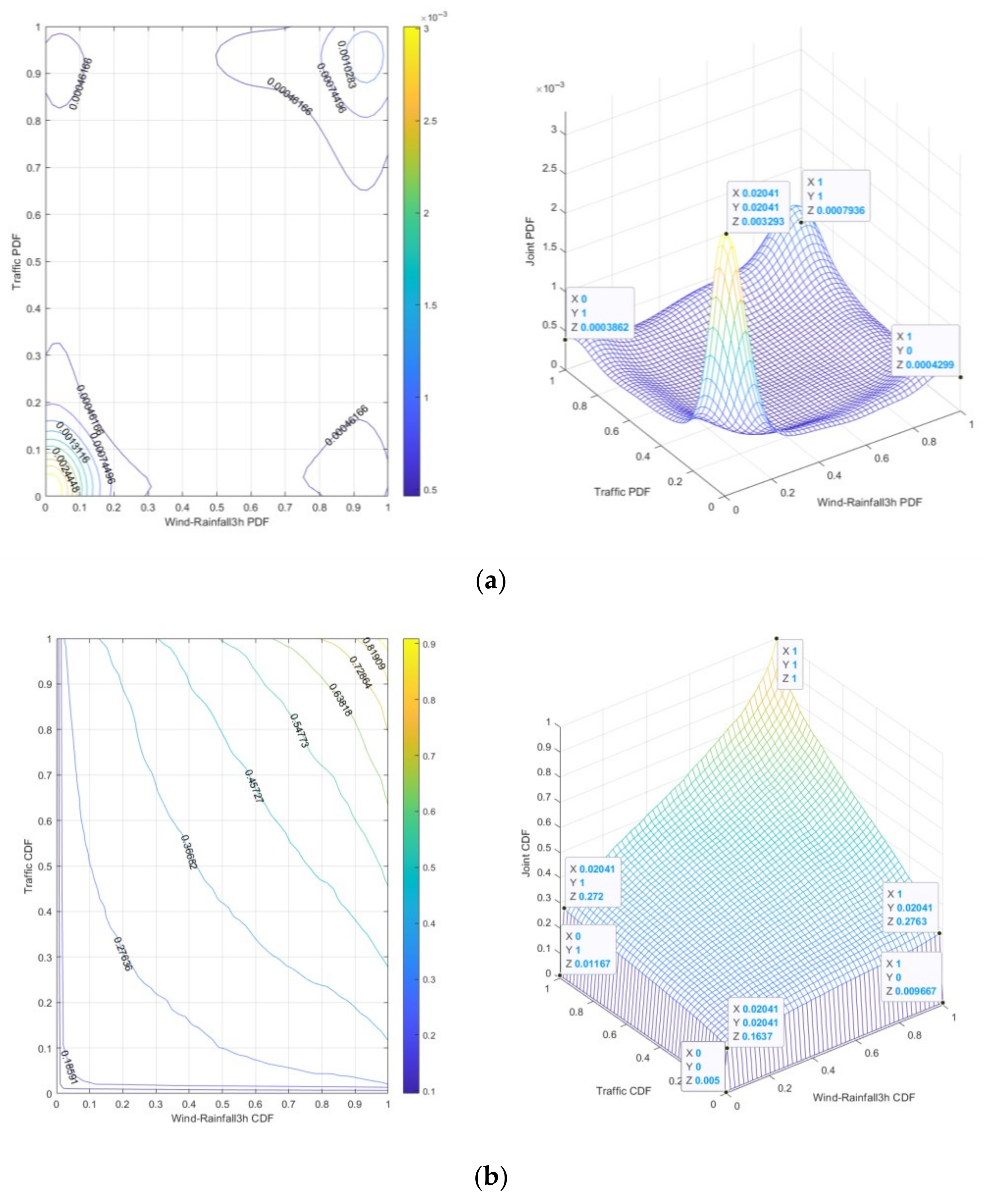
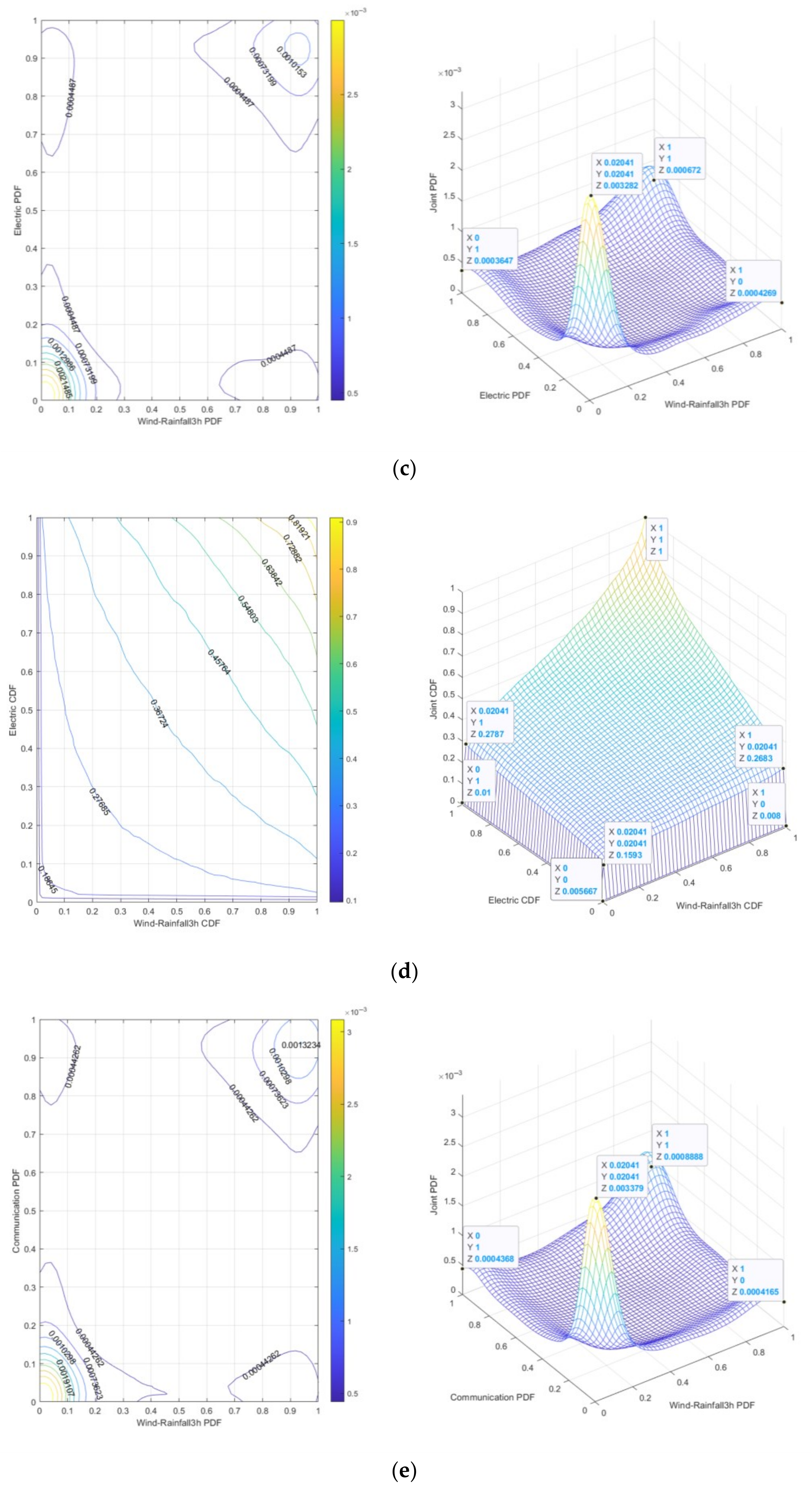
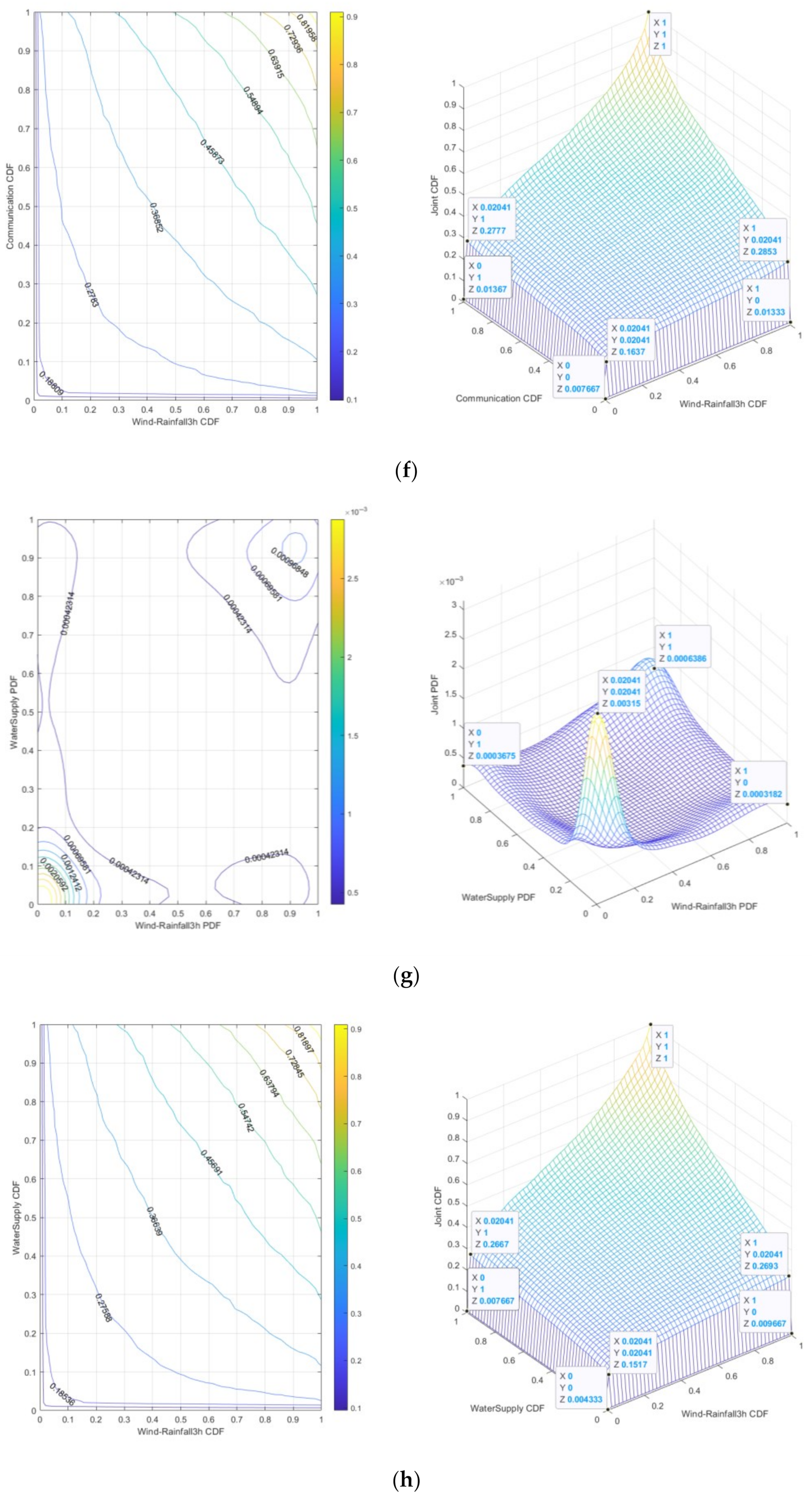
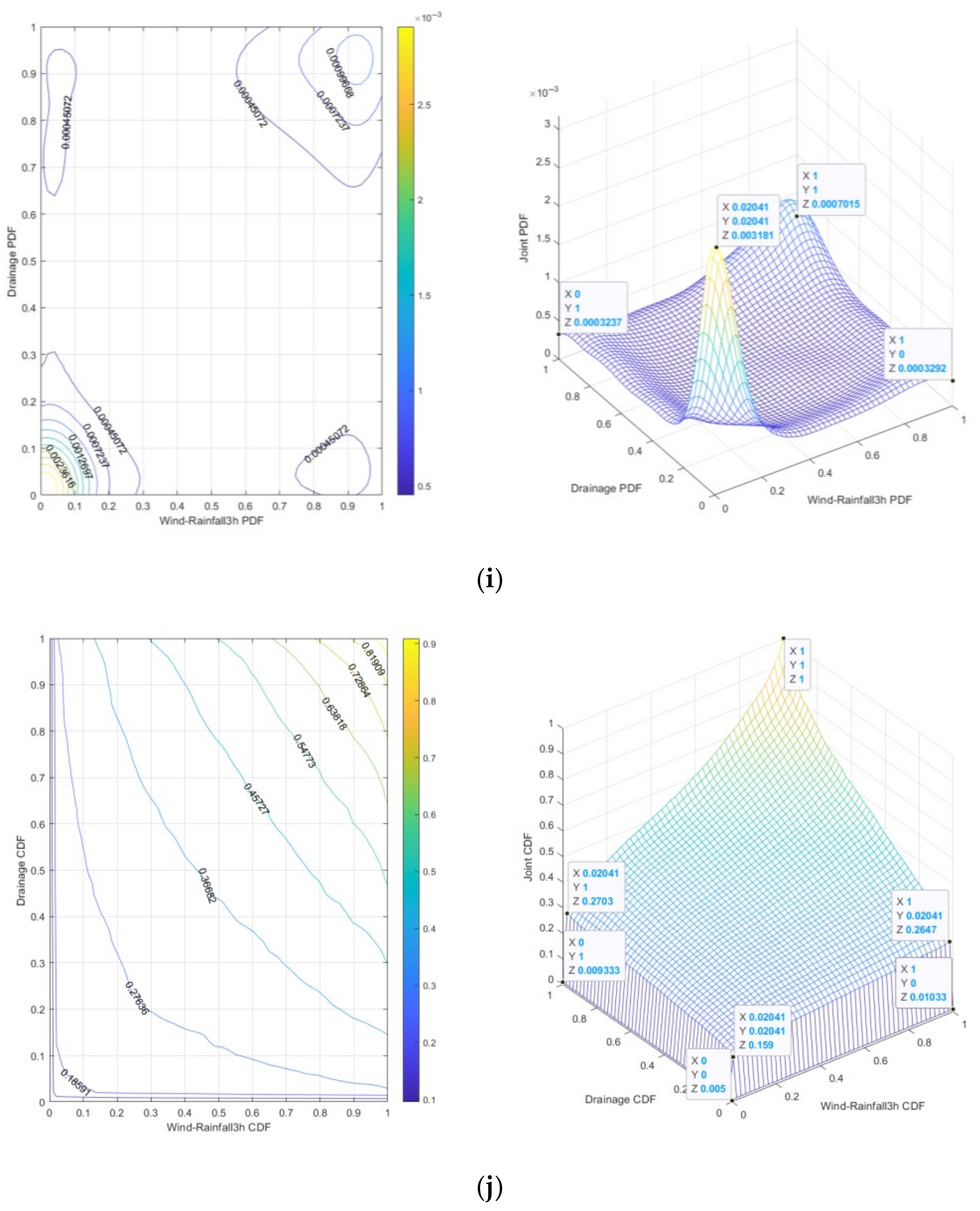
Based on the numerical simulation of joint probability density functions and joint cumulative probability functions for the risk evolution of 3 h Rainfall-Wind speed-Traffic/Electric/Communication/Water supply/Drainage systems using the Gumbel Copula function, as shown in Figure 7, by analyzing Figure 7 in conjunction with Figure 3, Figure 4 and Figure 6, it is determined that when the 3 h Rainfall is 341.9 mm and the Wind speed is 4.499 m/s:
(1)
The 3 h Rainfall-Wind speed-Traffic risk is “dark red”. It can be seen from Figure 7a that the peak joint probability density is 0.003293, indicating that under specific 3 h Rainfall-Wind speed and Traffic risk conditions, the probability of 3 h Rainfall-Wind speed-Traffic risk is relatively high. It can be seen from Figure 7b that the joint cumulative probability range is 0.005~0.1637, which means that under low-risk conditions, a small change of 3 h Rainfall-Wind speed-Traffic risk may lead to a significant increase in risk.
(2)
The 3 h Rainfall-Wind speed-Electric risk is “dark red”. It can be seen from Figure 7c that the peak value of joint probability density is 0.003282, indicating that under the specific conditions of 3 h Rainfall-Wind speed and Electric risk, the probability of 3 h Rainfall-Wind speed-Electric risk is relatively high. It can be seen from Figure 7d that the joint cumulative probability range is 0.005667~0.1593, which means that under low-risk conditions, a small change in 3 h Rainfall-Wind speed-Electric risk may lead to a significant increase in risk.
(3)
The 3 h Rainfall-Wind speed-Communication risk is “dark red”. It can be seen from Figure 7e that the peak value of joint probability density is 0.003379, indicating that under specific 3 h Rainfall-Wind speed and Communication conditions, the probability of 3 h Rainfall-Wind speed-Communication risk is relatively high. It can be seen from Figure 7f that the joint cumulative probability range is 0.007667~0.1637, which means that under low-risk conditions, a small change in 3 h Rainfall-Wind speed-Communication risk may lead to a significant increase in risk.
(4)
The 3 h Rainfall-Wind speed-Water supply risk is “dark red”. It can be seen from Figure 7g that the peak value of joint probability density is 0.00315, which indicates that under specific 3 h Rainfall-Wind speed and Water supply conditions, the probability of 3 h Rainfall-Wind speed-Water supply risk is relatively high. It can be seen from Figure 7h that the joint cumulative probability range is 0.004333~0.1517, which means that under low-risk conditions, a small change in 3 h Rainfall-Wind speed-Water supply risk may lead to a significant increase in risk.
(5)
The 3 h Rainfall-Wind speed-Drainage risk is “red”. It can be seen from Figure 7i that the peak value of joint probability density is 0.003181, which indicates that under specific conditions of 3 h Rainfall-Wind speed and Drainage, the probability of 3 h Rainfall-Wind speed-Drainage risk is relatively high. It can be seen from Figure 7j that the joint cumulative probability range is 0.005~0.159, which means that under low-risk conditions, a small change in 3 h Rainfall-Wind speed-Drainage risk may lead to a significant increase in risk.
Based on Figure 7, it can be seen from the dense distribution of contour lines and the three-dimensional significant single peak characteristics that the joint occurrence of 3 h Rainfall-Wind speed-Traffic/Electric/Communication/Water supply/Drainage (1st-order) risk has a high concentration and high probability density in the low-risk range. As the risk range increases (high-risk range), the probability density significantly decreases and the contour lines become sparse, reflecting a lower probability of joint occurrence of risk factors under extreme conditions. The cumulative probability gradient of the low-risk range is steep, which indicates that in a short time, a small fluctuation of 1st-order risk can trigger the crossing of the risk threshold. The cumulative probability gradient of the low-risk value domain is steep, which means that in a short time, the small fluctuation of 1st-order risk can trigger the crossing of the risk threshold. In the high-value range, the cumulative probability gradient slows down, indicating that the risk accumulation tends to saturate. Under different risk combinations of 1st-order, the cumulative probability varies widely, reflecting the dynamic evolution characteristics of risk. The strong tail correlation of 1st-order low-risk range dominates the risk coupling effect, while the independence of high-risk range variables is enhanced.
From the perspective of urban lifeline Natech event risk management, the peak values of joint probability density for risk evolution characterize the propagation velocity of risks across Traffic, Electric, Communication, Water supply, and Drainage systems under 3 h Rainfall-Wind speed scenarios. Higher peaks indicate shorter “Golden Response Windows” available to urban lifeline management departments and emergency agencies. Similarly, the range of joint cumulative probability for risk evolution defines the buffer zone capacity within these infrastructure networks during 3 h Rainfall-Wind speed scenarios. Narrower ranges signify that even minor perturbations could plunge urban lifelines directly into extreme operational states.
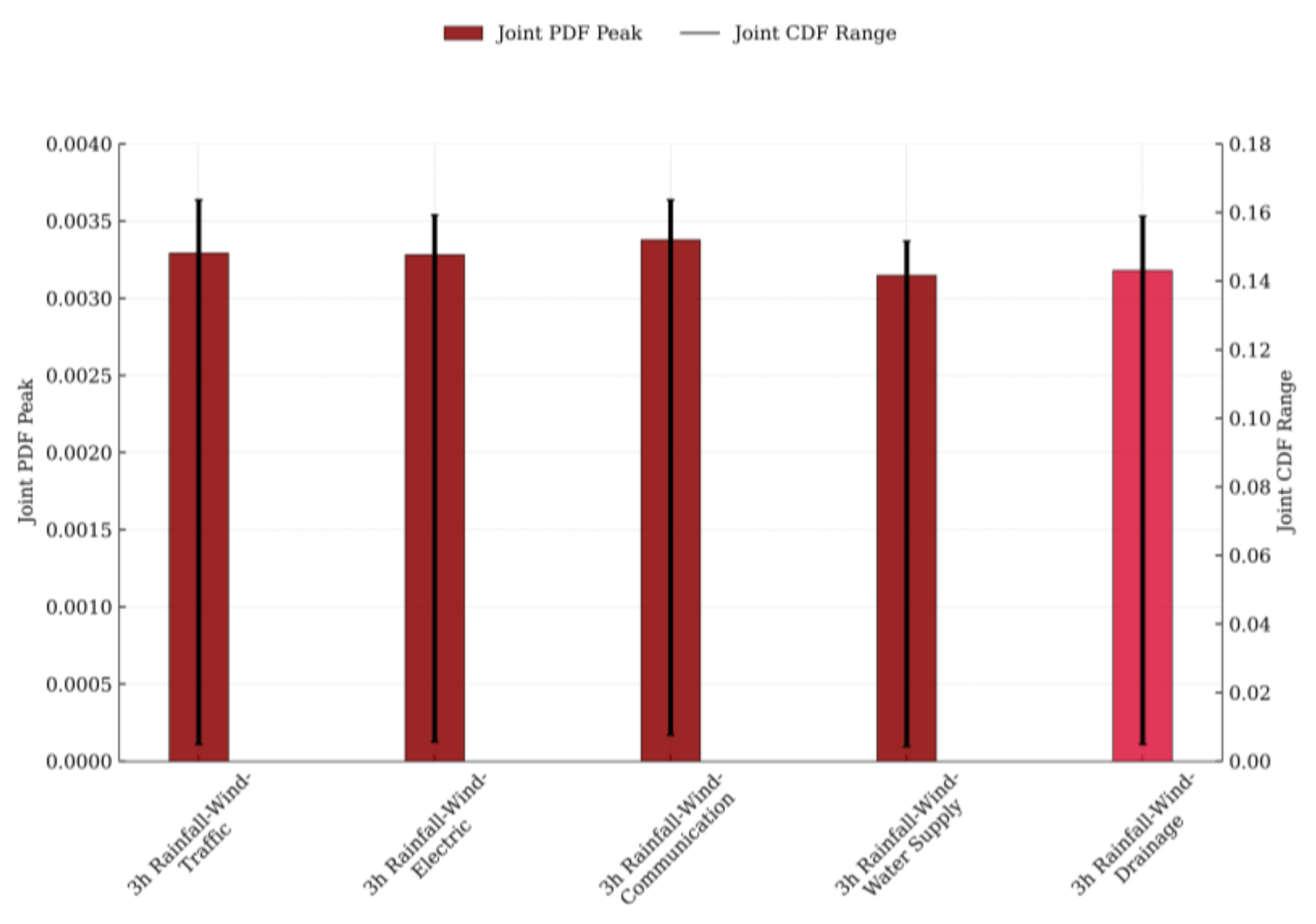
The peak ranks of joint probability density for 1st-order risk evolution in urban lifeline Natech events are as follows: 3 h Rainfall-Wind speed-Communication, 3 h Rainfall-Wind speed-Traffic, 3 h Rainfall-Wind speed-Electric, 3 h Rainfall-Wind speed-Drainage, and 3 h Rainfall-Wind speed-Water supply. The scope ranks of joint cumulative probability for 1st-order risk evolution follow this sequence: 3 h Rainfall-Wind speed-Communication, 3 h Rainfall-Wind speed-Drainage, 3 h Rainfall-Wind speed-Water supply, 3 h Rainfall-Wind speed-Traffic, and 3 h Rainfall-Wind speed-Electric. Figure 8 illustrates both the peak joint probability density and the range of joint cumulative probability for these 1st-order risks.
The traffic system is a dynamic network influenced by multiple variables (e.g., vehicle density, road conditions, traffic signals). Rainstorms reduce visibility and cause vehicle skidding, while gales damage signage and fell trees block routes. Risk propagates rapidly under storm conditions—localized accidents or congestion quickly cascade to surrounding areas. Its geographically dispersed infrastructure and diverse participants (pedestrians, cyclists, motorists) amplify impact zones. The electric system comprises transmission lines, substations, and critical facilities. Rainstorms trigger utility pole collapses and substation flooding, gales induce line breaks and short circuits. Risk spreads moderately due to robust protective measures (wind/rain resistance designs). However, system stability heavily depends on equipment integrity—partial outages can destabilize entire networks. The communication system includes base stations and communication lines. Rainstorm and gale impacts manifest as flooded base stations and severed cables. Risk propagates the fastest: single-station failure often cripples adjacent nodes via backhaul interruption. Despite inherent resilience (waterproof designs, reinforced lines, redundant architectures across modes/routes), its localized disruptions remain minimal. The drainage system is primarily designed for stormwater/wastewater discharge. Rainstorms overwhelm capacity, causing urban flooding; gales block grates with debris, worsening efficiency. Risk spreads slowly—rain dominates pressure, while wind contributes marginally. Purpose-built redundancy concentrates impact zones, though cumulative effects accelerate failure progression. The water supply system consists of sources, pipelines, and treatment plants. Rainstorms introduce contaminants (silt, trash); gales carry dust into facilities/pipes. The lowest risk propagation rate is owed to storage/regulation capabilities, physical redundancy (plants, pumps, pipes), and manual switching options. While damages are typically localized, recovery is complex and prolonged.
Traffic, electric, and communication systems—characterized by their widespread facility distribution and high environmental sensitivity—exhibit elevated probabilities of 1st-order technical accidents and greater potential for cumulative risk escalation under specific rainstorm and gale scenarios. In contrast, while Water supply and Drainage systems are also impacted by such weather extremes, their relatively centralized layout, protective safeguards, and slower risk propagation dynamics mitigate these effects.

5.2.2. Joint Probability Distribution of 3 h Rainfall-Wind Speed-Urban Lifelines 2nd-Order Risk Evolution

Under rainstorm and gale scenarios, the propagation of technical accident risks within urban lifeline systems demonstrates a domino effect—wherein risks diffuse and accumulate across the buffer zones of interconnected systems, driving the evolution of 1st-order technical accidents into 2nd-order risks. Based on the numerical simulation of joint probability density functions and joint cumulative probability functions, we used the Gumbel Copula function for the 2nd-order risk evolution of the following coupled systems: 3 h Rainfall-Wind speed-Drainage-Traffic, 3 h Rainfall-Wind speed-Drainage-Electric, 3 h Rainfall-Wind speed-Drainage-Communication, 3 h Rainfall-Wind speed-Drainage-Water supply, 3 h Rainfall-Wind speed-Water supply-Traffic, 3 h Rainfall-Wind speed-Electric-Water supply, 3 h Rainfall-Wind speed-Communication-Traffic, and 3 h Rainfall-Wind speed-Electric-Communication, as shown in Figure 9. By analyzing Figure 9 in conjunction with Figure 3, Figure 4 and Figure 6, it is determined that when the 3 h Rainfall is 341.9 mm and the Wind speed is 4.499 m/s:
(1)
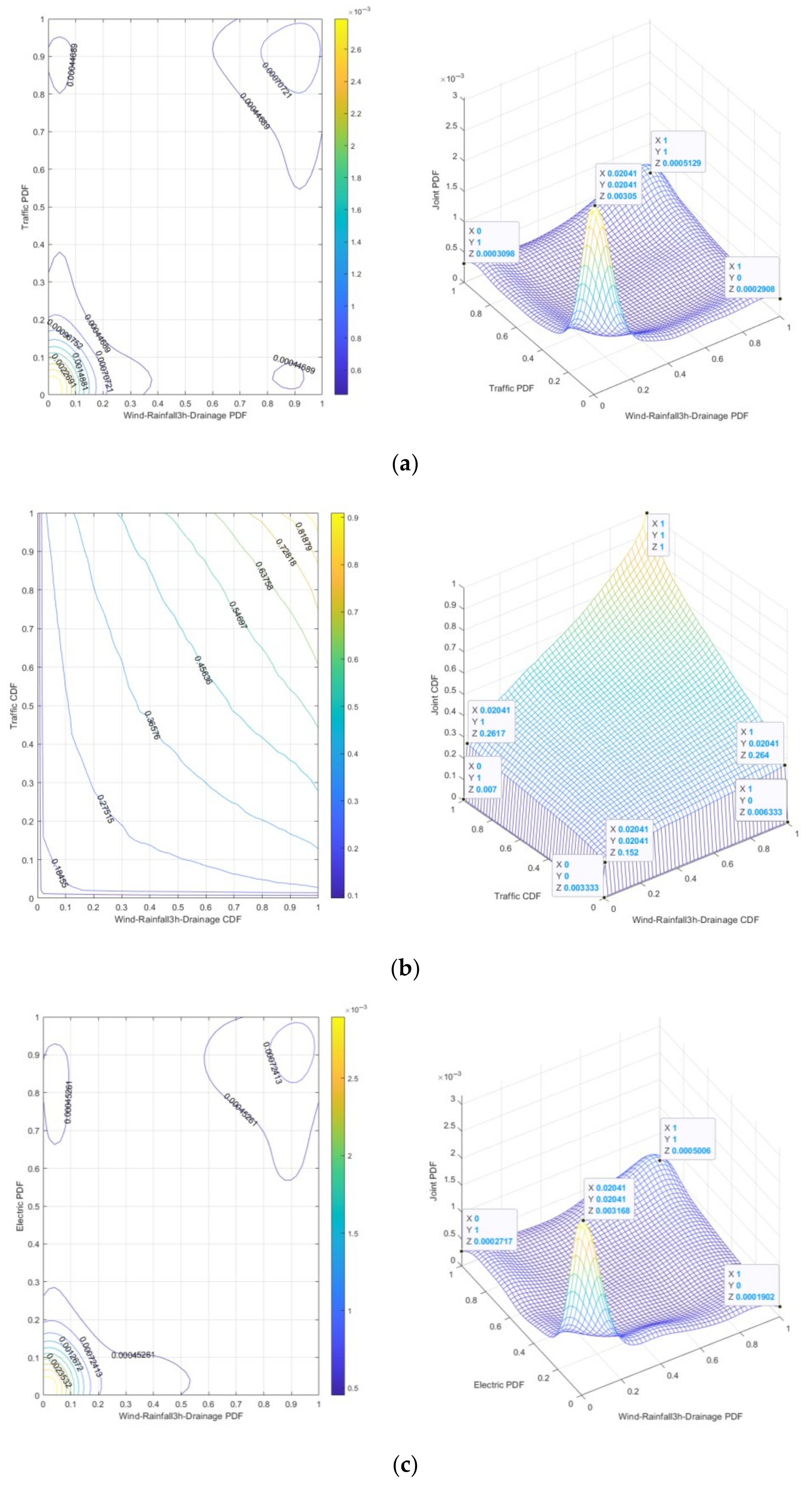
The 3 h Rainfall-Wind speed-Drainage-Traffic risk is “dark red”. It can be seen from Figure 9a that the peak value of joint probability density is 0.00305, indicating that under specific 3 h Rainfall-Wind speed and Drainage-Traffic conditions, the probability of 3 h Rainfall-Wind speed-Drainage-Traffic risk is relatively high. It can be seen from Figure 9b that the joint cumulative probability range is 0.003333~0.152, which means that under low-risk conditions, small changes in 3 h Rainfall-Wind speed-Drainage-Traffic risk may lead to a significant increase in risk.
(2)
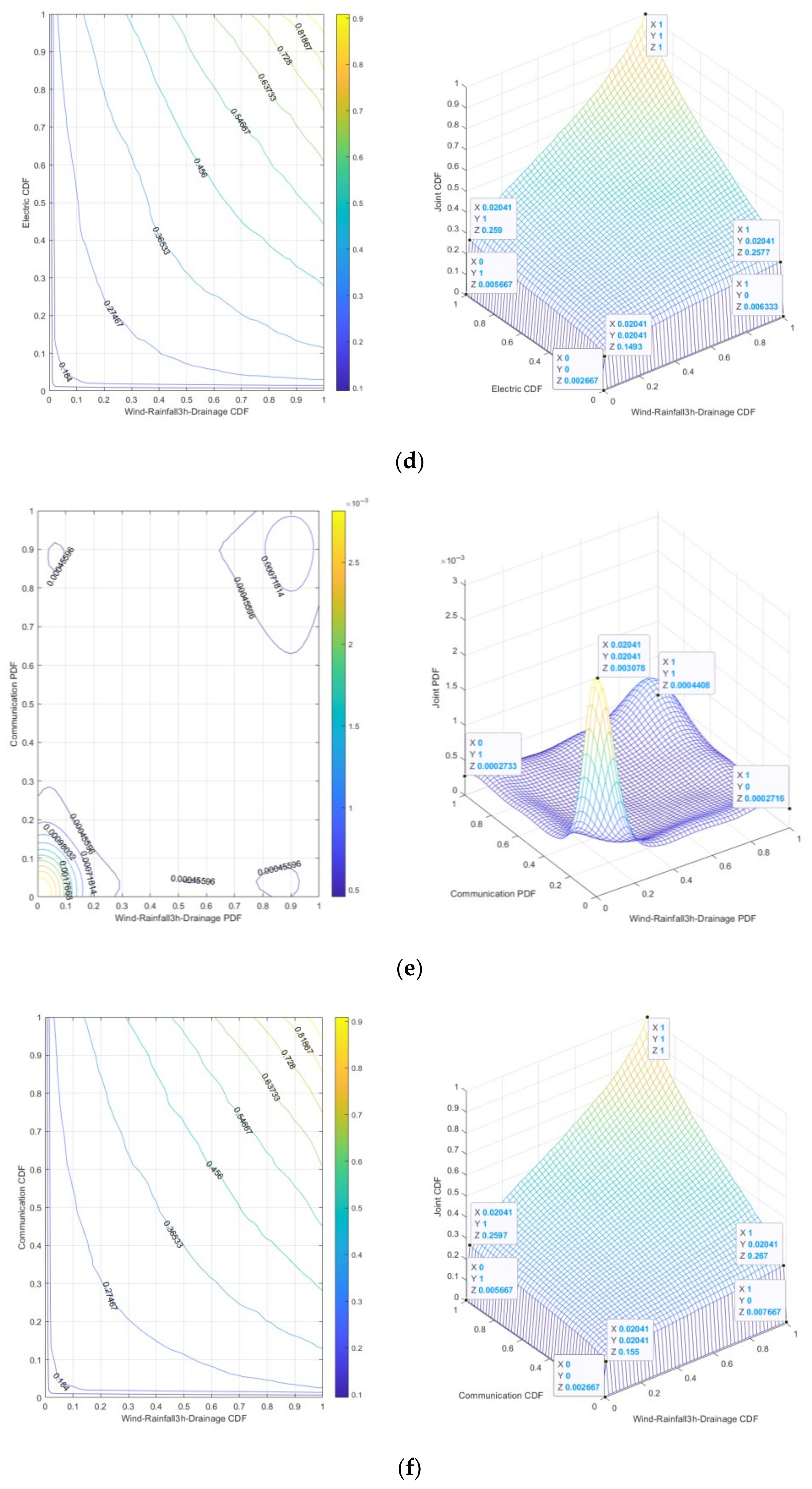
The 3 h Rainfall-Wind speed-Drainage-Electric risk is “dark red”. It can be seen from Figure 9c that the peak value of joint probability density is 0.003168, indicating that under the specific conditions of 3 h Rainfall-Wind speed and Drainage-Electric, the probability of 3 h Rainfall-Wind speed-Drainage-Electric risk is relatively high. It can be seen from Figure 9d that the joint cumulative probability range is 0.002667~0.1493, which means that under low-risk conditions, small changes in 3 h Rainfall-Wind speed-Drainage-Electric risk may lead to a significant increase in risk.
(3)
The 3 h Rainfall-Wind speed-Drainage-Communication risk is “dark red”. It can be seen from Figure 9e that the peak value of joint probability density is 0.003078, indicating that under specific conditions of 3 h Rainfall-Wind speed and Drainage-Communication, the probability of 3 h Rainfall-Wind speed-Drainage Communication risk is relatively high. It can be seen from Figure 9f that the joint cumulative probability range is 0.002667~0.155, which means that under low-risk conditions, small changes in 3 h Rainfall-Wind speed-Drainage-Communication risk may lead to significant increases in risks.
(4)
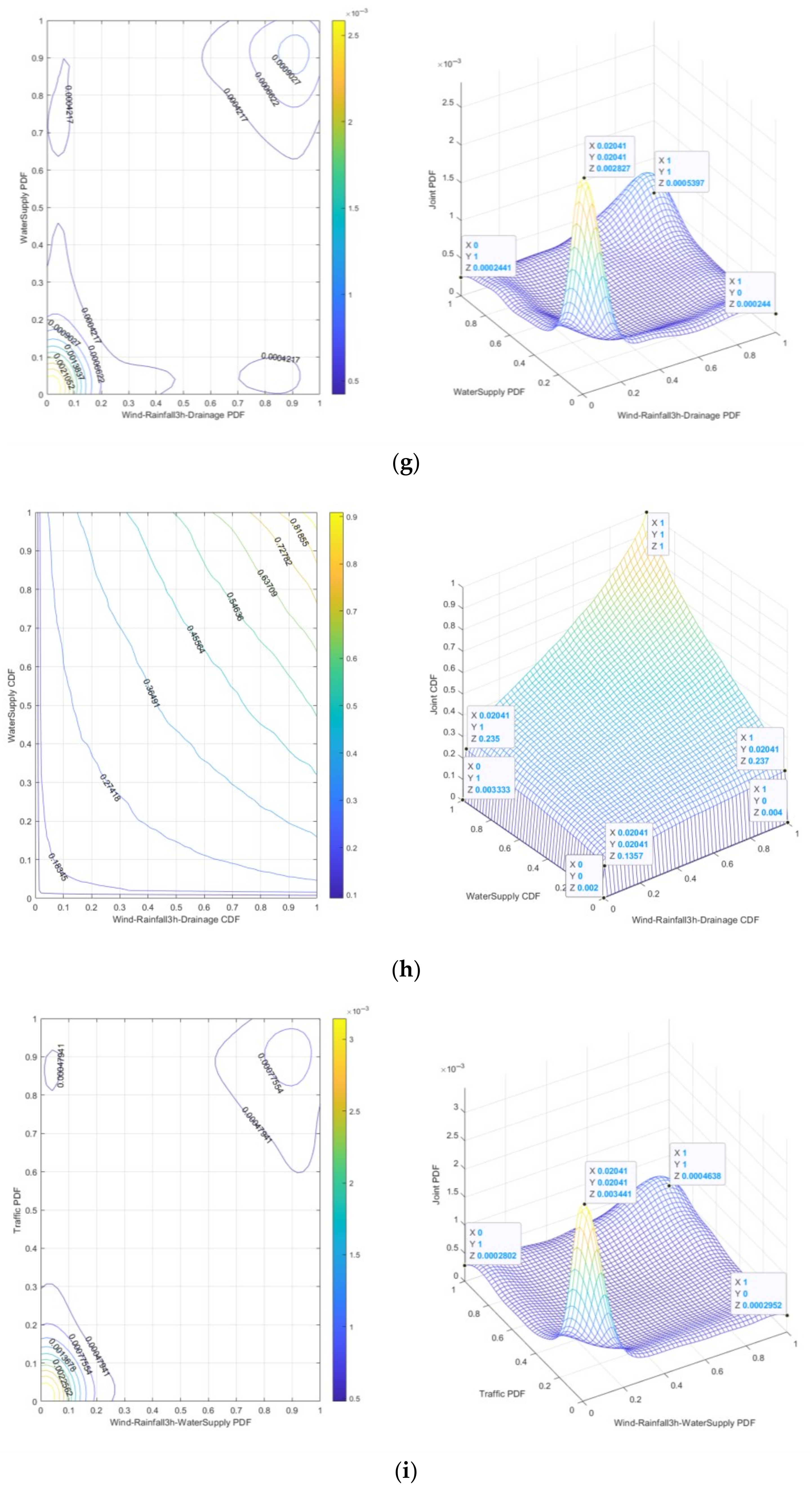
The 3 h Rainfall-Wind speed-Drainage-Water supply risk is “dark red”. It can be seen from Figure 9g that the peak value of joint probability density is 0.002827, which indicates that under specific conditions of 3 h Rainfall-Wind speed and Drainage-Water supply, the probability of 3 h Rainfall-Wind speed-Drainage-Water supply risk is relatively high. It can be seen from Figure 9h that the joint cumulative probability range is 0.002~0.1357, which means that under low-risk conditions, a small change of 3 h Rainfall-Wind speed-Drainage-Water supply risk may lead to a significant increase in risk.
(5)
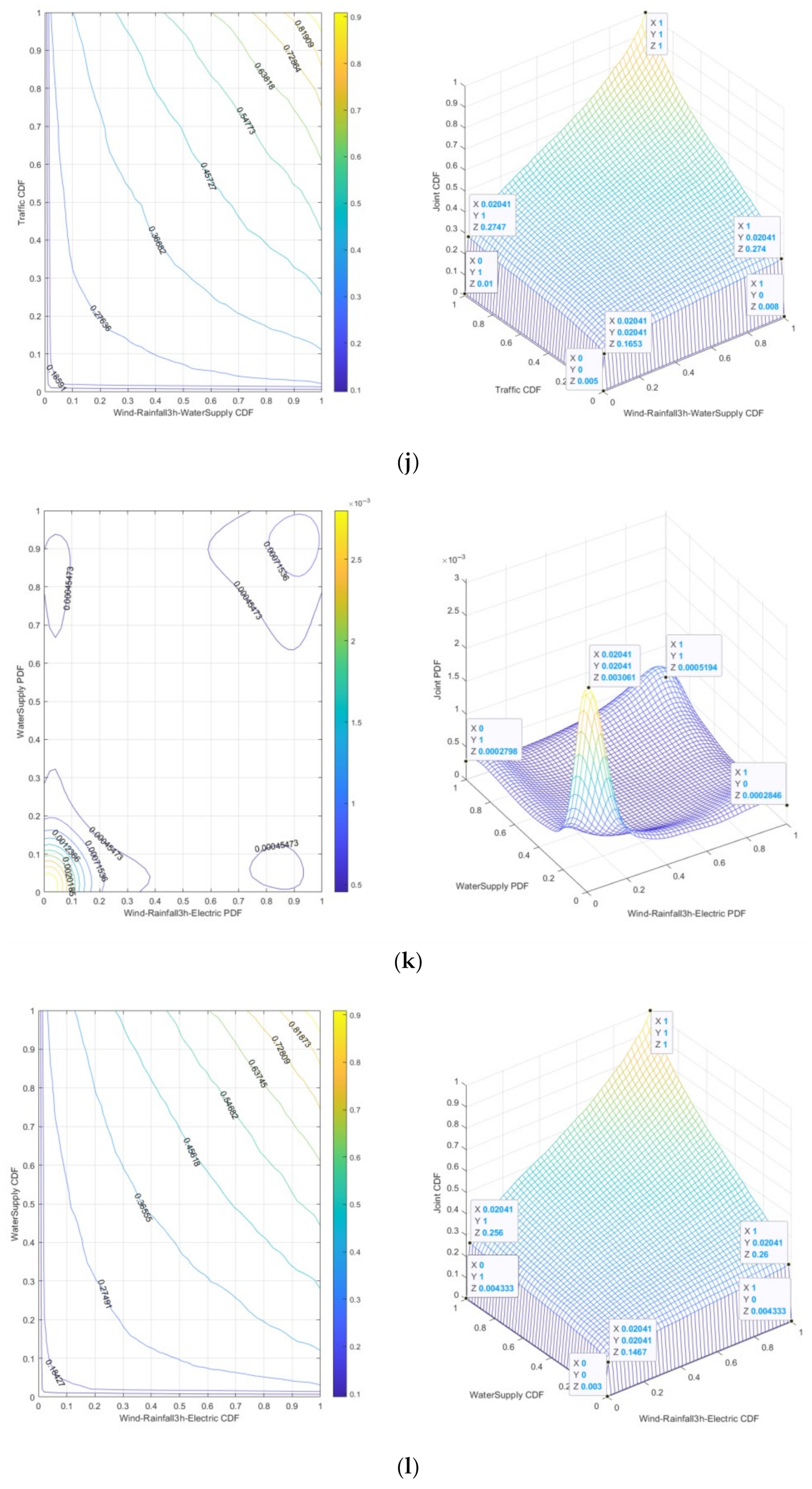
The 3 h Rainfall-Wind speed-Water supply-Traffic risk is “dark red”. It can be seen from Figure 9i that the peak value of joint probability density is 0.003441, which indicates that under the specific conditions of 3 h Rainfall-Wind speed and Water supply-Traffic, the probability of 3 h Rainfall-Wind speed-Water supply-Traffic risk is relatively high. It can be seen from Figure 9j that the joint cumulative probability range is 0.005~0.1653, which means that under low-risk conditions, small changes in 3 h Rainfall-Wind speed-Water supply-Traffic risk may lead to significant increases in risks.
(6)
The 3 h Rainfall-Wind speed-Electric-Water supply risk is “dark red”. It can be seen from Figure 9k that the peak value of joint probability density is 0.003061, which indicates that under specific conditions of 3 h Rainfall-Wind speed and Electric-Water supply, the probability of 3 h Rainfall-Wind speed-Electric-Water supply risk is relatively high. It can be seen from Figure 9l that the joint cumulative probability range is 0.003~0.1467, which means that under low-risk conditions, a small change in 3 h Rainfall-Wind speed-Electric-Water supply risk may lead to a significant increase in risk.
(7)
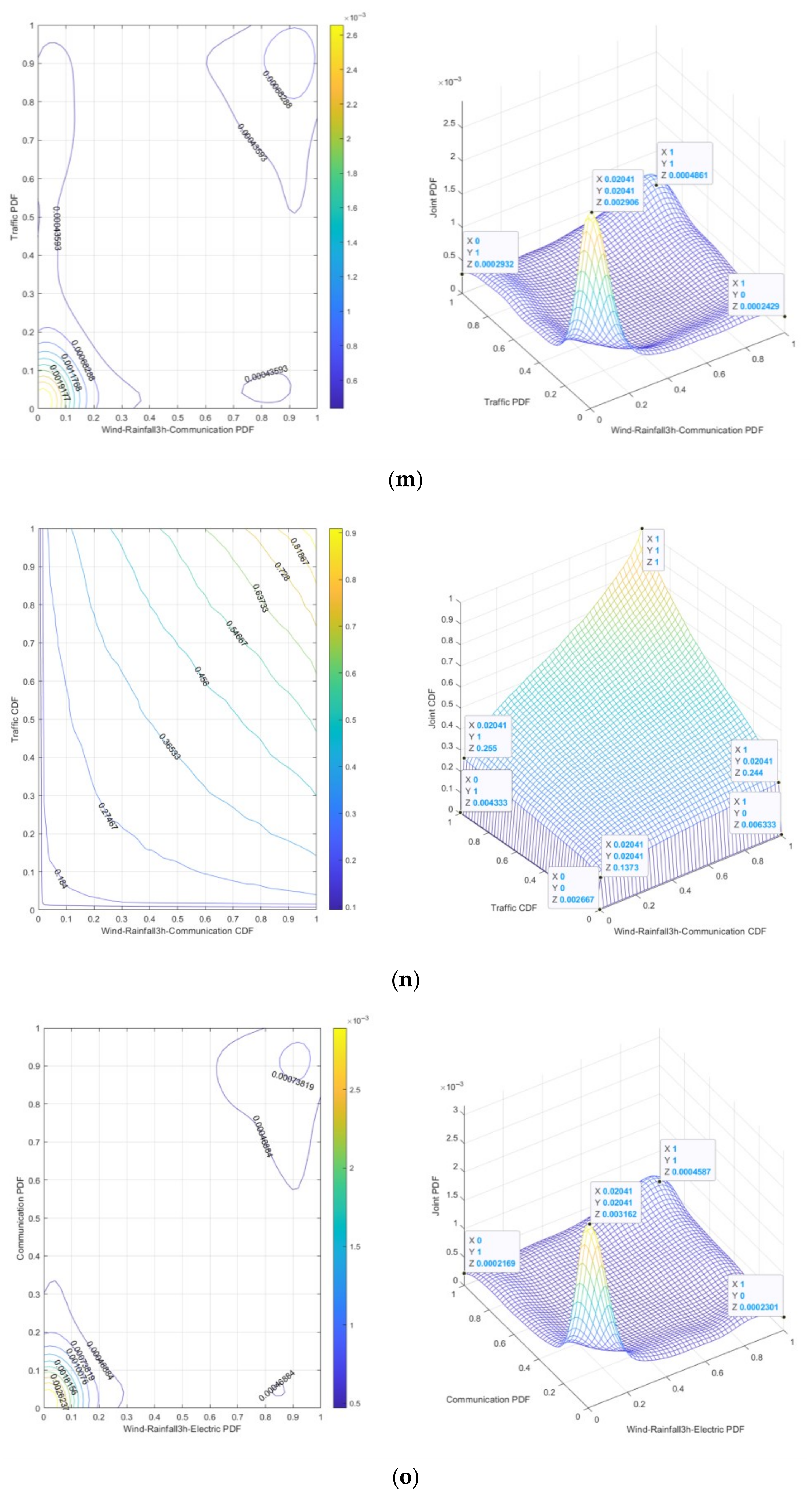
The 3 h Rainfall-Wind speed-Communication-Traffic risk is “dark red”. It can be seen from Figure 9m that the peak value of joint probability density is 0.002906, indicating that under the specific conditions of 3 h Rainfall-Wind speed and Communication-Traffic, the probability of 3 h Rainfall-Wind speed-Communication-Traffic risk is relatively high. It can be seen from Figure 9n that the joint cumulative probability range is 0.002667~0.1373, which means that under low-risk conditions, a small change in 3 h Rainfall-Wind speed-Communication-Traffic risk may lead to a significant increase in risk.
(8)
The 3 h Rainfall-Wind speed-Electric-Communication risk is “dark red”. It can be seen from Figure 9k that the peak value of joint probability density is 0.003162, which indicates that under specific conditions of 3 h Rainfall-Wind speed and Electric-Communication, the probability of 3 h Rainfall-Wind speed-Electric-Communication risk is relatively high. It can be seen from Figure 9l that the joint cumulative probability range is 0.002~0.1587, which means that under low-risk conditions, a small change in 3 h Rainfall-Wind speed-Electric-Communication risk may lead to a significant increase in risk.
Based on Figure 9, it can be seen from the dense distribution of contour lines and the three-dimensional significant single peak characteristics that the strong tail correlation dominates the risk coupling effect in the low-risk range. The joint occurrence of 3 h Rainfall-Wind speed risk and Drainage-Traffic/Drainage-Electric/Drainage-Communication/Drainage-Water supply/Water supply-Traffic/Electric-Water supply/Communication-Traffic/Electric-Communication (2nd-order) risk has a high concentration and high probability density. With the increase in risk value range (high risk value range), the independence of 2nd-order risk increases, the probability density decreases significantly, and the contour becomes sparse, reflecting the low probability of the joint occurrence of risk factors under extreme conditions. The cumulative probability gradient is steep, indicating that in a short time, a small fluctuation of 2nd-order risk can trigger the crossing of the risk threshold. The gradient of cumulative probability is slowing down, indicating that the accumulation of risk is approaching saturation.
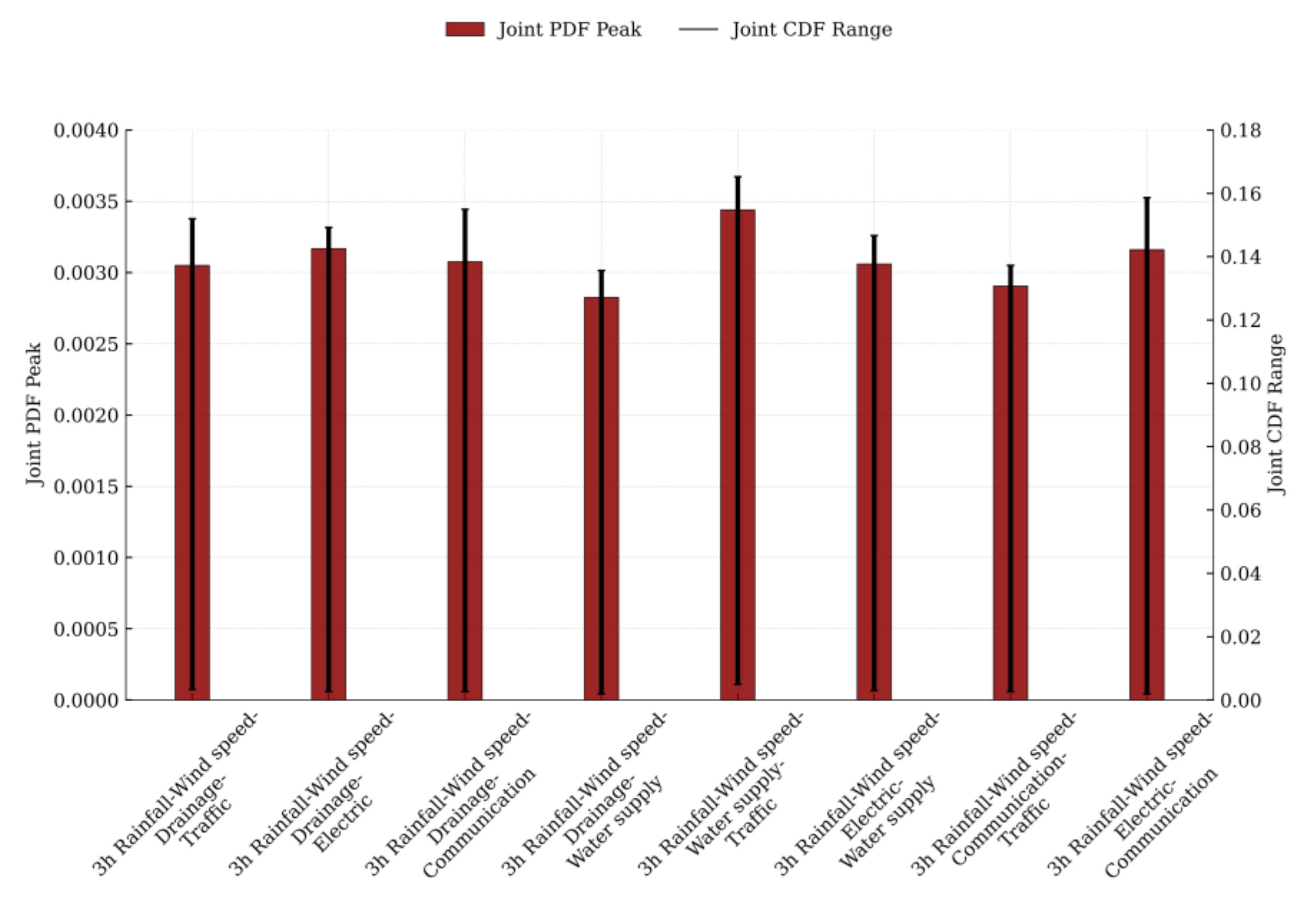
The peak ranks of joint probability density for 2nd-order risk evolution in urban lifeline Natech events are as follows: 3 h Rainfall-Wind speed-Water supply-Traffic, 3 h Rainfall-Wind speed-Drainage-Electric, 3 h Rainfall-Wind speed-Electric-Communication, 3 h Rainfall-Wind speed-Drainage-Communication, 3 h Rainfall-Wind speed-Electric-Water supply, 3 h Rainfall-Wind speed-Drainage-Traffic, 3 h Rainfall-Wind speed-Communication-Traffic, and 3 h Rainfall-Wind speed-Drainage-Water supply. The scope ranks of joint cumulative probability for 2nd-order risk evolution in urban lifeline Natech events are as follows: 3 h Rainfall-Wind speed-Water supply-Traffic, 3 h Rainfall-Wind speed-Electric-Communication, 3 h Rainfall-Wind speed-Drainage-Communications, 3 h Rainfall-Wind speed-Drainage–Traffic, 3 h Rainfall-Wind speed-Drainage-Electric, 3 h Rainfall-Wind speed-Electric-Water supply, 3 h Rainfall-Wind speed-Communication-Traffic, and 3 h Rainfall-Wind speed-Drainage-Water supply. Figure 10 illustrates both the peak joint probability density and the range of joint cumulative probability for these 2nd-order risks.
Under 3 h Rainfall-Wind speed scenarios:
Water supply-Traffic 2nd-order risk exhibits the fastest propagation speed. Nevertheless, the Traffic network’s structural resilience and the Water supply system’s redundant design preserve the largest buffer zone, manifesting as “Rapid Escalation but Effective Containment”. Drainage-Electric 2nd-order risk propagates quickly, yet the Electric system’s redundancy partially offsets Drainage vulnerabilities, maintaining a moderate buffer zone characterized by “Swift Progression with Limited Maneuverability”. Electric-Communication 2nd-order risk features rapid chain-reaction potential. However, the Communications system’s redundancy neutralizes most Electric-related risks, sustaining a substantial buffer zone described as “Cascading Failure Prone but Abundant Backup Pathways Available”. Drainage-Communication 2nd-order risk demonstrates relatively fast propagation. The Communication system’s redundancy mitigates significant Drainage risks, retaining a sizable buffer zone evident in “Flooding Accelerates, yet Communication Endures”. Electric-Water supply 2nd-order risk slowest-propagating among pairs. Minimal compensation occurs via Water supply redundancy against Electric risks, resulting in a small buffer zone reflected in “Gradual Degradation with Constrained Mitigation Options”. Drainage-Traffic 2nd-order risk moderate propagation speed. The Traffic network’s structural advantages largely counteract Drainage impacts, preserving a notable buffer zone summarized as “Pooling Rapidly but Detournable”. Communication-Traffic 2nd-order risk has the slowest propagation overall. Lacking sufficient compensatory mechanisms from the Traffic network, this pair maintains a minimal buffer zone, embodying “Sluggish yet Fragile”. Drainage-Water supply 2nd-order risk is the slowest-moving risk sequence. Water supply redundancy fails to adequately address Drainage vulnerabilities, yielding the smallest buffer zone characterized by “Persistent Erosion with Minimal Cushioning”.

5.2.3. Joint Probability Distribution of 3 h Rainfall-Wind Speed-Urban Lifelines 3rd-Order to 5th-Order Risk Evolution

Under 3 h Rainfall-Wind speed scenarios, the propagation of technical accident risks within urban lifeline systems exhibits a domino effect—wherein risks spread and accumulate across the buffer zones of interconnected systems, driving the evolution of 2nd-order technical accidents into 3rd-order to 5th-order technical accidents. Based on the 3rd-order risk evolution of 3 h Rainfall-Wind speed-Drainage-Traffic-Electric, the 4th-order risk evolution of 3 h Rainfall-Wind speed-Drainage-Traffic-Electric-Communication, the 5th-order risk evolution of 3 h Rainfall-Wind speed-Drainage-Traffic-Electric-Communication-Water supply, numerical simulations of the joint probability distribution using the Gumbel Copula function were conducted. The joint probability density functions and joint cumulative probability functions are shown in Figure 11, Figure 12, and Figure 13, respectively. By combining Figure 3, Figure 4 and Figure 6, the analysis of Figure 11, Figure 12 and Figure 13 reveals the following under conditions of 3 h Rainfall of 341.9 mm and Wind speed of 4.499 m/s:
(1)
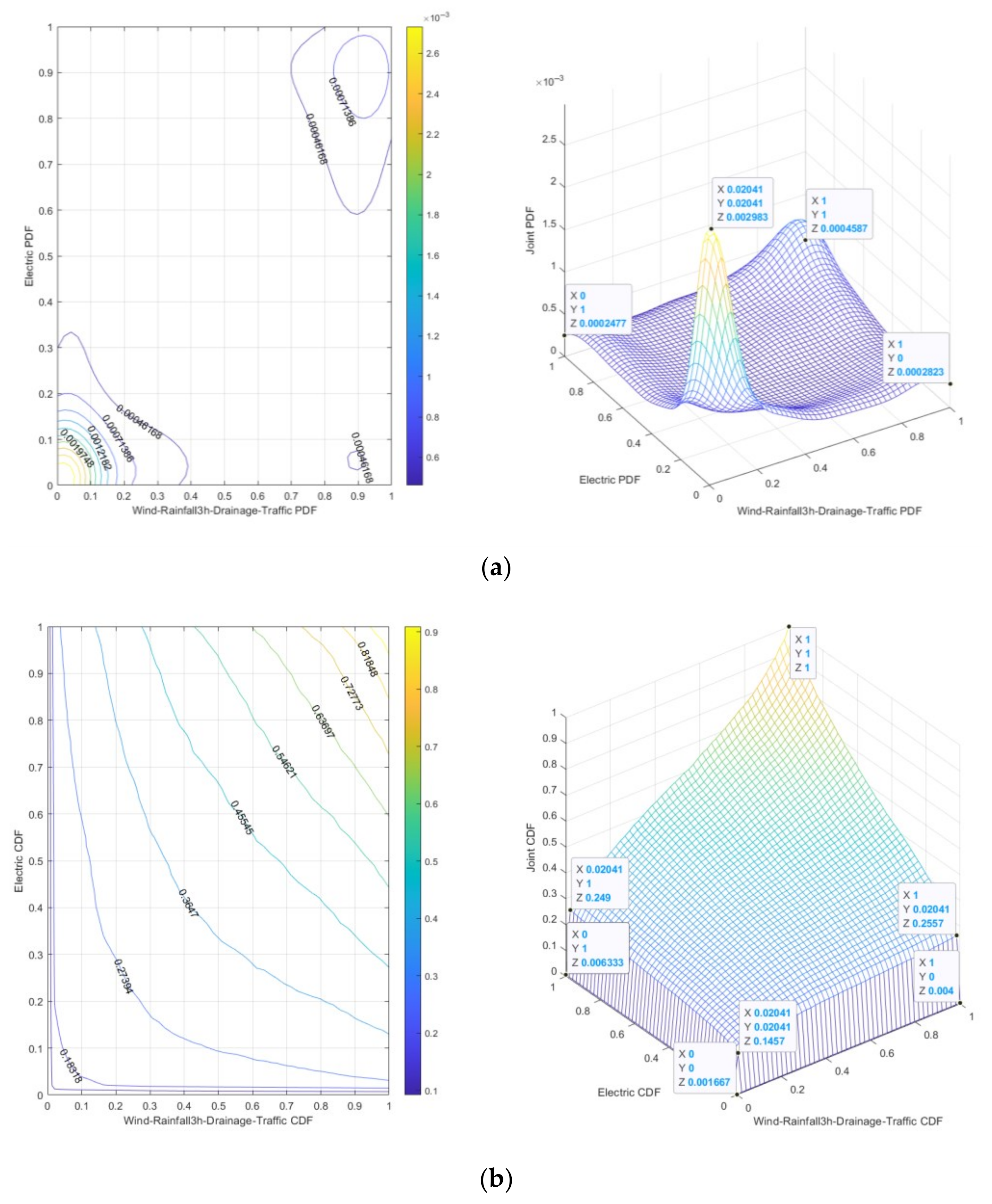
The 3 h Rainfall-Wind speed-Drainage-Traffic-Electric risk is “dark red”, indicating that under specific conditions of 3 h Rainfall-Wind speed and Drainage-Traffic-Electric, the probability of 3 h Rainfall-Wind speed-Drainage-Traffic-Electric risk is relatively high. It can be seen from Figure 11a that the peak value of joint probability density is 0.002983, and from Figure 11b that the range of joint cumulative probability is 0.001667~0.1457, which means that under low-risk conditions, a small change in 3 h Rainfall-Wind speed-Drainage-Traffic-Electric risk may lead to a significant increase in risk.
(2)
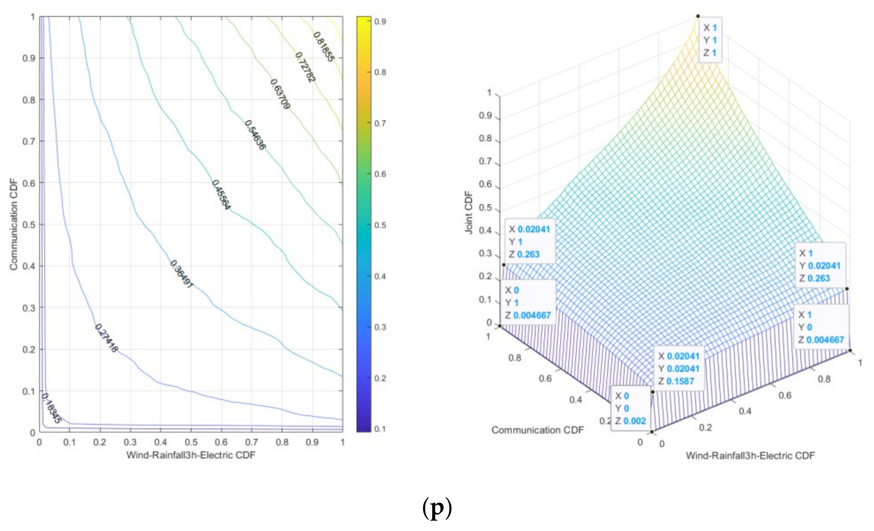
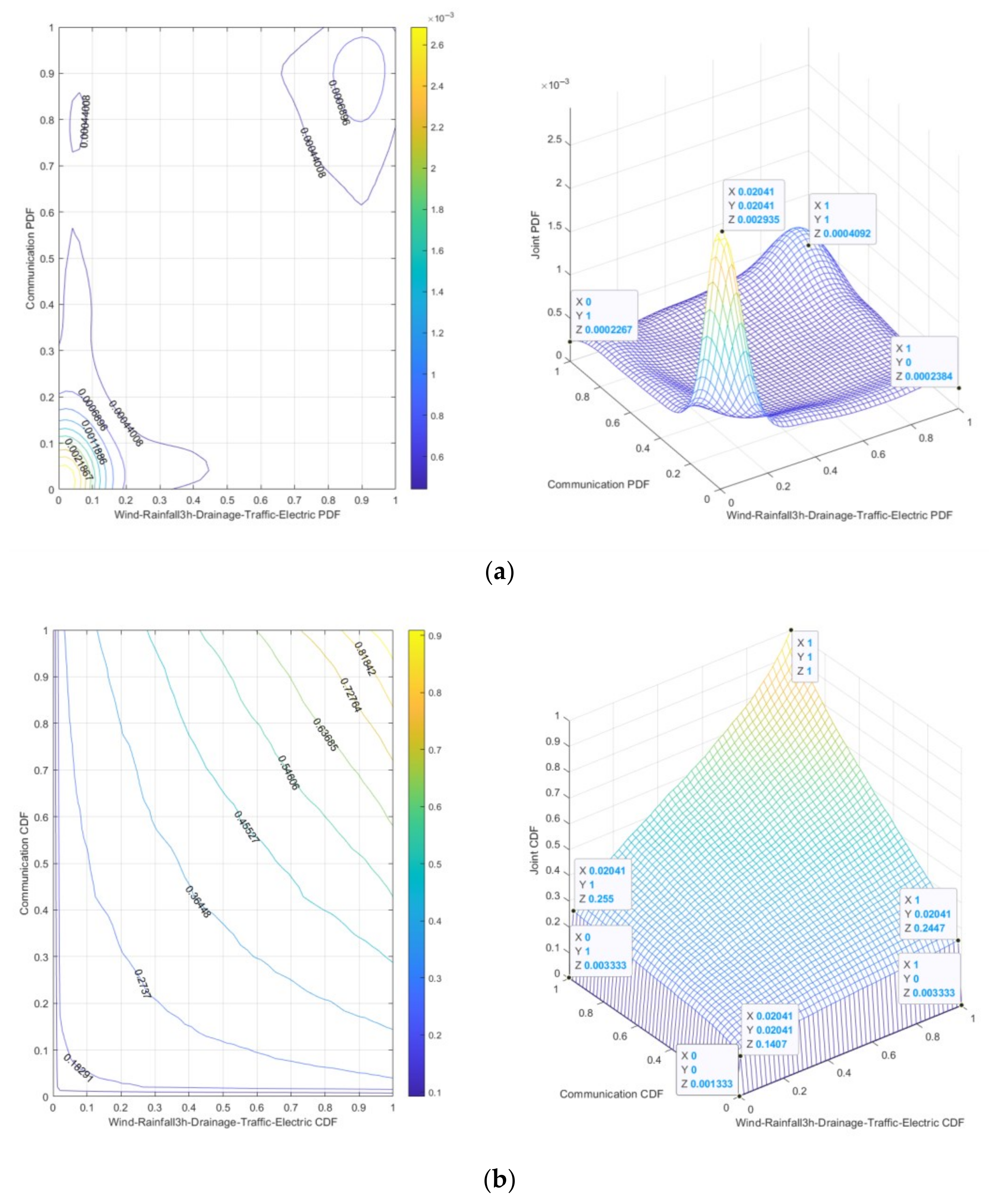
The 3 h Rainfall-Wind speed-Drainage-Traffic-Electric-Communication risk is “dark red”, indicating that under specific conditions of 3 h Rainfall-Wind speed and Drainage-Traffic-Electric-Communication, the probability of 3 h Rainfall-Wind speed-Drainage-Traffic-Electric-Communication risk is relatively high. It can be seen from Figure 12a that the peak joint probability density is 0.002935, and from Figure 12b that the joint cumulative probability range is 0.001333~0.1407, which means that under low-risk conditions, small changes in 3 h Rainfall-Wind speed-Drainage-Traffic-Electric-Communication risk may lead to significant increases in risks.
(3)
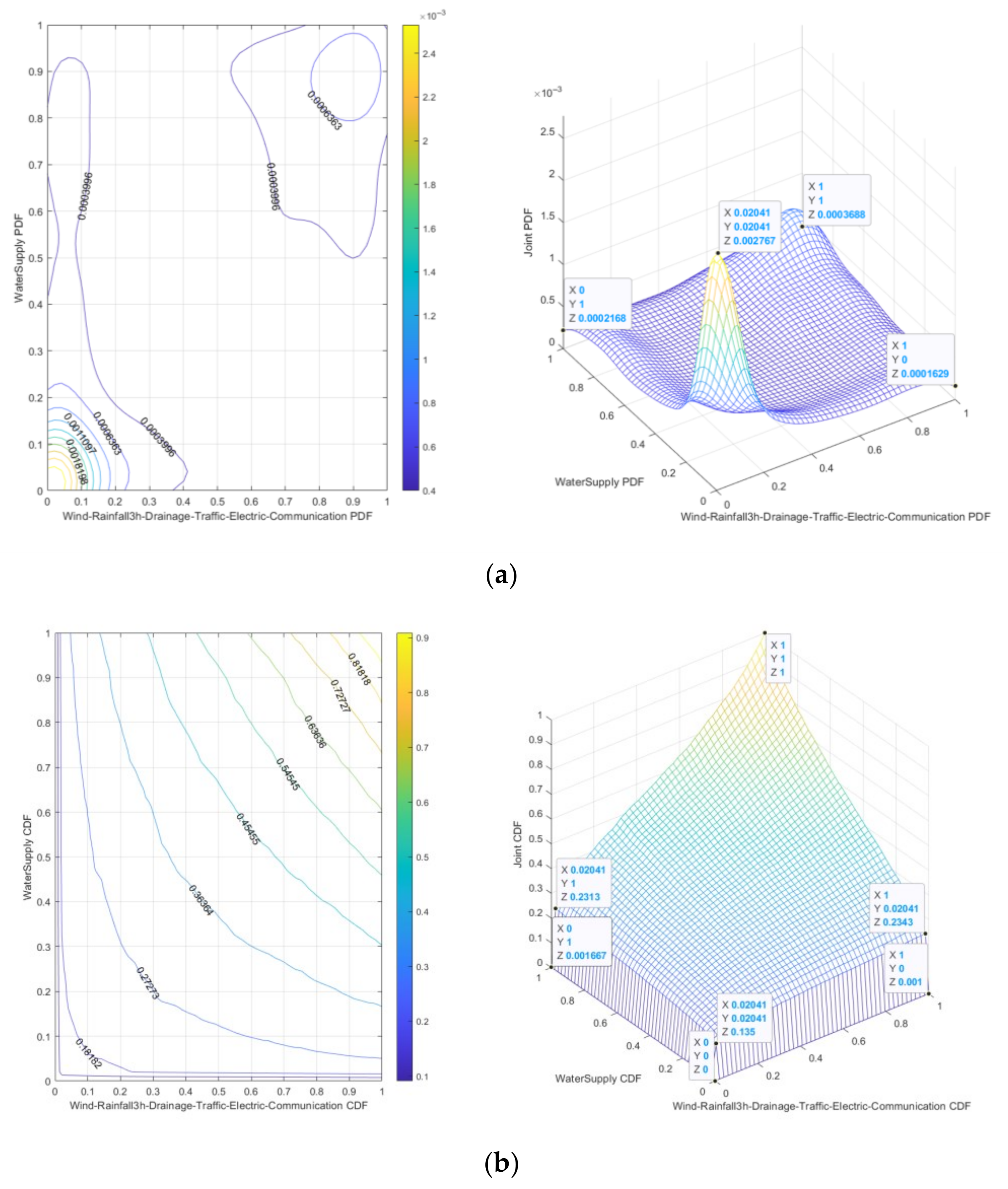
The 3 h Rainfall-Wind speed-Drainage-Traffic-Electric-Communication-Water supply risk is “dark red”, indicating that under the specific conditions of 3 h Rainfall-Wind speed and Drainage-Traffic-Electric-Communication-Water supply, the probability of 3 h Rainfall-Wind speed-Drainage-Traffic-Electric-Communication-Water supply risk is relatively high. It can be seen from Figure 13a that the peak joint probability density is 0.002767, and from Figure 13b that the joint cumulative probability range is 0~0.135, which means that under low-risk conditions, small changes in 3 h Rainfall-Wind speed-Drainage-Traffic-Electric-Communication-Water supply risk may lead to significant increases in risks.
Based on Figure 11, Figure 12 and Figure 13, it can be seen from the dense distribution of contour lines and the three-dimensional significant single peak characteristics that the strong tail correlation dominates the risk coupling effect in the low-risk range, and the joint occurrence of 3 h Rainfall-Wind speed risk and Drainage-Traffic-Electric (3rd-order)/Drainage-Traffic-Electric-Communication (4th-order)/Drainage-Traffic-Electric-Communication-Water supply (5th-order) risk has a high concentration and high probability density. With the increase in risk value range (high risk value range), the independence of 3rd-order, 4th-order, and 5th-order risk increases, the probability density decreases significantly, and the contour becomes sparse, reflecting that under extreme conditions, the joint occurrence probability of risk factors is low. The cumulative probability gradient is steep, indicating that in a short time, a small fluctuation of 3rd-order, 4th-order, and 5th-order risk can trigger the crossing of the risk threshold. The gradient of cumulative probability is slowing down, indicating that the accumulation of risk is approaching saturation.
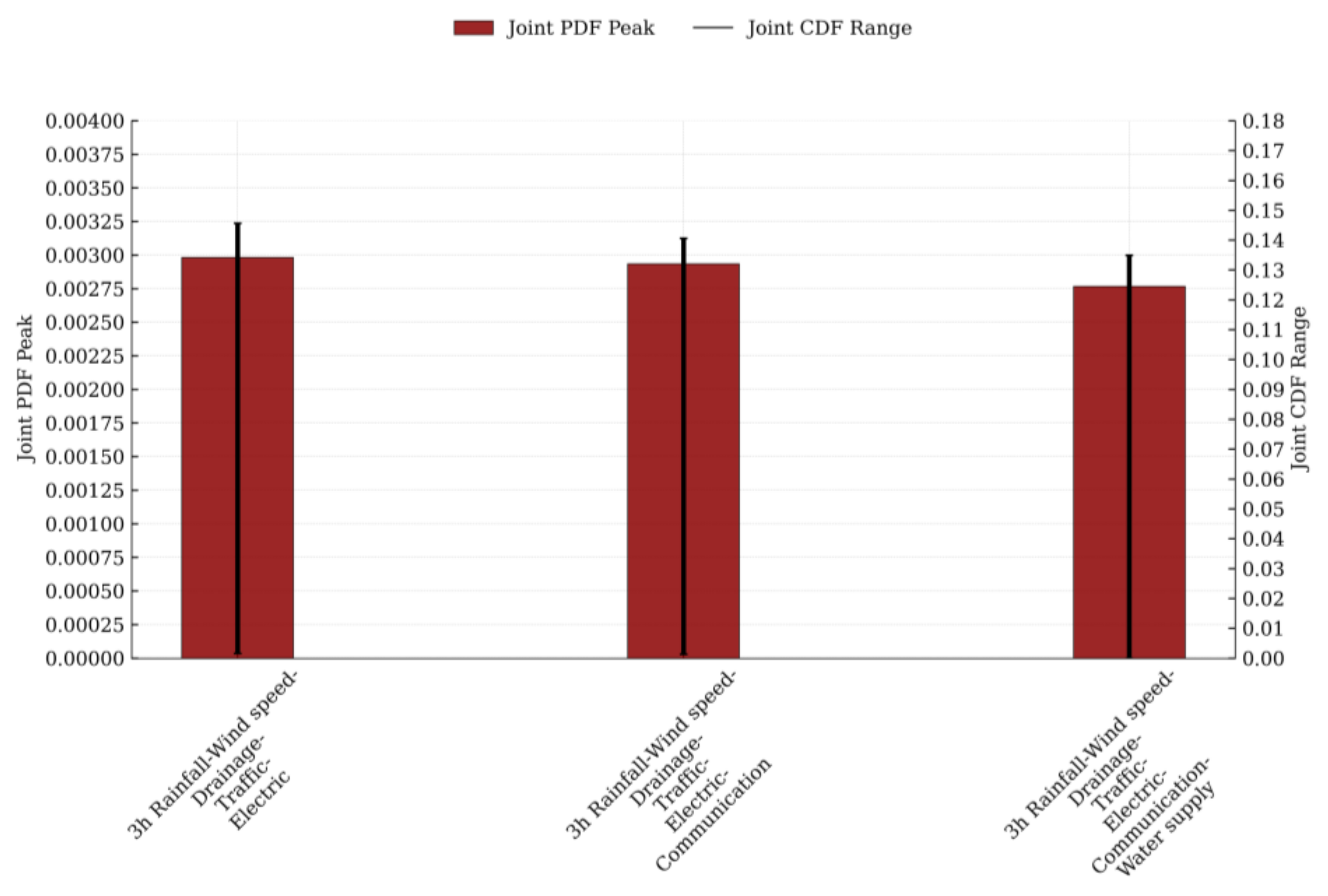
The peak ranks of joint probability density for 3rd-order to 5th-order risk evolution in urban lifeline Natech events are as follows: 3 h Rainfall-Wind speed-Drainage-Traffic-Electric, 3 h Rainfall-Wind speed-Drainage-Traffic-Electric-Communication, and 3 h Rainfall-Wind speed-Drainage-Traffic-Electric-Communication-Water supply. Correspondingly, the scope ranks of joint cumulative probability for 3rd-order to 5th-order risk evolution exhibit the same ordering pattern. Figure 14 illustrates both the peak joint probability density and the range of joint cumulative probability across these sequences.
Under 3 h Rainfall-Wind speed scenarios, each additional link in the chain of risk propagation for urban lifeline technological accidents results in a gradual decline in peak joint probability density—indicating a deceleration in “Risk Spread Velocity”. Simultaneously, the shrinking range of joint cumulative probability signifies a contraction of the “Risk Buffer Zone”. As transmission chains multiply, risk coupling intensifies, ultimately trapping multi-stage urban lifeline Natech risks in a state characterized by slowed progression yet inevitable exposure. Consequently, risk management priorities must shift from reactive “Rapid Repair Mobilization” toward proactive strategies of “Preemptive Decoupling, Zoned Redundancy Design”.
Based on the above analysis, it was found that in the 1st-order risk evolution joint probability distribution of urban lifeline Natech events, only the 1st-order risk of 3 h Rainfall-Wind speed-Drainage is categorized as ‘red’, while all other 1st-order risks are classified as ‘dark red’. From this, it can be concluded that the impact sequence of 3 h Rainfall-Wind speed on urban lifeline risks is as follows: Traffic, Communication, Electric, Water supply, and Drainage. However, in the 2nd-order risk evolution joint probability distribution of urban lifeline Natech events, all risks are categorized as ‘dark red’. Therefore, it can be inferred that the 1st-order risk of 3 h Rainfall-Wind speed-Drainage is a primary influencing factor leading to other 2nd-order risks. Specifically, the impact sequence of 3 h Rainfall-Wind speed-Drainage on other urban lifeline risks is as follows: Traffic, Communication, Electric, and Water supply. Additionally, under 3 h Rainfall-Wind speed scenarios, the extent of Water supply’s impact on Traffic risks surpasses the influence of Electric on Communication, Electric on Water supply, and Communication on Traffic. By analogy, the 1st-order risk of 3 h Rainfall-Wind speed-Drainage is also one of the main factors contributing to 3rd-order to 5th-order risks. The Henan Zhengzhou “7·20” Extraordinary Rainfall Disaster Investigation Report mentions that ‘urban rainfall far exceeded drainage capacity, causing severe flooding of residential community public facilities; multiple regions experienced blackouts, water and network outages, and road traffic disruptions.’ This confirms that the above analysis aligns with real-world conditions, demonstrating the practical application value of the joint probability distribution model (MdC Copula function) for risk evolution of urban lifeline Natech events.
The strong tail correlation dominates the risk coupling effect in the low range of 1st-order to 5th-order risks of the urban lifeline Natech event, while the independence of variables in the high range is enhanced. Under extreme conditions, the probability of the joint occurrence of risk factors is low, but small fluctuations in risk can trigger a crossing of the risk threshold. The joint probability distribution analysis of the risk evolution of urban lifeline Natech events can help urban lifeline managers understand that under extreme natural hazard conditions, the focus of risk management for urban lifeline Natech events may need to shift to reducing the likelihood of risk occurrence, rather than just focusing on the accumulation of risks.

5.3. Joint Probability Prediction of 3 h Rainfall-Wind Speed-Urban Lifelines Risk Evolution

To ensure the stability and reliability of probability predictions for risk evolution in urban lifeline Natech events, the iteration count was designed to be 10 × 104. Based on empirical principles, the burn-in period can be set as 10~20% of the total iterations, i.e., a burn-in period of 2 × 10⁴. The evolution data of rainfall and wind speed risk use empirical quantiles (instead of fixed 0.5), while the evolution data of Traffic, Electric, Communication, Drainage, and Water supply risk are mapped to estimated values of [0, 1] using theoretical means. Markov Chains for the joint probability distribution of 1st-order to 5th-order risk evolution in urban lifeline Natech events (3-D to 7-D Copula functions) were constructed using the M-H algorithm and Gibbs sampling.
The convergence diagnostic metrics of the Markov Chains calculated via the Gelman–Rubin method are presented in Table 8. As shown in Table 8, both the M-H algorithm and Gibbs sampling can generate Markov Chains with stable convergence for joint probability distributions of risk evolution in urban lifeline Natech events, but Gibbs sampling outperforms the M-H algorithm. Therefore, Monte Carlo integration was performed on the converged and stable Markov Chains generated by Gibbs sampling to achieve joint probability predictions for 1st-order to 5th-order risk evolution in urban lifeline Natech events.
Under rainstorm and gale scenarios, the inherent differences in disaster prevention and resistance capabilities among urban lifeline engineering systems—such as Traffic, Electric, Communication, Water supply, and Drainage—indirectly influence the level of their joint probability of risk evolution. Rainstorms can lead to road flooding, pavement collapse, and traffic signal interruptions. Gales may uproot trees and topple traffic signs, thereby affecting road accessibility. The disaster resilience capacity of traffic systems is constrained by multiple factors. On one hand, the design standards for infrastructure such as roads and bridges may fail to fully withstand extreme weather events. On the other hand, the complexity of traffic networks makes localized damage prone to triggering chain reactions, resulting in widespread congestion or system paralysis. Electric systems typically possess a certain level of disaster resilience through windproof and waterproof designs, owing to their high redundancy configuration. For instance, critical electric transmission lines undergo intensified inspections and maintenance during disaster warning phases to promptly eliminate potential hazards. The disaster resilience of communication systems primarily manifests in the redundancy of their network architecture and emergency support capabilities. Communication networks typically employ technologies such as multi-path transmission and backup nodes to ensure that basic communication can be maintained even when partial facilities are damaged. Additionally, during disasters, telecommunication authorities can rapidly activate emergency measures—including mobile communication vehicles and satellite communications—to restore communication services. Water supply systems typically achieve a certain level of disaster resilience through flood control, wind resistance designs, and the establishment of backup water supply facilities. During disasters, water authorities can safeguard water security by adjusting supply schemes and activating alternative water sources. The disaster resilience of drainage systems depends on their design standards and maintenance quality. Rainstorms can cause blockages in drainage pipes and damage pump stations, while gales may destroy drainage facilities, impairing drainage efficiency. On one hand, the capacity of drainage pipes may fail to meet the demands of extreme downpours; on the other hand, delayed maintenance and upgrades of the drainage infrastructure can further reduce overall drainage performance. Therefore, by converting the joint probability of risk evolution for Traffic, Electric, Communication, Water supply, and Drainage systems under rainstorm-gale scenarios into concrete numerical values, urban lifeline authorities and emergency management agencies can determine resource allocation priorities and response tiers. This provides a replicable decision-making template for managing safety risks associated with Natech events affecting urban lifelines.

5.3.1. Joint Probability Prediction of 3 h Rainfall-Wind Speed-Urban Lifelines 1st-Order Risk Evolution

The joint probability prediction for the 1st-order risk evolution of 3 h Rainfall-Wind speed-Urban Lifeline systems is shown in Figure 15. By analyzing Figure 15 in conjunction with Figure 7, it can be observed that under a 3 h Rainfall of 341.9 mm and a Wind speed of 4.499 m/s:
(1)
The 3 h Rainfall-Wind speed-Traffic risk is classified as “dark red”, with a joint probability density of 0.0001008 and a joint cumulative probability of 0.1253.
(2)
The 3 h Rainfall-Wind speed-Electric risk is classified as “dark red”, with a joint probability density of 0.00009835 and a joint cumulative probability of 0.1262.
(3)
The 3 h Rainfall-Wind speed-Communication risk is classified as “dark red”, with a joint probability density of 0.00009894 and a joint cumulative probability of 0.1267.
(4)
The 3 h Rainfall-Wind speed-Water supply risk is classified as “dark red”, with a joint probability density of 0.00009783 and a joint cumulative probability of 0.1268.
(5)
The 3 h Rainfall-Wind speed-Drainage risk is classified as “red”, with a joint probability density of 0.0001004 and a joint cumulative probability of 0.1274.
According to the above results, the “red” evolution of 3 h Rainfall-Wind speed-Drainage risk has the largest cumulative probability, followed by the probability density. Although the risk level is the lowest, it is the first line of defense for Traffic, Electric, Communication and Water supply risk management. 3 h Rainfall-Wind speed-Traffic risk is the “dark red” evolution with the smallest cumulative probability, but its probability density is the largest, indicating that its “dark red” risk consequences are the most serious. The evolution probability of 3 h Rainfall-Wind speed-Water supply, 3 h Rainfall-Wind speed-Communication, 3 h Rainfall-Wind speed-Electric, 3 h Rainfall-Wind speed-Traffic risks as “dark red” decreases in turn, and the consequence severity of the “dark red” risks of 3 h Rainfall-Wind speed-Water supply, 3 h Rainfall-Wind speed-Electric, 3 h Rainfall-Wind speed-Communication, 3 h Rainfall-Wind speed-Traffic gradually increases. Urban lifeline management departments and emergency management agencies can rationally adjust their “attention” toward risk responses based on the ranks of evolutionary probability density and cumulative probability for 1st-order risks associated with urban lifelines during rainstorm and gale.

5.3.2. Joint Probability Prediction of 3 h Rainfall-Wind Speed-Urban Lifelines 2nd-Order Risk Evolution

The joint probability prediction for the 2nd-order risk evolution of 3 h Rainfall-Wind speed-Urban Lifeline systems is shown in Figure 16. By analyzing Figure 16 in conjunction with Figure 7, it can be observed that under a 3 h Rainfall of 341.9 mm and a Wind speed of 4.499 m/s:
(1)
The 3 h Rainfall-Wind speed-Drainage-Traffic risk is classified as “dark red”, with the joint probability density of 0.00006339 and the joint cumulative probability of 0.06365.
(2)
The 3 h Rainfall-Wind speed-Drainage-Electric risk is classified as “dark red”, with the joint probability density of 0.00006189 and the joint cumulative probability of 0.06365.
(3)
The 3 h Rainfall-Wind speed-Drainage-Communication risk is classified as “dark red”, with the joint probability density of 0.00006010 and the joint cumulative probability of 0.06392.
(4)
The 3 h Rainfall-Wind speed-Drainage-Water supply risk is classified as “dark red”, with the joint probability density of 0.00006125 and the joint cumulative probability of 0.06403.
(5)
The 3 h Rainfall-Wind speed-Water supply-Traffic risk is classified as “dark red”, with the joint probability density of 0.00006118 and the joint cumulative probability of 0.06313.
(6)
The 3 h Rainfall-Wind speed-Electric-Water supply risk is classified as “dark red”, with a joint probability density of 0.00005892 and a joint cumulative probability of 0.06364.
(7)
The 3 h Rainfall-Wind speed-Communication-Traffic risk is classified as “dark red”, with the joint probability density of 0.00006198 and the joint cumulative probability of 0.06301.
(8)
The 3 h Rainfall-Wind speed-Electric-Communication risk is classified as “dark red”, with the joint probability density of 0.00006027 and the joint cumulative probability of 0.06284.
According to the above results, the evolution probability of 3 h Rainfall-Wind speed-Drainage-Water supply, 3 h Rainfall-Wind speed-Drainage-Communication, 3 h Rainfall-Wind speed-Drainage-Electric, 3 h Rainfall-Wind speed-Drainage-Traffic risks as “dark red” decreases in turn, but the severity of the consequences of 3 h Rainfall-Wind speed-Drainage-Communication, 3 h Rainfall-Wind speed-Drainage-Water supply, 3 h Rainfall-Wind speed-Drainage-Electric, 3 h Rainfall-Wind speed-Drainage-Traffic “dark red” risks increase gradually. The evolution probability of 3 h Rainfall-Wind speed-Electric-Water supply, 3 h Rainfall-Wind speed-Water supply-Traffic, 3 h Rainfall-Wind speed-Communication-Traffic, 3 h Rainfall-Wind speed-Electric-Communication risks to be “dark red” decrease in turn, but the severity of the “dark red” risk consequences of 3 h Rainfall-Wind speed-Electric-Water supply, 3 h Rainfall-Wind speed-Electric-Communication, 3 h Rainfall-Wind speed-Water supply-Traffic, 3 h Rainfall-Wind speed-Communication-Traffic gradually increase. Based on the “red” risk evolution probability of 3 h Rainfall-Wind speed-Drainage, the 2nd-order “dark red” risk evolution probability of the urban lifeline Natech event is about half of the 1st-order risk evolution probability. Urban lifeline management departments and emergency management agencies can rationally adjust their “attention” toward risk responses based on the ranks of evolutionary probability density and cumulative probability for 2nd-order risks associated with urban lifelines during rainstorm and gale.

5.3.3. Joint Probability Prediction of 3 h Rainfall-Wind Speed-Urban Lifelines 3rd-Order to 5th-Order Risk Evolution

The joint probability predictions for the 3rd-order to 5th-order risk evolution of 3 h Rainfall-Wind speed-Urban Lifeline systems are shown in Figure 17, Figure 18 and Figure 19. By analyzing Figure 17, Figure 18 and Figure 19 in conjunction with Figure 7, it is observed that under a 3 h Rainfall of 341.9 mm and a Wind speed of 4.499 m/s:
(1)
The 3 h Rainfall-Wind speed-Drainage-Traffic-Electric risk is classified as “dark red”, with a joint probability density of 0.0004547 and a joint cumulative probability of 0.03162.
(2)
The 3 h Rainfall-Wind speed-Drainage-Traffic-Electric-Communication risk is classified as “dark red”, with a joint probability density of 0.0003574 and the joint cumulative probability of 0.01626.
(3)
The 3 h Rainfall-Wind speed-Drainage-Traffic-Electric-Communication-Water supply risk is classified as “dark red”, with a joint probability density of 0.0002067 and a joint cumulative probability of 0.008383.
According to the above results, the probability density of 3 h Rainfall-Wind speed-Drainage-Traffic-Electric, 3 h Rainfall-Wind speed-Drainage-Traffic-Electric-Communication, 3 h Rainfall-Wind speed-Drainage-Traffic-Electric-Communication-Water supply risks that are “dark red” shows a decreasing trend, indicating that with the increase in risk transmission chains, the severity of “dark red” risk consequences gradually decreases. The cumulative probability of 3 h Rainfall-Wind speed-Drainage-Traffic-Electric, 3 h Rainfall-Wind speed-Drainage-Traffic-Electric-Communication, 3 h Rainfall-Wind speed-Drainage-Traffic-Electric-Communication-Water supply risks that are “dark red” shows a “half” trend, indicating that with the increase in risk transmission chains, the probability of “dark red” risk decreases by 0.5 times. Urban lifeline management departments and emergency management agencies can rationally adjust their “attention” toward risk responses based on the ranks of evolutionary probability density and cumulative probability for 3rd-order to 5th-order risks associated with urban lifelines during rainstorms and gales.
The joint risk evolution probability density and the joint cumulative risk evolution probability can collectively serve as a “Dual-Wheel Drive” mechanism to facilitate cross-departmental coordination in managing Natech event risks for urban lifelines. The joint cumulative risk evolution probability functions as “Decision Directive”, issued by the Urban Lifeline Safe Operation Monitoring Center, serving as the sole trigger for emergency responses by urban lifeline management departments and emergency management agencies. Meanwhile, the joint risk evolution probability density acts as “Execution Directive”, guiding these departments to continuously optimize operational checklists, material inventories, and personnel deployment matrices—establishing a command structure that is “Horizontally Comprehensive and Vertically Thorough”. The joint probability density operates as “Calibration Dial” for emergency resource allocation, while the joint cumulative probability serves as “Graduation Scale” for determining response tiers. By treating the former as a metric for system failure likelihood and a resource intensity benchmark, and the latter as an indicator of risk impact magnitude and response level criteria, urban lifeline management departments and emergency management agencies can transition from “Experience-Based Decision-Making” to “Data--Based Decision-Making”. This achieves “Early Warning, Risk Reduction” “Pre Resource, Avoid Blind Action” “System Differentiation Prevention and Control, Avoid ‘One Size Fits All’”. Thus, the joint risk evolution probability density may be regarded as micro-level adjustment “Knob”, while the joint cumulative probability represents macro-level adjustment “Switch” for Natech risk management. Within this unified theoretical framework, decision-makers can close the loop on critical questions: when, where, and at what level to respond. This approach simultaneously prevents resource wastage and mitigates under-response risks.


6. Conclusions, Recommendation, and Outlook

6.1. Conclusions

Taking the “7·20” rainstorm disaster in Henan Zhengzhou in 2021 as a case study, this research takes 3 h Rainfall and Wind speed as natural hazard data, and Traffic, Electric, Communication, Water supply, and Drainage as risk components of urban lifeline Natech events. The MdC function is employed to construct the joint probability distribution for the risk evolution of urban lifeline Natech events, while the MCMC method is utilized to predict their joint probability. The MdC function effectively quantifies the uncertainty and complexity of risk evolution in urban lifeline Natech events, and the MCMC model captures the stochastic nature of such risks. The integration of MdC functions and MCMC models offers a novel approach and methodology for predicting the evolutionary probabilities of urban lifeline Natech event risks. This provides visual models and results for urban lifeline regulatory managers and foundational theoretical support for risk prediction of urban lifeline Natech events.
(1)
For 1 h, 6 h, and 12 h rainfall, the distribution follows the GEV function; for 3 h rainfall, it follows a Log Normal function, which exhibits the relatively highest number of peaks; for wind speed, the distribution follows the Gamma function. The marginal probability distribution for risk evolution of urban lifeline systems adheres to a reversed Logistic function.
(2)
The optimal joint probability distribution for 3 h Rainfall-Wind speed risk evolution is modeled by the Gumbel Copula function, exhibiting upper-tail dependence. This indicates that the dependency between 3 h Rainfall risk and Wind speed risk intensifies under extreme-risk scenarios. Numerical simulations reveal that in the low-risk domain of 3 h Rainfall-Wind speed, strong tail correlations dominate the risk coupling effect, while in the high-risk domain, variable independence increases. From this, it can be concluded that the risk intensity of 3 h Rainfall is significantly higher than that of Wind speed.
(3)
The optimal joint probability distribution for 3 h Rainfall-Wind speed-Urban Lifeline 1st-order to 5th-order risk evolution is characterized by the Gumbel Copula function, exhibiting upper-tail dependence. This indicates that under extreme-risk scenarios, the dependency between urban lifeline risks and the combined risks of 3 h Rainfall-Wind speed intensifies, and the dependency between 2nd-order to 5th-order Natech event risks and 1st-order to 4th-order risks also strengthens. Numerical simulations reveal that when 3 h Rainfall reaches 341.9 mm and Wind speed is 4.499 m/s, the 1st-order risk of “3 h Rainfall-Wind speed-Traffic, Electric, Communication, and Water supply” is classified as “dark red”, while the 1st-order risk of “3 h Rainfall-Wind speed-Drainage” is “red”. The 2nd-order to 5 h-order risks of “3 h Rainfall-Wind speed-Urban Lifelines” are all “dark red”. These simulations yield the peak joint probability density and range of joint cumulative probabilities for the 1st-order to 5th-order risk evolution of urban lifeline Natech events. Although 3 h Rainfall-Wind speed has the least impact on drainage risk, the 1st-order “red” risk of “3 h Rainfall-Wind speed-Drainage” acts as a “trigger” for the 2nd-order to 3rd-order “dark red” risks. Combined with the Henan Zhengzhou “7·20” Extraordinary Rainstorm Disaster Investigation Report, the analysis results of the joint probability distribution (MdC) for urban lifeline Natech event risk evolution align with real-world observations, demonstrating practical application value.
(4)
Monte Carlo integration was performed on the Markov Chains constructed using Gibbs sampling to model the joint probability distribution of 1st-order to 5th-order risk evolution for urban lifeline Natech events. Numerical simulations were conducted to predict the risk evolution probabilities of 1st-order to 5th-order urban lifeline Natech events under conditions of 3 h Rainfall at 341.9 mm and Wind speed at 4.499 m/s. The 1st-order “red” risk evolution probability of 3 h Rainfall-Wind speed-Drainage was the highest. The 2nd-order “dark red” risk evolution probabilities of 3 h Rainfall-Wind speed-Drainage-Electric and 3 h Rainfall-Wind speed-Drainage-Traffic were identical, indicating that the 1st-order “red” risk of 3 h Rainfall-Wind speed-Drainage had a comparable impact on the 2nd-order “dark red” risks of 3 h Rainfall-Wind speed-Drainage-Electric and 3 h Rainfall-Wind speed-Drainage-Traffic. Based on the 1st-order “red” risk evolution probability of 3 h Rainfall-Wind speed-Drainage, the “dark red” risk evolution probabilities of 2nd-order to 5th-order urban lifeline Natech events decreased by approximately 50% per additional risk transmission chain.

6.2. Recommendation

The theoretical analysis of the joint probability distribution of the 1st-order to 5th-order risk evolution of technical accidents of urban lifelines (Traffic, Electric, Communication, Water supply, Drainage) under the Rainfall-Wind speed scenario can be achieved through the MdC model, which can help urban planning departments and urban lifeline management departments better understand the impact of extreme weather events such as rainstorms and gales on the urban lifeline system. The key work of risk management of urban lifeline Natech events may need to shift to reducing the possibility of risk occurrence, rather than just focusing on the accumulation of risk, so as to optimize the design of natural disaster prevention and improve the resilience of urban lifelines. Therefore, enhancing the disaster resilience of urban lifeline systems against extreme weather conditions such as heavy rainfall and strong winds—while mitigating technical accident risks and optimizing natural hazard defense designs—can be achieved through three key approaches: urban planning, management coordination, and technological innovation. For instance, the rational zoning of urban functions with dedicated safety buffer zones should prioritize siting lifeline infrastructure in elevated areas with superior drainage and wind resistance capabilities, supplemented by protective barriers to avoid concentrated deployment in disaster-prone regions. A cross-departmental information-sharing platform should be established to enable the real-time exchange of meteorological warnings and operational data from lifeline facilities, coupled with multi-agency joint emergency drills to improve coordinated response capabilities during extreme weather events. Additionally, intelligent monitoring systems should be deployed to collect real-time operational data from lifeline assets, leveraging big data analytics and artificial intelligence to develop predictive risk models that anticipate risk evolution trends proactively.
The quantitative prediction of the joint probability of the 1st-order to 5th-order risk evolution of technical accidents of urban lifelines (Traffic, Electric, Communication, Water supply, Drainage) under the Rainfall-Wind speed scenario can be achieved through the MCMC model, which can provide a scientific basis for the urban lifeline management department and emergency management department to achieve cross sectoral coordination (such as defining the responsibilities and action steps under different risk levels), and can provide a theoretical basis for the urban lifeline management department and emergency management department to implement effective emergency management measures (such as emergency resource reserve and dispatching, risk prevention and control focus confirmation and barrier establishment). For example, the traffic department can adjust the traffic signal control strategy in advance according to the risk situation of the Electric and Communication system to ensure smooth traffic. According to the prediction results, deploying rescue teams, reserving materials and equipment in high-risk areas in advance should be conducted to ensure rapid response in case of accidents. To mitigate the domino effect of risk transmission stemming from potential technical accidents in urban lifelines triggered by extreme weather events like rainstorm and gale, implementing technical upgrades and retrofitting for lifeline infrastructure systems should be conducted. For example, incorporating redundant designs and distributed backup strategies into power and communication networks to enhance their disaster resilience and recovery capabilities can be performed.

6.3. Outlook

This study primarily analyzes the evolution probability of technical accident risks for urban lifelines (Traffic, Electric, Communication, Drainage, and Water supply) under Rainfall and Wind speed scenarios. For other single or compound natural disaster scenarios involving different combinations of urban lifeline systems, further research can be conducted based on the established MdC-MCMC model. Within the complex interplay between natural disasters and urban lifeline systems, there may exist unidentified risk transmission chains and interaction mechanisms, leading to discrepancies between model assumptions and real-world conditions. Urban lifeline Natech events involve multi-source data, including natural hazard datasets and infrastructure information, where data uncertainty affects input precision. Due to the diversity of natural disaster types and intensities, geographical heterogeneity in lifeline system configurations, and socioeconomic disparities, findings from specific cities or contexts may not directly generalize to other regions.
For example, cities located in plains are vulnerable to natural disasters such as floods and rainstorms, which can lead to severe urban waterlogging. This disrupts the normal operation of critical infrastructure systems—including electric, communication, and traffic—potentially triggering cascading failures. Coastal cities primarily face threats from typhoons, tsunamis, and storm surges; for example, typhoons and storm surges may damage electric lines and communication base stations. Economically developed cities like Beijing, Shanghai, and Shenzhen typically invest more resources in planning, constructing, and maintaining their vital infrastructure systems, thereby reducing the risk of Natech events. In contrast, economically underdeveloped regions—such as Zhengzhou and Luoyang—often suffer from unscientific urban infrastructure planning, aging equipment, and inadequate maintenance due to funding constraints, significantly increasing the likelihood of Natech events. Therefore, in further research, it is essential to re-implement the joint probability prediction (MCMC) of urban lifeline Natech event risk evolution. This should be accomplished by first resetting the marginal probability distributions of natural disasters and urban lifeline risk evolution, as well as their joint probability distribution (MdC).
The main limitations of this study lie in two aspects: First, it only investigates the joint probability distribution and probability prediction of risk evolution from the perspective of the spatial evolution mechanism (parallel and synergistic effects) of urban lifeline Natech event risks, while failing to consider the temporal evolution mechanism (superposition effect) of such risks. Second, it focuses solely on the risk levels (blue, yellow, orange, red, deep red) of urban lifeline Natech events when studying the joint probability distribution and probability prediction of risk evolution, without accounting for the physical risk thresholds associated with technological accidents in urban lifelines and their domino effects under natural disaster chain scenarios.
In subsequent research, emphasis will be placed on systematically collecting and analyzing temporal parameter data pertaining to the risk evolution of urban lifeline Natech events. This includes capturing the risk status of urban lifelines over continuous time periods within natural disaster chain scenarios, as well as the domino effects of technological accidents occurring in urban lifelines over continuous durations. Building upon the establishment of a comprehensive database integrating both spatial and temporal dimensions of urban lifeline Natech event risk evolution, future work aims to refine the joint probability distribution and predictive models for such risks—taking the physical risk thresholds of these events as a key research perspective. The ultimate goal is to enhance the practical applicability of multivariate Copula functions and Markov Chain Monte Carlo (MCMC) methods in studying the probability dynamics of urban lifeline Natech event risk evolution.

Author Contributions

Methodology, investigation, formal analysis, visualization, software, data curation, writing—original draft preparation, S.L. Conceptualization, supervision, writing reviewing and editing, Y.S. All authors have read and agreed to the published version of the manuscript.

Funding

This research received no external funding.

Institutional Review Board Statement

Not applicable.

Informed Consent Statement

Not applicable.

Data Availability Statement

The manuscript provides data and the MATLAB code supporting the results of this study, and the corresponding author can provide complete data.

Conflicts of Interest

The authors declare no conflicts of interest in submitting to and publishing in this journal.

Appendix A

Table A1. Marginal probability distribution function fitting of Rainfall and Wind speed risk evolution.
DataDistribution TypePDEK-SParameter
D Valuep ValueCritical Value
1 h RainfallNormal16.07010.319400.1741μ = 12.7377 σ = 26.9310
Log Normal3.21660.07220.6809μ = 1.5631 σ = 1.5206
Gamma4.62940.10370α = 0.6257 β = 20.3573
GVE2.53910.06930.4959α = 3.3397 β = 4.0779 γ = 0.8219
Rayleigh37.26590.59880.7287σ = 21.0657
Weibull2.80620.07010.9051α = 9.8465 β = 0.7198
Exp9.74050.16740.0581λ = 0.0785
3 h RainfallNormal14.85180.279500.1674μ = 35.2939 σ = 60.0517
Log Normal1.85460.06090.8116μ = 2.6757 σ = 1.4027
Gamma5.38600.10580α = 0.6830 β = 51.6783
GVE1.96260.05150.4223α = 9.5668 β = 11.1097 γ = 0.8403
Rayleigh32.27750.52790.9122σ = 49.2538
Weibull3.58970.07910.5730α = 28.8020 β = 0.7547
Exp9.36500.18020.0239λ = 0.0283
6 h RainfallNormal14.14190.25580.00020.1637μ = 67.0377 σ = 99.4476
Log Normal2.26340.07740.5731μ = 3.2803 σ = 1.5039
Gamma4.98040.12090α = 0.6590 β = 101.7302
GVE1.86330.06420.2453α = 17.4389 β = 21.2346 γ = 0.8914
Rayleigh28.90250.51100.7561σ = 84.8053
Weibull3.62370.09090.5864α = 54.7154 β = 0.7439
Exp9.49620.20010.0067λ = 0.0149
12 h RainfallNormal13.32020.24680.00020.1592μ = 126.7630 σ = 160.8761
Log Normal2.99150.08080.5021μ = 4.0266 σ = 1.3312
Gamma6.70750.13890α = 0.7358 β = 172.2833
GVE2.49450.07600.1086α = 31.2223 β = 36.4387 γ = 1.0613
Rayleigh27.02050.47320.7639σ = 144.8275
Weibull5.36960.11450.2726α = 109.7840 β = 0.7942
Exp10.00940.20370.0039λ = 0.0079
Wind speedNormal4.12540.09750.46240.1592μ = 1.9767 σ = 0.9212
Log Normal2.33550.05830.7403μ = 0.5559 σ = 0.5588
Gamma1.64350.04990.3437α = 4.1427 β = 0.4772
GVE1.82670.07440.9458α = 1.5710 β = 0.7596 γ = −0.0489
Rayleigh2.43140.07440.7862σ = 1.5421
Weibull2.87820.06100.854α = 2.2308 β = 2.2539
Exp11.44950.28360λ = 0.5059
Note: The bold and underlined text indicates the optimal marginal probability distributions.
Table A2. Joint probability distribution function fitting of 3 h Rainfall-Wind speed-Urban lifeline 1st-order risk evolution.
DataCopula TypeRMSEAICBICParameter
3 h Rainfall-Wind speed-TrafficGaussian Copula0.12311.89544.1858θ = −0.0492
t-Copula0.12662.25156.8324θ = −0.0845
Gumbel Copula0.0908−15.8264−13.5360θ = 1.4453
Clayton Copula0.11891.51453.8049θ = 0.01
Frank Copula0.0824207.4850209.7754θ = 4.9632
Joe Copula0.1189115.8273118.1177θ = 1.01
3 h Rainfall-Wind speed-Electric Gaussian Copula0.14321.12333.4137θ = 0.1411
t-Copula0.14582.96687.5477θ = 0.1070
Gumbel Copula0.1197−22.4486−20.1581θ = 1.5490
Clayton Copula0.1432−0.64271.6478θ = 0.1948
Frank Copula0.1110182.9304185.2208θ = 5.3455
Joe Copula0.1527113.6328115.9233θ = 1.01
3 h Rainfall-Wind speed-CommunicationGaussian Copula0.14031.87134.1618θ = 0.05487
t-Copula0.14133.68868.2695θ = 0.0430
Gumbel Copula0.1111−20.1673−17.8768θ = 1.5267
Clayton Copula0.14321.97234.2627θ = 0.0170
Frank Copula0.1015192.6090194.8994θ = 5.3002
Joe Copula0.1436114.3671116.6576θ = 1.01
3 h Rainfall-Wind speed-Water supplyGaussian Copula0.13801.93854.2289θ = −0.0374
t-Copula0.13743.93178.5127θ = −0.0285
Gumbel Copula0.1081−16.6466−14.3561θ = 1.4620
Clayton Copula0.13500.46692.7574θ = 0.01
Frank Copula0.1008198.2407200.5311θ = 5.0662
Joe Copula0.1349114.7997117.0902θ = 1.01
3 h Rainfall-Wind speed-drainageGaussian Copula0.13271.90044.1909θ = −0.0480
t-Copula0.13193.88798.4688θ = −0.0360
Gumbel Copula0.1075−14.5584−12.2679θ = 1.4119
Clayton Copula0.12920.54252.8329θ = 0.01
Frank Copula0.1015208.2358210.5263θ = 4.8621
Joe Copula0.1292115.2209117.5114θ = 1.01
Note: The bold and underlined text represents the optimal joint probability distribution.
Table A3. Joint probability distribution function fitting of 3 h Rainfall-Wind speed-Urban lifeline 2nd-order risk evolution.
DateCopula TypeRMSEAICBICParameter
3 h Rainfall-Wind speed-Drainage-TrafficGaussian Copula0.24152.06744.3578θ = −0.0413
t-Copula0.24053.83248.4133θ = −0.0156
Gumbel Copula0.2261−9.9577−7.6672θ = 1.2683
Clayton Copula0.23891.98084.2713θ = 0.01
Frank Copula0.2134284.3746286.6651θ = 4.9178
Joe Copula0.2390135.7888138.0793θ = 1.01
3 h Rainfall-Wind speed-Drainage-ElectricGaussian Copula0.25502.12014.4106θ = −0.0521
t-Copula0.25323.95298.5338θ = −0.0181
Gumbel Copula0.2393−8.8085−6.5180θ = 1.2463
Clayton Copula0.25181.90804.1984θ = 0.01
Frank Copula0.2249303.7079305.9984θ = 4.8225
Joe Copula0.2519136.0335138.3240θ = 1.01
3 h Rainfall-Wind speed-Drainage-CommunicationGaussian Copula0.26044.43346.7239θ = 0.2119
t-Copula0.26733.20187.7827θ = 0.0718
Gumbel Copula0.2556−12.6281−10.3376θ = 1.2935
Clayton Copula0.26961.80044.0909θ = 0.0305
Frank Copula0.2412293.1155295.4059θ = 5.2381
Joe Copula0.2706133.7731136.0636θ = 1.01
3 h Rainfall-Wind speed-Drainage-Water supplyGaussian Copula0.21562.58824.8787θ = −0.1264
t-Copula0.21063.65628.2371θ = −0.0370
Gumbel Copula0.1922−9.9184−7.6280θ = 1.2741
Clayton Copula0.20781.18253.4730θ = 0.01
Frank Copula0.1760275.3767277.6671θ = 5.0544
Joe Copula0.2079135.1494137.4398θ = 1.01
3 h Rainfall-Wind speed-Water supply-TrafficGaussian Copula0.21762.10064.3910θ = −0.0546
t-Copula0.21553.94888.5298θ = −0.0201
Gumbel Copula0.1972−10.3805−8.0901θ = 1.2786
Clayton Copula0.21381.60673.8971θ = 0.01
Frank Copula0.1800273.9004276.1909θ = 5.0565
Joe Copula0.2139134.6344136.9249θ = 1.01
3 h Rainfall-Wind speed-Electric-Water supplyGaussian Copula0.23782.08434.3747θ = 0.0508
t-Copula0.23963.94848.5293θ = 0.0181
Gumbel Copula0.2250−10.8539−8.5635θ = 1.2792
Clayton Copula0.24010.98213.2725θ = 0.01
Frank Copula0.2107285.3557287.6461θ = 4.9378
Joe Copula0.2402134.2734136.5638θ = 1.01
3 h Rainfall-Wind speed-Communication-TrafficGaussian Copula0.23672.05054.3409θ = 0.0349
t-Copula0.23803.67138.2523θ = 0.0212
Gumbel Copula0.2202−11.8459−9.5555θ = 1.2953
Clayton Copula0.23832.00014.2906θ = 0.01
Frank Copula0.2017273.8435276.1340θ = 5.2521
Joe Copula0.2384134.8011137.0915θ = 1.01
3 h Rainfall-Wind speed-Electric-CommunicationGaussian Copula0.24872.87865.1691θ = 0.1424
t-Copula0.25333.70548.2863θ = 0.04801
Gumbel Copula0.2412−11.4967−9.2062θ = 1.2869
Clayton Copula0.25531.99774.2882θ = 0.01
Frank Copula0.2279271.7445274.0350θ = 5.1016
Joe Copula0.2554134.9977137.2882θ = 1.01
Note: The bold and underlined text represents the optimal joint probability distribution.
Figure A1. Research framework of urban lifeline Natech event risk probability evolution.
Sustainability 17 07664 g0a1

References

  1. Yadav, N.; Chatterjee, S.; Ganguly, A.R. Resilience of Urban Transport Network-of-Networks under Intense Flood Hazards Exacerbated by Targeted Attacks. Sci. Rep. 2020, 10, 10350. [Google Scholar] [CrossRef] [Scilit]

  2. Chen, Y.; Li, X.; Wang, W.; Wu, G.; Wang, L. Risk Assessment and Prediction of Underground Utility Tunnels Based on Bayesian Network: A Case Study in Beijing, China. J. Circuits Syst. Comput. 2023, 32, 2350096. [Google Scholar] [CrossRef] [Scilit]
  3. Henonin, J.; Russo, B.; Mark, O.; Gourbesville, P. Real-time urban flood forecasting and modelling—A state of the art. J. Hydroinform. 2013, 15, 717–736. [Google Scholar] [CrossRef] [Scilit]
  4. Fu, G.; Kapelan, Z. Flood analysis of urban drainage systems: Probabilistic dependence structure of rainfall characteristics and fuzzy model parameters. J. Hydroinform. 2013, 15, 687–699. [Google Scholar] [CrossRef] [Scilit]
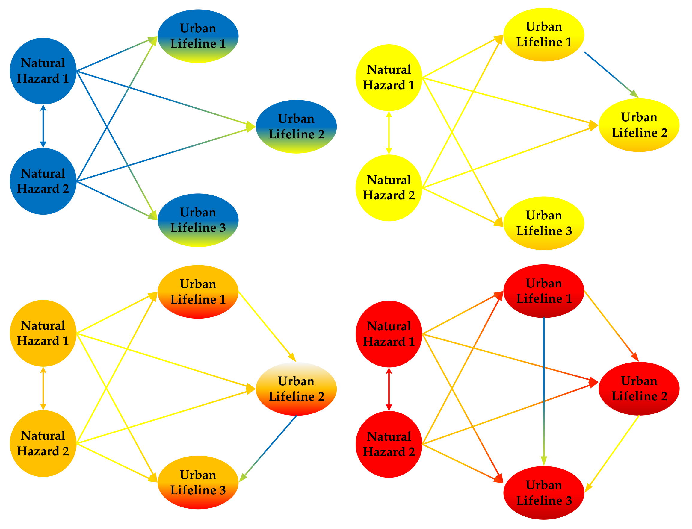
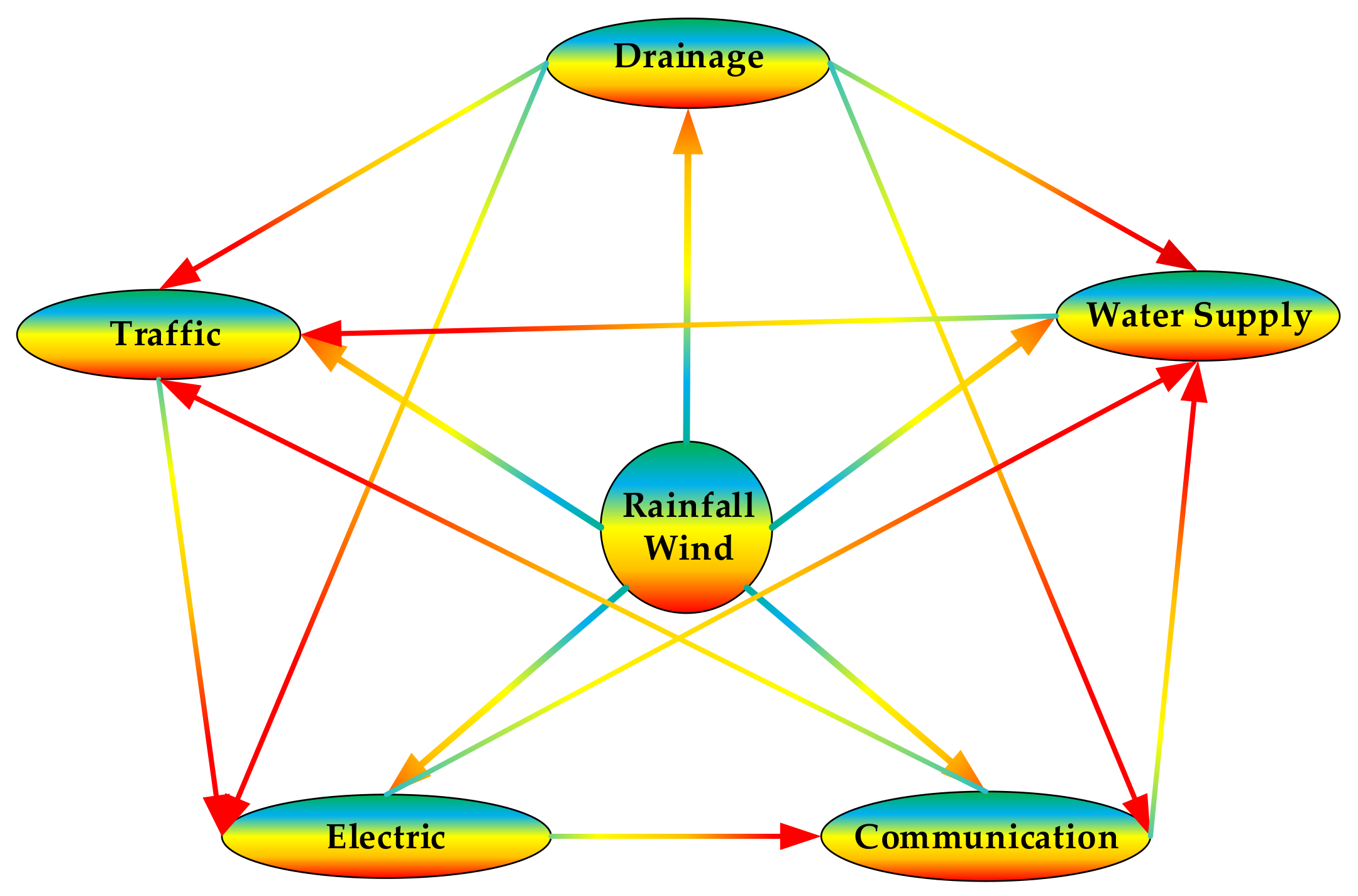
  5. Koukoui, N.; Gersonius, B.; Schot, P.P.; van Herk, S. Adaptation tipping points and opportunities for urban flood risk management. J. Water Clim. Change 2015, 6, 695–710. [Google Scholar] [CrossRef] [Scilit]
  6. Piadeh, F.; Behzadian, K.; Chen, A.S.; Kapelan, Z.; Rizzuto, J.P.; Campos, L.C. Enhancing urban flood forecasting in drainage systems using dynamic ensemble-based data mining. Water Res. 2023, 247, 120791. [Google Scholar] [CrossRef] [Scilit]
  7. Zheng, Y.; Jing, X.; Lin, Y.; Shen, D.; Zhang, Y.; Yuan, D.; Yu, M.; Zhou, Y. Research on nowcasting prediction technology for flooding scenarios based on data-driven and real-time monitoring. Water Sci. Technol. 2024, 89, 2894–2906. [Google Scholar] [CrossRef] [Scilit]
  8. Ma, N.; Xu, Z.; Wang, Y.; Liu, G.; Xin, L.; Liu, D.; Liu, Z.; Shi, J.; Chen, C. Strategies for Improving the Resiliency of Distribution Networks in Electric Power Systems during Typhoon and Water-Logging Disasters. Energies 2024, 17, 1165. [Google Scholar] [CrossRef] [Scilit]
  9. Bagheri, A.; Zhao, C.; Qiu, F.; Wang, J. Resilient Transmission Hardening Planning in a High Renewable Penetration Era. IEEE Trans. Power Syst. 2019, 34, 873–882. [Google Scholar] [CrossRef] [Scilit]
  10. Wang, H.; Hou, K.; Zhao, J.; Yu, X.; Jia, H.; Mu, Y. Planning-Oriented resilience assessment and enhancement of integrated electricity-gas system considering multi-type natural disasters. Appl. Energy 2022, 315, 118824. [Google Scholar] [CrossRef] [Scilit]
  11. Mao, D.; Wang, P.; Fang, Y.; Ni, L. Securing heat-supply against seismic risks: A two-staged framework for assessing vulnerability and economic impacts in district heating networks. Appl. Energy 2024, 369, 123503. [Google Scholar] [CrossRef] [Scilit]
  12. Li, S.F.; Shang, Y. Research on Risk Conduction Chain of Urban Lifeline Natech Event Based on CN-SD. China Saf. Sci. J. 2025, 35, 200–208. [Google Scholar] [CrossRef]
  13. Huang, K.X. Escalation Probability Prediction and Pre-Control Researchon High-Level Domino Effect of NaTech Events in Chemical Industrial Park. Ph.D. Thesis, South China University of Technology, Guangzhou, China, 2022. [Google Scholar] [CrossRef]
  14. Qin, R.S. Risk Modeling and Quantitative Assessment of Natural-Technological Accidents and Domino Effect. Ph.D. Thesis, University of Science and Technology of China, Hefei, China, 2021. [Google Scholar] [CrossRef]
  15. Zhou, L.; Chen, G.; Zheng, M.; Gao, X.; Luo, C.; Rao, X. Agent-based modeling methodology and temporal simulation for Natech events in chemical clusters. Reliab. Eng. Syst. Saf. 2024, 243, 109888. [Google Scholar] [CrossRef] [Scilit]
  16. Wang, J.; Rong, G.; Li, K.; Zhang, J. Analysis of Characteristics of Dry-Wet Events Abrupt Alternation in Northern Shaanxi, China. Water 2021, 13, 2384. [Google Scholar] [CrossRef] [Scilit]
  17. Li, J.; Zhang, Q.; Chen, Y.D.; Singh, V.P. Future joint probability behaviors of precipitation extremes across China: Spatiotemporal patterns and implications for flood and drought hazards. Glob. Planet. Change 2015, 124, 107–122. [Google Scholar] [CrossRef] [Scilit]
  18. Li, Y.; Sun, J.; Cui, X.; Jia, C.; Chao, J. Probability of rainstorm and flood disasters due to extreme precipitation in Fen River Basin, China. Environ. Sci. Pollut. Res. 2023, 30, 70783–70802. [Google Scholar] [CrossRef] [Scilit]
  19. Deger, I.H.; Esit, M.; Yuce, M.I. Univariate and Bivariate Hydrological Drought Frequency Analysis by Copula Functions. Water Resour. Manag. 2023, 37, 4881–4907. [Google Scholar] [CrossRef] [Scilit]
  20. Huang, Y.; Li, G.; Xiong, M. Stochastic assessment of slope failure run-out triggered by earthquake ground motion. Nat. Hazards 2020, 101, 87–102. [Google Scholar] [CrossRef] [Scilit]
  21. Favereau, M.; Robledo, L.F.; Villalobos, D.; Descote, P. On disasters evacuation modeling: From disruptive to slow-response decisions. Int. J. Disaster Risk Reduct. 2022, 67, 102678. [Google Scholar] [CrossRef] [Scilit]
  22. Khan, M.A.; Faisal, M.; Hashmi, M.Z.; Nazeer, A.; Ali, Z.; Hussain, I. Modeling drought duration and severity using two-dimensional copula. J. Atmos. Sol.-Terr. Phys. 2021, 214, 105530. [Google Scholar] [CrossRef] [Scilit]
  23. Rodrigues, D.T.; Goncalves, W.A.; Spyrides, M.H.C.; de Melo Barbosa Andrade, L.; de Souza, D.O.; de Araujo, P.A.A.; Silva, A.C.N.D.; Silva, C.M.S.E. Probability of occurrence of extreme precipitation events and natural disasters in the city of Natal, Brazil. Urban Clim. 2021, 35, 100753. [Google Scholar] [CrossRef] [Scilit]
  24. Alcantara, A.L.; Ahn, K. Probability Distribution and Characterization of Daily Precipitation Related to Tropical Cyclones Over the Korean Peninsula. Water 2020, 12, 1214. [Google Scholar] [CrossRef] [Scilit]
  25. Kolakovic, S.; Mandic, V.; Stojkovic, M.; Jeftenic, G.; Stipic, D.; Kolakovic, S. Estimation of Large River Design Floods Using the Peaks-Over-Threshold (POT) Method. Sustainability 2023, 15, 5573. [Google Scholar] [CrossRef] [Scilit]
  26. Tong, R.P.; Hu, X.Y.; Yin, X.C.; Guo, Y. Risk Zoo(II): Origin, Evolution and Prospects of Risk Metaphor Theory. China Saf. Sci. J. 2023, 33, 8–15. [Google Scholar] [CrossRef]
  27. Jia, H.; Chen, F.; Du, E.; Wang, L. Drought Vulnerability Curves Based on Remote Sensing and Historical Disaster Dataset. Remote Sens. 2023, 15, 858. [Google Scholar] [CrossRef] [Scilit]
  28. Yamanoi, K.; Oishi, S.; Kawaike, K. Prediction of Spatial Distribution of Debris-Flow Hit Probability Considering the Source-Location Uncertainty. J. Flood Risk Manag. 2025, 18, e70011. [Google Scholar] [CrossRef] [Scilit]
  29. Zhan, W.; Baise, L.G.; Moaveni, B. An uncertainty quantification framework for logistic regression based geospatial natural hazard modeling. Eng. Geol. 2023, 324, 107271. [Google Scholar] [CrossRef] [Scilit]
  30. Inkoom, S.; Sobanjo, J.; Chicken, E. Performance Assessment of Deteriorating Bridge Channels in the Presence of Hurricane Failures: The Competing Risks Scenario. J. Infrastruct. Syst. 2021, 27, 04020041. [Google Scholar] [CrossRef] [Scilit]
  31. Cai, Q.L.; Tu, J.L.; Wang, Z.L.; Lai, C.G. Joint Distribution of Strong Wind and Rainstorm in Donghu Reservoir and its Impact on the Design of Dam Crest Elevation. J. Water Resour. Water Eng. 2022, 33, 117–123+129. [Google Scholar]
  32. Petrovic, A.M.; Lescesen, I.; Radevski, I. Unveiling Torrential Flood Dynamics: A Comprehensive Study of Spatio-Temporal Patterns in the Šumadija Region, Serbia. Water 2024, 16, 19. [Google Scholar] [CrossRef] [Scilit]
  33. Yin, K.Y.; Zhang, Y.M.; Gan, Z.Y.; Li, P.F.; Wan, H.; Huang, R. Analysis of Influencing Factors of Radio Interference on 750kV Transmission Lines Under Different Weather Conditions. High Volt. Eng. 2025, 1–11. [Google Scholar] [CrossRef]
  34. Liu, Y.R.; Li, Y.P.; Ma, Y.; Jia, Q.M.; Su, Y.Y. Development of a Bayesian-copula-based frequency analysis method for hydrological risk assessment—The Naryn River in Central Asia. J. Hydrol. 2020, 580, 124349. [Google Scholar] [CrossRef] [Scilit]
  35. Liu, Q.; Tang, A.; Wang, Z.; Zhao, B. Exploring the road icing risk: Considering the dependence of icing-inducing factors. Nat. Hazards 2023, 115, 2161–2178. [Google Scholar] [CrossRef] [Scilit]
  36. Latif, S.; Simonovic, S.P. Trivariate Probabilistic Assessments of the Compound Flooding Events Using the 3-D Fully Nested Archimedean (FNA) Copula in the Semiparametric Distribution Setting. Water Resour. Manag. 2023, 37, 1641–1693. [Google Scholar] [CrossRef] [Scilit]
  37. Bazrafshan, O.; Zamani, H.; Shekari, M.; Singh, V.P. Regional risk analysis and derivation of copula-based drought for severity-duration curve in arid and semi-arid regions. Theor. Appl. Climatol. 2020, 141, 889–905. [Google Scholar] [CrossRef] [Scilit]
  38. Jha, V.B.; Gujrati, A.; Singh, R.P. Copula based analysis of meteorological drought and catchment resilience across Indian river basins. Int. J. Climatol. 2021, 41, E1137–E1151. [Google Scholar] [CrossRef] [Scilit]
  39. Ullah, H.; Akbar, M. Bivariate Drought Risk Assessment for Water Planning Using Copula Function in Balochistan. Environ. Model. Assess. 2023, 28, 447–464. [Google Scholar] [CrossRef] [Scilit]
  40. Xiao, H.; Zhang, J.; Fang, H. A Copula-based framework for joint encounter and state evolution analysis of urban short-duration rainstorm characteristics. J. Hydrol. 2024, 631, 130823. [Google Scholar] [CrossRef] [Scilit]
  41. Zhong, M.; Wang, J.; Jiang, T.; Huang, Z.; Chen, X.; Hong, Y. Using the Apriori Algorithm and Copula Function for the Bivariate Analysis of Flash Flood Risk. Water 2020, 12, 2223. [Google Scholar] [CrossRef] [Scilit]
  42. Botai, C.M.; Botai, J.O.; Adeola, A.M.; de Wit, J.P.; Ncongwane, K.P.; Zwane, N.N. Drought Risk Analysis in the Eastern Cape Province of South Africa: The Copula Lens. Water 2020, 12, 1938. [Google Scholar] [CrossRef] [Scilit]
  43. Khajehali, M.; Safavi, H.R.; Nikoo, M.R.; Najafi, M.R.; Alizadeh-Sh, R. A copula-based multivariate flood frequency analysis under climate change effects. Sci. Rep. 2025, 15, 146. [Google Scholar] [CrossRef] [Scilit] [PubMed]
  44. Dawkins, L.C.; Osborne, J.M.; Economou, T.; Darch, G.J.C.; Stoner, O.R. The Advanced Meteorology Explorer: A novel stochastic, gridded daily rainfall generator. J. Hydrol. 2022, 607, 127478. [Google Scholar] [CrossRef] [Scilit]
  45. Ossandon, A.; Brunner, M.I.; Rajagopalan, B.; Kleiber, W. A space-time Bayesian hierarchical modeling framework for projection of seasonal maximum streamflow. Hydrol. Earth Syst. Sci. 2022, 26, 149–166. [Google Scholar] [CrossRef] [Scilit]
  46. Liu, W.; Wang, D.; Singh, V.P.; Wang, Y.; Zeng, X.; Ni, L.; Tao, Y.; Wu, J.; Liu, J.; Zou, Y.; et al. A hybrid statistical model for ecological risk integral assessment of PAHs in sediments. J. Hydrol. 2020, 583, 124612. [Google Scholar] [CrossRef] [Scilit]
  47. Ismail, M.S.; Masseran, N. Risk assessment for extreme air pollution events using vine copula. Stoch. Environ. Res. Risk Assess. 2024, 38, 2331–2358. [Google Scholar] [CrossRef] [Scilit]
  48. Bai, X.; Jin, J.; Wu, C.; Zhou, R.; Zhou, Y.; Ning, S.; Cui, Y. Cloud transformation algorithm and Copulas function coupling model for drought hazard comprehensive evaluation. Ecol. Eng. 2023, 187, 106870. [Google Scholar] [CrossRef] [Scilit]
  49. Poonia, N.; Azad, S. A New Statistical Distribution Derived from a Clayton Copula for Modeling Bivariate Processes. J. Hydrometeorol. 2023, 24, 1659–1678. [Google Scholar] [CrossRef] [Scilit]
  50. Ayantobo, O.O.; Wei, J.; Wang, G. Modeling Joint Relationship and Design Scenarios Between Precipitation, Surface Temperature, and Atmospheric Precipitable Water Over Mainland China. Earth Space Sci. 2021, 8, e2020EA001513. [Google Scholar] [CrossRef] [Scilit]
  51. Guo, A.; Chang, J.; Wang, Y.; Huang, Q.; Li, Y. Uncertainty quantification and propagation in bivariate design flood estimation using a Bayesian information-theoretic approach. J. Hydrol. 2020, 584, 124677. [Google Scholar] [CrossRef] [Scilit]
  52. Huang, T.; Merwade, V. Improving Bayesian Model Averaging for Ensemble Flood Modeling Using Multiple Markov Chains Monte Carlo Sampling. Water Resour. Res. 2023, 59, e2023WR034947. [Google Scholar] [CrossRef] [Scilit]
  53. Zhao, Z.; Wang, H.; Yu, C.; Deng, C.; Liu, C.; Wu, Y.; Yan, J.; Wang, C. Changes in spatiotemporal drought characteristics over northeast China from 1960 to 2018 based on the modified nested Copula model. Sci. Total Environ. 2020, 739, 140328. [Google Scholar] [CrossRef] [Scilit]
  54. Men, J.; Chen, G.; Yang, Y.; Reniers, G. An event-driven probabilistic methodology for modeling the spatial-temporal evolution of natural hazard-induced domino chain in chemical industrial parks. Reliab. Eng. Syst. Saf. 2022, 226, 108723. [Google Scholar] [CrossRef] [Scilit]
  55. Chen, Y.J.; Chang, K.; Sheu, J.; Liu, C.; Chang, C.; Chang, C.; Wang, G. Vulnerability-based regionalization for disaster management considering storms and earthquakes. Transp. Res. Pt. E-Logist. Transp. Rev. 2023, 169, 102987. [Google Scholar] [CrossRef] [Scilit]
  56. Vats, D.; Knudson, C. Revisiting the Gelman-Rubin Diagnostic. Stat. Sci. 2021, 36, 518–529. [Google Scholar] [CrossRef] [Scilit]
Figure 1. Risk evolution mechanism of urban lifeline Natech events.
Sustainability 17 07664 g001
Figure 2. Schematic diagram of risk evolution of Urban Lifeline under Rainfall-Wind. Note: The direction of the arrows represents the risk transmission chains.
Sustainability 17 07664 g002
Figure 3. Marginal probability distribution curve of Rainfall-Wind speed risk evolution: (a) 1 h Rainfall; (b) 3 h Rainfall; (c) 6 h Rainfall; (d) 12 h Rainfall; (e) Wind speed. Note: The horizontal axis unit is “mm” in (a–d); the horizontal axis unit is “m/s” in (e).
Sustainability 17 07664 g003aSustainability 17 07664 g003bSustainability 17 07664 g003c
Figure 4. Marginal probability distribution curve of Urban lifeline risk evolution.
Sustainability 17 07664 g004
Figure 5. Prediction algorithm process of urban lifeline Natech event risk evolution probability.
Sustainability 17 07664 g005
Figure 6. Joint probability distribution curve of 3 h Rainfall-Wind speed risk evolution: (a) 3 h Rainfall-Wind speed joint probability density; (b) 3 h Rainfall-Wind speed joint cumulative probability.
Sustainability 17 07664 g006
Figure 7. Joint probability distribution curve of 3 h Rainfall-Wind speed-Urban lifeline 1st-order risk evolution: (a) 3 h Rainfall-Wind speed-Traffic joint probability density; (b) 3 h Rainfall-Wind speed-Traffic joint cumulative probability; (c) 3 h Rainfall-Wind speed-Electric joint probability density; (d) 3 h Rainfall-Wind speed-Electric joint cumulative probability; (e) 3 h Rainfall-Wind speed-Communication joint probability density; (f) 3 h Rainfall-Wind speed-Communication joint cumulative probability; (g) 3 h Rainfall-Wind speed-Water supply joint probability density; (h) 3 h Rainfall-Wind speed-Water supply joint cumulative probability; (i) 3 h Rainfall-Wind speed-Drainage joint probability density; (j) 3 h Rainfall-Wind speed-Drainage joint cumulative probability.
Sustainability 17 07664 g007aSustainability 17 07664 g007bSustainability 17 07664 g007cSustainability 17 07664 g007d
Figure 8. Rank of joint probability distribution of 3 h Rainfall-Wind speed-urban lifeline 1st-order risk evolution.
Sustainability 17 07664 g008
Figure 9. Joint probability distribution curve of 3 h Rainfall-Wind speed-Urban lifeline 2nd-order risk evolution: (a) 3 h Rainfall-Wind speed-Drainage-Traffic joint probability density; (b) 3 h Rainfall-Wind speed-Drainage-Traffic joint cumulative probability; (c) 3 h Rainfall-Wind speed-Drainage-Electric joint probability density; (d) 3 h Rainfall-Wind speed-Drainage-Electric joint cumulative probability; (e) 3 h Rainfall-Wind speed-Drainage-Communication joint probability density; (f) 3 h Rainfall-Wind speed-Drainage-Communication joint cumulative probability; (g) 3 h Rainfall-Wind speed-Drainage-Water supply joint probability density; (h) 3 h Rainfall-Wind speed-Drainage-Water supply joint cumulative probability; (i) 3 h Rainfall-Wind speed-Water supply-Traffic joint probability density; (j) 3 h Rainfall-Wind speed-Water supply-Traffic joint cumulative probability; (k) 3 h Rainfall-Wind speed-Electric-Water supply joint probability density; (l) 3 h Rainfall-Wind speed-Electric-Water supply joint cumulative probability; (m) 3 h Rainfall-Wind speed-Communication-Traffic joint probability density; (n) 3 h Rainfall-Wind speed-Communication-Traffic joint cumulative probability; (o) 3 h Rainfall-Wind speed-Electric-Communication joint probability density; (p) 3 h Rainfall-Wind speed-Electric-Communication joint cumulative probability.
Sustainability 17 07664 g009aSustainability 17 07664 g009bSustainability 17 07664 g009cSustainability 17 07664 g009dSustainability 17 07664 g009eSustainability 17 07664 g009f
Figure 10. Rank of joint probability distribution of 3 h Rainfall-Wind speed-urban lifeline 2nd-order risk evolution.
Sustainability 17 07664 g010
Figure 11. Joint probability distribution curve of 3 h Rainfall-Wind speed-Urban lifeline 3rd-order risk evolution: (a) 3 h Rainfall-Wind speed-Drainage-Traffic-Electric joint probability density; (b) 3 h Rainfall-Wind speed-Drainage-Traffic-Electric joint cumulative probability.
Sustainability 17 07664 g011
Figure 12. Joint probability distribution curve of 3 h Rainfall-Wind speed-Urban lifeline 4th-order risk evolution: (a) 3 h Rainfall-Wind speed-Drainage-Traffic-Electric-Communication joint probability density; (b) 3 h Rainfall-Wind speed-Drainage-Traffic-Electric-Communication joint cumulative probability.
Sustainability 17 07664 g012
Figure 13. Joint probability distribution curve of 3 h Rainfall-Wind speed-Urban lifeline 5th-order risk evolution: (a) 3 h Rainfall-Wind speed-Drainage-Traffic-Electric-Communication-Water supply joint probability density; (b) 3 h Rainfall-Wind speed-Drainage-Traffic-Electric-Communication-Water supply joint cumulative probability.
Sustainability 17 07664 g013
Figure 14. Rank of joint probability distribution of rainstorm and gale and urban lifeline third-order to fifth-order risk evolution.
Sustainability 17 07664 g014
Figure 15. Joint probability prediction of 3 h Rainfall-Wind speed-Urban lifeline 1st-order risk evolution.
Sustainability 17 07664 g015
Figure 16. Joint probability prediction of 3 h Rainfall-Wind speed-Urban lifeline 2nd-order risk evolution.
Sustainability 17 07664 g016
Figure 17. Joint probability prediction of 3 h Rainfall-Wind speed-Urban lifeline 3rd-order risk evolution.
Sustainability 17 07664 g017
Figure 18. Joint probability prediction of 3 h Rainfall-Wind speed-Urban lifeline 4th-order risk evolution.
Sustainability 17 07664 g018
Figure 19. Joint probability prediction of 3 h Rainfall-Wind speed-Urban Lifelines 5th-order risk evolution.
Sustainability 17 07664 g019
Table 1. Marginal probability distribution function fitting of Rainfall and Wind speed risk evolution (partial data).
DataDistribution TypePDEK-SParameter
D Valuep ValueCritical Value
1 h RainfallGVE2.53910.06930.49590.1741α = 3.3397 β = 4.0779 γ = 0.8219
3 h RainfallLog Normal1.85460.06090.81160.1674μ = 2.6757 σ = 1.4027
6 h RainfallGVE1.86330.06420.24530.1637α = 17.4389 β = 21.2346 γ = 0.8914
12 h RainfallGVE2.49450.07600.10860.1592α = 31.2223 β = 36.4387 γ = 1.0613
Wind speedGamma1.64350.04990.34370.1592α = 4.1427 β = 0.4772
Note: See Table A1 for complete data of “Marginal probability distribution function fitting of Rainfall and Wind speed risk evolution”.
Table 2. Joint probability distribution function fitting of 3 h Rainfall-Wind speed risk evolution.
DataCopula TypeRMSEAICBICParameter
3 h Rainfall-Wind speedGaussian Copula0.0228−4.5329−2.2425θ = 0.2926
t-Copula0.0247−9.6260−5.0451θ = 0.2522
Gumbel Copula0.0712−144.7864−142.4959θ = 10
Clayton Copula0.0290−2.7785−0.4880θ = 0.3765
Frank Copula0.0382100.4964102.7869θ = 5.7753
Joe Copula0.0451109.8974112.1879θ = 1.01
Note: The bold and underlined text represents the optimal joint probability distribution.
Table 3. Joint probability distribution function fitting of 3 h Rainfall-Wind speed-Urban lifeline 1st-order risk evolution (partial data).
DataCopula TypeRMSEAICBICParameter
3 h Rainfall-Wind speed-TrafficGumbel Copula0.0908−15.8264−13.5360θ = 1.4453
3 h Rainfall-Wind speed-ElectricGumbel Copula0.1197−22.4486−20.1581θ = 1.5490
3 h Rainfall-Wind speed-CommunicationGumbel Copula0.1111−20.1673−17.8768θ = 1.5267
3 h Rainfall-Wind speed-Water supplyGumbel Copula0.1081−16.6466−14.3561θ = 1.4620
3 h Rainfall-Wind speed-drainageGumbel Copula0.1075−14.5584−12.2679θ = 1.4119
Note: See Table A2 for complete data of “Joint probability distribution function fitting of 3 h Rainfall-Wind speed-Urban lifeline 1st-order risk evolution”.
Table 4. Joint probability distribution function fitting of 3 h Rainfall-Wind speed-Urban lifeline 2nd-order risk evolution (partial data).
DateCopula TypeRMSEAICBICParameter
3 h Rainfall-Wind speed-Drainage-TrafficGumbel Copula0.2261−9.9577−7.6672θ = 1.2683
3 h Rainfall-Wind speed-Drainage-ElectricGumbel Copula0.2393−8.8085−6.5180θ = 1.2463
3 h Rainfall-Wind speed-Drainage-CommunicationGumbel Copula0.2556−12.6281−10.3376θ = 1.2935
3 h Rainfall-Wind speed-Drainage-Water supplyGumbel Copula0.1922−9.9184−7.6280θ = 1.2741
3 h Rainfall-Wind speed-Water supply-TrafficGumbel Copula0.1972−10.3805−8.0901θ = 1.2786
3 h Rainfall-Wind speed-Electric-Water supplyGumbel Copula0.2250−10.8539−8.5635θ = 1.2792
3 h Rainfall-Wind speed-Communication-TrafficGumbel Copula0.2202−11.8459−9.5555θ = 1.2953
3 h Rainfall-Wind speed-Electric-CommunicationGumbel Copula0.2412−11.4967−9.2062θ = 1.2869
Note: See Table A3 for complete data of “Joint probability distribution function fitting of 3 h Rainfall-Wind speed-Urban lifeline 2nd-order risk evolution”.
Table 5. Joint probability distribution function fitting of 3 h Rainfall-Wind speed-Urban lifeline 3rd-order risk evolution.
DateCopula TypeRMSEAICBICParameter
3 h Rainfall-Wind speed-Drainage-Traffic-ElectricGaussian Copula0.26579.040011.3305θ = −0.2370
t-Copula0.25863.57858.1595θ = −0.0469
Gumbel Copula0.2504−5.5596−3.2692θ = 1.1819
Clayton Copula0.2566−0.18612.1043θ = 0.01
Frank Copula0.2395371.9408374.2313θ = 4.7245
Joe Copula0.2568142.0251144.3155θ = 1.01
Note: The bold and underlined text represents the optimal joint probability distribution.
Table 6. Joint probability distribution function fitting of 3 h Rainfall-Wind speed-Urban lifeline 4th-order risk evolution.
DateCopula TypeRMSEAICBICParameter
3 h Rainfall-Wind speed-Drainage-Traffic-Electric-CommunicationGaussian Copula0.29897.18619.4765θ = −0.1725
t-Copula0.29433.85898.4398θ = −0.0245
Gumbel Copula0.2885−5.5421−3.2516θ = 1.1718
Clayton Copula0.29331.52033.8108θ = 0.01
Frank Copula0.2793423.0561425.3465θ = 4.7112
Joe Copula0.2934143.9505146.2410θ = 1.01
Note: The bold and underlined text represents the optimal joint probability distribution.
Table 7. Joint probability distribution function fitting of 3 h Rainfall-Wind speed-Urban lifeline 5th-order risk evolution.
DateCopula TypeRMSEAICBICParameter
3 h Rainfall-Wind speed-Drainage-Traffic-Electric-Communication-Water supplyGaussian Copula0.417314.069116.3596θ = 0.2175
t-Copula0.42063.90388.4847θ = 0.0182
Gumbel Copula0.4182−5.9065−3.6160θ = 1.1634
Clayton Copula0.4207−4.0659−1.7754θ = 0.01
Frank Copula0.4137488.2049490.4953θ = 4.6534
Joe Copula0.4208145.1597147.4501θ = 1.01
Note: The bold and underlined text represents the optimal joint probability distribution.
Table 8. Gelman–Rubin diagnostic for Markov chain convergence.
Dimension34567
M-H1.00201.00151.00131.00201.0021
Gibbs1.00001.00001.00001.00001.0000
Disclaimer/Publisher’s Note: The statements, opinions and data contained in all publications are solely those of the individual author(s) and contributor(s) and not of MDPI and/or the editor(s). MDPI and/or the editor(s) disclaim responsibility for any injury to people or property resulting from any ideas, methods, instructions or products referred to in the content.