Deep Learning Models and Their Ensembles for Robust Agricultural Yield Prediction in Saudi Arabia

Abstract

A crop yield prediction is critical to increase agricultural sustainability because it allows for the more effective use of natural resources, including water, fertilizers, and soil. Accurate yield estimates enable farmers and governments to more accurately manage resources, decreasing waste and minimizing adverse environmental effects such as the degradation of soil and water quality issues. In addition, predictive models serve to alleviate the consequences of climate change by promoting adaptable farming techniques and improving the availability of food by means of early decision-making. Thus, including a crop yield prediction into farming practices is critical for combining productivity and sustainability. In contrast to conventional machine learning models, which frequently require long feature engineering, deep learning may obtain complicated yield-related characteristics directly from initial or merely preprocessed data from different sources. This research paper aims to demonstrate the strength of deep learning models and their ensembles in agricultural yield prediction in Saudi Arabia, where agriculture faces issues such as scarce water resources and harsh climate conditions. We first define and evaluate a Multilayer Perceptron (MLP), a Gated Recurrent Unit (GRU), and a Convolutional Neural Network (CNN) as baseline deep models for the crop yield prediction. Then, we investigate combining these three models based on stacking, blending, and boosting ensemble methods. Finally, we study the uncertainty quantification for the proposed models, which involves a discussion of many enhancements’ techniques. As a result, this research shows that, by applying the right architectures with strong parametrization and optimization techniques, we obtain models that can explain 96% of the variance in the crop yield with a very low uncertainty rate (reaching an MPIW of 0.60), which proves the reliability and trustworthiness of the prediction.

1. Introduction

The rise of crop yield prediction as a crucial research field is intricately connected to the increasing worries about climate change and its effects on worldwide food safety [1,2,3]. With climate patterns growing more erratic and extreme weather events becoming more common, traditional agricultural methods and historical yield data are proving less reliable for predicting future harvests. This doubt forms major risks for the food supply and people’s means of living, especially in areas that depend on farming to a large extent. As a result, there has been an increase in studies aimed at creating precise and reliable crop yield prediction models that take into consideration the intricate interactions among atmospheric parameters, soil aspects, and additional variables. Advanced forecasting methods, frequently driven by machine learning and deep learning, are vital for supporting anticipative adjustment plans, leading agricultural governance, and most importantly protecting universal food offerings amid climate change.

Saudi Arabia’s distinctive susceptibility to climatic change and its ambitious goals for agricultural self-sufficiency have catalyzed the rise of crop yield forecasting as a vital area of concern [4,5,6]. Saudi Arabia, being a mostly arid nation with scarce water resources, encounters substantial difficulties in sustaining and growing its agricultural sector in the face of rising temperatures, heightened evapotranspiration, and unpredictable rainfall patterns. This context has led to an increasing focus on creating sophisticated crop yield prediction models that are customized to the unique environmental conditions of the region. These models, which frequently integrate machine learning and remote sensing technologies, are crucial for optimizing water usage, choosing suitable crop varieties, and applying adaptive agricultural practices. These tools enable Saudi Arabia to improve its food security, foster sustainable farming practices, and alleviate the negative effects of climate change on its agricultural environment through the provision of precise and prompt yield forecasts.

Advanced machine learning methods [7] are being used more and more to maximize crop yields and guarantee food security. Especially, deep learning [8,9,10,11] is becoming increasingly important in farming production because of its ability to evaluate large, complex datasets, such as satellite imaging, weather patterns, and soil characteristics, at far higher speeds and accuracy than previous methods. Since contemporary farming faces new challenges such as variations in the climate, limited supplies of resources, and a demand for greater productivity, deep learning allows accurate forecasts, early identification of crop strain, and efficient decision-making, which will eventually contribute to increased efficiency, fewer waste products, and increasingly sustainable food production systems.

On the other hand, designing crop-specific yield forecasting algorithms can be difficult in countries like Saudi Arabia, in which farming data is frequently insufficient and dispersed. This is owing to a lack of thorough crop-level datasets. Indeed, several small-scale farms and regional agricultural groups lack complete, crop-specific records, rendering it hard to create reliable models for individual crops. Also, acquiring comprehensive information for every plant takes a large amount of time and resources. Therefore, a more broadly applicable approach may be more viable. To solve this, it is promising to switch to multi-crop or collective forecasting of yield strategies, which attempt to forecast total agricultural production or yields from numerous crops at the same time.

To contribute to this emerging topic, the present research is keen to create and assess different deep learning models and their ensembles to forecast crop yields by utilizing an extensive dataset that includes soil, weather, and remote sensing data. The goal is to develop a solid and trustworthy model that can estimate yields accurately, promoting sustainable farming methods. Since the obtained crop-specific data is scarce, it is proposed to use the crop type as a categorical feature in unified deep learning models in order to provide a practical method for learning similar trends throughout crops while also collecting important harvest-specific variances. In particular, the present research presents the following contributions:

• A collection of 38 types of crops with their harvests between 1990 and 2024, as well as multi-source input features such as weather data, vegetation indices, and soil characteristics that are known to influence the plants’ growth and yields.
• Definition, training, and evaluation of a Multilayer Perceptron.
• Definition, training, and evaluation of a Gated Recurrent Unit model.
• Definition, training, and evaluation of a Convolutional Neural Network model.
• Enhancing the three models for better performance and uncertainty quantification.
• Applying different ensemble techniques to the three proposed models and studying their performance.

The outcomes of this research help to significantly improve crop production forecasts, allowing for more effective agricultural planning and smarter resource management. By including an uncertainty quantification, the predictability and trustworthiness of the outcomes are considerably increased, giving stakeholders more confidence in decision-making. The ensuing insights are intended to help promote sustainable and economically viable farming practices. Finally, the insights will help in ensuring global food security for a growing population

2. Materials and Methods

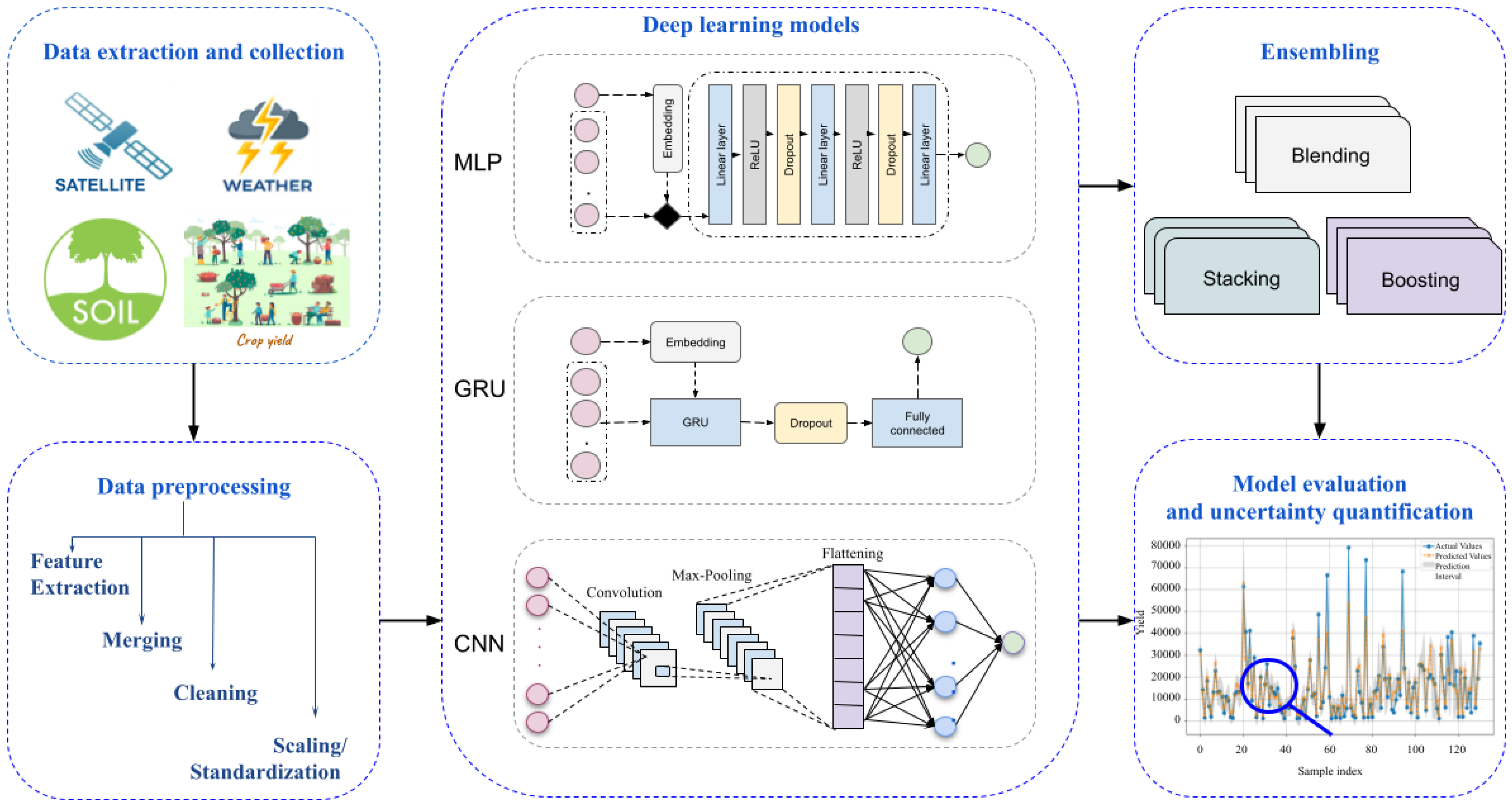
This section describes the proposed framework and its components, as illustrated in Figure 1. We relied on various sources to collect different information useful for an efficient crop yield prediction. Then, we applied careful preprocessing operations, such as cleaning, merging, and scaling, which will ensure data quality, consistency, and suitability for deep learning models and have direct impacts on the prediction performance and reliability. Considering the intricate details of agricultural output predictions, we studied a number of deep learning architectures, including sequence models and spatial feature learners, to determine the best effective representation of the underlying data. We implanted and evaluated three different deep learning architectures: a Multilayer Perceptron (MLP), a Gated Recurrent Unit (GRU), and a Convolutional Neural Network (CNN). Then, we explored their combinations via well experimented ensemble techniques, such as blending, stacking, and boosting.

2.1. Data Extraction and Collection

The first step in the project is gathering agricultural data from various sources that are pertinent to predicting crop yield. Because each data source has its own variability and adds unique information, the crop production prediction depends on a range of data sources. Accurate and trustworthy forecasts depend on combining these disparate datasets and comprehending their variability.

• Yield data: A multitude of information about food, agriculture, and related fields is available from the Food and Agriculture Organization (FAO). FAOSTAT [12] is a thorough statistics database that serves as their main data source. FAOSTAT provides information on a variety of subjects, such as the amounts and values of livestock and the cultivation of crops. FAOSTAT allows users to query and obtain specific information by organizing the data into domains, elements, and items. We downloaded in a CVS file all the information about crop yield in Saudi Arabia in the period from 1990 to 2024. The crops collected count to 38 different plant types.
• Weather data: Weather information is essential for making precise crop yield predictions. Plant growth and development are directly influenced by variables such as temperature, humidity, rainfall, and sun radiation. While real-time data enables well-informed decision-making during the growing season, historical weather patterns aid in the knowledge of areal agricultural trends. Farmers can maximize crop production and reduce losses by optimizing irrigation, fertilization, and harvesting schedules through the analysis of weather data. We developed a Python script (version 3.11.13) that uses NASA’s POWER API [13] to collect daily weather data from 1990 to 2024 for Saudi Arabia by specifying its longitude and latitude. The data, including temperature, precipitation, humidity, and solar radiation, is retrieved using the requests library, and is processed and cleaned using the library Pandas. The processed weather data is then saved into a CSV file for subsequent processing.
• Vegetation indicators: Known as quantitative measurements of the state of plants, vitality, and growth that are generated from satellite imaging, vegetation indices are essential for predicting agricultural yield. Important data regarding photosynthetic activity, the plant matter, and stress conditions of crops over time are captured by indicators, including the Wide Dynamic Range Vegetation Index (WDRVI), Normalized Difference Vegetation Index (NDVI), and Vegetation Condition Index (VCI). These metrics allow for the early detection of abnormalities and the evaluation of growth stages by representing how crops react to environmental elements such as temperature, water accessibility, and the state of the soil. By providing ongoing, extensive, and non-invasive field monitoring, their incorporation into yield forecasting techniques improves accuracy and ultimately facilitates better utilization of resources and agricultural decision-making. We implemented a script in Python that examines the health of Saudi Arabia’s flora using the Earth Engine API. It specifies the study region and the time frame (1990 to 2024), imports the required libraries, and authenticates with Earth Engine. After loading MODIS NDVI data, it computes Saudi Arabia’s mean NDVI over time and transforms it into a Pandas DataFrame. The VCI and an estimated WDRVI are computed by the code after scaling the NDVI values. Lastly, it stores the calculated vegetation indices with the mean NDVI and date data in a CSV file.
• Soil information: Farmers may choose crops, manage their soil, and apply inputs precisely by using detailed soil mapping and analysis, which increases yields and promotes sustainable farming methods. For the crop yield estimation, soil characteristics, including carbon from organic matter, density, clay, silt, and sand contents, are essential components, particularly when evaluating the productivity and health of the soil. These variables are accessible through ISRIC’s SoilGrids project [14], which offers high-resolution worldwide soil data in the GeoTIFF file type. The 0–5 cm depth layer is frequently utilized for investigations concentrating on superficial soil properties, and soilgrids.org provides direct downloads for datasets. These layers can be incorporated into geospatial workflows to extract values unique to a research region, like Saudi Arabia, and indicate average values obtained from the prognostic mapping of soil. By offering a more thorough picture of the soil environment, the inclusion of these factors improves the precision of farming models.

2.2. Data Preprocessing

To guarantee consistency across various datasets, data merging and preparation are needed. From GeoTIFF files, we retrieved the soil data using the rasterio package. We organized this data into a DataFrame using Pandas, handled numerical calculations, and eliminated erroneous data points using numpy. Each soil parameter (pH, organic carbon, sand, clay, and silt) has its average value determined by the code and stored in the DataFrame. In order to make the DataFrame with the average soil parameters easily accessible for additional analysis or usage in other project components, we stored it as a CSV file. This file, along with the three other files containing data about the weather, the vegetation indices, and the crop yield, are then merged, cleaned, and scaled to be ready for use during deep learning. We summarize the main steps performed as follows:

• Feature extraction—This is a vital stage in machine learning and deep learning, where raw data is turned into a set of characteristics that are more useful and relevant to the situation at hand. The process of identifying pertinent details (features) within the initial datasets (GeoTIFF files, satellite data, etc.) for usage in additional analyses or modeling is referred to as extracting features in this setting. Because it streamlines the data, enhances the efficiency of the models, incorporates expertise in the field, and formats the data appropriately for examination, feature extraction is essential in our case. We utilized it at different levels from extracting metrics from GeoTIFF files to extracting information from obtained data like the year from the date.
• Merging—In general, merging in data preprocessing refers to the process of combining two or more datasets into a single dataset. This is particularly performed in our case to combine all the data obtained during the data collection phase.
• Cleaning—Another essential phase in the preprocessing of data is cleaning, which is finding and fixing mistakes, discrepancies, and irregularities in the data. We removed unneeded items and made sure the data was recorded in the right format. Additionally, we identified and handled extreme values that could distort the analysis (filtering outliers). Additionally, since the crop yield is yearly information, we used the extracted feature ‘year’ to merge the different information after taking the average of the different features available in many dates for the year. Then, the date information as well as the duplicates were omitted. Finally, since the soil information is constant and we are studying the farming production in the whole country, we chose to omit the soil information for now and planned to use it when we considered different regions in Saudi Arabia.
• Scaling/Standardization—A critical preliminary process used on input data and/or outputs to enhance the training of models and their performance is scaling or standardization. The process of scaling involves modifying the scope of features or goals. The network may give excessive weight to features with bigger scales if the features have widely disparate ranges (e.g., temperature in degrees Celsius versus yield in kilogram per hectare), which could result in biased learning and ineffective training. By transforming data into ones with a zero ‘mean’ and unit ‘variance’, standardization assists with preventing problems like vanishing or growing gradients and guarantees that all parameters participate similarly throughout optimization. Standardized data also increases the efficacy of methods like weight regularization, batch normalization, and dropout, which facilitates learning and increases the model’s generalizability. We used StandardScaler from scikit-learn for scaling all the features and target data in both the training and testing sets to make sure that features with various scales did not adversely affect the model and hence improved performance.

2.3. Exploratory Data Analysis

Prior to model creation, a thorough exploratory data analysis (EDA) was performed to understand the underlying properties of the collected dataset, identify potential difficulties, and inform subsequent feature engineering and model selection procedures. Following the steps presented in the preprocessing subsection, descriptive statistics (such as means, medians, standard deviations, and quartiles) were calculated to characterize the central tendency and dispersion of numerical variables. The statistical description, illustrated in

Table 1. Statistical description of the collected and integrated dataset.

	Count	Mean	Std	Min	25%	50%	75%	Max
Year	655	2012.58	7.16	2000	2006	2013	2019	2023
Temperature	655	26.09	0.39	25.36	25.83	26	26.43	26.8
Humidity	655	24.63	2.23	21.14	23.35	24.11	25.71	32.11
Precipitation	655	0.11	0.09	0.03	0.05	0.08	0.12	0.41
Solar Radiation	655	22.22	0.35	21.63	21.92	22.36	22.48	22.85
mean_ndvi	655	0.1	0	0.1	0.1	0.1	0.1	0.12
VCI	655	0.31	0.17	0.13	0.21	0.26	0.35	0.88
WDRVI	655	−0.78	0	−0.78	−0.78	−0.78	−0.78	−0.78
Yield	655	15,216.5	13,591.1	96.8	5486.45	12,861.5	20,142.2	85,800.5

, shows key features for numerous variables based on 655 occurrences (obtained after cleaning). After the cleaning process, the data ranges from 2000 to 2023, with weather variables such as temperature, humidity, precipitation, and solar radiation, exhibited a range of distributions. Particularly, temperature and solar radiation have quite little standard deviations (0.39 and 0.35, respectively), suggesting highly uniform values, whereas precipitation exhibits a large relative standard deviation, regardless of having a small average. In addition, ‘mean_ndvi’ has very little variability, with nearly all values at 0.10, whereas ‘WDRVI’ is completely constant at −0.78, making both potentially uninformative for predictive modeling. Lastly, the target parameter, ‘yield’, has a broad spectrum (96.80 to 85,800.50) as well as a significant standard deviation (13,591.05) from its mean (15,216.54), indicating an extremely diverse and biased distribution, which would suggest applying a transformation to it before performing the deep learning.

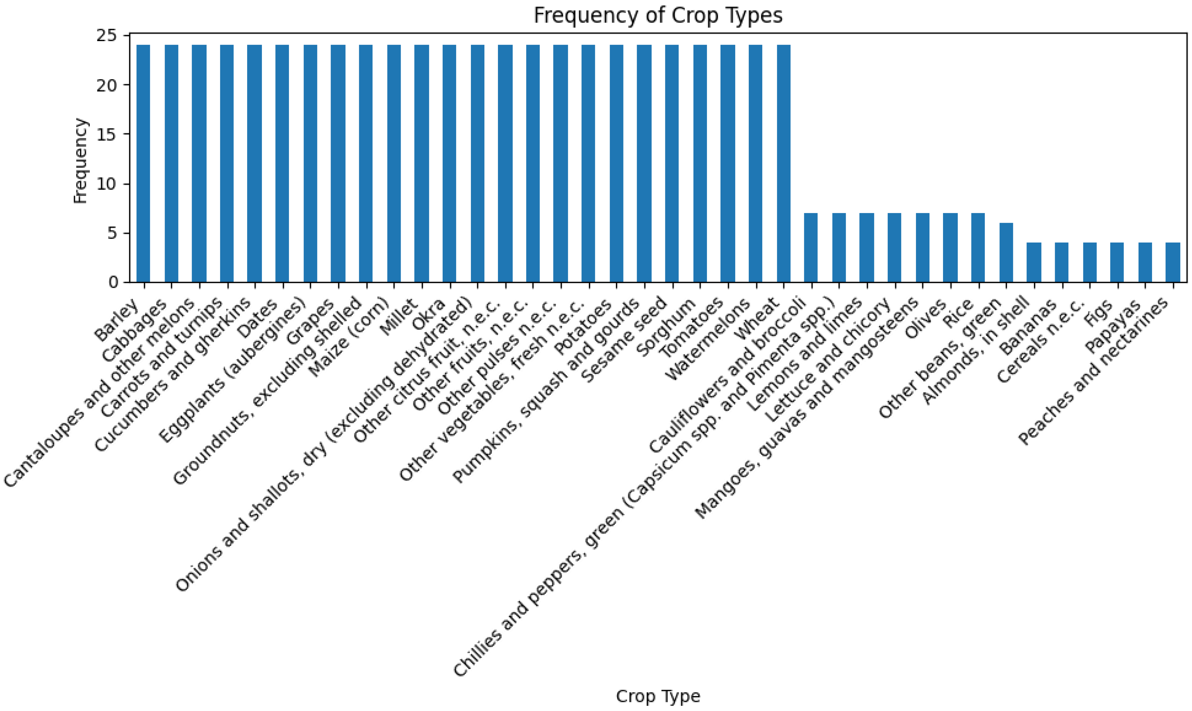
To better comprehend class balance and prevalence, categorical variables have been analyzed based on the distribution of their frequencies. The bar graph in Figure 2 shows the frequency of categories within the ‘crop’ variable before encoding. It shows the presence of 38 different categories with a frequency varying from 4 (for ‘figs’ for example) to 24 (for ‘dates’).

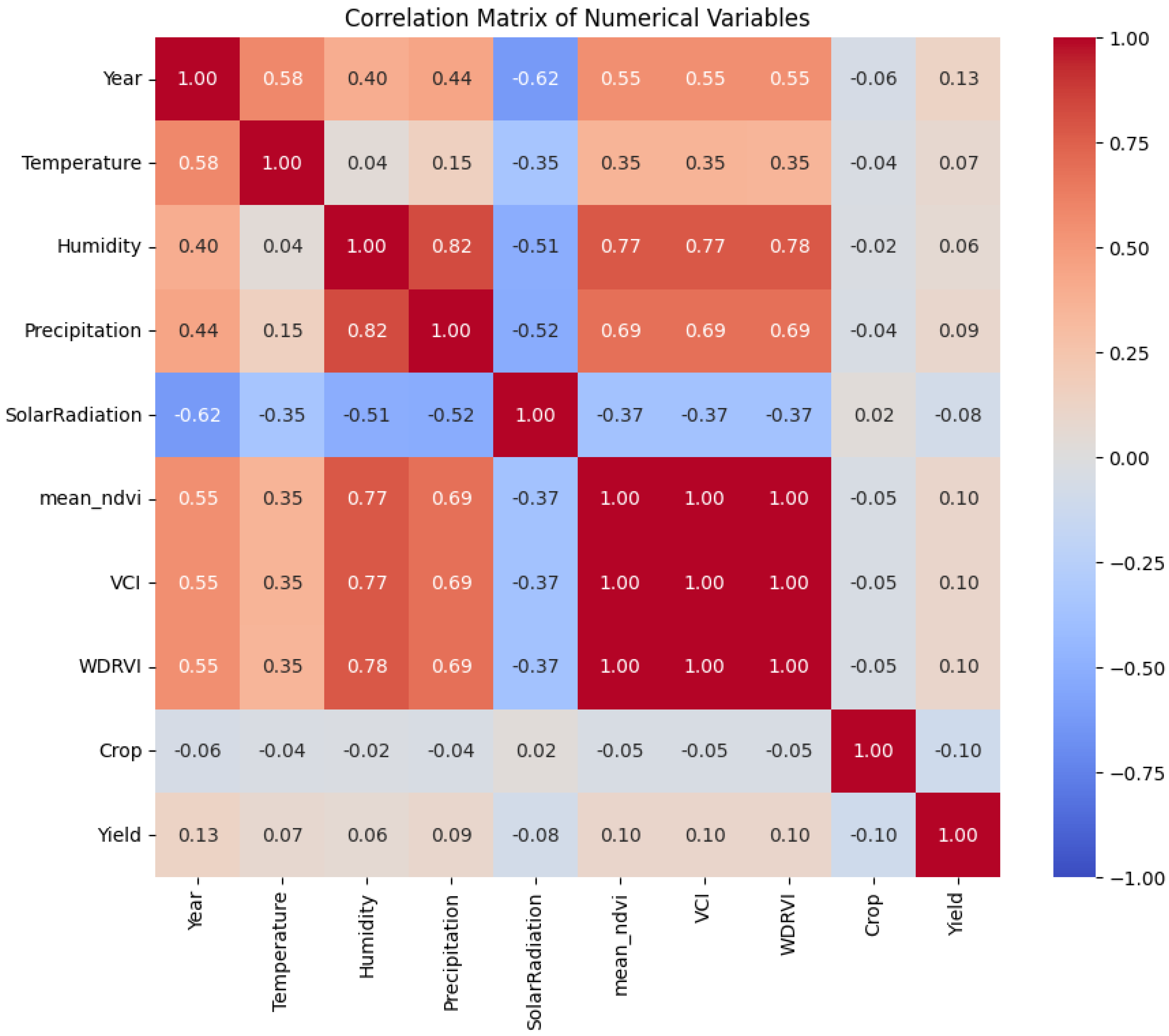
For investigating inter-feature correlations, allowing the discovery of linear relationships and possible connections, especially regarding the categorical and target features, a correlation matrix was used. The resulting correlation matrix (Figure 3), using ‘yield’ as the variable to be targeted and ‘crop’ as the encoded categorical feature, indicates that whilst climate variables such as ‘humidity’ and ‘precipitation’ have a significant positive correlation to one another (0.82) as well as with mean_ndvi (0.77 and 0.69, for each), their linear connections toward the target ‘yield’ are remarkably weak (0.06 and 0.09). In a similar way, ‘temperature’ and ‘solar radiation’ have minor Pearson’s correlations with ‘yield’ (0.07 and −0.08, respectively), as does the encoded ‘crop’ with ‘yield’ (−0.10). This widespread weak linear relationship between all features and the target highly indicates that the fundamental connections are primarily not linear or include intricate relationships that are impossible to measure by straightforward linear measurements, suggesting that advanced non-linear methods of modeling would be more successful for the yield prediction.

2.4. Independent Deep Learning Models

By automatically discovering intricate, non-linear correlations between multi-source data, including satellite imaging, weather, and soil properties, deep learning plays a crucial part in the crop yield prediction. By capturing both spatial and temporal trends, it allows for more reliable and precise yield projections than standard modeling methods. In order to select the best model for predicting the crop yield, we implemented and compared several deep learning architectures, including a Multilayer Perceptron, a Gated Recurrent Unit model, and a Convolutional Neural Network. In this sub-section, we detail the proposed architectures for these three deep learning models applied to crop yield forecasting.

2.4.1. MLP

In artificial neural networks, a Multilayer Perceptron (MLP) [15] is a core structure that is distinguished by its feedforward architecture, which consists of one input layer, one or several hidden layers, and an output layer. In the hidden and output layers, every neuron applies a non-linear activation function after performing the weighted sum of what it receives and adding a bias component. This non-linearity is essential because it allows the network to discover nuanced and complex links in data that are not possible for linear models to grasp. To reduce the difference between the net’s guesses and the real goal values, the learnable features of the network are the scaled interconnections across neurons in consecutive layers. These weights, in conjunction with the biases, are changed during the learning phase.

MLPs are widely used in many machine learning tasks because of a number of important benefits. Their main strength is their common approximate function power, implying that, considering sufficient hidden layers and neurons, they can conceptually discover any intricate, irregular operation, facilitating their simulation of intricate relationships in high-dimensional data despite the need for the specific engineering of features. Additionally, MLPs are somehow versatile to various kinds of input and are suitable for classification and regression tasks. The recognized backpropagation is a useful technique for training MLPs, enabling them to acquire knowledge from massive amounts of data and enhance their efficacy continually.

Because the variables impacting farming results are intrinsically varied and irregular, MLPs have shown to be extremely effective in crop yield forecasting. Rainfall, chemicals, and sunlight are only a few of the inputs that make up yield; these factors interact in complex manners, and their effects might differ based on certain growth phases, soil types, and historical weather patterns. These intricate relationships are adequately modeled by MLPs, which can pick up on the nuances of dependencies that are frequently missed by conventional methods of statistics. MLPs may develop more reliable and sophisticated yield predictions by gaining insights from past information covering a variety of ecological, agronomic, and leadership practices. This helps farmers render intelligent choices about the distribution of assets and handling risks, which in turn boosts productivity in agriculture and the security of nutrition.

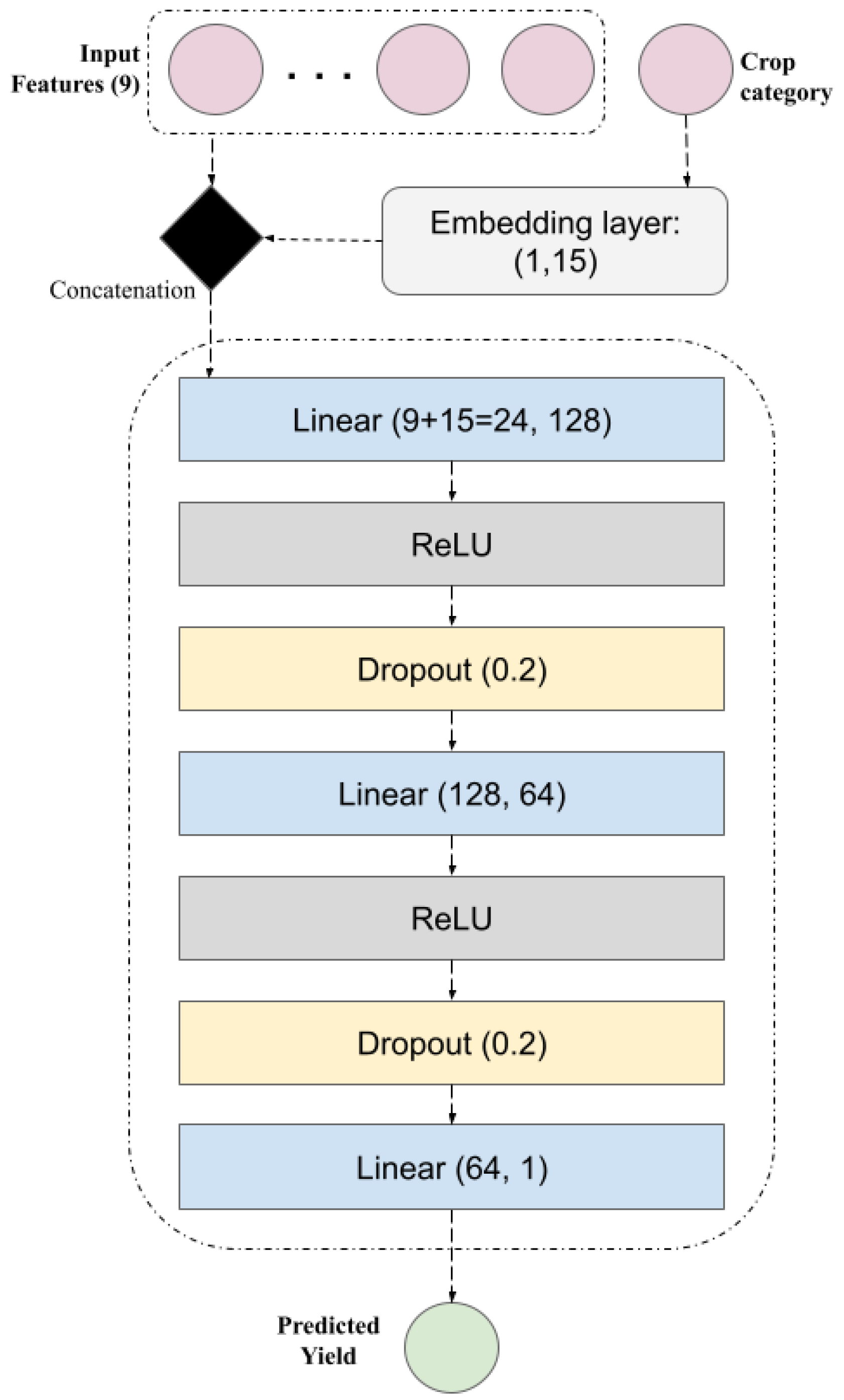
We implemented in PyTorch our MLP model for crop yield prediction, which is intended to accept a categorical depiction of the crop as input along with numerical input features (Figure 4).

A critical step is included, which is to embed the crop category into a 15-dimensional continuous vector space (the dimension of this vector space was chosen after tests with 5, 10, 15, and 20 dimensions). As a result, the model is able to discover associations between various crop varieties and how they affect the yield. The sequential fully connected network at the heart of the model has two hidden layers (128 and 64 neurons), each followed by a dropout layer to avoid overfitting and ReLU activation to introduce non-linearity. The final layer produces a single value that represents the anticipated crop production.

The crop index is initially verified to be within the acceptable range for the embedding layer by the model’s forward pass. After that, it concatenates the learnt embedding with the numerical input characteristics for the specified crop. The final prediction of yield is then generated by feeding this combined data across the layers that are fully linked. An important realization is the use of embedding for the categorical crop feature, which enables the model to learn the underlying semantic similarities across crop types in relation to yield rather than considering them as discrete tags. By reducing the chance of memorization of the training data, dropout emphasizes the importance of developing a strong and broadly applicable model.

2.4.2. GRU

A particular kind of recurrent neural network (RNN) [16] called Gated Recurrent Units (GRUs) [17] was created to manage serial input and overcome frequent problems with conventional RNNs, like vanishing gradients. GRUs regulate how information flow via the network using gating mechanisms, namely, the update gate and reset gate, which enable it to preserve pertinent historical data while eliminating irrelevant information. Because of this, GRUs are especially effective at learning correlations in data from time series, because precise forecasts depend on knowing the settings of earlier time steps.

In contrast to Long Short-Term Memory (LSTM) networks, GRUs have a simpler structure, which is one of their main advantages. Because GRUs use fewer gates and settings, they can train quickly, use less processing power, and frequently obtain comparable outcomes. Because of their simplified architecture, they are also less likely to overfit and are more effective with smaller datasets. GRUs are a good option for many sequence modeling applications, including weather forecasting, stock prediction, and agricultural monitoring, because they can still represent long-term dependencies despite their simplicity.

GRUs are particularly useful in agricultural yield prediction when modeling continuous data, such as series of weather-related parameters (e.g., temperature, humidity, and rainfall). Predicting how these fluctuations would affect crop growth and eventual output is made easier by their capacity to capture the dynamic shifts in environmental situations as time passes. GRUs are a potent tool in precision farming, where knowledge of the annual and meteorological impacts on crop growth is essential for resource allocation and choice-making. When incorporated into a predictive system, they can improve efficiency through the discovery of time-dependent correlations.

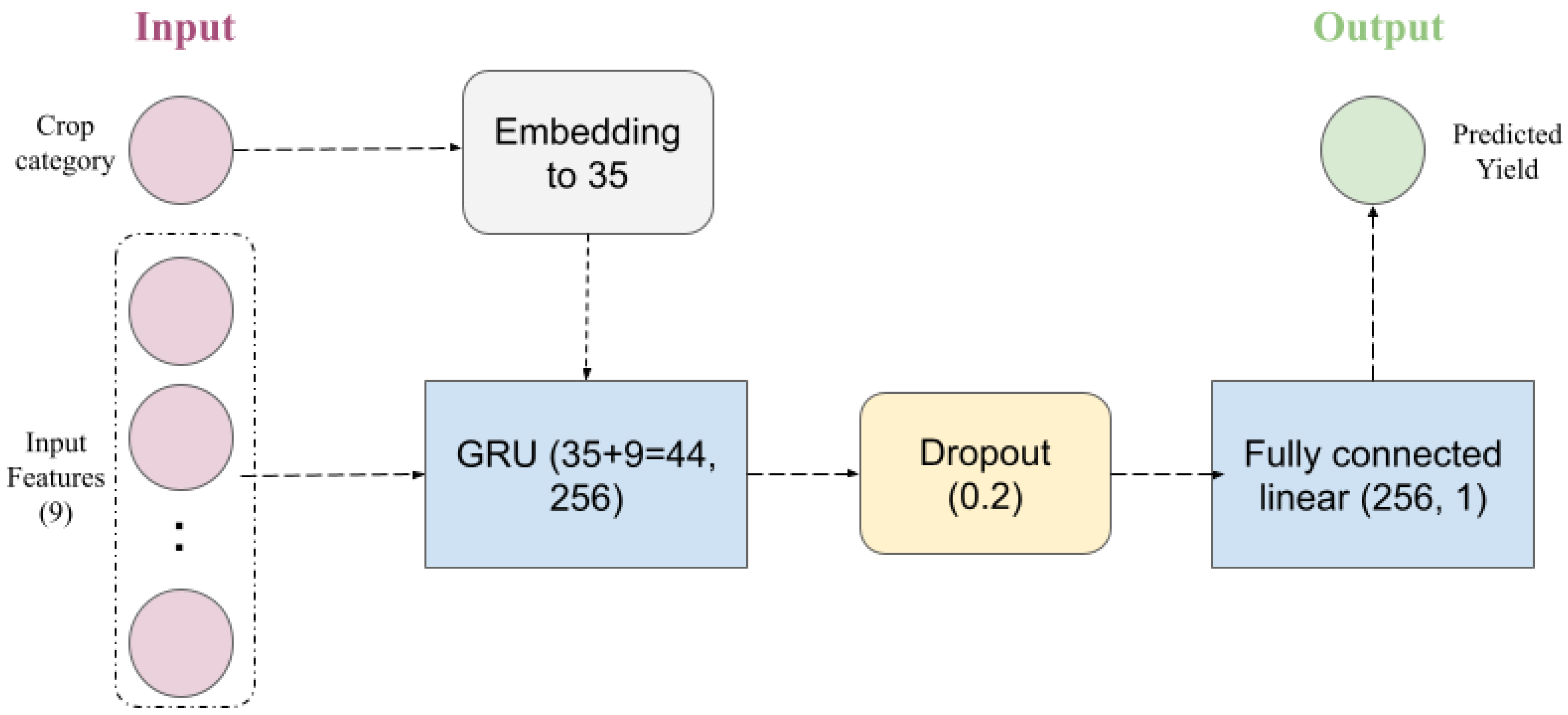
For this, we proposed the GRU architecture illustrated in Figure 5 for crop yield forecasting. The model is composed of (1) an embedding layer used to convert the crop type, which is categorical, into a 35-dimension vector; (2) a GRU layer needed to handle the sequential input (which merges the result of the embedding and the numerical features in the dataset); (3) a dropout layer for regularization; and (4) a fully connected layer for the final prediction. The embedding vector in tandem with the other parameters of the network were modified and improved according to the performance of the model. A sensitivity analysis of the embedding dimension was undertaken, ranging from 5 to 50. The embedding size of 35 was discovered to be the most beneficial for the specified objective.

2.4.3. CNN

One type of deep learning model that excels at processing data having a grid-like architecture is the Convolutional Neural Network (CNN) [18]. CNNs are made up of layers that conduct convolution tasks, which enable the neural networks to effortlessly and flexibly discover a spatial structure of aspects from the input information. CNNs are incredibly effective because each convolutional layer can identify progressively more intricate trends. CNNs have several advantages over fully connected networks, one of which is their capacity to maintain excellent performance despite lowering the number of parameters and computational expense. Weight transfer and localized interconnectivity make this occur, allowing the network to identify recurring trends and spatial correlations in input.

Because CNNs can extract useful information from satellite and aerial imagery, including plant structures, the health of crops, and properties of the soil, they are essential for predicting the production of crops. CNNs assist in identifying important temporal and spatial patterns that affect agricultural productivity by tracking these visual inputs over time. CNN-based models can produce extremely accurate yield estimates and provide insights into crop stressors when combined with weather data and other agronomic parameters. They are an essential tool for precise farming and sustainable agricultural methods because of their ability to process enormous volumes of high-resolution image data.

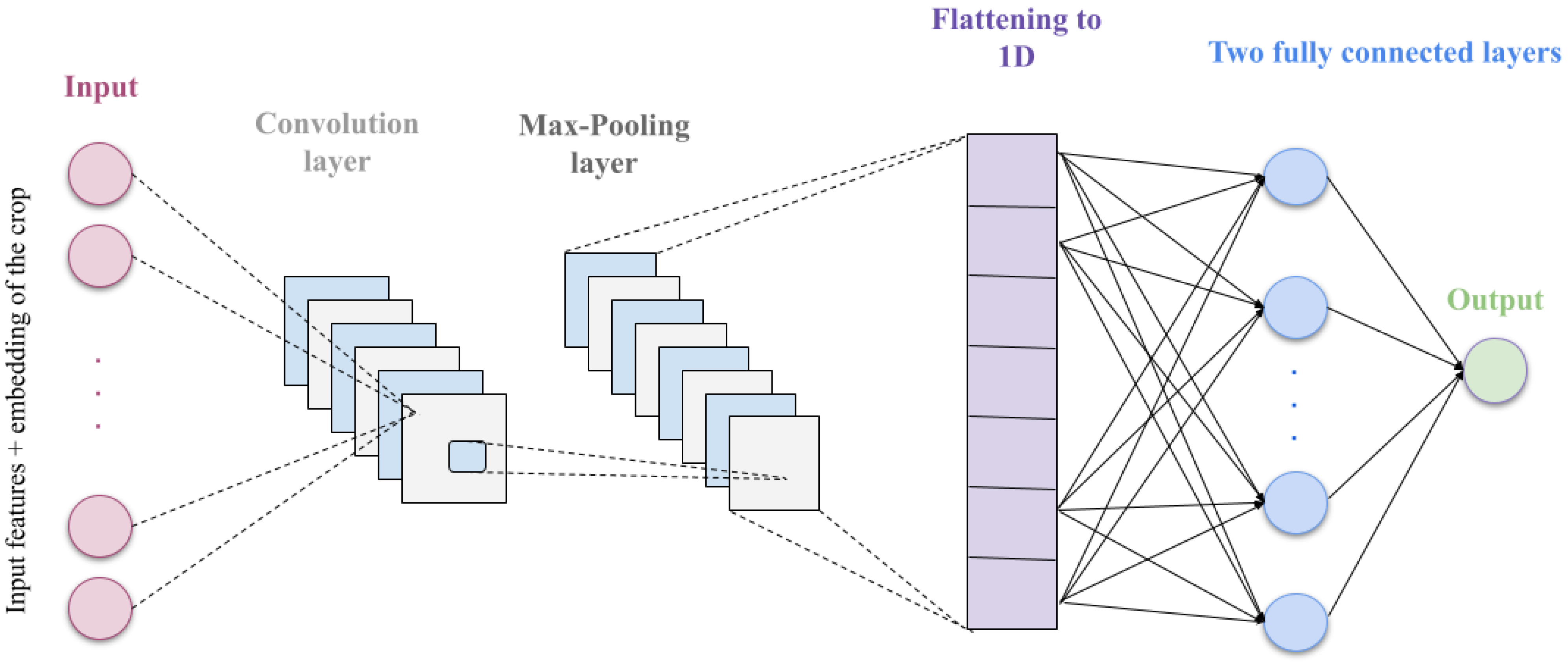
For the third deep learning model we used for the crop yield prediction, we defined a CNN model with the architecture illustrated in Figure 6. Crop types were encoded as dense vectors by the CNN model’s embedding layer (20 was the size that resulted in the best performance), followed by a combination of the input characteristics (9 numerical features). This merged data (total features of 29), a channel dimension of 1, and a batch size of 32 were subsequently passed to a 1-dimensional convolutional layer. We used 32 filters, a kernel size of 3, and a padding of 1, and then a ReLU activation function. Finally, we defined a max pooling layer (a 1-dimensional max pooling layer with a kernel size of 2). Collectively, such layers decreased the dimension of the data and extracted local patterns. With neurons’ random deactivation while training, a dropout layer was added to avoid overfitting. After that, the output generated by the pooling and convolutional layers was flattened and fed to two layers that were fully connected. Sixty-four neurons comprised the first fully linked layer, followed by a dropout for additional regularization and a ReLU activation function. One output value, which reflected the anticipated yield, was produced by the last entirely connected layer. This design unites the versatility of layers that are fully connected for the crop prediction task with the strength of feature extraction in convolutional and max-pooling layers. For sake of simplicity, we showed in Figure 6 only the input layer, the convolutional and max pooling layers, the two fully connected layers, as well as the operation of flattening the output of max pooling to 1-dimentional data to be fed to the first fully connected layer.

2.5. Ensemble Deep Learning Models

Individual models may possess varying levels of confidence or knowledge. A more accurate understanding of prediction uncertainty can be obtained through ensemble approaches [19]. Ensemble deep learning collects the findings from different deep learning models and offers an ultimate prediction that is more reliable and accurate than every one of the models in question might produce on their own. It relies on the idea that various kinds of models may improve the strengths of one another and mitigate each other’s shortcomings if their outcomes are properly combined.

On the one hand, combining various models allows the ensemble to reduce individual models’ mistakes and capture more intricate patterns in the data, increasing the prediction accuracy. On the other hand, the biases of a single model are less likely to affect the ensembles. Even if one model predicts incorrectly, the others may still do so accurately, making the total prediction more solid and trustworthy. Furthermore, by averaging out the overfitting tendencies of individual models, combining models that were trained differently can improve the generalization to unknown data.

Among the many ensemble techniques that are well explored in machine learning in general, we present in the following only the three techniques that resulted in better performance (blending, stacking, and boosting) when we applied them to the deep learning models we propose (MLP, GRU, and CNN).

• Blending is an ensemble method that improves the prediction accuracy by merging the outcomes of the baseline models. This technique builds on the capabilities of various models to produce a more resilient and precise forecasting system. Blending, rather than depending on a single model’s forecast, combines the starting model’s projections by applying a meta-learner, which may be applying linear regression (LR), support vector regression (SVR), or any traditional machine learning model (we applied LR and SVR). The mixing process consists of several critical steps, as illustrated in Figure 7. First, the data is divided into three categories: training, blending, and testing. The basis versions are trained on the training data before being used to make predictions about the blending and testing sets. These basic model predictions on the blending set are then blended to create additional features that are utilized to train the meta-learner. Finally, base model predictions from the testing set are input into the trained meta-learner, which generates the final predictions. The blended model’s performance is evaluated using measures such as R-squared, Mean Absolute Error, and Mean Squared Error, which provide information about its predictive power in comparison to individual base models.

• Stacking is a collective learning strategy that brings together the predictions of many base models by training a meta-model to learn how to integrate their outputs optimally. Unlike blending, which trains the meta-model on a separate holdout validation set, stacking employs K-fold cross-validation to create out-of-fold forecasts from the initial models used for meta-model training, thus preventing overfitting and ensuring improved generalization. In comparison, blending is simpler and faster to construct, but it may result in overfitting if the remaining set is not realistic. The meta-learner in the stacking procedure discovers the optimal way to integrate the predictions of the underlying models. We implemented a stacking ensemble that first generates mean predictions for each model across multiple forward passes, utilizing Monte Carlo Dropout (MC Dropout) for the uncertainty assessment, and then combining results from the base models (MLP, GRU, and CNN). A ridge regression meta-learner is trained to determine the best weights for mixing the outputs of the basic models using the mean predictions packed jointly as feature inputs. The final ensemble prediction is derived from the meta-learner’s predictions, and the uncertainty of the ensemble is estimated by calculating the average standard deviation of predictions made by the base models. With this, we performed ensemble learning with uncertainty awareness.
• Boosting is the process of training deep learning models one after the other, where each new model concentrates on correcting the mistakes of the models preceding it. AdaBoost and gradient boosting variations tailored for neural networks are two examples. We used AdaBoost to leverage the predictions of the three proposed models (MLP, GRU, and CNN) to obtain a more robust and accurate prediction. AdaBoost employs a boosting technique that repeatedly trains weak learners and emphasizes unpredictable data points. This continuous method of learning contributes to increasing the ensemble’s overall accuracy. We determined the normal deviation of the initial model forecasts to assess the uncertainty related to the ensemble’s predictions. This gives information about how confident the model is in its forecast for every data point. Boosting establishes models sequentially, correcting past errors, whereas stacking and blending integrate numerous models together via a meta-model.

2.6. Evaluation

After defining each of the proposed models, their accuracy, robustness, and uncertainty estimation need to be evaluated. For all the models studied, we implanted a common evaluation function that assesses the model’s efficacy. This function is intended to assess a model’s performance and measure the prediction uncertainty using the Monte Carlo Dropout technique. It returns a variety of assessment metrics, together with the predictions and their uncertainty, after receiving as inputs the trained model, testing data, and a few more variables. The encrypted categorical information is used in this function. This enhances the evaluation’s precision and resilience by allowing the model to include data on crop types in its yield forecast procedure. We used a variety of indicators to assess how well each suggested deep learning model made its prediction. The metrics used to evaluate the models’ performances were R-squared (R²), Mean Absolute Error (MAE), and Mean Squared Error (MSE) [20]. Also, we computed the Mean Prediction Interval Width (MPIW) and Prediction Interval Coverage Probability (PICP) for quantifying uncertainty. In addition, we used the Explained Variance Score for the proposed ensemble models.

• Mean Squared Error (MSE): The average of the squared variance among the real outcomes ($y_i$) and the predicted ones (${\widehat{y}}_i$) is measured by this metric. MSE highlights greater errors by squaring the errors, which makes the statistic susceptible to outliers. The outcome is a value that is simple to calculate and expresses the total size of the prediction mistakes. As the forecasts are generally nearer to the true values, a smaller MSE suggests that there is more agreement between the model and the data. Nevertheless, because the MSE values are squared in relation to the goal variable’s units, the straightforward meaning may be a little less obvious.

  $$MSE={\displaystyle \frac{1}{n}}\sum _{i=1}^n{\left(y_i-{\widehat{y}}_i\right)}^2$$

• Mean Absolute Error (MAE): This metric computes the average of the total variations among the predicted outcomes (${\widehat{\mathrm{y}}}_{\mathrm{i}}$) and the real values (${\mathrm{y}}_{\mathrm{i}}$). Because MAE does not abnormally weight big errors, it is more resilient to outliers than MSE because it handles all errors equally. The resulting value is frequently easier to read than MSE since it shows the average size of the mistakes in the same units as the target variable. In terms of relative difference, a lesser MAE means that predictions made by the model tend to correspond to reality.

  $$MAE={\displaystyle \frac{1}{n}}\sum _{i=1}^n\left|y_i-{\widehat{y}}_i\right|$$

• R-squared (R²): The coefficient of determination, or R-squared (R²), is a measure of how much variation in the variable in question can be predicted from the given variables. In essence, it indicates how well the model matches the observed data in comparison to a basic model that consistently forecasts the dependent variable’s mean ($\overline{\mathrm{y}}$). A model that reflects all the variance in the target variable has an R² score of 1, whereas one that reflects none of the variance has a value of 0. The percentage of deviation that the model describes is represented by values ranging from 0 to 1.

  $$R^2=1-{\displaystyle \frac{{\sum }_{i=1}^n{\left(y_i-{\widehat{y}}_i\right)}^2}{{\sum }_{i=1}^n{\left(y_i-\overline{y}\right)}^2}}$$

In order to deploy deep learning responsibly and safely in a very important field like crop yield prediction, it is essential to implement quantifying uncertainty [21]. This makes deep learning models more reliable and more translucent, allowing them to show when their results should be considered with suspicion. When measuring the degree of uncertainty in a model’s forecasting, the Mean Prediction Interval Width (MPIW) and Prediction Interval Coverage Probability (PICP) are especially crucial. They are essential measures for assessing the validity of prediction intervals, because they offer a range of reasonable estimates as opposed to just one prediction.

• MPIW: The average width of the prediction intervals produced by a model is measured by the MPIW. In general, a narrower MPIW is preferable since it denotes a more accurate forecast. Whether or not a model is confident, if it frequently generates large prediction intervals, these ranges are less useful for making decisions. Intervals for predictions should be as small as feasible while still accurately representing the actual values.

  $$MPIW={\displaystyle \frac{1}{n}}\sum _{i=1}^n\left(U_i-L_i\right)$$

  where ${\mathrm{U}}_{\mathrm{i}}$ and ${\mathrm{L}}_{\mathrm{i}}$ are the upper and lower bounds of the prediction interval for the ith prediction.

• PICP: It measures the percentage of the real results that fall inside the model-generated interval of prediction over a collection of forecasts. A good model ought to possess a PICP that is near the required confidence level for a prediction interval. Under confidence, indicated by a PICP that is much below the confidence level, means that the intervals are too small and do not always catch the genuine values as frequently as they should. On the other hand, overconfidence is indicated by a PICP that is noticeably above the degree of trust, wherein the gaps are broader than required and the forecasts are less accurate.

  $$PCIP={\displaystyle \frac{1}{n}}\sum _{i=1}^{n}I\left(y_i\in \left[L_i,U_i\right]\right)$$

  where $I\left(y_i\in \left[L_i,U_i\right]\right)$ equals 1 if the actual value ${\mathrm{y}}_{\mathrm{i}}$ falls within the interval, and 0 otherwise.

3. Results and Discussion

Following the methodical process described in the previous section, we present in this section the major findings of our research into deep learning for crop yield predictions in Saudi Arabia using different models and their ensembles. We will use a combination of quantitative indicators and visual aids to critically examine these findings and their relevance to the field. Then, we will discuss the uncertainty quantification performed to assess the trustworthiness and safety of the obtained predictions. Finally, we will place our results in the context of the current literature, examining points of agreement, disagreement, and possible new additions.

3.1. Performance Evaluation

To evaluate the performance of the suggested models, we applied common regression metrics: R², MSE, and MAE. Together, these metrics assess the model’s accuracy in forecasting crop yields. R² shows the percentage of yield variance that the model can account for, while MSE and MAE assess the mean amount of errors.

According to

Table 2. Comparison of the prediction performance for the proposed deep learning models: Multilayer Perceptron (MLP), Gated Recurrent Unit (GRU), and Convolutional Neural Network (CNN). The metrics used were R-squared (R²), Mean Absolute Error (MAE), and Mean Squared Error (MSE).

	MLP	GRU	CNN
R2	0.89	0.94	0.91
MAE	0.22	0.17	0.20
MSE	0.11	0.06	0.09

, the evaluation of our predictive models yielded distinct performance characteristics, as quantified by R², MAE, and MSE. Although some baseline methods surpassed the obtained R², they showed that the MAE and MSE were very high and they lacked a guarantee of reliability and trustworthiness, since no study quantifying uncertainty was performed.

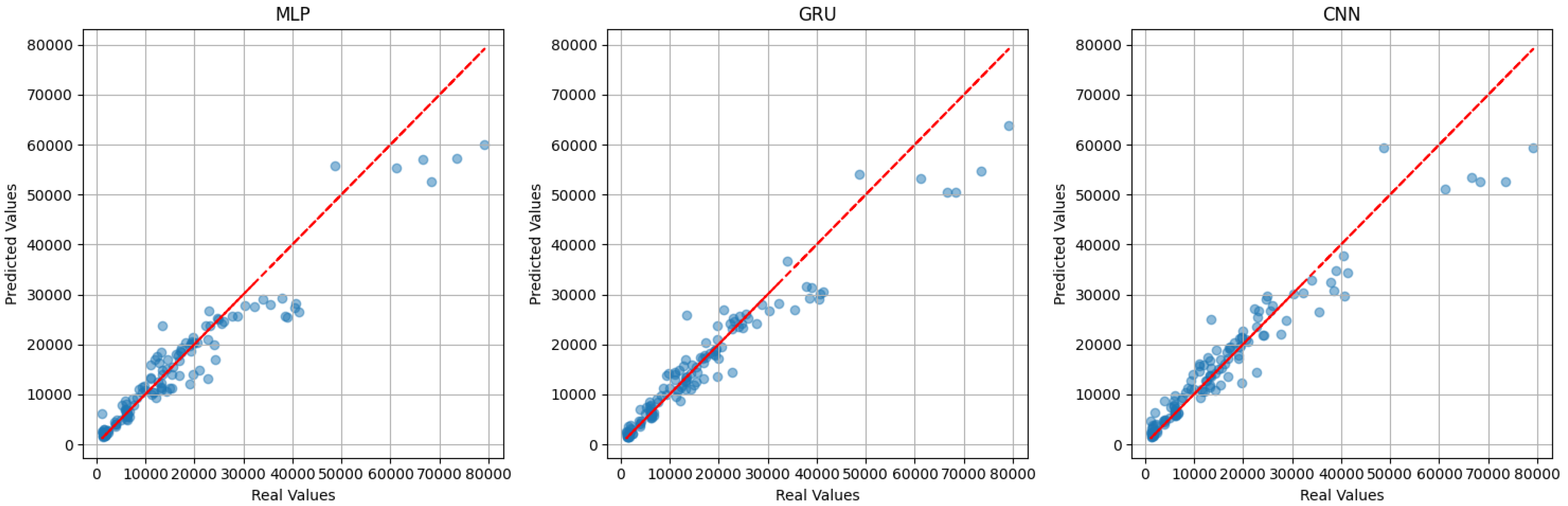
For the three proposed independent models, GRU achieved the lowest MSE of 0.06 and MAE of 0.17, indicating the smallest average magnitude of squared and absolute errors, respectively. In contrast, MLP exhibited a higher MSE of 0.11 and MAE of 0.22, which is too similar to CNN. Furthermore, the R² scores revealed that GRU explained 94% of the variance in the target variable, whereas MLP accounted for 89%, which is too similar to CNN, resulting in 91%. These initial results suggest a clear advantage of GRU in accurately predicting the target variable compared to MLP and CNN, but overall, the three models demonstrate a strong ability to explain the variability in the dependent variable. This result is also clear in the scatter plots in Figure 8, showing that for the three models, the points are more tightly clustered around the diagonal line, except some points that show that the models struggle with higher values of crop yield (greater than 65,000 kg per hectare).

To visually examine the forecasting mistakes across several result ranges, a residual analysis was carried out. For each of the three models, the distribution of prediction errors along the range of anticipated crop yields is shown by the residual plot (Figure 9). Greater dispersion is seen at higher yield values, suggesting possible variability, even though the residuals are typically centered around zero, indicating that the models represent the overall trend. This implies that the models perform better for lower yield ranges and could use variance modeling or additional refining for higher yields. The models do not exhibit systematic bias or underfitting, as further evidenced by the lack of a discernible trend in the residuals. These revelations, which are not apparent from scalar measurements such as R², highlight how crucial a residual analysis is to a reliable assessment of models.

On the other hand, when ensembling the three deep learning models, MLP, CNN, and GRU (

Table 3. Comparison of the performance predicted for the proposed ensemble deep learning models. The metrics used were R-squared (R²), Mean Absolute Error (MAE), and Mean Squared Error (MSE).

	Blending	Stacking	Boosting
R2	0.94	0.96	0.92
MAE	0.17	0.15	0.21
MSE	0.05	0.03	0.08

), the stacking technique showed a very high score of R² (0.96) compared to the blending and boosting techniques. This suggests that approximately 96% of the variance in crop yield can be explained by the stacking-based ensemble model, indicating a strong fit to the underlying data. The boosting ensemble model performed worse than one of the independent models, whereas the blending ensemble model had the same prediction as the best one of the three models. The reason may be the fact that the basic models are very powerful and capture most of the patterns in the data. Under such circumstances, it can be difficult for an ensemble to considerably improve on it, and it may even slightly decrease the performance due to the use of less accurate forecasts with an inefficient combination technique.

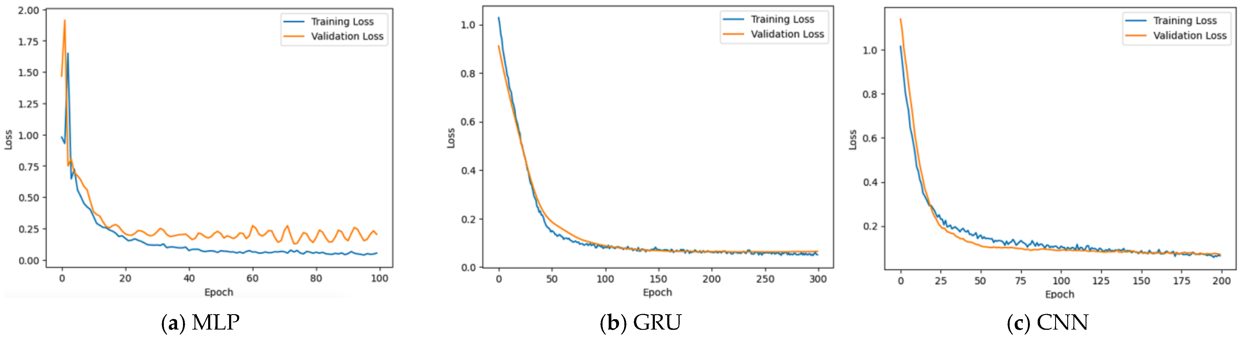
Losses during training and evaluation (or validation) serve as significant evidence of a machine learning model’s performance and learning behavior. The training loss reflects how well the model fits the training data, but the evaluation loss indicates how well the strategy generalizes to new data. Observing both losses while training aids in the detection of difficulties such as overfitting (where the training loss reduces while the validation loss increases) and underfitting (when both losses remain large). A high-performing model should have a declining trend in both losses, with the validation loss stabilizing at a low value. As a result, assessing these losses is critical for understanding the model’s learning processes, guiding hyperparameter adjustment, and assuring reliable results for data from the real world. We drew in Figure 10 plots showing the training loss (blue line) and validation loss (orange line) for the three models: MLP, GRU, and CNN. The curves indicate a better training process with good learning and generalization for both GRU and CNN compared to MLP.

Figure 10a shows that for MLP model, in the first 10–15 epochs, both training and validation losses are reduced dramatically. This shows that the model is learning efficiently and generalizing well to previously unseen validation data at this phase. Following the first quick decline, the training loss continues to fall, but more slowly, and eventually attains a lower value than the validation loss. The growing disparity between training and validation losses, together with a plateauing and mild rising trend in the validation loss, indicates that the model is beginning to overfit the training data. Although it tends to improve on previously observed data, its ability to generalize to new, unknown data deteriorates.

For the GRU model (Figure 10b), the training loss shows a smooth and significant decrease over the 200 epochs, converging to a relatively low value. The validation loss closely follows the training loss initially, also decreasing significantly. While there is a small gap, the validation loss also reaches a low value and remains relatively stable toward the end, tracking the training loss well. The gap between the training and validation losses is consistently small, especially in the later epochs.

The training vs. validation loss plot for CNN model (Figure 10c) shows a well-behaved learning process without significant overfitting. The training loss and the validation loss both decrease steadily during the first 100 epochs. The two losses remain close together throughout training, which proves that the model is generalizing well. After around epoch 150, both curves flatten out, indicating that the model has likely converged. There is no overfitting, since the validation loss does not increase while the training loss decreases.

3.2. Uncertainty Quantification

Uncertainty quantification is an important component in deep learning initiatives, especially in high-stakes areas such as agriculture, where the predictions must be credible and transparent. It allows practitioners to discern between high-certainty and high-risk forecasts, resulting in better risk management and informed judgments. It also assists in identifying areas where the model may be failing or where further data is required, making it an effective tool for iterative model improvement. Furthermore, adding an uncertainty quantification increases trust by offering not only a forecast but also an awareness of how much that prediction can be relied on. To apply an uncertainty quantification to our deep learning models for crop yield prediction, we chose to apply the MC Dropout technique. To assess the reliability and tightness of uncertainty intervals, we computed the Prediction Interval Coverage Probability (PICP) and the Mean Prediction Interval Width (MPIW) and reported some visual diagrams to help interpret the performance. Each of the three models necessitated specific techniques for hyper tuning and calibration, which contributed to reaching the promising results shown in

Table 4. Uncertainty quantification for the proposed deep learning models. The metrics used were the Prediction Interval Coverage Probability (PICP) and the Mean Prediction Interval Width (MPIW).

	MLP	CNN	GRU
PICP	0.85	0.96	0.95
MPIW	0.89	0.60	3.66

. CNN is the best performing, as it achieves high coverage (PICP = 0.96) with the smallest average interval width (MPIW = 0.6). GRU achieves good coverage but at the cost of very wide intervals (PICP = 0.95 and MPIW = 3), suggesting a high degree of uncertainty or less precise predictions. MLP resulted in a PICP = 0.85 and MPIW = 0.89, having slightly lower coverage than the others, but its interval width is also relatively narrow.

3.2.1. Enhancing the MLP Model

We used Hyperopt for hyperparameter adjustment in order to maximize the model’s performance. We established an objective function that uses five-fold cross-validation to train and assess the model with a specified set of hyperparameters, with the goal of minimizing the Mean Squared Error. For hyperparameters like learning rate, number of neurons, and dropout rate, Hyperopt searches for a predefined search space. Metrics like MSE, R², MAE, PICP, and MPIW are used to assess the final MLP model’s performance on the test set after the optimal hyperparameters have been determined. In order to manage possible variations in feature scales and the distribution of the target variable, StandardScaler was used for scaling. Finding the best model parameters is automated when Hyperopt is used for hyperparameter optimization, which increases productivity and resulted in improved model performance. The average squared difference between the predicted and actual values is the main goal of choosing MSE as the objective function. Lastly, the evaluation metrics offer a thorough analysis of the model’s uncertainty and predicted accuracy.

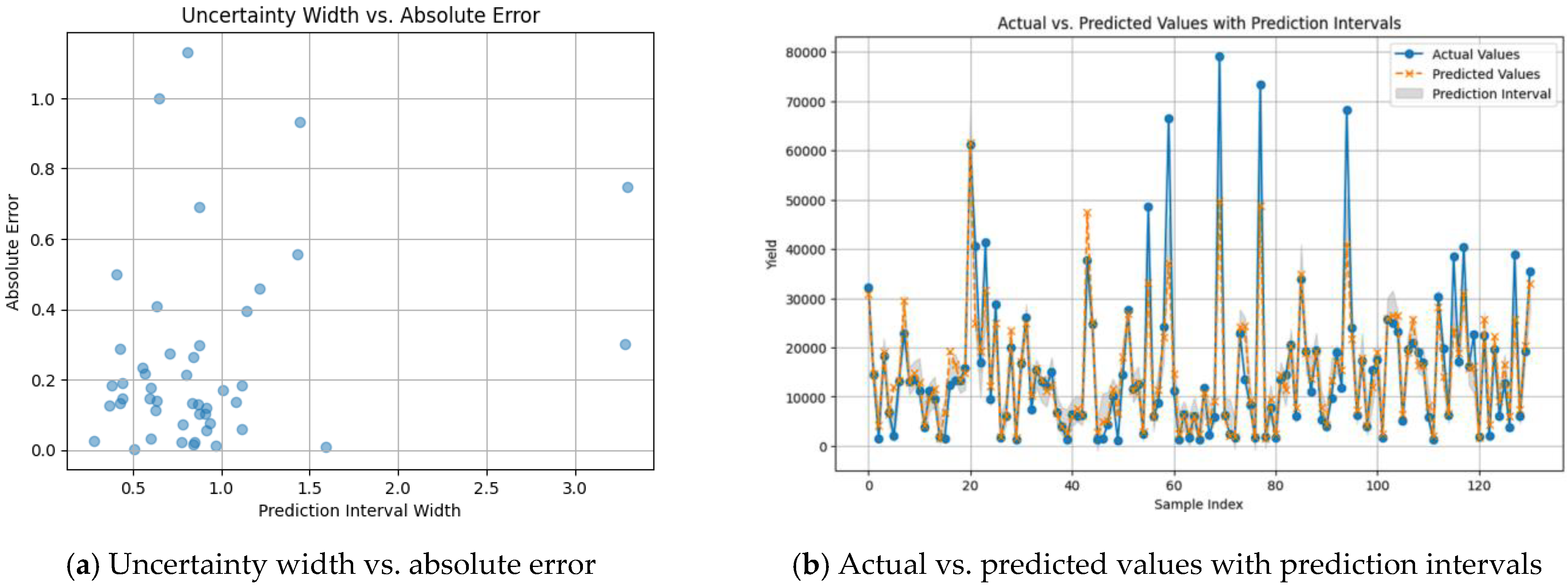
The scatter plot in Figure 11a shows a pattern that generally indicates a desirable behavior of the MLP model’s uncertainty estimation, but with some potential areas for improvement. The model demonstrates a minimal absolute error (accurate predictions) and low uncertainty (narrowed forecast range) for many predictions, as indicated by the high number of points located in the bottom left quadrant. This is encouraging because it indicates that the model is generally accurate and confident. The existence of specific upward and leftward trending points indicates that the absolute error tends to rise in parallel with uncertainty. The model is generally aware whenever it is more probable to be incorrect and conveys it through broader prediction intervals, which is the appropriate beneficial correlation we would like to observe. The existence of two data points with large prediction intervals (around 3.2) coupled with relatively low errors suggest that the model’s uncertainty quantification may be improved with more examination of these opposing scenarios, which may also provide strategies for increasing accuracy even in the face of high uncertainty.

On the other hand, Figure 11b shows a comparison between actual crop yield values (in blue) and the predicted values (in orange) made by MLP model, along with the uncertainty bounds (prediction intervals shaded in gray). This confirms good model performance since the predicted values follow the trend of the actual values. Moreover, the range of the prediction intervals varies (wider where the model is less confident), which suggests an adaptive uncertainty estimation, showing the strength of MC Dropout. However, in some cases, the actual values lie outside the gray-shaded area, these are the prediction failures that lead to a PICP of 0.85, as shown in Table 4.

3.2.2. Enhancing the GRU Model

This model uses an embedding layer to represent various crops, a bidirectional GRU layer to identify temporal connections, batch normalization to stabilize training, and dropout to regularize. To improve the prediction’s trustworthiness, the model incorporates Monte Carlo (MC) Dropout during the evaluation, which creates numerous forecasts for each input to approximate uncertainty. This uncertainty is then utilized to provide prediction intervals that indicate a range where the real crop yield is expected to fall, as well as metrics such as PICP and MPIW. Beyond basic model construction and uncertainty calculation, the model emphasizes consistency by using random seeding. It employs the Adam optimizer to customize the weights of models and gradient clipping to avoid overflowing gradients. Isotonic regression is used to adjust the model’s predictions to better align with the true distribution of the target variable, thus improving the calibration of the uncertainty estimates.

Based on the best methods and strategies utilized in our model, scaling ought to have a favorable impact on the uncertainty quantification process. Scaling helps to improve the model’s general efficiency and calibration, resulting in more trustworthy uncertainty estimations and prediction intervals. In our model, we chose to use a scaling factor of 1.25 since it offers the optimal balance among usefulness and coverage. An example of varying the model parameters is reported in

Table 5. Reporting the Prediction Interval Coverage Probability (PICP) and the Mean Prediction Interval Width (MPIW) while changing the scaling factor.

	Scaling Factor
	1	1.25	1.5	1.75	2.5
PICP	0.88	0.95	0.97	1	1
MPIW	3.84	4.84	5.81	6.78	9.69

.

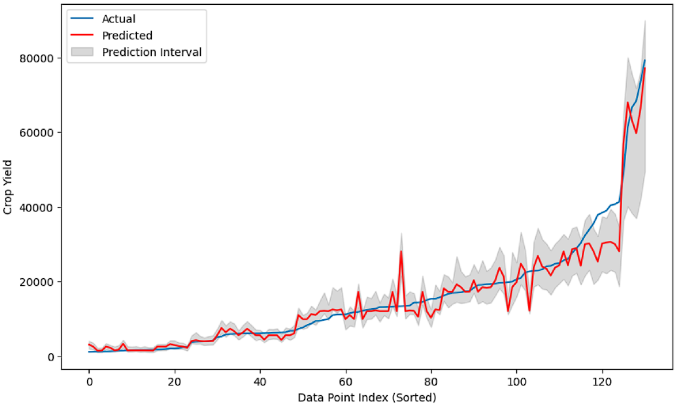
To gain a thorough understanding of the model’s reliability and efficacy, plotting actual vs. expected crop production with prediction intervals is critical. Prediction intervals express uncertainty, providing insights into how much faith may be placed in each forecast. This is particularly crucial in agriculture, because decisions made according to overly confident or uncertain models can have serious economic and environmental consequences. Figure 12 plots the actual vs. predicted crop yields with prediction intervals. The red “Predicted” line generally follows the same trend as the blue “Actual” line, demonstrating that the model catches some of the underlying trends in crop production data. The gray-shaded area illustrates the model’s confidence in its forecasts. The width of the prediction interval varies with the data points. In some areas, the range is quite narrow, indicating greater confidence. In other areas, especially when the yield fluctuates quickly or reaches higher levels, the interval expands, indicating higher levels of uncertainty.

3.2.3. Enhancing the CNN Model

Accurate crop yield forecasts are critical, but comprehending the uncertainty related to those predictions is essential. This is where MC Dropout steps in. MC Dropout generates a spread of forecasts rather than one point estimation by executing the model using various dropout masks on multiple occasions throughout the inference. This distribution reflects the model’s forecast uncertainty, permitting forecast intervals—ranges in which the true output is probable to fall—to be calculated. This is useful for risk estimation and making decisions in agriculture, since it provides an additional view of the possible outcomes. MC Dropout produces a distribution of predictions, which helps to better reflect the model’s genuine uncertainty, resulting in more trustworthy prediction intervals and probability estimations. By quantifying uncertainty, MC Dropout assists in understanding the risks associated with various crop management practices and, ultimately, making educated decisions. This algorithm assesses the accuracy of uncertainty estimates and calibration using measures such as PICP and MPIW, ensuring that the prediction ranges are relevant and reliable. MC Dropout for the CNN entails keeping dropout active during inference, performing numerous forward moves resulting in a distribution of forecasts, and employing this distribution to determine uncertainty and identify prediction intervals, which makes the model’s forecasts more useful and reliable for practical use. We used K-Fold cross-validation to train and evaluate the model on different subsets of the data, which helps to obtain a more robust estimate of the model’s performance. Throughout the evaluation stage, dropout is usually switched off. To use MC Dropout, we purposefully keep it active during inference. This is performed implicitly in PyTorch 2.6 by switching the model into training mode prior to making predictions. To obtain a prediction distribution, the model is run many times using the same input data but different arbitrary dropout masks at each pass. We store the results of all forward passes and determine the average forecast over these samples. This average serves as a point estimate for the prediction. By including K-fold cross-validation, the code intends to create a more robust CNN model for forecasting crop yields that generalizes better to new data and delivers more accurate uncertainty assessments. After different experimentations, the number of folds chosen was 15.

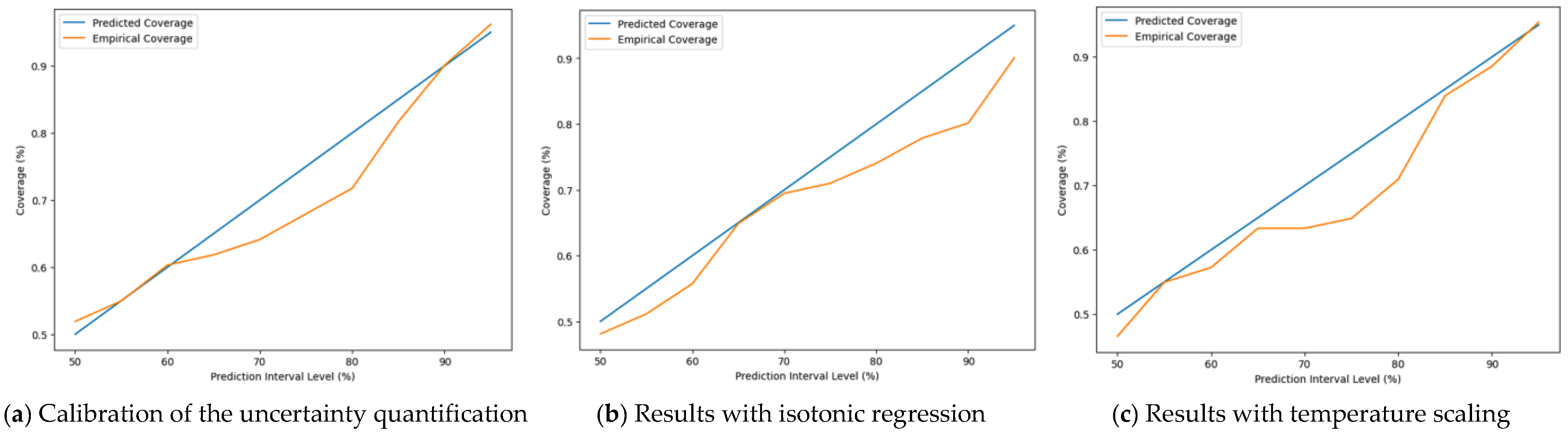
To measure how well the CNN model’s projected uncertainty corresponds to actual outcomes, we referred to the projected vs. empirical coverage charts, often known as reliability diagrams. These diagrams aid in evaluating the prediction interval calibration, as the experimental coverage should nearly match expected interval values, indicating accurate uncertainty estimations. The reliability diagram drawn in Figure 13a visualizes the calibration of uncertainty quantification for our CNN model. The blue line shows a perfect calibration, meaning that the predicted confidence matches the empirical coverage exactly. However, the model tends to be overconfident (orange line), particularly in the mid-range (60–80% intervals). This implies that the uncertainty estimates of the model might need calibration.

To overcome this issue, we used isotonic regression, which led to the plot in Figure 13b. The blue diagonal line depicts perfect calibration, which occurs when the projected and empirical coverages coincide perfectly. The orange line (empirical coverage) regularly goes below the diagonal, showing that the model is overconfident, with narrower prediction ranges that capture fewer true values than expected. So, the calibration via isotonic regression here did not improve the uncertainty estimates of the model.

We also implemented a calibration via temperature scaling. The result obtained in Figure 13c shows that there are still areas of miscalibration, with the model being under-confident at lower prediction interval levels (in the range of 50% to 70%) and overconfident at higher levels (above 80%). This residual miscalibration could be attributed to temperature scaling’s intrinsic limits in dealing with more complex miscalibration patterns, or to a discrepancy between our calibration and test datasets. Future research could look into more adaptable calibration approaches or changes to the basic model’s architecture.

It is also likely that the continual miscalibration found in our model, despite the use of approaches such as isotonic regression and temperature scaling, indicates that data restrictions in our calibration set are a substantial contributing factor. This data’s limited size or poor diversity most likely hindered the calibration methods’ potential to acquire a reliable and adaptable mapping among the model’s estimations of uncertainty and true probabilities or coverage.

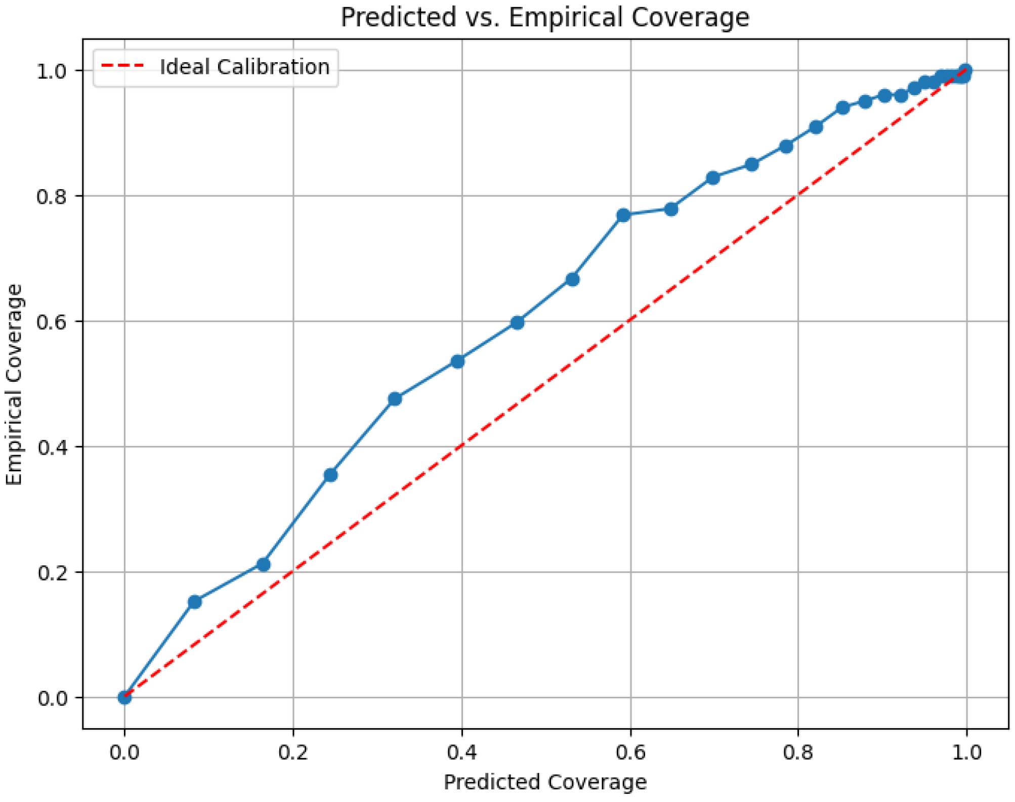
Compared to the above calibration for CNN model, the predicted vs. empirical coverage for the blending-based ensemble model, for example, (Figure 14) showed a reasonable calibration, a slight underconfidence at moderate prediction intervals, yet a well-calibration at high confidence levels. The blue curve is mostly above the red line between 0.3 and 0.7, and it suggests that the model is slightly underconfident in that range, meaning that it is being cautious and its prediction intervals are a bit wider than necessary. However, at higher coverages (after 0.7), the curve gets closer to the ideal line, indicating better calibration at higher confidence levels.

3.3. Comparison to Existing Approaches

Crop production forecasting in Saudi Arabia has used a variety of methodologies, involving statistical techniques, satellite imagery, and artificial intelligence algorithms [4,22,23,24,25,26,27,28,29]. Classical statistical approaches, such as regression, offer foundation forecasts but frequently do not account for the intricate relationships among environmental variables. Remote sensing methods, especially satellite imaging, are being used to track crop quality and predict yields across wide areas. For example, indices developed from satellite data, such as the Normalized Difference vegetative Index (NDVI), have demonstrated promising results in measuring vegetative health and forecasting yields.

By incorporating various sources of data, which include weather information, soil characteristics, and remote sensing indicators, machine learning methods like Random Forest (RF), Support Vector Machine (SVM), and deep learning models have enhanced precision when estimating crop yields [23,26,27,28].

In [26], the authors obtained for the k-nearest neighbors (KNNs), Decision Tree (DT) regressor, Bagging regressor, RF regressor, and eXtreme Gradient Boosting ensemble (XGB) a score R² between 0.95 and 0.97, but the metrics related to the Root Mean Square Error (RMSE) and Mean Absolute Error (MAE) were high, which show an increasing amount of errors. They concluded that the ensemble method surpassed each of the independent techniques for crop type detection.

Considering only the temperature, insecticides, rainfall, and crop yields for potatoes, rice, sorghum, and wheat, the authors of [27] showed that artificial neural networks performed well, with an R² between 0.90 and 0.99.

In [28], the authors used rainfall, temperature, and yield to propose a maize yield prediction framework for Saudi Arabia by a Multilayer Perceptron using Spider Monkey Optimization. The model outperformed XGB, RF, and SVM, achieving an R² of 0.98.

The work in [23] proposed a neural network model to predict crop yields across Gulf countries, achieving an R² of 0.93 by leveraging key features like temperature, rainfall, nitrogen, and pesticide use.

While the existing works focused on varying the data sources and trying different machine learning and deep learning models, they lack a guarantee of reliability and trustworthiness since no study of uncertainty quantification is performed. Also, no research has addressed different deep learning models, and ensemble deep learning has not been investigated. We believe that this research is the first to study the uncertainty quantification for the proposed models to guarantee that the obtained prediction is reliable.

4. Conclusions

Forecasting agricultural yields is an important area of research, motivated by the pressing need to provide food safety, economic security, and the long-term management of resources in the face of population expansion and climate change [30,31,32,33]. Traditional approaches and older prediction models frequently fail to capture the complexity of farming systems, resulting in inefficiency and environmental pressure. Deep learning is a powerful alternative capable of detecting subtle patterns across enormous and diverse datasets, such as those derived from remote sensing and Internet of Things technology [24,34]. Deep learning allows a move toward proactive, data-informed agriculture by providing accurate forecasts for the yield estimation and resource allocation, thus increasing food system effectiveness, sustainability, and robustness.

Based on the crucial need for enhanced agricultural forecasting and the established potential of deep learning, this research suggests a novel way to improve the crop output prediction. It offers a reliable solution for crop production forecasting in Saudi Arabia by integrating appropriate techniques for uncertainty-aware prediction. It addresses the difficulties of agriculture in arid and resource-constrained areas by facilitating more data-efficient learning, interpretable forecasts, and risk-aware decision-making. By collecting and exploring spatiotemporal data from different sources, we created three deep learning-based solutions to crop production prediction that include an uncertainty quantification via different techniques such as MC Dropout and K-Fold cross-validation. The three models consist of a Multilayer Perceptron (MLP), a Gated Recurrent Unit (GRU), and a Convolutional Neural Network (CNN). After defining, training, and evaluating these models, they were combined via three kinds of ensemble techniques (blending, stacking, and boosting) to explore more improvement possibilities. The different proposed models (independent and ensemble-based) performed well, with a high predicted accuracy and useful uncertainty estimates, which are critical for agricultural decision-making. The best performance was achieved with the stacking-based ensemble model resulting in R² = 0.96, MAE = 0.15, and MSE = 0.03. When quantifying uncertainty, the model that showed a good quality of prediction was CNN, which resulted in maximizing the PICP to the desired confidence level while simultaneously minimizing the MPIW (PICP = 0.96 and MPIW = 0.60).

With a special focus on the trust and reliability of the proposed models, this work contributes to the expanding convergence of AI and sustainable agriculture, with a particular focus on dry countries like Saudi Arabia. This study’s findings highlight the model’s capacity to forecast yields under adverse scenarios, enabling farmers and traders to make smarter decisions about crop sales and input purchases. It also significantly improves the early detection of agricultural stress. By integrating deep learning with uncertainty quantification, this approach ensures reliable, data-driven decisions, ultimately fostering sustainable farming, reducing waste, and strengthening food security in regions facing water scarcity and climate vulnerability. Crucially, the methodology established here is intended to be reusable and versatile, with substantial potential for use and effects on various agricultural regions across the world experiencing comparable ecological and resource constraints.

While the results are encouraging, more improvements could be made by investigating domain adaptation to improve generalizability across different regions in Saudi Arabia. Moreover, concentrating on some particular crops may foster more personalized modeling, which may lead to improved accuracy in forecasting and better resource management that is matched with the crop’s unique development cycles and requirements.

To summarize, agricultural output forecasting is a critical area of research with significant implications for global food security, economic stability, sustainable development, and climate resilience. The ability to reliably predict crop yields provides stakeholders with crucial information for strategic planning and decision-making, resulting in a more productive, efficient, and resilient agricultural sector.