Article

Evaluation of Deep Learning Models for Predicting the Concentration of Air Pollutants in Urban Environments

by
Edgar Tello-Leal
1,*,†,
Ulises Manuel Ramirez-Alcocer
2,†,
Bárbara A. Macías-Hernández
1 and
Jaciel David Hernandez-Resendiz
2
1
Faculty of Engineering and Science, Autonomous University of Tamaulipas, Victoria 87000, Mexico
2
Multidisciplinary Academic Unit Reynosa-Rodhe, Autonomous University of Tamaulipas, Reynosa 88779, Mexico
*
Author to whom correspondence should be addressed.
These authors contributed equally to this work.
Sustainability 2024, 16(16), 7062; https://doi.org/10.3390/su16167062
Submission received: 12 July 2024 / Revised: 6 August 2024 / Accepted: 15 August 2024 / Published: 17 August 2024
(This article belongs to the Special Issue Changes in Atmospheric Environment)

Abstract

Air pollution is an issue of great concern globally due to the risks to the health of humanity, animals, and ecosystems. On the one hand, air quality monitoring systems allow for determining the concentration level of air pollutants and health risks through an air quality index (AQI). On the other hand, accurate future predictions of air pollutant concentration levels can provide valuable information for data-driven decision-making to reduce health risks from short- and long-term exposure when indicators exceed permissible limits. In this paper, five deep learning architectures are evaluated to predict the concentration of particulate matter pollutants (in their fractions PM2.5 and PM10) and carbon monoxide (CO) in consecutive hours. The proposed prediction models are based on recurrent neural networks (RNNs), long short-term memory (LSTM), vanilla LSTM, Stacked LSTM, Bi-LSTM, and encoder–decoder LSTM networks. Moreover, a methodology is presented to guide the construction of the prediction model, encompassing raw data processing, model design and optimization, and neural network training, testing, and evaluation. The results underscore the precision and reliability of the Stacked LSTM model in predicting the hourly concentration level for PM2.5, with an RMSE of 3.4538 μg/m3. Similarly, the encoder–decoder LSTM model accurately predicts the concentration level for PM10 and CO, with an RMSE of 3.2606 μg/m3 and 2.1510 ppm, respectively. These evaluations, with their minimal differences in error metrics and coefficient of determination, validate the effectiveness and superiority of the deep learning models over other reference models, instilling confidence in their potential.

1. Introduction

Actions that address sustainable air pollution management intend to improve the control and reduction in polluting emissions and collaborate to achieve several of the sustainable development goals promoted by the United Nations organization. In this sense, forecasting the concentration of air pollutants during highly polluted periods is an essential requirement in environmental management. Through accurate prediction models, a positive impact can be achieved on actions for the health care of the population through timely decision-making to prevent exposure to high concentration levels of air pollutants. Outdoor air pollution is a significant public health issue because of its harmful effects on humans. Air pollution is a complex mixture that includes particles, chemical substances, and biological materials. It mainly consists of particulate matter (PM2.5 and PM10), Ozone (O3), volatile organic compounds, nitrogen dioxide (NO2), carbon monoxide (CO), sulfur dioxide (SO2), and lead (Pb) [1]. The pollutants O3, PM2.5 (fine particulate matter), and NO2 have been identified as causing mortality when prolonged exposure occurs [2,3]. Long-term exposure to pollutants PM2.5 and PM10 has been correlated with chronic cerebrovascular, lung, cardiac, pneumonia, lung, cancer, and respiratory illnesses [1,4,5]. On the other hand, CO is mainly produced by industrial emissions and incomplete combustion in vehicle engines, natural gas equipment, burning wood, and fossil fuels [6]. Scientific studies have revealed significant effects on human health from exposure to CO, including myocardial ischemia, cardiac arrhythmia, and even asphyxiation or death at high concentrations [7,8,9]. Moreover, research has also linked CO exposure in pregnant women to fetal thrombosis, stillbirth, premature birth, and, in some cases, congenital heart disease [10,11,12,13].
Traditional air quality monitoring systems or information systems based on Internet of Things (IoT) technologies allow for the real-time acquisition of air quality indicators, an essential requirement for air pollution management. Therefore, these systems can support data-driven decisions to protect humans from adverse health impacts when a specific air pollutant or air quality index (AQI) exceeds permissible limits [14]. Accordingly, developing prediction models for the concentration of air pollutants allows us to anticipate the pollutant trend for the next few hours or days, aiding in the decision-making of environmental management to reduce risks and prevent human exposure to high-concentration environmental pollution. The next stage in air quality systems is the development of prediction air pollution systems for the hourly or daily concentration of air pollutants, with a high level of precision and reliability, which would be an excellent advantage for governments or agencies, supporting appropriate decision-making to safeguard human health in times of environmental contingency [15,16].
In this way, concentration levels of air pollutants (for example, PM2.5 or PM10) can be represented as time series data, that is, a sequence of observations at time intervals (hourly, 8-hour average, or daily, depending on the standard that regulates the air pollutant and the analysis that needs to be carried out), within which linear or non-linear components and the behavior within the time series data can be identified, whether they are trend, cyclical, seasonal, or irregular. The time series representing the concentration values of air pollutants have random characteristics, and the data can be linear, non-linear, or not normally distributed. Therefore, pattern identification of these data is a complex task. This behavior of the air pollutant data can be related to the natural sources that characterize the study area and the anthropogenic sources of air pollution caused by human activities.
Deep learning architectures have proven their mettle in enhancing the discriminative function of inference models in complex time series data. Recurrent neural networks (RNNs) are a key component of these architectures, and they are known for their highly efficient prediction models with time series data. RNN uses a sequence of input data with cyclic connections between blocks, where neurons are interconnected in the same hidden layer, repeatedly applying a training function to the hidden states [17]. In particular, long short-term memory (LSTM) neural networks, a variation of RNN, have shown remarkable capabilities in learning long-term dependencies, a crucial aspect of sequential data. They also effectively tackle the challenges of non-linearity, periodicity, seasonality, and sequential dependence between data sequences, as seen in air pollutant concentration levels. LSTM models have been applied to sequence and time series prediction problems in different domains [18,19,20,21] and in predicting air pollutants [22,23,24,25] and meteorological factors.
Architectural variations in LSTM architectures can influence the model performance for predicting air pollutant concentration levels, so it is important to evaluate and compare LSTM architectures using the same implementation methodology and the same partitions of the real dataset for both training and testing stages of the prediction model to identify the best prediction model. Therefore, this paper evaluates the recurrent neural networks (RNNs), long short-term memory (LSTM), vanilla LSTM, Stacked LSTM, Bi-LSTM, and encoder–decoder LSTM deep learning algorithms to predict the hourly concentration level of air pollutants PM2.5, PM10, and CO. The choice of these architectures was based on their proven effectiveness in time series prediction tasks, which is crucial for air quality forecasting. Furthermore, we propose a methodology that allows us to guide the preprocessing and preparation of the data, the design and selection of the neural network model, and the training and testing of the prediction model for each deep learning algorithm. Likewise, in the model design phase, a procedure was defined for the optimization of the hyperparameters of the neural network using the grid search algorithm to enable the selection of the prediction model with the best performance. We use root mean square error (RMSE) as a performance metric to assess the effectiveness of the prediction models.
The manuscript is organized as follows: Section 2 provides a detailed review of the related work, Section 3 presents the methodology proposed for the experimentation, Section 4 shows the results reached for each prediction model, Section 5 presents the discussion and examines its implications, and finally, Section 6 presents the conclusions and future work.

2. Related Work

In [22], the authors propose an aggregative LSTM model that combines the data from the local air quality monitoring station, the station in nearby industrial areas, and the station for external pollution sources to improve the accuracy of 1–8 h PM2.5 concentration prediction, outperforming the performance of LSTM, SVR, and gradient boosted tree regression (GBTR)-based models. Similarly, in [26], they presented a study to compare the performance of LSTM, GRU, and Bi-LSTM models in predicting hourly PM2.5 concentration using historical air pollutant data from Seoul, Daejeon, and Busan, Korea. In short-term PM2.5 prediction, all three models obtain an R2 of around 0.9; in long-term predictions, the Bi-LSTM model obtains the best performance with an R2 of 0.6. In [27], the authors evaluate the LSTM, RNN, and GRU algorithms to predict hourly PM2.5 concentrations using large five-year datasets with attributes of six air pollutants and four meteorological factors in the Istanbul metropolitan area. The LSTM+LSTM model demonstrates its high capacity, reaching an R2 of 0.97. In [28], a two-stage, semi-supervised model composed of the empirical modal decomposition (EMD) method and Bi-LSTM neural network predicts PM2.5 concentrations with very high performance according to the achieved R2 value. The EMD method allows the data to be decomposed and the frequency and amplitude features to be extracted for further input into the Bi-LSTM network. The study presented in [15] examines the performances between PM2.5 concentration prediction models based on LSTM, Bi-LSTM, GRU, Bi-GRU, CNN, and CNN-LSTM, reporting that the hybrid multivariate model allows for the achievement of more accurate concentration predictions.
Predicting concentration levels in the atmosphere of O3 and PM2.5 using a hybrid model combining a convolutional neural network (CNN) and an LSTM, strengthened with an attention mechanism, was proposed in [29]. This model outperforms the performance achieved by machine learning models such as random forests (RFs) and support vector regression (SVR), with at least 20% in the coefficient of determination (R2). Similarly, in [30], the authors propose a CNN-LSTM model to predict the hourly concentration of different air pollutants in three cities considering spatiotemporal characteristics, evaluating the performance of the model by applying two methods on the input variables that differ in using only pollutant data or pollutant and meteorological factors. In predicting the PM10 concentration, the model obtained very low values (around 0.07 μg/m3) in the RMSE metric in the three case studies, with a minimal difference when meteorological data were used. Meanwhile, in [31], they proposed two hybrid models based on CNN-LSTM and CNN–gate recurrent unit (GRU) to predict hourly PM10 and PM2.5 concentrations at 39 monitoring stations in Seoul, Korea, for the next 7 days. The CNN–GRU model better predicted PM10 concentration, and the CNN–LSTM model was better at predicting PM2.5 concentration for all monitoring stations.
In [32], a spatiotemporal graph neural network (GNN) based on the GraphSAGE paradigm to forecast O3 concentration was proposed. The model was configured for different future forecast horizons (1, 3, and 6 h). The model obtains very good performance in 1-hour predictions, and the 3-hour and 6-hour cases require the information available from all monitoring stations available in the study to maintain an acceptable RMSE and R2 value. Several novel GNN-based approaches have been proposed to exploit spatiotemporal features and dependencies in the data to improve the performance of prediction models on air pollutant concentration levels [33,34,35,36,37] and the air quality index (AQI) [38].
On the other hand, remote monitoring-based approaches have advantages over traditional methods but at a higher computational cost. The authors in [39] propose a deep learning model considering spatiotemporal features to improve the predictive accuracy of satellite-based PM2.5 measurements. Different input data such as top-of-atmosphere (TOA) and aerosol optical depth (AOD)-based measurements, with or without meteorological data, and spatial resolutions of 10 km, 3 km, and 250 m were used to evaluate the prediction model. The prediction model with TOA data achieved the best performance with an R2 of 0.70, 0.66, and 0.62 for PM2.5 predictions at spatial resolutions of 10 km, 3 km, and 250 m. The authors in [40] show an ensemble model consisting of XGBoost, Light GBM, and a linear regression method to estimate monthly PM2.5 concentration using TOA satellite data, meteorological data, and ground-level PM2.5 concentration levels to train the model, obtaining an R2 of 0.80 and RMSE of 7.07. Furthermore, in [41], an approach that uses remote monitoring with TOA data to estimate ground-level PM10 and PM2.5 concentrations every 5 min was presented. This model implements an XGBoost algorithm that achieved values of 0.89 and 0.90 in the R2 metric for the prediction of PM2.5 and PM2.5 concentrations, respectively.

3. Materials and Methods
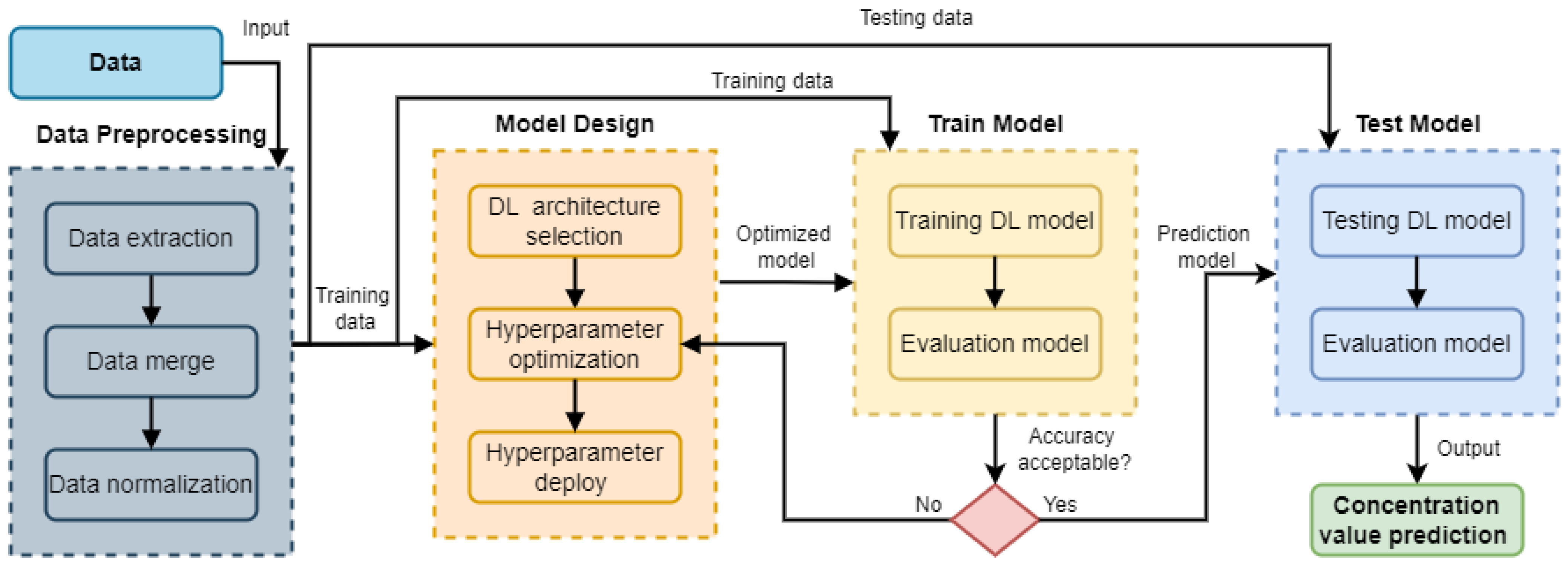
3.1. Methodology

The methodology for predicting the next hourly concentration of atmospheric pollution (PM2.5, PM10, or CO) comprisesdata pre-processing, model design, train model, andtest model phases, as shown in Figure 1.

3.1.1. Data Preprocessing
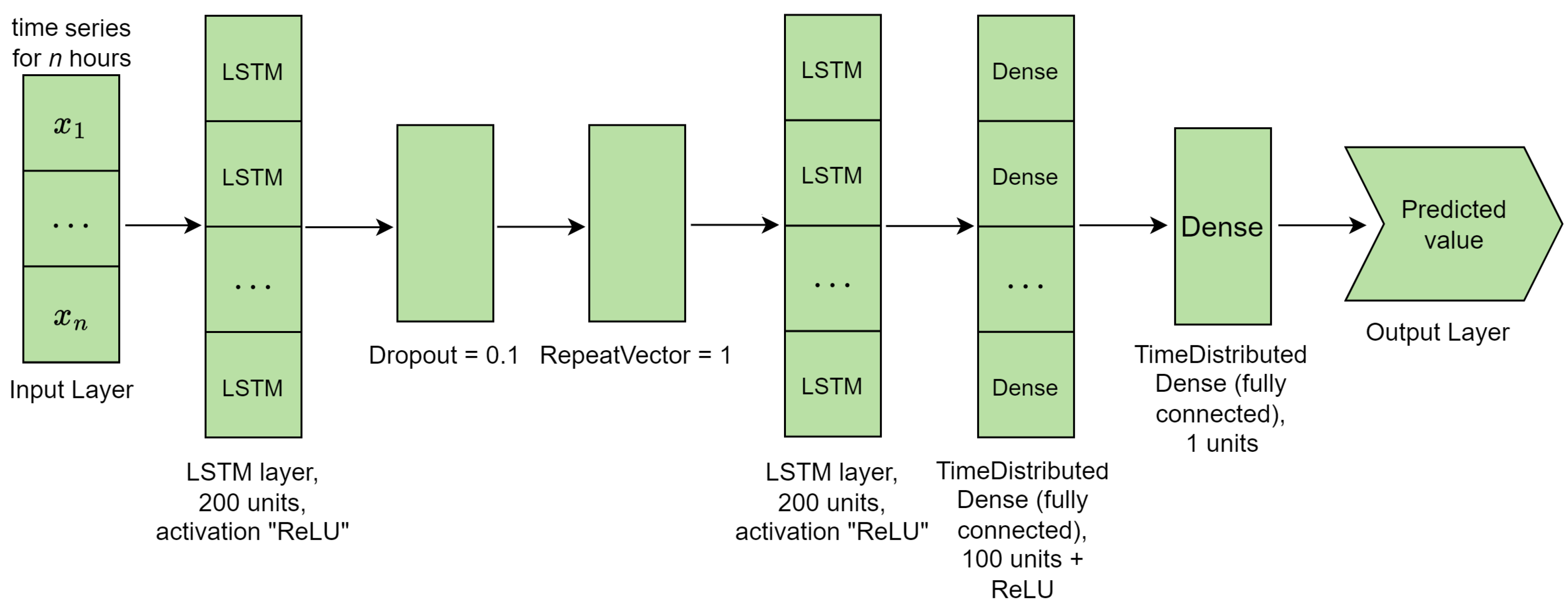
In this phase, several activities are performed sequentially, which take the raw data of air pollution and meteorological factors as input to prepare the input data of the deep learning model both in the training and testing stages, as shown in Figure 1. First, the data extraction activity is executed to create a dataset that maintains the time-series format. This raw dataset of air pollutants and meteorological variables is assigned a window of 60 examples to form instances with the hourly value of the concentration of the contaminants (variables) PM2.5, PM10, and CO, as well as the meteorological variables of relative humidity (RH) and temperature, extracting each of these instances to construct a new time series dataset. A data merging activity is applied following the data transformation. This activity integrates the records of a dataset of wind conditions (recorded in the study period), which contains the values of the variables wind speed, wind direction, date, and time, with the dataset of air pollution and meteorological factors (previously generated). Record merging is performed by comparing the datasets’ date and time values, inserting the values of the wind conditions when the coincidence is true, allowing the records to be aligned, and generating a set of data that will be used as input in the deep learning algorithms.
Next, data normalization through the min–max technique is applied to adjust standardized values in all variables within a range of 0 and 1. This technique allows the data to be standardized. It reduces the impact of differences on the scale and magnitude of data attributes, enabling a comparison of characteristics with different units and ranges of values in the same dataset. For example, the range of values in the temperature variable is between −1 °C and 45 °C, and the values recorded in the relative humidity variable are between 10% and 99%. Finally, the dataset is divided into two sub-datasets, with 80% of the instances for training and 20% for testing data.

3.1.2. Model Design

This phase consists of designing the neural network model based on the characteristics and functionalities of the deep learning architectures to be implemented; in our experiment, we analyze RNN, vanilla LSTM, Stacked LSTM, Bi-LSTM, and encoder–decoder LSTM. Figure 2 shows the Stacked LSTM network built with an LSTM layer followed by a dropout layer. This layer reduces overfitting and improves the model’s generalization. Next, an LSTM layer is appended, which generates a vector that feeds the input of a fully connected multi-layer network, which consists of one dense layer and one output layer. Figure 3 shows the design of the encoder–decoder LSTM neural network, which consists of two parts: an encoder, which is an LSTM network that processes the input sequence, encoding the information into a hidden state vector, and a decoder, which is another LSTM network that uses the hidden state of the encoder output to generate the output sequence. The decoder has two dense output layers that are responsible for producing the output predictions. This dense layer is a standard feedforward layer.
In the next activity of this phase (see Figure 1), we perform hyperparameter optimization for each neural network design by implementing the grid search algorithm. This algorithm calculates and analyzes each combination of hyperparameters using permutation and combination, measuring model performance by three-fold cross-validation on the evaluation set. After performing all possible combinations of hyperparameters, the neural network model that achieves the highest accuracy in the validation process is selected. Then, the configuration of parameters generated by the grid search algorithm is stored.

3.1.3. Train Model

The model selected in the previous phase, considering the best value achieved in the accuracy measure and the loss function, is trained and validated with the dataset generated in the data preprocessing stage (see Figure 1). In the model training phase, the value achieved in the accuracy measure is validated again. If it exceeds a predefined threshold value, it will be used as an LSTM neural network model to predict the concentration level of the contaminant in the next few hours. Otherwise, adjust the hyperparameters of the neural network in the previous stage and train the model again.

3.1.4. Test Model

Finally, after the predictive model has been adequately learned in the training stage, the input data (X) are introduced into a specific matrix structure, as the neural network expects. The input data (X) are the contaminant concentration values at a given time (t). Next, the predictive model predicts the pollutant concentration value (Y) for the next hour ( t + 1 ). The above is performed for all instances of the test dataset, allowing the time series to be constructed with the predicted values for the contaminant concentration. Subsequently, the prediction model’s performance is evaluated using RMSE, the mean absolute error (MAE), the mean square error (MSE), the mean absolute percentage error (MAPE), mean bias error (MBE), and the coefficient of determination (R2).

3.2. Dataset

The air pollution dataset used in our experiment comprises records from 1 January 2020 to 30 June 2020, collected in Victoria City, located in the northeastern region of Mexico. Victoria is the political capital of the state of Tamaulipas, with a population of 350,000 inhabitants in 2020 and an area of 200 km2. Figure 4 shows the location of the air quality monitoring stations at the neighborhood level to monitor residential, downtown, industrial, and commercial areas. The prevailing winds were from the southeast for most of the year, and the average annual temperature (2020) was 26 °C, with minimum values of 0 °C and maximum values of 42 °C. The city is located next to an extensive mountainous area. The data correspond to the monitoring station located southeast of the town. This station records the highest levels of air pollution, characterized by a large flow of vehicles. It is located near an industrial park, government buildings, and a sanitary landfill. The dataset contains the attributes of the PM2.5, PM10, CO, relative humidity (RH), temperature (T), heat index (HI), wind direction (WD), and wind speed (WS), as shown in [42,43]. Figure 5 shows the time series of six of the eight variables used in the study, considering all the records in the dataset. The hourly average was calculated from these raw data, with 4368 records. Subsequently, the records from 01/01/2020 01:00:00 to 05/25/2020 13:00:00 were filtered, representing 80% (3493 records) of the dataset to construct the sub-dataset training used in the five deep learning architectures. The remaining records from05/25/2020 14:00:00 to 06/30/2020 23:59:59 make up the sub-dataset for the testing stage, totaling 875 records.

3.3. Measurement

To assess the prediction performance of the proposed neural network models, we adopted six evaluation indicators, RMSE, MAE, MSE, MAPE, MBE, and R2, given by Equations (1)–(6):
R M S E = 1 n i = 1 n ( y i y ^ i ) 2
M A E = 1 n i = 1 n y i y ^ i
M S E = 1 n i = 1 n ( y i y ^ i ) 2
M A P E = 1 n i = 1 n y i y ^ i y i × 100
M B E = 1 n i = 1 n ( y i y ^ i )
R 2 = 1 i = 1 n ( y i y ^ i ) 2 i = 1 n ( y i y ¯ i ) 2
where y i denotes the actual value, y ^ i indicates the predicted value, y ¯ i is the mean of observed values, and n represents the sample size.

4. Results

The evaluation of the prediction results of the models seeks to know the accuracy and performance, considering that the lower the values of RMSE and MAE, the higher the accuracy of the model, and the closer the value of R2 is to 1, the higher the model’s performance. Table 1 shows the performance achieved by the deep learning models in predicting the concentration level of the pollutant PM2.5, observing that the models reach values in the error metrics very close to zero. It is highlighted that the Stacked LSTM model obtains a 3.4538 μg/m3 in the RMSE metric, which is the lowest error measured in the prediction of the five deep learning architectures implemented. This deep learning model in the MAE metric obtains a value of 2.2478 μg/m3, which means that the average difference between the predicted and actual PM2.5 concentration level will be 2.2455 μg/m3. The Vanilla LSTM model obtained results very close to those of the Stacked LSTM model, with values of 3.4647 μg/m3 and 2.2554 μg/m3 for the RMSE and MAE metrics, respectively (see Table 1).
Figure 6 and Figure 7 show the visualization of the prediction results in the Stacked LSTM and Vanilla LSTM architectures, respectively. The blue line represents the time series of the original or real data, and the red line represents the time series with the values predicted by the model. The X-axis shows the time (hours), and the Y-axis represents the value of the concentration of the PM2.5 pollutant measured in μg/m3. Additionally, the permissible limit values of PM2.5 concentrations (for 24 h) of 25 μg/m3 and 35 μg/m3 have been marked (in both figures) as a reference, with a green dashed line according to the official Mexican Environmental Health Standard [44] and with an orange dashed line according to the National Ambient Air Quality Standards (NAAQS) of the United States Environmental Protection Agency (USEPA) [45]. Figure 6 shows how the data predicted by the Stacked LSTM model fit the data observed in most of the hours in the testing dataset used in the experiment. In cases where the PM2.5 concentration exceeds 43 μg/m3, the predicted PM2.5 concentration is underestimated, as identified in the peaks at 05/27/2020 05:00:00 (X-axis) and between 06/02/2020 07:00:00 and 06/03/2020 23:00:00 (X-axis). However, the model overestimates a more significant number of cases, as seen in most predicted concentration values between 30 and 40 μg/m3 (Y-axis) during 06/17/2020 and 06/27/2020 (X-axis). This overestimation and underestimation of the pollutant concentration are very slight, verified by the value reached close to zero (0.0232) in the MBE metric (see Table 1).
On the other hand, Figure 7 shows how the time series predicted by the Vanilla LSTM model aligns with the real air pollutant data, and its behavior is very similar to the prediction made by the Stacked LSTM model. However, it presents more cases of overestimating and underestimating PM2.5 concentration, which is validated by the obtained value of −0.1806 in the MBE metric, indicating an underestimation of the predicted values. For example, at very low PM2.5 concentration levels (between 2 μg/m3 and 4 μg/m3), the Vanilla LSTM model slightly overestimates the predicted value, observed between 06/07/2020 07:00:00 and 06/10/2020 05:00:00 (X-axis). Likewise, in Figure 7, several cases of underestimation are observed between 05/25/2020 and 06/06/2020 when the model predicts concentration values between 20 and 40 μg/m3. It is essential to highlight that the overestimated or underestimated data are scant (in both models) compared to the real data. The slight difference is verified with the evaluation using the error metrics (see Table 1). For example, in measuring the quality of fit of the Stacked LSTM and Vanilla LSTM models, RMSEs of 3.4538 μg/m3 and 3.4647 μg/m3 were obtained, which were very close to a perfect fit. In addition, it was identified that the permissible limit value for a 24-h PM2.5 concentration was exceeded on day six, according to the Mexican Official Standard, and on day two, according to the EPA standard, recording a maximum daily average of 42.31 μg/m3.
Table 2 shows the results of evaluating the deep learning models used in the dataset to predict the PM10 pollutant. When we compared the performance of the models considering the RMSE, MAE, and R2 metrics, it was identified that the prediction performance is in the order of encoder–decoder LSTM, Vanilla LSTM, Bi-LSTM, Stacked LSTM, and RNN. Therefore, the encoder–decoder LSTM model demonstrates superior results in the evaluation, obtaining an RMSE of 3.2606, which indicates that the predictions of this model exhibit a deviation of around 3.26 μg/m3 from the actual values of the air pollutant. In this sense, the MAE score of 2.10 indicates that the prediction results of the encoder–decoder LSTM model exhibit an average variation of 2.10 μg/m3 concerning the actual values of the PM10 concentration. Moreover, Table 2 shows that most of the prediction models evaluated obtain an R2 of around 0.90. For example, the R2 value of 0.8979 means that the encoder–decoder LSTM model is highly precise in capturing the patterns discovered in the data and correctly represents how the proportion of the variance in the dependent variable (PM10) is predictable from the predictor variables [46].
Figure 8 shows the prediction of the PM10 concentration values generated by the encoder–decoder LSTM model, displaying a very close fit of the predicted data with the original data; that is, the predicted PM10 concentration in most cases is similar to the actual data, reaching a very acceptable value of −0.0227 in the MBE measurement. The prediction model sometimes overestimates the predicted concentration value for peaks above 46 μg/m3, as seen for values recorded between 06/03/2020 19:00:00 and 06/04/2020 22:00:00. On the contrary, at low concentration values (e.g., between 1 and 10 μg/m3), the encoder–decoder LSTM model underestimates the pollutant concentration values as shown by the predicted values between 06/06/2020 01:00:00 and 06/14/2020 09:00:00. Furthermore, in Figure 8 and Figure 9, the concentration of 50 μg/m3 was defined as the maximum permissible limit for PM10 (green dashed line) for 24 h, according to the official Mexican Environmental Health Standard [44]. This concentration limit was exceeded by up to 30% on 14 occasions (days) during the monitoring period considered for the training stage and on one occasion during the testing stage of the prediction models.
Figure 9 depicts the regression values of the PM10 concentration using the Vanilla LSTM model compared to the actual measurements using the validation dataset. This figure shows that the model can identify PM10 peaks during the evaluated period. Similar to the encoder–decoder LSTM model, it closely followed the behavior of the actual data during the test period, indicating a good performance of the model. It is important to emphasize that the model’s overestimation and underestimation are greater than the encoder–decoder LSTM model, reflected in the MBE metric value of −0.1460, denoting an underestimation in the model predictions. The above can be seen in the overestimation from 06/03/2020 19:00:00 to 06/04/2020 22:00:00, and in the underestimation observed between 06/06/2020 01:00:00 and 06/14/2020 09:00:00, the same ranges of instances analyzed for the previous model.
Table 3 compares CO prediction accuracy using the five deep learning models and time series as input variables. When all the time series considered for the model testing stage are used (875 records), an R2 of 0.9799 and an RMSE of 0.1117 ppm are obtained using the encoder–decoder LSTM model, demonstrating its learning capacity in different sets of air pollution data. This prediction model obtains the lowest MAE of the study with a value of 0.0556 ppm, very close to 0. The results shown in Table 3 highlight the performance achieved by the RNN model, with values of 0.1222 ppm, 0.0708 ppm, and 0.9754 for RMSE, MAE, and R2, respectively. The models based on stacked LSTM and Bi-LSTM obtain values that are very close to each other in all evaluation metrics consistent with the two previous experiments, which means both models learn similarly from 3493 instances used in the training stage, achieving good results in predicting the CO concentration level per hour.
The decrease in the CO concentration reported in the testing dataset was recorded during the second and third months of the COVID-19 pandemic, a period in which mobility restrictions were more rigid (industrial, commercial, transportation, services, and education activities were suspended, and only essential activities remained active). Also, rainfall occurred for several weeks during this period, causing an extreme decrease in CO pollution levels. Figure 10 shows the time series of hourly CO concentration measurements and predictions from the encoder–decoder LSTM model. This model reproduces the peaks and general behavior of CO concentration levels; at high concentration values, an underprediction is observed between 05/28/2020 01:00:00 and 05/30/2020 19:00:00 (X-axis). Furthermore, it is identified that the model adequately learned the behavior of the pollutant concentration and its relationship with the predictor variables, demonstrating that the model has the capacity to predict the behavior of the pollutant CO correctly and can even predict the considerable decrease that occurs at hour 05/31/2020 23:00:00 (X-axis), with a drastic reduction from 0.55 ppm to 0.08 ppm, which continues the rest of the instances of the test dataset in a range of 0.03 ppm and 0.05 ppm. At this stage, the model continues with a prediction very close to the actual data, even at the peak of 0.24 ppm at 06/04/2020 03:00:00 (X-axis). Moreover, in the last hours of the prediction diagram between 06/25/2020 05:00:00 and 06/30/2020 24:00:00 h (X-axis), a slight overprediction is observed in the measurement of the CO concentration by the encoder–decoder LSTM model, which is recorded by the MBE metric with an average value of 0.0186 (see Table 3). This demonstrates a very low overestimation of the model since it is very close to zero.
Figure 11 compares the measured CO concentration (actual) and the concentration predicted by the RNN model. This model overpredicts and underpredicts the value of the CO concentration when peaks and decreases in high values occur, as observed in the behavior from 05/25/2020 14:00:00 to 05/31/2020 24:00:00 h (X-axis). At low concentration values, it correctly follows the behavior of the real data in the time series but with a slight overestimation, which aligns with the value reached in the MBE measurement of 0.0239. Notably, this model demonstrated its ability to identify the drastic decrease in the CO concentration contained in the test dataset, which is a behavior with a high level of complexity. In addition, the mean recorded for the CO concentration for 1 h or 8 h in our experiment is very far from the permissible limit value of 26 ppm (1 h) and 9 ppm (8 h) [44].

5. Discussion

Deep learning algorithms have been implemented to predict future events in complex (e.g., numerous pollution sources) and non-linear problem contexts. In most cases, with their superior forecasting capabilities, deep learning-based approaches outperform traditional methods in predicting the future concentration of air pollutants. In predicting the air quality index (AQI), hybrid CNN-Bi-LSTM algorithms have been used [47], demonstrating high accuracy. LSTM has achieved excellent performance in hourly AQI predictions [48], and hybrid CNN-LSTM algorithms have been optimized with the capacity to reduce the high dimensionality of characteristics in industrial areas [49]. Next, the main approaches with a similar objective to our proposal are discussed.
In [50], the authors evaluated the ability of an RNN-based model to predict the hourly concentration of criterion air pollutants and two air quality indices. For the pollutant PM2.5, they obtained an RMSE value of 82.6 μg/m3, using 5% of the instances in the dataset for the model testing stage. Similarly, [51] proposed a hybrid model based on a spatiotemporal convolutional LSTM neural network that can predict the concentration of PM2.5 from 1 to 24 h for different monitoring stations. The dataset contains concentration values from 1233 monitoring stations for approximately 24 months, considering the variables of relative humidity, temperature, and wind speed. The model performance reaches an RMSE of 12.08 μg/m3 in the prediction of the 1st hour, and in the prediction of the 13th hour to the 24th hour, the RMSE rises to 23.18 μg/m3. The authors [22] proposed a prediction model that combines three LSTM models to realize early (1 to 8 h) prediction of air pollutant PM2.5. The model is trained with 5-year instances using data from Taiwan’s air quality monitoring stations, data from stations near industrial zones, and external data referring to monitoring stations located within a radius of 50 km. In the average prediction for the next hour of PM2.5, an RMSE of 3.94 μg/m3 is obtained. For the next eighth hour, an RMSE of 7.6 μg/m3 is acquired; according to the authors, the prediction of the concentration of PM2.5 in our experiment presents an underestimation.
For their part, the authors in [25] proposed two prediction models based on LSTM optimized with particle swarm optimization (PSO) and sparrow search algorithm (SSA) meta-heuristics. The dataset contains values from nine air quality monitoring stations, including six criterion air pollutants and five meteorological factors for 12 months. The LTSM models were trained with 70% of the instances in the dataset, and the PM2.5 target prediction was for two monitoring stations in Kuala Lumpur, Malaysia. The LSTM models that obtain the highest performance include the predictor variables of PM10, NO2, O3, CO, temperature, and relative humidity. The PSO-LSTM model reached 8.1646 μg/m3 and 9.2711 μg/m3 in the RMSE metric for monitoring stations 1 and 2, respectively. On the other hand, the SSA-LSTM model obtained RMSE values of 8.0933 μg/m3 and 9.2533 μg/m3 for monitoring stations 1 and 2, respectively. Finally, in [52], they proposed an optimized hybrid prediction model approach based on CNN and LSTM neural networks for PM2.5. Additionally, they validated the impact on model performance by including the concentration of air pollutants PM10, CO, SO2, NO2, and O3 as predictor variables. The authors confirm that these variables contribute significantly to predicting PM2.5 concentration in all experiments. The prediction performance is validated with an RMSE between 10.699 μg/m3 and 12.68 μg/m3 in the different study cases. Other approaches have been presented where the authors propose the long-term prediction of the concentration of air pollutants by considering the spatial level of the data; in [33], the authors propose a hybrid model based on a graph neural network (GNN) and an LSTM network to manage the spatiotemporal correlations and improve the identification of the influence of the transport of pollutants in space. The GNN-LSTM model performs well in predicting the long-term concentration level of PM2.5 (72 h). In [37], the authors expose the performance of the GNN model for predicting the concentration of PM2.5 through a spatiotemporal approach, obtaining a high performance according to the evaluation metrics. Similarly, the authors of [53] present a GNN model for short-term PM2.5 concentrations that obtain good results in predicting environments with high air pollution concentration levels.
On the other hand, [54] proposed several topologies for LSTM to predict the concentration of PM10, which is highlighted by the use of a historical dataset with 12-year records for training the LSTM neural network and a set of data with 1-year instances for the testing stage of three air quality monitoring stations in Madrid, Spain. The prediction model achieved its best performance with an RMSE of 5.350 μg/m3, and on average, of the three monitoring stations, it obtained an RMSE of 5.721 μg/m3 in the prediction of the air pollutant PM10. In [55], a comparison of the performance of prediction models based on LSTM, RNN, and multiple linear regression is presented. This comparison is conducted to predict the concentration of PM10 in a port area in South Korea. The study utilizes a dataset with 7034 instances (20% is used for model testing) that contain hourly average values of PM2.5, PM10, NO2, CO, SO2, O3, temperature, relative humidity, wind, speed, rainfall, and three variables with port operation data (number of trucks, anchored vessels, and capacity/gross weight of anchored vessels). The authors report that the best performance is obtained by the LSTM model (RMSE = 20.943) when using only data on air pollutants and meteorological factors. When port operation data are considered in the input vectors to train the model, the RNN (RMSE = 20.782) slightly outperforms the LSTM model (RMSE = 20.814) in predicting PM10 concentration. Similarly, in [56], they propose a comparison between machine learning algorithms versus deep learning to predict the concentration of PM10, reporting that an artificial neural network optimized with the Levenberg–Marquardt algorithm to solve non-linear least squares problems obtains better performance in predicting PM10 concentration, surpassing an LSTM model. In [57], they proposed an approach combining the K-means clustering algorithm and an LSTM neural network to form groups of monitoring stations based on the similarity in the concentration levels of air pollutants, which allowed them to create prediction models per identified cluster. The performance of the prediction model for the PM10 concentration level is acceptable when data derived from clusters are used. However, in most cases, the lower values in the error metrics are obtained in the individual prediction models.
Regarding the prediction of CO, the authors of [58] reported the evaluation of statistical and deep learning models to predict air pollution by CO; with a model based on seasonal-LSTM, they obtained an average RMSE of 0.0118 ppm and an R2 of 0.94 using data collected at 10 air quality monitoring stations. Similarly, Navares and Aznarte [54] obtained an average RMSE of the seven monitoring stations of 0.083 ppm for predicting future CO concentrations, with the best RMSE of 0.059 ppm and the worst RMSE of 0.111 ppm from different monitoring stations considered in your study.The authors in [59] evaluated the performance of two prediction models based on LSTM and BiLSTM to predict the daily concentration of CO. Therefore, they developed six scenarios with real data on the concentration of CO and PM10 based on the high correlation identified between these pollutants, including in the dataset the instances of 5 years with the daily concentration value. The LSTM model obtained an RMSE of 195.6, and the performance of the BiLSTM model is very close, with a value of 203 in the same metric. In another experiment, they evaluated the performance of an LSTM model with different hyperparameters for predicting CO concentration in a port area using 6-hour intervals in their dataset [60].
In our approach, the prediction models based on Vanilla LSTM, Stacked LSTM, and encoder–decoder LSTM obtain close performance, with an R2 of around 90 in the PM2.5 prediction. Similarly, in predicting the future hourly concentration of PM10 and CO, the encoder–decoder LSTM neural network obtained the best performance, slightly outperforming the vanilla LSTM and RNN networks, with a difference of 0.0017 and 0.0045 in R2, respectively. Although a direct comparison cannot be made with previous research because the same dataset is not used, they can be taken as a reference because, in most cases, the same predictor variables are used (air pollutants and meteorological factors) to predict the future value of the target air pollutant concentration. The performance of the prediction models demonstrates stability throughout the prediction hours, which we relate to the data preprocessing stage carried out, as well as the optimization of the hyperparameters of the different neural networks and the defined architectural design in each LSTM model.

6. Conclusions

This work presents the results of a comprehensive evaluation of different air pollution prediction models derived from the LSTM neural network. It has been found that models based on deep learning architectures can accurately predict hourly air pollution with fewer predictor variables, ensuring their reliability. This performance may be conditioned by the behavior identified in the data contained in the variables, the dependence between the data, the volume of data available for training the model, and the quality of the data. The normalization of the data on the concentration of air pollutants and meteorological factors involved transforming the data to a standard scale, which improved the model’s performance. The optimization of hyperparameters of the LSTM models was performed using a grid search method, which helped to find the best combination of parameters for each model. These steps, along with the architectural design of the neural network, significantly benefited the accuracy of the prediction models, as shown in the error metrics and coefficient of determination results, which are very close between the different prediction models. The proposed prediction models have been rigorously tested and have demonstrated a very close forecast accuracy in the three air pollutants analyzed. This high level of accuracy, combined with the optimization of hyperparameters in the different models, strengthens the deep neural networks’ discrimination capacity, thereby instilling confidence in the models’ reliability and the research’s trustworthiness to contribute to the sustainable development of cities through comprehensive air pollution management.

Author Contributions

Conceptualization, E.T.-L. and U.M.R.-A.; methodology, E.T.-L. and U.M.R.-A.; software, U.M.R.-A.; validation, E.T.-L., U.M.R.-A., B.A.M.-H. and J.D.H.-R.; formal analysis, E.T.-L. and U.M.R.-A.; investigation, E.T.-L., U.M.R.-A., B.A.M.-H. and J.D.H.-R.; resources, E.T.-L.; data curation, E.T.-L. and U.M.R.-A.; writing—original draft preparation, E.T.-L., U.M.R.-A. and B.A.M.-H.; writing—review and editing, E.T.-L., U.M.R.-A., B.A.M.-H. and J.D.H.-R.; visualization, U.M.R.-A.; supervision, E.T.-L.; project administration, E.T.-L.; funding acquisition, E.T.-L. All authors have read and agreed to the published version of the manuscript.

Funding

This research was partially supported by the Consejo Nacional de Ciencia y Tecnología (CONACYT) of México under grant number 748457.

Institutional Review Board Statement

Not applicable.

Informed Consent Statement

Not applicable.

Data Availability Statement

Dataset available on request from the authors.

Acknowledgments

The authors are grateful to the Autonomous University of Tamaulipas, Mexico, for supporting this work.

Conflicts of Interest

The authors declare no conflicts of interest.

Abbreviations

The following abbreviations are used in this manuscript:
DLDeep learning
LSTMLong short-term memory
Bi-LSTMBidirectional long short-term memory
RNNRecurrent neural networks
RMSERoot mean square error
MAEMean absolute error
MSEMean square error
MAPEMean absolute percentage error
R2Determination coefficient
PM2.5Particulate matter < 10 μm
PM10Particulate matter < 2.5 μm
COCarbon monoxide

References

  1. Delavar, M.A.; Jahani, M.A.; Sepidarkish, M.; Alidoost, S.; Mehdinezhad, H.; Farhadi, Z. Relationship between fine particulate matter (PM2.5) concentration and risk of hospitalization due to chronic obstructive pulmonary disease: A systematic review and meta-analysis. BMC Public Health 2023, 23, 2229. [Google Scholar] [CrossRef] [PubMed]
  2. Anenberg, S.C.; Mohegh, A.; Goldberg, D.L.; Kerr, G.H.; Brauer, M.; Burkart, K.; Hystad, P.; Larkin, A.; Wozniak, S.; Lamsal, L. Long-term trends in urban NO2 concentrations and associated pediatric asthma incidence: Estimates from global datasets. Lancet Planet. Health 2022, 6, e49–e58. [Google Scholar] [CrossRef] [PubMed]
  3. Andreão, W.L.; Toledo de Almeida Albuquerque, T. Avoidable mortality by implementing more restrictive fine particles standards in Brazil: An estimation using satellite surface data. Environ. Res. 2021, 192, 110288. [Google Scholar] [CrossRef] [PubMed]
  4. Domingo, J.L.; Rovira, J. Effects of air pollutants on the transmission and severity of respiratory viral infections. Environ. Res. 2020, 187, 109650. [Google Scholar] [CrossRef] [PubMed]
  5. Gutman, L.; Pauly, V.; Orleans, V.; Piga, D.; Channac, Y.; Armengaud, A.; Boyer, L.; Papazian, L. Long-term exposure to ambient air pollution is associated with an increased incidence and mortality of acute respiratory distress syndrome in a large French region. Environ. Res. 2022, 212, 113383. [Google Scholar] [CrossRef] [PubMed]
  6. Liu, C.; Yin, P.; Chen, R.; Meng, X.; Wang, L.; Niu, Y.; Lin, Z.; Liu, Y.; Liu, J.; Qi, J.; et al. Ambient carbon monoxide and cardiovascular mortality: A nationwide time-series analysis in 272 cities in China. Lancet Planet. Health 2018, 2, e12–e18. [Google Scholar] [CrossRef] [PubMed]
  7. Liu, Y.; You, J.; Dong, J.; Wang, J.; Bao, H. Ambient carbon monoxide and relative risk of daily hospital outpatient visits for respiratory diseases in Lanzhou, China. Int. J. Biometeorol. 2023, 67, 1913–1925. [Google Scholar] [CrossRef]
  8. Taheri, M.; Nouri, F.; Ziaddini, M.; Rabiei, K.; Pourmoghaddas, A.; Islam, S.M.S.; Sarrafzadegan, N. Ambient carbon monoxide and cardiovascular-related hospital admissions: A time-series analysis. Front. Physiol. 2023, 14, 1–9. [Google Scholar] [CrossRef] [PubMed]
  9. Goldsborough, E.; Gopal, M.; McEvoy, J.W.; Blumenthal, R.S.; Jacobsen, A.P. Pollution and cardiovascular health: A contemporary review of morbidity and implications for planetary health. Am. Heart J. Plus Cardiol. Res. Pract. 2023, 25, 100231. [Google Scholar] [CrossRef] [PubMed]
  10. Chillrud, S.N.; Ae-Ngibise, K.A.; Gould, C.F.; Owusu-Agyei, S.; Mujtaba, M.; Manu, G.; Burkart, K.; Kinney, P.L.; Quinn, A.; Jack, D.W.; et al. The effect of clean cooking interventions on mother and child personal exposure to air pollution: Results from the Ghana Randomized Air Pollution and Health Study (GRAPHS). J. Expo. Sci. Environ. Epidemiol. 2021, 31, 683–698. [Google Scholar] [CrossRef] [PubMed]
  11. Kaali, S.; Jack, D.W.; Mujtaba, M.N.; Chillrud, S.N.; Ae-Ngibise, K.A.; Kinney, P.L.; Boamah Kaali, E.; Gennings, C.; Colicino, E.; Osei, M.; et al. Identifying sensitive windows of prenatal household air pollution on birth weight and infant pneumonia risk to inform future interventions. Environ. Int. 2023, 178, 108062. [Google Scholar] [CrossRef] [PubMed]
  12. Alexander, D.A.; Northcross, A.; Karrison, T.; Morhasson-Bello, O.; Wilson, N.; Atalabi, O.M.; Dutta, A.; Adu, D.; Ibigbami, T.; Olamijulo, J.; et al. Pregnancy outcomes and ethanol cook stove intervention: A randomized-controlled trial in Ibadan, Nigeria. Environ. Int. 2018, 111, 152–163. [Google Scholar] [CrossRef] [PubMed]
  13. Wylie, B.J.; Kishashu, Y.; Matechi, E.; Zhou, Z.; Coull, B.; Abioye, A.I.; Dionisio, K.L.; Mugusi, F.; Premji, Z.; Fawzi, W.; et al. Maternal exposure to carbon monoxide and fine particulate matter during pregnancy in an urban Tanzanian cohort. Indoor Air 2017, 27, 136–146. [Google Scholar] [CrossRef] [PubMed]
  14. Méndez, M.; Merayo, M.G.; Núñez, M. Machine learning algorithms to forecast air quality: A survey. Artif. Intell. Rev. 2023, 56, 10031–10066. [Google Scholar] [CrossRef] [PubMed]
  15. Bekkar, A.; Hssina, B.; Douzi, S.; Douzi, K. Air-pollution prediction in smart city, deep learning approach. J. Big Data 2021, 8, 161. [Google Scholar] [CrossRef] [PubMed]
  16. Kalajdjieski, J.; Zdravevski, E.; Corizzo, R.; Lameski, P.; Kalajdziski, S.; Pires, I.M.; Garcia, N.M.; Trajkovik, V. Air Pollution Prediction with Multi-Modal Data and Deep Neural Networks. Remote Sens. 2020, 12, 4142. [Google Scholar] [CrossRef]
  17. Xia, W.; Zhu, W.; Liao, B.; Chen, M.; Cai, L.; Huang, L. Novel architecture for long short-term memory used in question classification. Neurocomputing 2018, 299, 20–31. [Google Scholar] [CrossRef]
  18. Kim, J.; Lee, H.; Lee, M.; Han, H.; Kim, D.; Kim, H.S. Development of a Deep Learning-Based Prediction Model for Water Consumption at the Household Level. Water 2022, 14, 1512. [Google Scholar] [CrossRef]
  19. Karasu, S.; Altan, A. Crude oil time series prediction model based on LSTM network with chaotic Henry gas solubility optimization. Energy 2022, 242, 122964. [Google Scholar] [CrossRef]
  20. Ma, C.; Dai, G.; Zhou, J. Short-Term Traffic Flow Prediction for Urban Road Sections Based on Time Series Analysis and LSTM_BILSTM Method. IEEE Trans. Intell. Transp. Syst. 2022, 23, 5615–5624. [Google Scholar] [CrossRef]
  21. Men, L.; Ilk, N.; Tang, X.; Liu, Y. Multi-disease prediction using LSTM recurrent neural networks. Expert Syst. Appl. 2021, 177, 114905. [Google Scholar] [CrossRef]
  22. Chang, Y.S.; Chiao, H.T.; Abimannan, S.; Huang, Y.P.; Tsai, Y.T.; Lin, K.M. An LSTM-based aggregated model for air pollution forecasting. Atmos. Pollut. Res. 2020, 11, 1451–1463. [Google Scholar] [CrossRef]
  23. Kristiani, E.; Lin, H.; Lin, J.R.; Chuang, Y.H.; Huang, C.Y.; Yang, C.T. Short-Term Prediction of PM2.5 Using LSTM Deep Learning Methods. Sustainability 2022, 14, 2068. [Google Scholar] [CrossRef]
  24. Das, B.; Dursun, Ö.O.; Toraman, S. Prediction of air pollutants for air quality using deep learning methods in a metropolitan city. Urban Clim. 2022, 46, 101291. [Google Scholar] [CrossRef]
  25. Zaini, N.; Ahmed, A.N.; Ean, L.W.; Chow, M.F.; Malek, M.A. Forecasting of fine particulate matter based on LSTM and optimization algorithm. J. Clean. Prod. 2023, 427, 139233. [Google Scholar] [CrossRef]
  26. Kim, Y.-B.; Park, S.B.; Lee, S.; Park, Y.K. Comparison of PM2.5 prediction performance of the three deep learning models: A case study of Seoul, Daejeon, and Busan. J. Ind. Eng. Chem. 2023, 120, 159–169. [Google Scholar] [CrossRef]
  27. Eren, B.; Aksangür, İ; Erden, C. Predicting next hour fine particulate matter (PM2.5) in the Istanbul Metropolitan City using deep learning algorithms with time windowing strategy. Urban Clim. 2023, 48, 101418. [Google Scholar] [CrossRef]
  28. Zhang, L.; Liu, P.; Zhao, L.; Wang, G.; Zhang, W.; Liu, J. Air quality predictions with a semi-supervised bidirectional LSTM neural network. Atmos. Pollut. Res. 2021, 12, 328–339. [Google Scholar] [CrossRef]
  29. Wang, S.; Ren, Y.; Xia, B.; Liu, K.; Li, H. Prediction of atmospheric pollutants in urban environment based on coupled deep learning model and sensitivity analysis. Chemosphere 2023, 331, 138830. [Google Scholar] [CrossRef] [PubMed]
  30. Gilik, A.; Ogrenci, A.S.; Ozmen, A. Air quality prediction using CNN+LSTM-based hybrid deep learning architecture. Environ. Sci. Pollut. Res. 2022, 29, 11920–11938. [Google Scholar] [CrossRef] [PubMed]
  31. Yang, G.; Lee, H.; Lee, G. A Hybrid Deep Learning Model to Forecast Particulate Matter Concentration Levels in Seoul, South Korea. Atmosphere 2020, 11, 348. [Google Scholar] [CrossRef]
  32. Oliveira Santos, V.; Costa Rocha, P.A.; Scott, J.; Van Griensven Thé, J.; Gharabaghi, B. Spatiotemporal Air Pollution Forecasting in Houston-TX: A Case Study for Ozone Using Deep Graph Neural Networks. Atmosphere 2023, 14, 308. [Google Scholar] [CrossRef]
  33. Teng, M.; Li, S.; Xing, J.; Fan, C.; Yang, J.; Wang, S.; Song, G.; Ding, Y.; Dong, J.; Wang, S. 72-hour real-time forecasting of ambient PM2.5 by hybrid graph deep neural network with aggregated neighborhood spatiotemporal information. Environ. Int. 2023, 176, 107971. [Google Scholar] [CrossRef] [PubMed]
  34. Dun, A.; Yang, Y.; Lei, F. Dynamic graph convolution neural network based on spatial-temporal correlation for air quality prediction. Ecol. Inform. 2022, 70, 101736. [Google Scholar] [CrossRef]
  35. Zhang, C.; Wang, S.; Wu, Y.; Zhu, X.; Shen, W. A long-term prediction method for PM2.5 concentration based on spatiotemporal graph attention recurrent neural network and grey wolf optimization algorithm. J. Environ. Chem. Eng. 2024, 12, 111716. [Google Scholar] [CrossRef]
  36. Mao, W.; Jiao, L.; Wang, W.; Wang, J.; Tong, X.; Zhao, S. A hybrid integrated deep learning model for predicting various air pollutants. GISci. Remote Sens. 2021, 58, 1395–1412. [Google Scholar] [CrossRef]
  37. Jin, X.B.; Wang, Z.Y.; Kong, J.L.; Bai, Y.T.; Su, T.L.; Ma, H.J.; Chakrabarti, P. Deep Spatio-Temporal Graph Network with Self-Optimization for Air Quality Prediction. Entropy 2023, 25, 247. [Google Scholar] [CrossRef] [PubMed]
  38. Huang, Y.; Ying, J.J.C.; Tseng, V.S. Spatio-attention embedded recurrent neural network for air quality prediction. Knowl.-Based Syst. 2021, 233, 107416. [Google Scholar] [CrossRef]
  39. Yan, X.; Zang, Z.; Jiang, Y.; Shi, W.; Guo, Y.; Li, D.; Zhao, C.; Husi, L. A Spatial-Temporal Interpretable Deep Learning Model for improving interpretability and predictive accuracy of satellite-based PM2.5. Environ. Pollut. 2021, 273, 116459. [Google Scholar] [CrossRef]
  40. Fu, Q.; Guo, H.; Gu, X.; Li, J.; Zhang, W.; Mi, X.; Zhao, Q.; Chen, D. High-Resolution PM2.5 Concentrations Estimation Based on Stacked Ensemble Learning Model Using Multi-Source Satellite TOA Data. Remote Sens. 2023, 15, 5489. [Google Scholar] [CrossRef]
  41. Tian, L.; Chen, L.; Zhang, P.; Hu, B.; Gao, Y.; Si, Y. The Ground-Level Particulate Matter Concentration Estimation Based on the New Generation of FengYun Geostationary Meteorological Satellite. Remote Sens. 2023, 15, 1459. [Google Scholar] [CrossRef]
  42. Tello-Leal, E.; Macías-Hernández, B.A. Association of environmental and meteorological factors on the spread of COVID-19 in Victoria, Mexico, and air quality during the lockdown. Environ. Res. 2021, 196, 110442. [Google Scholar] [CrossRef] [PubMed]
  43. Ramirez-Alcocer, U.M.; Tello-Leal, E.; Macías-Hernández, B.A.; Hernandez-Resendiz, J.D. Data-Driven Prediction of COVID-19 Daily New Cases through a Hybrid Approach of Machine Learning Unsupervised and Deep Learning. Atmosphere 2022, 13, 1205. [Google Scholar] [CrossRef]
  44. Gobierno de México—SEMARNAT. Normas Oficiales Mexicanas (NOM) de Calidad del Aire Ambiente. 2024. Available online: https://www.gob.mx/cof\protect\discretionary{\char\hyphenchar\font}{}{}epris/acciones-y-programas/4-normas-oficiales-mexicanas-nom-de-calidad-del-aire-ambiente (accessed on 31 July 2024).
  45. United States Environmental Protection Agency (EPA). Criteria Air Pollutants. 2024. Available online: https://www.epa.gov/criteria-air-pollutants/naaqs-table (accessed on 31 July 2024).
  46. Chicco, D.; Warrens, M.J.; Jurman, G. The coefficient of determination R-squared is more informative than SMAPE, MAE, MAPE, MSE and RMSE in regression analysis evaluation. PeerJ Comput. Sci. 2021, 7, e623. [Google Scholar] [CrossRef] [PubMed]
  47. Rabie, R.; Asghari, M.; Nosrati, H.; Emami Niri, M.; Karimi, S. Spatially resolved air quality index prediction in megacities with a CNN-Bi-LSTM hybrid framework. Sustain. Cities Soc. 2024, 109, 105537. [Google Scholar] [CrossRef]
  48. Mishra, A.; Gupta, Y. Comparative analysis of Air Quality Index prediction using deep learning algorithms. Spat. Inf. Res. 2024, 32, 63–72. [Google Scholar] [CrossRef]
  49. Zhanga, R.; Tang, J.; Xia, H.; Pan, X.; Yu, W.; Qiao, J. CO emission predictions in municipal solid waste incineration based on reduced depth features and long short-term memory optimization. Neural Comput. Appl. 2024, 36, 5473–5498. [Google Scholar] [CrossRef]
  50. Maleki, H.; Sorooshian, A.; Goudarzi, G.; Baboli, Z.; Birgani, Y.T.; Rahmati, M. Air pollution prediction by using an artificial neural network model. Clean Technol. Environ. Policy 2019, 21, 1341–1352. [Google Scholar] [CrossRef] [PubMed]
  51. Wen, C.; Liu, S.; Yao, X.; Peng, L.; Li, X.; Hu, Y.; Chi, T. A novel spatiotemporal convolutional long short-term neural network for air pollution prediction. Sci. Total. Environ. 2019, 654, 1091–1099. [Google Scholar] [CrossRef] [PubMed]
  52. Xu, S.; Li, W.; Zhu, Y.; Xu, A. A novel hybrid model for six main pollutant concentrations forecasting based on improved LSTM neural networks. Sci. Rep. 2022, 12, 136–146. [Google Scholar] [CrossRef] [PubMed]
  53. Mandal, S.; Thakur, M. A city-based PM2.5 forecasting framework using Spatially Attentive Cluster-based Graph Neural Network model. J. Clean. Prod. 2023, 405, 137036. [Google Scholar] [CrossRef]
  54. Navares, R.; Aznarte, J.L. Predicting air quality with deep learning LSTM: Towards comprehensive models. Ecol. Inform. 2020, 55, 101019. [Google Scholar] [CrossRef]
  55. Park, S.Y.; Woo, S.H.; Lim, C. Predicting PM10 and PM2.5 concentration in container ports: A deep learning approach. Transp. Res. Part D Transp. Environ. 2023, 115, 103601. [Google Scholar] [CrossRef]
  56. Kujawska, J.; Kulisz, M.; Oleszczuk, P.; Cel, W. Machine Learning Methods to Forecast the Concentration of PM10 in Lublin, Poland. Energies 2022, 15, 6428. [Google Scholar] [CrossRef]
  57. Ariff, N.M.; Bakar, M.A.A.; Lim, H.Y. Prediction of PM10 Concentration in Malaysia Using K-Means Clustering and LSTM Hybrid Model. Atmosphere 2023, 14, 853. [Google Scholar] [CrossRef]
  58. Yang, C.H.; Chen, P.H.; Wu, C.H.; Yang, C.S.; Chuang, L.Y. Deep learning-based air pollution analysis on carbon monoxide in Taiwan. Ecol. Inform. 2024, 80, 102477. [Google Scholar] [CrossRef]
  59. Feizi, H.; Sattari, M.T.; Prasad, R.; Apaydin, H. Comparative analysis of deep and machine learning approaches for daily carbon monoxide pollutant concentration estimation. Int. J. Environ. Sci. Technol. 2023, 20, 1753–1768. [Google Scholar] [CrossRef]
  60. Spyrou, E.D.; Tsoulos, I.; Stylios, C. Applying and Comparing LSTM and ARIMA to Predict CO Levels for a Time-Series Measurements in a Port Area. Signals 2022, 3, 235–248. [Google Scholar] [CrossRef]
Figure 1. Overview of the implemented methodology.
Sustainability 16 07062 g001
Figure 2. Structure of the designed Stacked LSTM neural network.
Sustainability 16 07062 g002
Figure 3. Structure of the designed encoder–decoder LSTM neural network.
Sustainability 16 07062 g003
Figure 4. Location of air quality monitoring stations (red map pointers) in Victoria, Mexico.
Sustainability 16 07062 g004
Figure 5. Time series of the variables.
Sustainability 16 07062 g005
Figure 6. Comparison of observed and hourly predicted concentrations of PM2.5 obtained using the Stacked LSTM model.
Sustainability 16 07062 g006
Figure 7. Contrast of observed and hourly predicted concentrations of PM2.5 obtained using the Vanilla LSTM model.
Sustainability 16 07062 g007
Figure 8. Comparison of observed and predicted data concentrations of PM10 utilizing the encoder–decoder LSTM model.
Sustainability 16 07062 g008
Figure 9. Contrast of observed and predicted PM10 concentrations utilizing the Vanilla LSTM model.
Sustainability 16 07062 g009
Figure 10. Contrast of observed and predicted CO concentrations hourly utilizing the encoder–decoder LSTM model.
Sustainability 16 07062 g010
Figure 11. Comparison of observed and predicted CO concentrations hourly using the RNN model.
Sustainability 16 07062 g011
Table 1. Comparison of the error metrics of the five deep learning models for the dependent variable PM2.5 (μg/m3).
ModelRMSEMAEMSEMAPEMBER2
RNN3.51252.346512.337926.9229−0.01180.8955
Vanilla LSTM3.46472.255412.004724.7679−0.18060.8977
Stacked LSTM3.45382.247811.928923.57410.02320.8991
Bi-LSTM3.47662.290812.087324.1854−0.15610.8967
Encoder–decoder LSTM3.47312.288312.062622.58150.01440.8969
Table 2. Comparison of the error metrics of the five deep learning models for the dependent variable PM10 (μg/m3).
ModelRMSEMAEMSEMAPEMBER2
RNN3.39252.244811.509719.0679−0.38050.8894
Vanilla LSTM3.28732.128410.806416.6895−0.14600.8962
Stacked LSTM3.31442.133610.985716.3813−0.03130.8945
Bi-LSTM3.31032.157910.958416.92790.19290.8947
Encoder–decoder LSTM3.26062.107410.631816.6577−0.02270.8979
Table 3. Comparison of the error metrics of the five deep learning models for the dependent variable CO (ppm).
ModelRMSEMAEMSEMAPEMBER2
RNN0.12220.07080.014914.29150.02390.9754
Vanilla LSTM0.13300.09570.017721.3912−0.05750.9717
Stacked LSTM0.12460.08400.015517.7031−0.04850.9743
Bi-LSTM0.12620.08480.015917.4148−0.04510.9739
Encoder–decoder LSTM0.11170.05560.01249.9150.01860.9799
Disclaimer/Publisher’s Note: The statements, opinions and data contained in all publications are solely those of the individual author(s) and contributor(s) and not of MDPI and/or the editor(s). MDPI and/or the editor(s) disclaim responsibility for any injury to people or property resulting from any ideas, methods, instructions or products referred to in the content.

