Why Italy First? Health, Geographical and Planning Aspects of the COVID-19 Outbreak
by
 , , , and
Beniamino Murgante
1,* ,
,
Giuseppe Borruso
2 ,
,
Ginevra Balletto
3 ,
,
Paolo Castiglia
4 and
and
Marco Dettori
4
1
School of Engineering, University of Basilicata, Viale dell’Ateneo Lucano, 10, 85100 Potenza, Italy
2
Department of Economics, Business, Mathematics and Statistics “Bruno de Finetti”, University of Trieste, Via Tigor 22, 34124 Trieste, Italy
3
Department of Civil and Environmental Engineering and Architecture, University of Cagliari, Via Marengo 2, 09123 Cagliari, Italy
4
Department of Medical, Surgical and Experimental Sciences, University of Sassari, Viale San Pietro, 07100 Sassari, Italy
*
Author to whom correspondence should be addressed.
Sustainability 2020, 12(12), 5064; https://doi.org/10.3390/su12125064
Submission received: 3 May 2020
/
Revised: 15 June 2020
/
Accepted: 16 June 2020
/
Published: 22 June 2020
(This article belongs to the Special Issue Natural and Human-Made Hazards Impacts on Urban Areas and Infrastructure)
Abstract
:COVID-19 hit Italy in February 2020 after its outbreak in China at the beginning of January. Why was Italy first among the Western countries? What are the conditions that made Italy more vulnerable and the first target of this disease? What characteristics and diffusion patterns could be highlighted and hypothesized from its outbreak to the end of March 2020, after containment measures, including a national lockdown, were introduced? In this paper, we try to provide some answers to these questions, analyzing the issue from medical, geographical and planning points of view. With reference to the Italian case, we observed the phenomenon in terms of the spatial diffusion process and by observing the relation between the epidemic and various environmental elements. In particular, we started from a hypothesis of the comparable economic, geographical, climatic and environmental conditions of the areas of Wuhan (in the Hubei Province in China, where the epidemic broke out) and the Po Valley area (in Italy) where most cases and deaths were registered. Via an ecological approach, we compared the spatial distribution and pattern of COVID-19-related mortality in Italy with several geographical, environmental and socio-economic variables at a Provincial level, analyzing them by means of spatial analytical techniques such as LISA (Local Indicators of Spatial Association). Possible evidence arose relating to COVID-19 cases and Nitrogen-related pollutants and land take, particularly in the Po Valley area.
1. Introduction
1.1. Why Italy (1)? The Epidemiologic Point of View
In December 2019, in the Wuhan province of China, a new Coronavirus emerged following a spillover; this RNA virus was roughly 80% homogenous with the SARS virus, hence the name SARS-Cov-2 (Severe Acute Respiratory Syndrome Coronavirus 2) [1]. This led to a widespread epidemic of a new respiratory disease (COVID-19), which, in three months, had crossed the borders of Asia becoming a pandemic with over 2,300,000 cases and 160,000 deaths as of 21st April 2020 [2].
The disease is spread by way of inter-human transmission, through the Flugge droplets, although it is also airborne if aerosols are generated and, as with normal influenza, it can also be transmitted indirectly via the hands or fomites [3,4,5]. Its onset, following an average incubation period of 5–6 days (range 2–14 days), is acute and characterized by fever, headache, sore throat, dry cough, runny nose, muscle pain and sometimes gastrointestinal symptoms [2,3]. It has a similar course to influenza, generally in a mild or moderate form, particularly in young subjects and in those who have no comorbidities [5].
It has recently been shown that the disease is contagious even before the onset of the symptoms, and sometimes they remain infective and asymptomatic. According to the World Health Organization, the basic reproduction number (R0) of the infection is 2.6 [3]. Severity, and thus fatality, increases with age. Fatality, except in rare fulminant forms, generally occurs in serious clinical cases of COVID-19 with interstitial pneumonia, on average around 7 days from symptom onset, some of which go on to develop a critical clinical picture with respiratory failure, after approximately 9–10 days, which in turn may be followed by septic shock and multi-organ collapse [5,6]. The most frequent clinical presentation leading to a lethal outcome is interstitial pneumonia. The case fatality rates from COVID-19 nationwide, generally appear higher than those observed in other European countries and in China. In particular, from a rapid processing of the data recently reported by the Italian Higher Health Institute (ISS—Istituto Superiore della Sanità) [5], the area that includes some municipalities of the Po Valley in the Lombardy and Emilia Romagna territories, shows significantly higher fatality rates, 1.3% vs. 4.5% at p < 0.001, compared to the rest of Italy. This figure may underlie a real increased risk of complicated interstitial pneumonia in these territories or it could be the effect of preconceptions. In fact, case fatality rates currently available for Italy are undoubtedly overestimated, compared to what was observed in China, as the denominator (number of positive subjects) is derived from diagnostic tests that are mainly carried out on symptomatic individuals. Another possible source of the overestimation of the data stems from the classification of deaths, which in our country are entirely attributed to COVID-19 even in patients with severe comorbidities [5].
However, to date, it is evident, as recently highlighted in a study conducted by the Cattaneo Institute [7], that there is a tendency in Italy of higher mortality rates, thereby prompting consideration of all possible hypotheses regarding this trend. In particular, some plausible explanations are proposed, considering certain intrinsic characteristics of the population. On the one hand, Italy has, on average, an older population than China and is thus exposed to a higher risk of complications from the disease [8]. Nevertheless, these data alone cannot explain such a marked difference in the distribution of cases compared to other national, European, and foreign realities. Moreover, the literature does not report any genetic drift typical of the populations most affected by epidemic outbreaks that could explain the current situation.
A further possible explanation can be ascribed to the presence of comorbidities that older people clearly possess [9]. Even this phenomenon, however, is not observed exclusively in the Italian population, and therefore it does not currently constitute a certain epidemiological determinant. In addition, one derived hypothesis relates to the possible greater prevalence of the use of some drugs that induce the cell expression of the receptors for the virus [10]. For example, one quite appealing theory regards the possibility that the chronic use of antihypertensive RAS (Renin-Angiotensin-System) blockers such as sartan, induced by biochemical feedback, a hyper-expression of the ACE-2 enzyme. In turn, the ACE-2 (Angiotensin-Converting Enzyme) enzyme is used by the virus as a receptor, explaining the deterioration of pneumonia following intubation, since the oral suspension of the drug would make the virus receptor available. Thus, RAS blockers should not be discontinued [11]. The link between hypertension and lethality had already been observed in China, but recent Italian data reported by the ISS [5] shows that about 70% of the fatal cases occurred in hypertensive subjects. However, even if these differences in the use of medications could explain international differences, it seems unlikely that significant differences can be found between different zones of the same country. This hypothesis must currently be validated and will be subject to further analytical epidemiological studies and scientific investigations.
An hypothesis has also been proposed whereby the virus circulating in Italy has mutated, acquiring greater virulence and pathogenicity. Scholars, however, disagree with this claim, and continue to strongly argue that the circulating strain is in fact the German one that gave rise to the spread in Europe [12].
To date, therefore, hypotheses have focused, on the one hand, on a possible greater reproducibility of the virus, that is, on the determinants that constitute R0, and on the other, on a greater likelihood of encountering hyperergic forms due to the combined or predisposing action of other determinants. As far as reproduction is concerned, knowing that R0 = βCD (β = probability of transmission per single contact, C = number of efficient contacts per unit of time and D = duration of the infectious period), an evaluation must be made, bearing in mind the possible existence both of super spreaders, and of those purely environmental conditions, which by positively influencing the half-life of the viral load, favor the duration of virus infectivity in the environment with a consequent greater transmissibility [13,14]. This fact could lead to such a sudden increase in cases, that healthcare facilities would be unable to deal with all of them, rather, the more serious ones would be diagnosed mainly with the consequence of observing an apparent greater lethality due to their natural evolution.
Regarding the possibility of a predisposition towards developing hyperergic forms, which can lead to greater lethality, some observations consistently focus on environmental factors in areas such as the Po Valley, territories belonging to the megalopolis centered on the Metropolitan City of Milan, connected by a dense transport network and industrial activity which are constantly characterized by the presence of strong concentrations of environmental (and atmospheric) pollutants. In particular, the scientific panorama has already demonstrated the existence of significant correlations between high concentrations of atmospheric particulate matter and a greater spread of some pathogenic microorganisms, such as the measles virus [14].
Moreover, the constant exposure to atmospheric pollutants above the alert threshold may also explain a condition of basal inflammation that can afflict populations, altering patients’ physiological conditions and leading to a greater predisposition towards infection and symptomatic development of the disease [15,16].
1.2. Why Italy (2)? The Spatial Point of View
The conditions for a pandemic spread depend primarily on the possibility that the virus has to escape from the territory in which the epidemic broke out and hence on its ability to spread.
Therefore, the type of social, cultural, economic, and commercial relations with China and therefore the movement of people to and from that country, can explain both the possibility of virus penetration and the intensity of risk in generating multiple epidemic outbreaks. As observed with SARS, for which the first significant way of contagion and international diffusion was a meeting held in Hong Kong at the Hotel Metropole, with SARS-Cov2, it is known that a meeting held in a luxury hotel in mid-January in Singapore spawned several coronavirus cases around the world. More than 100 people attended the sales conference, including some from China [17]. We know that from there the virus penetrated in Europe in France and in Great Britain first, and that Italian transmission arose in the Po Valley as secondary cases generated from case zero in Germany [12]. Therefore, the epidemic should have spread first in those countries before Italy.
Why Italy first? Italy has been seriously hit, one of the most important cases in terms of death toll outside the Hubei Province and mainland China, in the world, making it a ‘pioneer’ in the concentration and diffusion of the epidemic, with a relevance of the phenomenon soon outnumbering China’s ‘neighbor’ South Korea. Several questions arose in terms of the geographical reasons for the spread, its concentration and the pattern drawn at different scales involving the different Italian regions and provinces. Herein are presented some comments and considerations related to the global and local aspects of the phenomenon, particularly after its first outbreak and its dramatic spread in Western countries, Italy in particular. Second and third questions arose in terms of why Northern Italy was struck first, and why with such potency in terms of virulence, spreading particularly in part of the Po Valley region and apparently sparing a huge part of Central Italy and most of Southern Italy.
We observed some similarities between some of the areas where the disease spread more severely, namely Wuhan in the Hubei province in China and the Po Valley in Italy, including in particular the Greater Milan Metropolitan area and major industrial cities.
ESA (European Space Agency) pollution maps [18,19] display the areas with the highest concentration of NO2, where we could spot, among others, the Wuhan urban agglomeration and the Po Valley. We wanted to investigate the similarities of the two big urban agglomerations, in terms of the physical and human geographical, climatic and functional characteristics. In particular, we aimed at investigating the role of air pollutants in relation to the main urban centers affected by the COVID-19. In fact, as recently pointed out by Conticini et al. [16], a prolonged exposure to air pollution represents a well-known cause of inflammation, which could lead to an innate hyper-activation of the immune system, even in young healthy subjects. Thus, living in an area with high levels of pollutants could lead a subject to being more prone to developing chronic respiratory conditions and consequently suitable to any infective agent.
We observed some similarities between the Wuhan area in the Hubei Province and the Po Valley of the Greater Milan metropolitan area in Italy. As the Chinese lockdown was introduced quite early, therefore isolating the different provinces, such a comparison appears possible (Figure 1).
Some similarities can be found in terms of the dimensions of the Province of Hubei with 58.52 million inhabitants (2015) and 158,000 km2, and those of Italy with 60,359,546 inhabitants and 302,072.84 km2. Although not an easy comparison, it is however possible to trace geo-climatic similarities, as well as those concerning human activities. In particular, both areas correspond to the Cfa subclass in the Köppen climate classification system [20] as ‘humid subtropical’, typical of temperate continental areas. Both are located in an alluvial plain, the Wuhan urban agglomeration—Yangtze river, and the Greater Milan metropolitan area—Po river.
The Wuhan urban agglomeration is the most important hub in central China at the crossroads of corridors that connect Northern and Southern China [21] as well as internal China and the coast. Also, Chinese national highways cross Wuhan, as well as the Shanghai–Chengdu and Beijing–Hong Kong–Macau expressways [22]. In addition, it lays also at the centre of the Beijing–Wuhan–Guangzhou line, China’s most important high-speed railway. Lastly, the Wuhan urban agglomeration hosts the international airport of Wuhan Tianhe, moving around 25 million passengers in 2018, the major hub of central China, with direct connections with mainland China, Western Europe and the USA.
The Greater Milan metropolitan area represents the most important urban and industrial agglomeration in Italy and is a connection to Central and Northern Europe. The main Italian national highways cross Milan, namely the West-East Turin–Trieste and the North-South Milan–Naples Expressways. Moreover, national and international High Speed Railways converge in Milan, connecting the area with major European Cities and linking it to the national major metropolitan areas. Lastly, the Greater Milan metropolitan area hosts the international airports of Linate, Malpensa and Bergamo, moving 49.3 million passengers in 2019, the second major hub system in Italy, with direct connections to Europe, China and the USA [23].
Both mega urbanizations have industrial and post-industrial functions, with a heavy presence of manufacturing companies, in machinery, automotive and ICT, as well as advanced and cultural services, particularly in the major centers. Both areas share a strong intermingling with agricultural activities and a wide progression of the sprawl [24,25,26,27].
1.3. Air Quality
In attempting to trace if and to what extent prolonged exposure to air pollution, in terms of peaks of concentration of fine dust and other pollutants, constitutes a detrimental factor in COVID-19 [28] cases, we paid particular attention to the relationship between climate and air quality [29].
All anthropic activities generate emission of gaseous and particulate pollutants that modify the composition of the atmosphere. Air quality and climate change are two closely related environmental issues [30]. Climate change affects the atmospheric processes and causes changes in the functioning of terrestrial and marine ecosystems which can, in turn, affect the atmospheric processes [31]. However, these two environmental emergencies are still considered separately, both at the level of the scientific community and from those responsible for environmental policies, as in the case of the recent COVID-19 emergency [28]. For this reason, policies to improve air quality and mitigate climate change must inevitably be integrated. These options favor one of the two aspects and worsen the situation of the other (win-lose policies). Coordinated actions that take due account of the connections between air quality and climate change constitute the best strategy in terms of economic and social costs (win-win policies) [32]. According to the EEA—European Environmental Agency, although air pollution [33] affects the whole population (collective health costs), only a part is more exposed [34] to individual risks [35,36,37].
In this sense, although the air pollutant containment measures [38] that derive from the numerous urban initiatives (smart building, mobility and industry 4.0) are particularly important, the megatrend of the globalization of industrial and agricultural production with related post-industrial lifestyles shows that it is not aligned with the green energy production, circular economy and ecosystem services. In particular, in the Greater Milan metropolitan area, Po Valley represents the outcome of industrial and agricultural globalization in Italy characterized by an increasingly critical quality of the air [25]. Although in the last decade in Italy there have been tax incentive measures for the purchase or improvement of the ecological performance of home-heating [39] and public and private road vehicles, the levels of air pollution for 150 days (2018) [40] exceeded the EU regulatory limits, which are much lower than the WHO guidelines. This situation has been protracted, as high levels of air pollution and the concentration of pollutants in the air have been constantly reported in recent years [40]. In addition, it is also necessary to remember how the climatic and geographical ‘handicap effect’ of the Greater Milan metropolitan area is not secondary in the quality of the air. In summary, the air pollution in big urban agglomerations [41,42,43] such as the Greater Milan metropolitan area contribute to climatic variations although there are many synergies and points of conflict between air quality and climate and urban territorial policies.
1.4. Land Take
The environmental pressure is characterized not only by atmospheric emissions, but also land taken by human activities is important in terms of the impact on the environment. As in Section 2.1.2, land take is a relevant and spreading phenomenon, that is not only related to the competition for land among different sectors and activities, but deals also with the capacity of the environment to sustain the outcome of human activities. Specifically, land take can be considered as the increase in the amount of agriculture, forest, and other semi-natural and natural land taken by urban and other artificial land development. It includes areas sealed by construction and urban infrastructure as well as urban green areas and sport and leisure facilities. The main drivers of land take are grouped in processes, resulting in the extension of housing, services, and recreation, industrial, and commercial sites, transport networks and infrastructures mines, as well as quarries and waste dumpsites. In the literature examined in this paper, a similar concept encountered is soil consumption (ISPRA).
In the present research, we were interested in understanding the causes and origins of such a violent and massive COVID-19 outbreak in Northern Italy and what could be the special—and spatial —factors reinforcing this. To accomplish this, we considered COVID-19 mortality as the most usable data for giving an idea of the gravity and strength of COVID-19 in different parts of Italy. We analyzed such aspects related to COVID-19 by means of their relation and consideration of the spatial proximity, by means of LISA (local indicators of spatial autocorrelation). Such aspects were compared with a selection of variables from a wide database of economic, geographical, climatic and environmental elements we collected during the research. In particular, the subset of variables in four major groups, those in our view more likely to be related to the COVID-19 outbreak, as Land use, air quality, climate and weather, population, health and life expectancy. Our study, which does not claim to be exhaustive but only intends to demonstrate the initial results, develops in a complex international framework.
The rest of the paper is organized as it follows. Section 2 deals with Materials, Data and Methods, with an overview, in Section 2.1, of the study area, the issues of land take phenomenon and the basics of spatial diffusion process related to pandemics, followed by a broad analysis on the data collected and prepared for the analysis in Section 2.2. We present Methods in Section 2.3, with particular reference to the ecological approach adopted and an explanation on LISA—Local Indicators of Spatial Autocorrelation. Results follow in Section 3, where the analysis of spatial autocorrelation is performed over the main groups of variables considered in the research. Section 4 presents a discussion concerning the local and global geographical aspects of the COVID-19 and issues related to pollutants, land take, and some suggestions for policies. Finally, in Section 5 are the conclusions and future development of the research.
2. Materials, Data and Methods
2.1. Materials
2.1.1. The Study Area (Italy)
This analysis concerns Italy as it is the area where the outbreak of COVID-19 is being studied. Italy is located in the Southern part of the European peninsula, in the Mediterranean Sea, facing the main Seas such as the Tyrrhenian, Ionian and Adriatic, located within the coordinates 47°04′22″ N 6°37′32″ E; 35°29′24″ N 18°31′18″ E. It has a mostly temperate climate, with mainly dry, hot, or warm summers on the Tyrrhenian coasts and southern regions (islands included), with no dry season but hot or warm summers in the Po Valley and part of the Adriatic coast. Cold climate, with no dry season and cold or warm summers in the major mountain chains, as in the Alps and Apennines. Bordering countries, from West to East, are France, Switzerland, Austria, Slovenia and Croatia and a maritime border. Italy covers a surface area of 302,072.84 km2 and hosts a population of 60,359,546 inhabitants (ISTAT, 2019) for an average population density of 200 inhabitants per square kilometer. From an administrative point of view, Italy is organized in 20 Regions. One of them, Trentino Alto Adige, is organized in 2 Autonomous Provinces with regional competences. An uncompleted reform of the intermediate administrative level led to the institution of 14 Metropolitan Cities (Ref. L. No. 56 of 7th April 2014) and provinces. Such levels remain however for statistical data collection purposes (Figure 2).
Most of the population is concentrated in the Po Valley geographical region, surrounded by the Alpine and Apennine mountains and by the Adriatic Sea, eastwards towards the Po Delta. The Po Valley alone represents Italy’s economic ‘core’. In an area of approximately 55,000 km2 nearly 22 million people live, with a density (400 inhabitants per km2) double that of the rest of the peninsula, reaching different peaks in the main urban areas of the Greater Milan metropolitan area (the neighboring Milan and Monza Provinces exceed 2000 inhabitants per square kilometer). It is noticeable that in 2015 the former ‘Province of Milan’ become the Metropolitan City of Milan, actually covering the same area and therefore the same municipalities of the former qualification. From a functional point of view, as generally happens with metropolitan areas worldwide, the ‘Greater Milan Metropolitan’, can be considered a wider area, covering Milan’s neighboring provinces (Varese, Como, Lecco, Monza—Brianza, Pavia, Lodi and Cremona). Extended interpretations of the concept involve also other provinces such as Bergamo, in Brescia, Lombardy, and others belonging administratively to other regions, like Novara (hosting Milan—Malpensa International Airport), Alessandria in Piedmont, and Piacenza in Emilia Romagna (Figure 3).
The Milan area is the offset center of the Po Valley Megalopolis, an urbanized and industrialized area including the major Northern Italian cities, from the Western former ‘industrial triangle’ of Milan, Genoa and Turin, and moving eastwards towards Venice and South East to Bologna and beyond, on the Adriatic Coast [44]. A high level of mobility is present in the area, both within the same area, as commuters crowd roads and railway lines, and in terms of the national and international connections, due to the presence of international airports, major motorways and HSR with fast services towards major national urban destinations. Such an area is also the Southern part of the image of the ‘Blue Banana’ [45]: such area is known as the Po Valley Megalopolis, and part of a wider European Megalopolis, gathering the major metropolitan areas and major cities in Europe. This is an area that stretches in the fruit-like shape from Northern Italy through Germany, North Eastern France, Benelux, and Southern England, as the urban, economic and industrial core of Europe (References on Italian landscape and Po Valley area: [46,47,48,49,50,51,52,53]. In this complex of urban and territorial dynamics of the Po Valley Megalopolis, it is possible to distinguish a geo-spatial correspondence between population density and emissions of NO2, which compromises air quality (Figure 4; Figure A1).
However, the issue is more complex as the variables involved are manifold and aspects such as the scale of investigation (wind, relative humidity, more generally weather and climate conditions) and all air pollutants must be considered, for example, the PM10 which during the lockdown exceeded the limits in numerous units of the Po Valley megalopolis [54,55].
2.1.2. Land Take Phenomenon in Italy
In the last fifty years, the phenomenon of land take [56] heavily occurred in Italy in different forms and in various areas [24,57,58,59]. In particular, with proximity to metropolitan and production areas, the phenomenon is more intense and takes the form of urban sprawl: new low density settlements, with poor services and connections, close to the city, where people have the feeling of living in a more natural context. The main driving forces of this trend are the spatial configuration and the appeal of the areas. When space is characterized by a homogeneous and isotropic form, the phenomenon of sprawl is more elevated. Furthermore, socio-economic indicators play an important role in attracting people, such as new residents or commuters, generating the building of new neighborhoods or transport infrastructures. Following this model of urban growth, the soil loses its biological value, becoming unable to absorb and filter rainwater, producing negative effects on biodiversity as well as on agricultural production [60,61,62]. This sealing process produces the loss of natural ecosystem functions generating complete soil degradation [63,64,65,66]. Soil is where energy and substances exchange with other environmental elements. The role of soil in the hydrogeological cycle is very important. Solar radiation causes the evaporation of water from accumulation areas towards the atmosphere. The steam rises to a high altitude, cools and condenses forming clouds. The water then returns to the emerged lands in form of precipitation, part of it falls into the rivers and the surface water network, another is absorbed by the soil reaching the groundwater. The soil controls the flow of surface water and regulates its absorption by filtering polluting substances. Infiltration also depends on the permeability and porosity of soil.
The soil is also fundamental in the carbon cycle. Carbon is everywhere in nature and it is transformed into oxygen through photosynthesis in the carbon cycle. Through the plants, soil absorbs carbon dioxide, which can remain underground for thousands of years, feeding the soil microorganisms. Consequently, the soil is a sort of absorption well where CO2 sequestration and storage are possible. Poor soil management can generate a loss of these properties, thereby producing negative effects [67]. Soil and related ecosystem services are important elements in the improvement of air quality reducing PM10 and O3 [68,69].
Another model of land take occurred in Italy in more remote zones that were less accessible and mostly located in mountainous or hilly areas [70]. This uncontrolled urban development has been defined as sprinkling [71,72]. Unlike urban sprawl, sprinkling is characterized by low density settlements and a more spontaneous, dispersed and chaotic development. The cost of sprinkling is higher than that of sprawl [73,74] because this model requires a lot of small infrastructures for transport, electricity, water distribution etc. If, on the one hand, sprawl is denser than sprinkling educing a depauperation of the landscape, on the other, this development creates more sealing of soils, generating the total loss of their natural properties.
2.1.3. Geography of Diffusion
Diffusion Processes in Geography: Some Theories
A virus outbreak is a typical, still dramatic and frightening case of spatial diffusion, a topic that is well-known and studied in geography and its fundamentals. Diffusion in geography implies the movement of an event or set of events in space and time, and brings with it the idea of a process and the drawing of a pattern, as the outcome of the event’s movement in space and time [75,76,77,78]. Diffusion has been studied in geography with reference to very different sets of cases and situations, from plagues to financial crises, from migration to music styles, from physical geography to human and economic geography. The analysis of these phenomena, performed by authors in several different contexts, introduced some basic elements to be reprised.
A first classification of spatial diffusion can distinguish cases between relocation and expansion. Relocation implies the physical movement and abandonment of the site of origin of the event, towards a new one. Expansion implies the spatial and temporal extension of a given state, or event, to cover and fill (all of) the available space (Figure 5).
The expansion process can proceed in different ways and formats, and follows different rules: contagion, network, hierarchical, waterfall. Contagion is the typical ‘local’ process that implies a contact between the event carrying the ‘innovation’ and those not yet affected. The network diffusion process deals with the network structure of contact between subjects (involved in the diffusion) at local and global levels. It also implies the existence of social networks between people, both locally and globally and involves the presence of major transport infrastructures and networks, i.e., local transit systems and global major air transport routes [79]. The hierarchical expansion process comes about when innovation is spread by means of privileged channels of communication and between centers of higher importance. Major transport and communication routes help in channeling the spread of the innovation in space and time. Waterfall implies the direction and speed of the diffusion in the following manner: it is generally fast, following a top-down approach, i.e., from major centers to minor ones and slow when it moves from minor centers towards major ones, in a bottom-up approach (Figure 6).
Obviously, when the innovation reaches a higher centre, it will start the fast top-down diffusion. (Figure 7).
COVID-19 Theory and Practice
The virus and disease diffusion possibly act according to a mix of the above-mentioned ways of diffusion. Furthermore, Haggett and Cliff [80] recall that diffusion processes come about as spatial diffusion waves, starting either in a single or a set of locations and then spreading out through different processes, covering wider areas. Haggett and Cliff [81,82,83] along with Smallman-Raynor [83,84,85] among other geographers have modelled such diffusion modes, examining also the relation of epidemics in space and time and the wave-nature of epidemics.
The diffusion process is a mix of expansion and relocation processes: usually an epidemic starts in a given region expanding in space, and relocation occurs when its footprint fades in the place of origin and continues to grow in newly affected areas. Therefore, the process is contagious, when the virus spreads through direct contacts; network, when it follows networks of relations and flows between individuals and places; hierarchical, because major centres affect a higher number of lower order centres; and waterfall because the movement is generally stronger between centres following a top-down approach. The ‘wave’ also reverses its direction as the population recovers and early infected regions go back to a cleared situation [86,87]. In geographical terms, a diffusion wave follows, generally and theoretically, in 5 steps, (Figure 8).
- A.
- Onset: The ‘innovation’, in the form of a new virus, enters “into a new area with a susceptible population which is open to infection”. Typically, a single location (or a set of limited locations) is involved.
- B.
- Youth: In this step the infection spreads rapidly from its original area to main population centres. Evidences from past outbreaks lead to highlighting both local diffusion (contagion) and long-range ones (hierarchical, cascade).
- C.
- Maturity: The highest intensity is reached with clusters spread over a vulnerable population—the entire areas involved in the epidemic. The intensity is at its maximum with contrasts in infection density in different sub-regions.
- D.
- Decay: Fewer reported cases and decline is registered, with a slower spatial contraction than the proper diffusion steps. Low intensity infected areas appear as scattered.
- E.
- Extinction: The tail of the epidemic wave can be spotted through few and scattered cases, that can be found mostly in less accessible areas.
The data available so far related to the COVID-19 virus is yet to be fully validated and understood and, at international and national levels allows only for a limited possibility of analysis and understanding of the phenomena at stake and under the process of change in time and space. From beginning of the outbreak, we can observe that the contagion, as a diffusion process characterizes the local ones, that can be observed both in the place of origin, i.e., Wuhan city and Hubei region, as well as taking place at the different local scales, i.e., South Korea and other neighboring countries at the beginning of the phenomenon, and Italy and other Western countries in the subsequent stages. With medium and long distances, but also shorter ones, as will be seen in the next examples, diffusion is based on long transport networks, namely rail (high speed trains) and air routes, and on shorter ones, such as rail (regional) and maritime (ferry) routes.
While the diffusion that occurs locally follows a contagion model, a hierarchical diffusion is responsible for the regional and international diffusion of the disease. Not surprisingly, the neighboring South Korea was the first major country affected, followed, after some weeks, by a western country, i.e., Italy, and then other European and North American countries the weeks after that. Recent studies by Tatem et al. [88], or Ben-Zion et al. [89], Bowen and Laroe [90] and, particularly, that of Brokmann and Helbing [91] on the SARS and swine flu diseases, show the network geometry of the transport system, namely air transport, as the backbone for human interactions at a global scale and also as the backbone for a virus outbreak diffusion outside its region of origin. The simulations presented by the authors help in understanding and explaining the geographical outbreaks of the major epidemics that took place during the first decade of this century and provide an estimate of the possible evolution in terms of the temporal order of the areas hit. By means of an example, we can theoretically dispute what has been presented by the abovementioned scholars, that after an outbreak in China where infectious diseases of different kinds have often originated in the past, even if at a slower pace, from the 1960s and characterized particularly as respiratory syndromes [92], major air connections facilitated spreading on the mainland and towards neighboring countries such as South Korea and Japan, Europe and the United States, to cite a few examples of major destination areas. Major air transport routes to and from China connect European destinations—count for 9.8% of EU air traffic, with Amsterdam Schiphol, Frankfurt, London and Paris among the major airports with the highest number of international connections (Rome Fiumicino Airport, however, also offered a direct connection to Wuhan Tianhe International airport) [93,94,95].
Recent studies seem to show that patient zero in Europe, although asymptomatic, was identified in Germany, in January [12]. Furthermore, a particularly high seasonal flu peak was registered in Germany in the early weeks of the year 2020 [96]. The outbreak conditions, however, were found in Italy, that as a consequence was hit first and in a very aggressive way.
Diffusion as a Local Spatial Process Before and after the Italian Lockdown
With reference to diffusion processes at a regional/Italian level, we can recall some possible diffusion dynamics that occurred after the first two outbreaks in Vo (Veneto) and Codogno (Lombardy) around 20th February 2020. The local diffusion processes led to Lombardy and other provinces in Piedmont, Emilia-Romagna and Veneto being inserted in a Red Zone at the beginning of March (8th March 2020), shortly before the decision of placing the whole country into a single red zone (10th March 2020), in a lock down with severe limitations to individual movement and industrial production. Italian internal migrations still see many people from Southern Italy moving to the cities in the north for work purposes. Furthermore, many southern Italian locations host holiday homes for tourism. Journeys back home and towards holiday homes, moved people from the north to the south in the days before the full lockdown became fully operational. Fear arose of a spatial diffusion of the virus towards southern regions via long-distance means of transport (high speed trains; air connections).
The containment policies evolved from mild forms concerning early affected provinces to stricter ones limiting mobility and actions. The picture we drew up at the end of March 2020 can be considered a reasonable representation of the ‘natural’ diffusion of the phenomenon, before the effects of the lock down policies and given the two-week maximum incubation time [97], although such a duration can change in time and space [98,99,100].
2.2. The Data
Research was carried out using different datasets mainly referred to Italy and related to the COVID-19 outbreak, as well as socio-economic and environmental data, considered useful for the examination of the territorial aspects of the virus outbreak in Italy.
We made a preparatory work of selection of variables, of which only a part was used in the present research, while other are currently undergoing further analyses in other research lines.
COVID-19 data considered the number of total infected people as at 31 March 2019 at a provincial level, as reported by the Italian Ministry of Health, and as collected by the Civil Protection. It is to be outlined that such data is considered as raw data, including those cases were the virus was not validated by the Italian Higher Institute of Health (ISS—Istituto Superiore di Sanità) that checks the actual cases, even after a one-to-one evaluation of the causes of death. We considered data as at that day to ‘close an important month’ in terms of the virus outbreak, and in order to have a picture of the situation after the austere choices of locking down, on a national level, most of the activities and individual mobility. Data after that moment was difficult to relate to diffusion processes in strict terms and more related to the regional policies taken after the national lockdown.
An important novel dataset, originally built from scratch by the research group, is the number of deaths at a provincial level. Such data was collected from different sources, reason being that such data was not always available from the same sources. In many cases data was provided by regional administrations, while in other cases the research required counting and referring data to the provinces from the local health agencies, or even from other sources such as newspapers that provided data locally. Among others, major difficulties were found in locating data at a provincial level for important regions in terms of the COVID-19 outbreak, such as Lombardy and Piedmont as well as the big regions like Liguria, Lazio, Campania, and Sicily, which required an extra effort to tracing the deaths at a provincial level. We succeeded in localizing, provincially, 11,336 deaths over 12,428 nationwide, and 102,440 infected people over 105,792.
The socio-economic and environmental data taken into consideration comes from different official sources. Socio-economic and demographic data comes from the ISTAT (Italian Statistical Institute—Istituto Nazionale di Statistica), such as population (total and organized in age groups), as well as mortality, differentiated by causes, as at 2019.
Environmental data and indicators come from ISPRA (Higher Institute for Environmental Protection and Research—Istituto superiore per la protezione e la ricerca ambientale), WHO (World Health Organization), ISS, EEA (European Environmental Agency), Il Sole 24 Ore (economic and business newspaper, which provides constant reports on economical facts), Legambiente (no-profit association for environmental protection), ACI (Italian Automobile Club), ilmeteo.com and windfinder.com (weather and wind data). Furthermore, the air quality (PM2.5, PM10, NH3, CO, CO2, NOx) and the weather conditions (humidity, wind, rain) were also monitored promptly through specific dashboards. In this sense, we have elaborated Figure 9 that summarizes the data set (dynamic and static) in reference to the ecological approach used. The complete data set (open data) is shown at the end of the paper (The full dataset is resumed in Supplementary Table S1; the subset, as the dataset used for the analysis is presented in Appendix A, Table A1).
The spatial units selected are those once known as Provinces, the intermediate levels between Municipalities and Regions, still used as statistical units also by ISTAT, as many of them lose or change their administrative role for a total of 107 units. Spatial units are provided by ISTAT as at 2019. The choice of these units, from the geographical, cartographical and spatial analytical points of view, holds several limitations. This happens as the phenomena referring to such units tend to be diluted over irregular and non-homogeneous areas, in terms of both spatial dimension, number of inhabitants, and population densities, while incorporating several differences, not only among each other, but in terms of the spatial variation within the same area. The risk, as is often outlined, is confusing the spatial pattern drawn by the geographical units as well as that of the underlying population, instead of the phenomena per se [101,102,103,104]. Such issues are however well known. The choice of provinces as spatial units, instead of regions, was the only one to allow a finer and disaggregate analysis at a local level. It has to be pointed out however, that with particular reference to obvious areas at risk, the Po Valley area holds some characteristics of an area that is nearly homogeneous and isotropic as per Christaller’s terms, because the provinces in part of Piedmont, Lombardy, Veneto, and Emilia Romagna present quite comparable spatial dimensions.
Moreover, as will be more evident in the rest of the paper, the consideration of neighboring provinces will help to understand the spatial variation of the phenomena that are not dependent from the regional differences.
Similarly, that would have also needed reasoning at a nearly ‘international’ level, such as the high level of autonomy granted in Italy to the 19 Regions and 2 Autonomous Provinces of Trento and Bolzano, particularly in terms of Health system and Mobility, would suggest approaching the issue as a comparison between independent states. In this sense, the retrieval of data, specifically open data, the cataloging, representation and geospatial correlation thereof, has always been consistent with the ecological approach, specifically in order to evaluate the phenomena in their complexity and entirety.
2.3. Methods
2.3.1. The Ecological Approach
In this paper the ecological approach was adopted, because the physiological traits of the virus are combined with a wide set of selected relevant environmental variables. In this sense, occurrences of the outbreak (as infected cases and deaths), were examined and referred to several variables. To do that, throughout the paper, a regional focus on the characters of the study area—the Po Valley in the Italian context, from different points of view—is applied, in terms of the physical and human-economic geographical characters, describing them and observing them from a qualitative and quantitative point of view. The Po Valley area analysis—especially the Greater Milan metropolitan area—is performed, recalling the similarities with Hubei (Wuhan areas) in order to explore the potential analogies with the conditions of COVID-19 outbreaks. For this to come about, we concentrated on particular elements related to aspects that, in an integrated manner, can be considered important in understanding the human-environmental relations between human activities, geographic and climatic conditions and virus outbreaks. Focus on air and climate characteristics and on soil consumption, being the common features concerning several human-related behaviors that affect the environmental balance, is also applied. In fact, as soil consumption increases, the storage capacity for air purification decreases and more generally a deterioration of the physical, chemical, biological and economic characteristics connected to it [105]. In other words, land take interferes with collective well-being [106]. In this sense, ecosystem services play a key role for the collective well-being, namely ecological, social and productive [107,108]. Our research effort is part of this interdisciplinary ecological approach to investigate the spread of COVID-19 in Italy, based on a theoretical and quantitative analysis on a large dataset of environmental variables.
2.3.2. Calculation of Case Fatality Rate
The absolute frequencies of deaths per province, obtained through the reconstruction of data from distinct information sources, have been compared with the number of positive COVID-19 cases published by the ISS [6], according to the formula:
2.3.3. Calculation of the Standardized Mortality Ratio (SMR)
Standardized Mortality Ratio is a standardization method used to make comparisons of death rates between different regions, considering that a given region can have a population that is older than another, and considering that younger people are less likely to die than older people. To do that, it was necessary to investigate the pattern of deaths and the dependency on the age composition. For each areal unit, based on the distribution of population per age group, and the age-specific rates of deaths in some larger populations, the expectation of number of deaths was calculated. The ratio of observed over expected deaths was calculated. A value of 1 indicates that the area considered was reacting ‘as expected’ in terms of mortality, in line with that of a wider reference area. Values higher than 1 show a mortality rate that was higher than expected, even in terms of population structure, while values lower than 1 suggested mortality was reduced and lower than expected [109].
Specific mortality from COVID-19 has been standardized for each Italian province and per age groups (10 groups) where the first group was 0–9 years and the last group 90–∞, with reference to the national population figures in the year 2019 [110]. The indirect standardization process initially provided for the calculation of national specific mortality by age group, obtained by dividing the number of COVID-19 deaths confirmed by ISS [6] with the 10 defined age groups. Thus, the number of deaths expected in the Italian provinces for the age groups previously identified and based on the 2019 provincial populations [110], was calculated according to the formula:
where ni is the specific age group population in each observed area (province); Ri is the national mortality rate for the specific age group.
The standardized mortality ratio (SMR) was obtained by comparing the number of events observed in each province with the respective number of expected events:
where d is the number of observed deaths; e the number of expected deaths.
Finally, the 95% confidence intervals (95% CI) were calculated as proposed by Vandenbroucke [111].
2.3.4. Spatial Autocorrelation
When dealing with data referred to spatial units, the characters involved are locational information and the properties or ‘attribute’ data. The pattern drawn by geographical features and the data referred thereto can be mutually influenced, resulting in spatial autocorrelation. In geographical analytical terms, it is the capability of analyzing locational and attribute information at the same time [112]. The study of spatial autocorrelation can be very effective in analyzing the spatial distribution of objects, examining simultaneously the influence of neighboring objects, in a concept anticipated by Waldo Tobler [113] in the first law of geography, which states “All things are related, but nearby things are more related than distant things”. Although this approach is very simple and intuitive [114] and very important in a huge variety of application domains, it has not been applied for more than twenty years [115].
Adopting the Goodchild [112] approach, Lee and Wong [116] defined spatial autocorrelation as follows:
where:
- i and j are two objects;
- N is the number of objects;
- Cij is a degree of similarity of attributes i and j;
- Wij is a degree of similarity of location i and j;
This general formula gave origin to two indices widely used in spatial analysis, namely the Geary C Ration [117] and the Moran Index I [118].
Defining xi as the value of object i attribute; if cij = (xi − xj)2, Geary C Ratio can be defined as follows:
If, Moran Index I can be defined as follows:
As recalled in Murgante and Borruso [119], these indices are quite similar, with the main difference in the cross-product term in the numerator, calculated using the deviations from the mean in Moran, while in Geary it is directly computed.
The indices are useful for highlighting the presence—or absence—of spatial autocorrelation at a global level in the overall distribution, while the local presence of autocorrelation can be highlighted by the so-called LISA (Local Indicators of Spatial Association). Anselin [120,121] considered LISA as a local Moran index. The sum of all local indices is proportional to the value of the Moran one:
The index is calculated as follows:
For each location it allows to assess the similarity of each observation with its surrounding elements.
Five scenarios emerge:
- locations with high values of the phenomenon and a high level of similarity with its surroundings (high-high H-H), defined as hot spots;
- locations with low values of the phenomenon and a low level of similarity with its surroundings (low-low L-L), defined as cold spots;
- locations with high values of the phenomenon and a low level of similarity with its surroundings (high-low H-L), defined as potentially spatial outliers;
- locations with low values of the phenomenon and a high level of similarity with its surroundings (low-high L-H), defined as potentially spatial outliers;
- locations completely lacking of significant autocorrelations.
The interesting characteristic of LISA is in providing an effective measure of the degree of relative spatial association between each territorial unit and its surrounding elements, thereby highlighting the type of spatial concentration and clustering.
An important element to be considered in the above-mentioned equations is the parameter weight, wij, related to the neighborhood property. Generally, wij [122] values indicate the presence, or absence, of neighboring spatial units to a given one. A spatial weight matrix is realized, with wij assuming values of 0 in cases in which i and j are not neighbors, or 1 when i and j are neighbors. Neighborhood is computed in terms of contiguity such as, in the case of areal units, sharing a common border of non-zero length [104]. If one were to adopt a chess game metaphor [104], contiguity can be considered as allowed along the paths of rook, bishop and queen.
3. Results
Through the evaluation of the elaborations from the data collected for this research, according to an interdisciplinary ecological approach and referring to different scales from global to provincial, we have been able to obtain some important results, which we believe will also be developed in a subsequent research.
3.1. Mortality rates, SMRs, Population Density, Commuting
The death toll at a provincial level required an in-depth search to correctly attribute the regional values to such an intermediate level and integrate different data sources that are generally not communicated officially. Some first important results can be observed. The fatalities are observed in relative terms, based on population, and as standardized data. Starting from the data collected at a provincial level and related to the death toll, we could draw up a map of the number of COVID-19 related deaths connected over the population of the area and expressed as deaths per 50,000 inhabitants (Figure 10a and Figure 11).
The five-class classification shows that a majority of provinces, mainly distributed in Central and Southern Italy (major islands included), present less than 5deaths per 50,000 inhabitants, confirming a relatively low diffusion of the virus in such parts of the country. The highest values can be found in the five provinces in the northeast, east and southeast of Milan, (Bergamo, Brescia, Cremona, and Lodi in the Lombardy region), and Piacenza in Emilia Romagna (Figure A3, Appendix B).
The death ‘density’ seems to be decreasing in such a core area. Central and Southern Italian provinces seem to have very low values, apart from the peaks that can be found in Southern Emilia Romagna (Province of Rimini) and the Marche region (Province of Pesaro in particular).
The standardized mortality ratio (SMR) represents a further relevant analysis, which is fundamental at this stage of the research on the COVID-19 Italian outbreak in order to manage age as confounder. As introduced above, it compares the COVID-19 mortalities with that which is expected, based on the 2019 data. The thematic map produced (Figure 10b) shows quite a neat separation of the value around unity (below unity values) that represents the Italian provinces where, as at 31st March 2019, the mortality rate is in line with the expected forecasts or even lower. In other provinces, namely the Western Po Valley provinces, including the mountainous ones, and on the Adriatic Coast of the Emilia Romagna and Marche Regions, the Standardized Mortality Ratio is much higher than expected. It is interesting to notice that also major urban areas (Turin, Verona and Bologna) present lower values, thereby showing a mortality rate that is apparently less affected by the COVID-19 outbreak. LISA maps on the indicators related to such phenomena confirm these first evaluations, displaying a strong autocorrelation of areas in terms of values and spatial proximity, both for the absolute values (infected and deaths, Cov_57 and Cov_58; Figure 11) and for the relative ones (lethality and SMR, Cov_65, and Cov_66; Figure 12).
This data is also compared to some other indicators that are typical of the ‘human geography’ of the area, such as population density and commuting. The first element, population density, inhabitants over unit’s surface in km2, particularly characterizes the Po Valley area, namely in two distinct zones, the foothills of the Alps in the north, and the Apennines in the south, although this latter area with much lower values. The Greater Milan area, including Bergamo, one of the provinces most affected by the outbreak, appears as the most uniform and densest, represented by with darker areas (Figure A4, Appendix B).
This is also confirmed by the LISA analysis (Figure 13a), where provinces around Milan metropolitan city appears positively autocorrelated with reference to density.
A second element is related to mobility: commuting—although data taken from the 2011 census and available for the whole country, is considered here, different indicators were considered. Two Commuting Indexes were used. The first, a standard one, considers the difference between incoming and outgoing flows over the population of the area. A second index we used here considers the sum of incoming and outgoing flows over the internal flows of the area. The first index tends to emphasize those areas that act either as attractor (with values higher than 1, meaning that incoming flows are higher than the outgoing ones) or tributaries (with values lower than 1, meaning that outgoing flows are higher than the incoming ones). The magnitude of the index indicates the ‘weight’ of the area as the capacity to attract people from neighboring areas, emphasizing metropolitan areas and central cities in a given system. It was interesting to consider the latter index to observe the overall degree of mobility of the area, proposing such a comparison between extra-provincial flows and internal ones (Figure 14). The Commuting Index (1) illustrates, in the darkest color that represents the highest values, the metropolitan centers, those attracting the higher flows of commuting divided by the population. Major cities and metropolises are highlighted (Figure 14a). The Commuting Index (2) illustrates the overall mobility, expressed as the sum of inbound and outbound flows divided by the flows internal to the area. It can therefore depict both areas of wide mobility and metropolitan roles, as well as a high level of ‘openness’ in terms of flows (Figure 14b).
This analysis was confirmed through LISA (Figure 13b) Cov_83, that displays, through high level of spatial autocorrelation, a generalized self-containment, in terms of inbound and outbound flows, of the Greater Milan area in the extension, as it was introduced in the study area paragraph.
3.2. Local Climate Change and Air Quality
A first comment regards the local climate changes affecting the Po Valley megalopolis (Figure 15) and the significant change of the relative humidity and air quality [123].
These are apparently unconnected phenomena, which in fact, besides being deeply dependent on each other, do not act as a simple sum on the environmental ecosystems and on the community, but in the form of combinations, which are, in turn, correlated with urban geography—land use: efficient land use, sprawl and ecosystem services.
In particular, we have found different regulations in relation to different states, so air quality is not an equal concept for everyone. In this case, to better represent the PM2.5 situation, we used the WHO 2005 guidelines: daily limit 25 µg/m3; year limit 10 µg/m3; Italian legislative decree 13 August 2010, no. 255: year limit 25 µg/m3 lowered to 20 µg/m3 from 1 January 2020—we elaborated the following Figure 16.
Figure 16 highlights how the EU represents about 40% of the cities that comply with the WHO 2005 guidelines, the critical learning concentration for the delicate part of the population, particularly the general public and those sensitive individuals who risk having irritation and respiratory problems [124].
Among the urban areas that do not respect the WHO target is the Po Valley Megalopolis, an Italian economic core, with a high population density and a strong commuting aspect (interregional on the EAST side).
Furthermore, according to EEA (2018) [125] the sectors that continue to contribute to the formation of PM2.5 are the commercial, public institutions and households. Similarly, this also occurs with PM10, found in the Po Valley and remained high throughout the Italian lockdown period [126], mainly produced by heating. This failure to reduce PM10 is in fact attributable to the limited progress recorded in Italy on savings on final domestic energy consumption. In fact, since the beginning of the century, our country has shown an improvement performance of 11.6%, well below the European average value of above 30%. According to the European classification for the energy efficiency of buildings (Energy Performance Class, EPC) over 70% of Italian homes falls into a class higher than D [127]. Furthermore, again in Italy, due to the non-renewal of diesel cars with electric and hybrid vehicles (16% registration in 2019), diesel cars have been replaced with petrol ones. Therefore, after several years of improvement, since 2017, CO2 emissions have increased every year [128]. In this ecological approach aimed at evaluating why Northern Italy was marked by COVID-19, the data set (selected from different sources and open data) used for the development of the Lisa Maps, played an important role, which supports and confirms our interdisciplinary assessment. In particular, the LISA maps on indicators relating to these phenomena: Cov_14 (PM2.5), Cov_15 (PM10), Cov_19 (O3), and Cov_72 (O3+PM10), confirm these first evaluations of the air pollution in the Po Valley megalopolis (Figure 17 and Figure 18).
In this complex picture of air pollutants in the air, from the diversity of the assessment of international targets and the relative multiple production sectors, in Italy and in particular in the Po valley, further obstacles are added in terms of physical geography (river valley) and climatic conditions, expressed according to the climatic well-being index (sunshine, perceived temperature, heat waves, extreme events, breeze, relative humidity, gusts of wind, rain, fog) which significantly influences the air quality [129].
In this sense, the LISA maps on indicators relating to these phenomena: Cov_37 (climate wellbeing), Cov_39 (wind gusts), Cov_41 (fog), Cov_55 (wind speed) confirm these evaluations of the climate conditions (Figure 19 and Figure 20).
Recalling that climatic variations affect air quality and that air pollution induces climatic variations, we can dispute that the LISA Maps have constituted a valid support for the evaluation of autocorrelation, which will be the subject of further research developments.
3.3. Land Take and COVID-19
As previously explained, the physical conformation of the northern part of the Italian peninsula is influenced by the Alpine Chain. It represents a sort of barrier against the winds, which influence air circulation and distribution. This hypothesis has been confirmed by the LISA analysis Cov_39 (Figure 19), which highlights a strong spatial autocorrelation of a low level of data concerning the annual days with gusts of wind stronger than 25 knots.
Considering also that most of the productive activities are concentrated in this area, it should be important to have a lot of non-urbanized areas which enable CO2 storage. Cov_82 (Figure 21) shows high values of spatial autocorrelation of CO2 related to non-urbanized areas. In particular, the areas with the greatest number of positive cases and deaths do not have enough spaces with natural functions able to store the produced CO2.
Considering these structural features of the territory, unsealed soils can play a fundamental role in CO2 storage and, at the same time, green areas can be very useful in improving air quality, reducing PM2.5 PM10 and O3. The lack of forest and green areas able to raise air quality, thereby determining a decrease of PM2.5 PM10 and O3, is highlighted in Figure 17 and Figure 18 where the highest values of spatial autocorrelation occur in COVID-19 red zones.
The Italian Institute for Environmental Protection and Research (ISPRA) produces an annual report on Land Take, Territorial Dynamics, and Ecosystem Services which highlights all the critical issues [130]. Unfortunately, according to this report, the northern part of Italy is the area where the phenomenon of sprawl is more concentrated.
This trend is also confirmed by a spatial autocorrelation analysis. Figure 21 and Figure 22 (Cov_3, Cov_52, Cov_49 and Cov_82) respectively consider land taken between 2014 and 2018 and up to 2000, sealed soils at 2016 and CO2/non urbanized areas. Moreover, in this case the highest values of LISA index are concentrated in the Lombardy region.
Martellozzo et al. [131] analysed on a national level, how an approach based on laissez-faire generated an uncontrolled growth in most of the country. In particular, this trend is more concentrated in the northern part of the country.
In this study, two simulations of change in land use for 2030 have been developed, the first adopts a more sustainable approach and the second considers a “business-as-usual” development. Despite big differences in urban sprawl between the two scenarios, in the northern part of Italy land take reaches important values, also when analysing the sustainable scenario. This trend has been described in the Lombardy region, with a detailed analysis on Milan and Brescia by Pileri [132].
This phenomenon is mainly due to the implementation of investments in total absence of planning or with very old tools. Even in the case of recent planning, the new tools have been applied with old laws thereby generating a paradoxical gap between the plan contents and territorial reality. For this reason, some authors adopt the term “Vintage Urban Planning” [133] or “Ghost Planning” [134]. Many of the interventions are carried out without an overall strategic framework able to relate investments to territorial features [135]. This is possible because, in a lot of cases, the municipalities possess old plans, with demographic projections calculated in periods of great population growth, producing an impressive availability of development areas with a high chance of never completely using them to this aim. In the more competitive areas of the country, e.g., Northern Italy, these lands are owned by big companies that decide to transform them, not just for selling, but also for the advantage that could be attained in inflating their accounting budget, assigning real estate assessments higher than market values [136,137]. The continuous urbanization of northern Italy is also due to the strong demand that derives from migratory flows from Southern Italy and from abroad [138].
4. Discussion
4.1. Diffusion Processes, Local and Global Effects
In this framework, we hypothesized some characters of the diffusion process that occurred in Italy in the early stages of the virus outbreak among the different areas. Considering that a quite limited set of data is available to date and the process appears to remain ongoing, a conclusion cannot therefore be drawn.
Besides the debate concerning the existing relation between the two virus hotbeds, Codogno and Vo, we could dispute that, being minor centers in their areas, we faced a hierarchical, bottom-up diffusion process towards medium and major centers in the Lombardy, Piedmont, Veneto, and Emilia Romagna regions. Codogno in particular is located in the center of a triangle of three medium-sized cities, such as Piacenza, Cremona and Lodi, at the top of the particulate emissions index in Italy for several years, as in Table 1, and very well connected to the Milan area and the industrial region on its eastern outskirts. The connected motorway and state road system is the backbone of commuting in an area characterized by a high level of accessibility, although often saturated in terms of heavy trucks and car congestion. The A4 Turin–Trieste Motorway connects the main cities and industrial areas north of the Po River in the Metropolitan city (in functional terms) of Milan. This appears to be the area mostly affected by the COVID-19 outbreak, especially the provinces of Bergamo and Brescia. A second important leg of the Po Valley can be identified in the southern part of the Valley, towards the Apennine mountain chain foothills, following a northwest–southeast direction. It is in line with the A1–A14 Motorways axis—crossing Bologna and the ‘Via Emilia’, the State road following the homonymous Ancient Roman road, from Milan (in Lombardy) to Ancona in the Marche region. Here we can find some of the main diffusion locations in the southern part of the Po Valley—cities on the Via Emilia, Milan, Codogno, Piacenza, Parma, Reggio Emilia, Modena, Bologna Forlì, Cesena, and Rimini. From the road transport network point of view, an important segment is characterized by the A21 Motorway, connecting Brescia to Piacenza and the A1 Motorway, often used as a direct connection from the southern part of the Western Po Valley to the industrial areas of the Bergamo and Brescia Provinces, as well as a by-pass to enter the city of Milan from the south, avoiding congestion of the A1 in accessing the orbital route around the city (Figure 23).
The bottom-up hierarchical diffusion process possibly reached such medium and bigger centers, spreading then, as a waterfall diffusion process, top-down, towards minor centers, and again activating local contagious processes. Such higher order centers can be considered to be those cities that host specialized services and facilities, such as hospitals, health care structures and retirement homes.
However, hierarchical, top-down diffusion presumably occurred mainly from medium-density and sized cities: Bergamo, Brescia, Cremona, Parma Piacenza, Rimini, and Pesaro, just to cite among the most involved ones which were severely hit, but proportionally less than major centers such as Milan, Turin, and Bologna. These latter, major cities could be primarily involved, in their numbers, thanks to the presence of hospitals and retirement homes as hotbeds for further infection, rather than as dense environments which favor stronger diffusion processes.
At this stage of data availability and knowledge, we cannot make particular considerations, regarding the pre- and post- lock down periods, about the spread of COVID-19 by hierarchical diffusion processes related to medium and long connections, such as air and rail transport, including high speed trains particularly in the north–south corridors, hence it is worthy of attention in further research.
The above-mentioned considerations regarding the local spatial diffusion of COVID-19, as well as the issues related to air quality and land take, can be observed not only in the analysis of the results from the different methods adopted, but also in a synthetic table (Table 1). Here, we ranked the Italian provinces where the SMR as at 31 March is higher than 1, which indicates a higher increase of mortality than expected. It is a set of 29 provinces, where, by means of example in the Po Valley area, a city like Bergamo, with a value of 12.356, presents an increase 12 times more than expected. We can notice that the most affected areas are localized in the Po Valley and are particularly characterized by a high number of days in which the limits of air particulate emissions and soil consumption have been exceeded. One can also notice a similarity in the density classes, which mainly include between 300 and 400 people per square kilometer. As other research pointed out [25], they host their provincial capital spanning from 100,000 to 200,000 inhabitants (Figure 23, Figure A2). Furthermore, a similar level of high, interprovincial mobility is reached, seeing that most of the cities are tributaries of other major metropolitan areas, or traffic collectors because of the presence of major industrial activities, i.e., Bergamo and Brescia. A negative commuting index (1) generally suggests major outgoing flows towards other centers; a high commuting index (2) suggests a high level of overall external mobility and therefore openness to other provinces and areas. Such elements appear as interesting in helping to understand both the potential local diffusion of COVID-19, as well as the patterns and consequences on the air quality and land take.
4.2. Air Issues and Policies
In this context of diffusion from top to bottom, the geographical, climatic, and air quality conditions played an important role and contributed to increasing the effects.
In particular, local climate changes such as temperature and humidity, poor air quality and the persistent absence of wind, make the Po Valley a one-of-a-kind area, both at a national and international level. Furthermore, frequent and persistent thermal inversion phenomena in the winter months, especially in periods of high atmospheric pressure, trap the cold air to the ground, together with the pollutants.
In the Po valley, urban industrialization and intensive agriculture intertwine and more than 50% of the national GDP is produced, and almost 50% of the national energy is consumed [139]. The transition to compatible solutions related to well-being does not exactly seem close, despite the several regional and national plans to monitor and improve air quality. In fact, with the COVID-19 outbreak, PM10 emissions in the Po Valley were high and sometimes exceeded the limits and are to be attributed to a combined climate action (wind, winter thermal inversion) and activities, as shown (Figure 24).
In this context, which is certainly not simple for human, environmental, and anthropic geography, the ecological approach has allowed us to obtain the first results and the first policy proposals supported by the LISA analysis (Figure 25).
4.3. New Approaches to Planning and Policies
Generally, plans are the results of long negotiations, which produce a long list of strict norms. Consequently, the main aim of this approach to planning is to enforce such rules. In several cases, plans are old, very far from the current reality, or based on old laws, which do not allow for the production of tools to solve current problems. The result is that the main planning goals are very far from providing a serious response to the transformation demands that arise daily.
This approach, based on vintage planning [133] or ghost planning [134], leads to a situation synthetized on the left of Figure 26. The results are different: a city with an uncontrolled real estate market, which produces urban sprawl; several portions of the city inhabited only by tourists due to the effects of Airbnb; cities dominated by cars with serious pollution problems. This scenario leads to a consumption of resources greater than the capacity of the planet. In 2019, Overshoot Day occurred in late July. Consequently, for the following five months, humanity used resources that the planet could not provide. An alternative is an approach based on simulations in assessing transformation impacts, allowing planners to take into account several land use scenarios, choosing the more suitable solutions for the transformations. This approach to planning also considers possible losses of the ecosystem services in simulations [61,143,144,145].
Several authors adopted the term performance-based planning [146,147,148,149,150,151,152,153] to synthetize this approach. Consequently, this “umbrella” can contain all simulation models and tools. Due to data availability, all models based on Cellular automata or Multiagent Systems, Space Syntax, Geodesign [154,155,156], etc. can take into account a lot of components in detailed simulations. Therefore, goals for the protection of natural areas will be pursued more easily. Furthermore, adopting urban policies based on urban regeneration, sustainable mobility and the creation of green infrastructures [157,158,159] can create a more sustainable scenario able to flatten the curve under the earth’s carrying capacity [160,161,162].
5. Conclusions
In this paper, we tried to find some possible answers to questions related to the severe COVID-19 outbreak, which saw Italy as the first country in Europe after the Southeastern Asian ones. In particular, we tried to highlight some elements related to the causes of the development of virus hotbeds in Northern Italy, the Milan and Po Valley areas in particular, and their diffusion in other parts of the country. In this sense, we analysed COVID-19 related data, in terms of cases and deaths until 31 March 2020, in order to consider the situation at a suitable time after the hard lockdown policies set up by the Italian government—from 10 March 2020—and which, in posing severe limitations to movement and production, should have stopped the spread of the disease. Therefore, our observations can be considered in a “frozen” situation of the diffusion process. The analysis was involved observing the spatial diffusion and distribution of the phenomenon and observing the COVID-19 outbreak with reference to some major groups of variables to elucidate the possible causes of such a violent phenomenon: land use, air quality, climate and weather, population, health and life expectancy. These have been analysed considering their spatial autocorrelation by means of LISA.
As recent studies anticipated, multiple origins of the virus in Italy, through Germany and directly in Italy from China (particularly in the Lazio region), could be traced, but it is in the Po Valley area that the most severe outbreak took place, and then spread to other parts of Italy.
We observed similarities in the conditions of the Wuhan area in the Hubei Province, with those in the Po Valley metropolis. These seemed particularly related to the geographical, climatic—(presence of water bodies, flat lands, limited air circulation, similar climate zones) and socio economic ones, industrial production, transport infrastructures and mobility, population distribution and density, as well as similarities in terms of presence, concentration and persistence of pollutants in the atmosphere.
We hypothesized the existence of relationships between pollution and both the spread of the virus in generating outbreaks and the lethality of the disease. In particular, we took into consideration land take and air pollution, this latter referred to particulates (PM2.5 and PM10) and Nitrogen based components, such as NOx and NH3 deriving from human activities (industry, traffic, home heating); agriculture and cattle breeding. The idea was that the presence of air-related pollutants can generate pressure on the health conditions of the populations at risk and offer preconditions for both the development of respiratory related diseases and complications, including some that are life-threatening, which may explain the high death rate observed in the area under study. Moreover, particular atmospheric conditions in the early weeks of 2020 could have worsened the environmental situation in the Wuhan and Po Valley areas, namely scarce precipitation and a warmer winter than the previous ones.
The analysis on COVID-19 related mortality showed quite a neat divider between Northern Italy on one side and Central and Southern Italy on the other, along the Apennine mountain chain, with values higher (much higher than expected) in the north, and values in line the with expected mortality in other Italian regions, particularly in the south. Starting from this, we observed the spatial distribution of COVID-19 related deaths through SMR with climatic, pollutant, and human-pressure indicators, finding evidences of similarities in the spatial patterns drawn particularly with PM2.5 and other particulates, Nitrogen-related pollutants, land take, population density and commuting, mainly in the areas of the Western Po Valley, the Milan and neighboring areas towards the Provinces of Bergamo and Brescia, and in the south and southeastern part, towards the Emilia Romagna Region (Cremona, Piacenza, Parma, etc.).
In geographical terms of spatial diffusion processes, at a global level we would have expected, hierarchically, a diffusion following the major air connections, and therefore outbreaks in areas of the world that are more connected to China. These can be the cases of the United States (West Coast in particular) and of Central and Northern Europe, or, in the Italian case, an outbreak following a diffusion process could have started in the Lazio region: a direct flight existed between Wuhan Tianhe and Rome Fiumicino airport [163,164]. As geographers point out [80], an outbreak takes place where a susceptible population can be detected, and this evidently took place starting from the two hotbeds of Vo and Codogno, two municipalities in the Po Valley area. Codogno, more specifically, in the southern outskirts of the Metropolitan area of Milan is located at the center of three of the cities in Italy—Lodi, Cremona and Piacenza—that have registered (for consecutive years) the most days per year on which the limits of particulate presence in the atmosphere were exceeded.
Local, contagion, and hierarchical diffusion processes could be hypothesized starting from this area, with more severe cases in the Lombardy, Piedmont, Emilia Romagna, and Marche Regions in particular, confirmed by the COVID-19 related Standardized Mortality Ratio computed over all the Italian provinces. The main branches of the diffusion appear related to the main gravitation axis of the Milan metropolitan areas: westwards towards Piedmont and bordering provinces, eastwards towards the industrial cities of Bergamo and Brescia, south-eastwards towards the Lombardy and Emilia Romagna regions, and through the Marche region, along the ‘Via Emilia’. Generally, the orientation seems to be compatible with the major communication routes, namely the A4 and A1 motorways as well as the state road system. However, when observing the COVID-19 outbreak in terms of mortality and case diffusion, a major incidence can be noticed particularly in the centers of average density and dimension, more than in the major, denser cities. Denser and bigger regional capital cities, namely Milan, Turin, Verona, and Bologna appear to be relatively less affected than their neighboring, surrounding provinces. This element is also apparently in contrast with a model of a hierarchical, top-down diffusion from major centers towards minor ones. The deindustrialization of these capital cities, and their orientation towards an economy of services, could be related to that, as well as the different set up of social and human relations in the medium-sized cities if compared with the bigger ones. However, this was not analyzed in this research and needs further elaboration and analysis.
What has emerged therefore is that a profound reflection on the monitoring of air emissions is required, in particular of the PM10, which did not substantially decrease during the lockdown. In fact, through monitoring it is possible to verify the effectiveness of the measures implemented at a local level to reduce air pollution. This precaution should be included in the agreement of the Po Valley for the improvement of air quality, signed in Bologna during the G7 Environment Ministers’ Meeting of 9 June 2017, by the Minister of the Environment and the presidents of Lombardy, Piedmont, Veneto and Emilia-Romagna.
As regards to suggestions in terms of policies, we can strengthen the need to act in favor of policies aimed at the reduction of pollutants in the atmosphere, by means of speeding up the already existing plans and policies, aimed at all the sources of atmospheric pollution: industries, home heating and traffic. That, however, does not appear sufficient if (as noticed through the satellite images and related pollution maps—ESA before and after the lock down), as the reduction of pollutants in the Po Valley area was not as intense as expected, demonstrating an inertia of pollutant in the air due to the climate and geographical conditions of the area. Investment in clean transport and building should therefore be reinforced, beginning with rapidly applicable measures, e.g., road washing, pollution eating paints, façades, and plants, etc.
The results so far obtained, as well as the conclusions hypothesized so far, need to be better studied and understood with further data, which at present is still not validated and available. With reference to mortality, our analysis on SMR with data at 31 March 2020 were recently compared with the situation at 30 April 2020, which analysis is ongoing in another research. That showed how the absolute pattern did not change among the different provinces, and therefore validated the first results obtained. In particular, more observational studies based on individual complete data related to the COVID-19 cases and deaths, registered also at a finer geographical scale than the regional and provincial ones, would allow overcoming the intrinsic limit of the use of provincial units for data collection, in terms of heterogeneity of their shape and population. We also need to better analyze the overall amount of data and indicators collected so far, also in terms of the evolution of the virus outbreak and its hoped-for reduction, in light of the other results obtained in medical and epidemiological research by other research groups. In this paper, the analysis was carried on considering the Italian situation, although in more recent times other countries experimented the COVID-19 outbreak on their territories, also with more severe consequences than in the Italian case. Representing Italy as a sort of pioneer in Western countries, the analyses appeared quite relevant as no previous case studies could be observed and therefore compared.
Future developments of the present research include an analysis of the full dataset realized with further spatial analytical techniques for a COVID-19 risk map for Italy.
Supplementary Materials
The following are available online at https://www.mdpi.com/2071-1050/12/12/5064/s1, Figure S1: P-Values on variables 3–83 used in the LISA analysis, Figure S2: LISA maps on variables 3–83 used in the analysis; Table S1: Data and indicators, Table S2: Data Viewers, Table S3: Data Dashboards.
Author Contributions
The paper is the result of the shared reflections, research and work of the authors involved. However, Abstract and Section 5—Conclusions are shared by G.B. (Giuseppe Borruso), G.B. (Giuseppe Borruso), P.C., M.D. and B.M. Section 1.1 is attributed to P.C. and M.D.; Section 1.2 to G.B. (Giuseppe Borruso), 1.3 to G.B. (Ginevra Balletto), 1.4 to B.M. In Section 2, Section 2.1.1 is by G.B. (Giuseppe Borruso) and G.B. (Ginevra Balletto), Section 2.1.2 by B.M., and Section 2.1.3 by G.B. (Giuseppe Borruso). Section 2.2 has been supervised by G.B., G.B. and B.M. Section 2.3.1 was managed by G.B. (Giuseppe Borruso), Section 2.3.2 and Section 2.3.3 by M.D. and P.C. Section 2.3.4 was written by G.B. (Giuseppe Borruso) and B.M. In Section 3, Section 3.1 is to be attributed to G.B. (Giuseppe Borruso), Section 3.2 to G.B. (Ginevra Balletto) and Section 3.3 to B.M. In Section 4, Section 4.1 is to be attributed to G.B. (Giuseppe Borruso), Section 4.2 to G.B. (Ginevra Balletto) and Section 4.3 to B.M. Cartographic elaborations have been drawn up by G.B. (Giuseppe Borruso) (Figure 2, Figure 4, Figure 10, Figure 13 and Figure 23; Appendix B) using QGIS 3.10. LISA maps were realized by B.M. (Figure 11, Figure 12, Figure 14 and Figure 17, Figure 18, Figure 19, Figure 20, Figure 21 and Figure 22; Supplementary Figures S1 and S2) using GeoDa. G.B. (Ginevra Balletto) realized Figure 1, Figure 3, Figure 9, Figure 15, Figure 16, Figure 24 and Figure 25, edited data in Appendix A Supplementary Table S1. Figure 5, Figure 6, Figure 7 and Figure 8 are author elaborations from Haggett [85] and Cliff and Haggett [79]. All authors have read and agreed to the published version of the manuscript.
Funding
This research did not receive external funding.
Acknowledgments
We thank Alessandra Milesi and Mara Ladu for their help in formatting and organizing tables and data sections. We thank Angelo Turco and Vittorio Colizzi for the discussion and exchange of ideas on geographical and health issues respectively; Maurizio Carta for the discussions on city and resilience issues and Admiral Giovanni Vitaloni—President of the Italian Civil Protection Commission—Rotary International—for supporting the research.
Conflicts of Interest
Authors declare no conflict of interest.
Appendix A

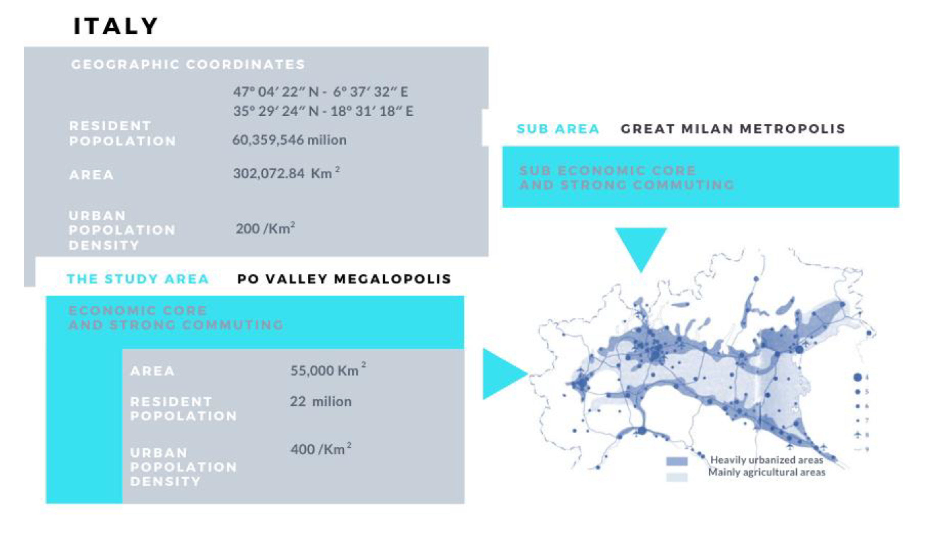
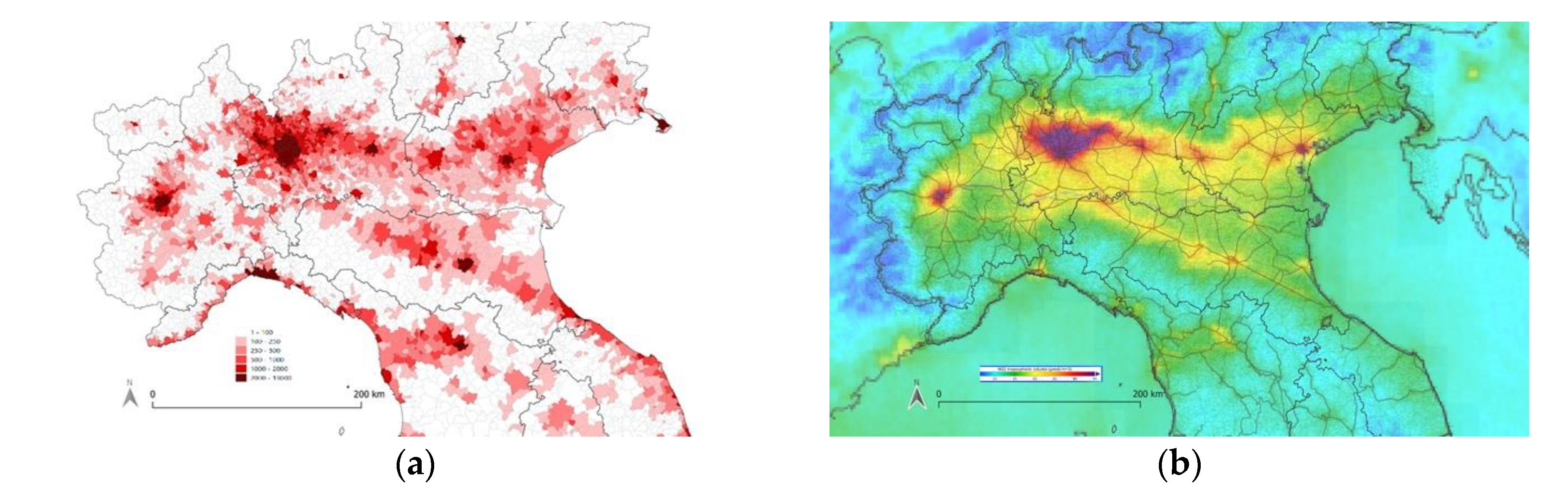
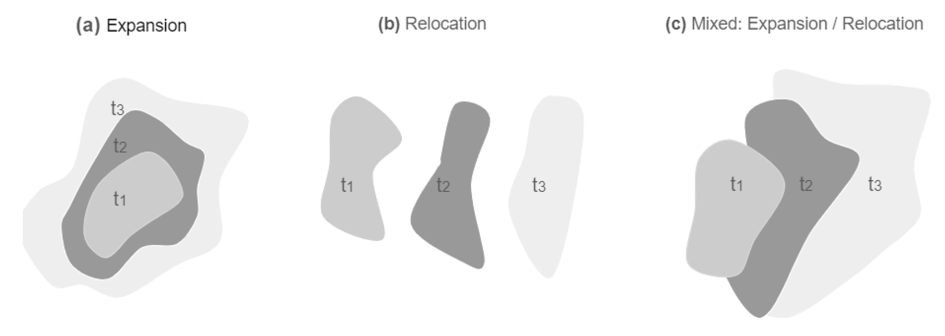
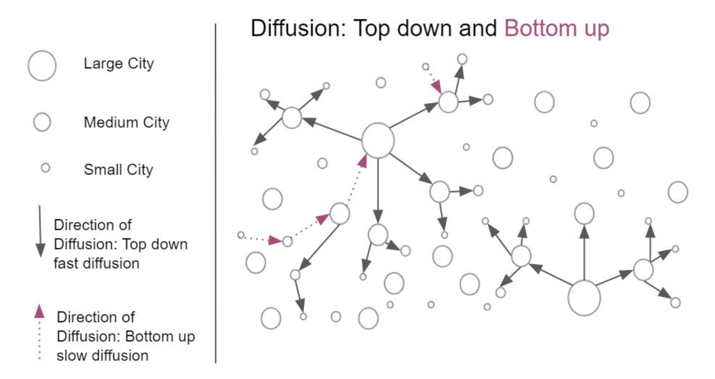
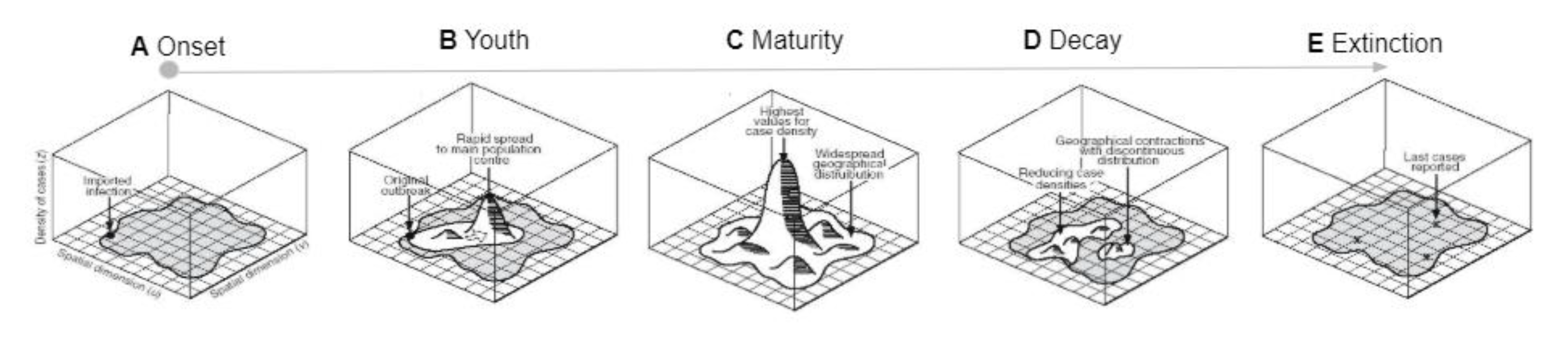
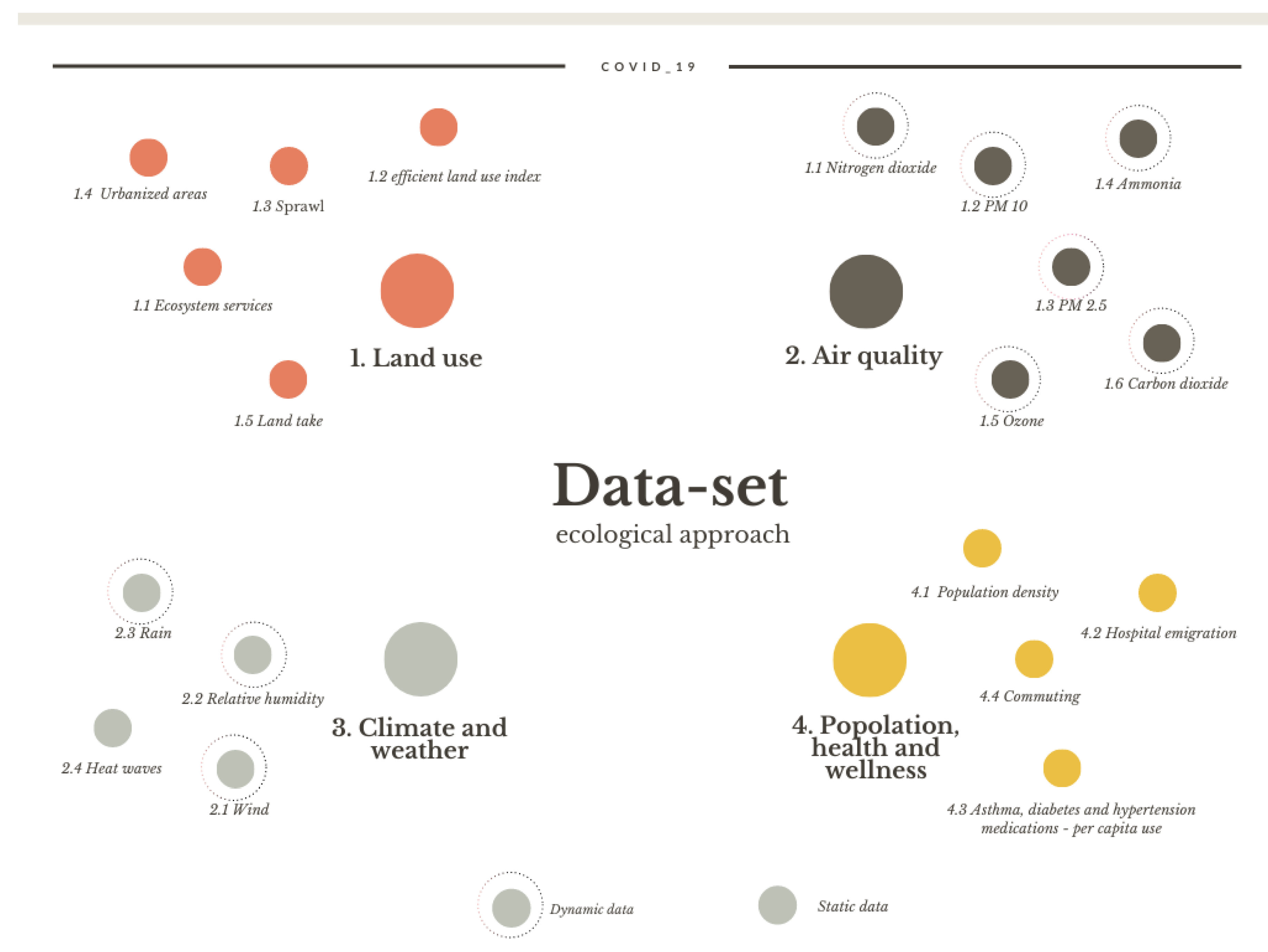
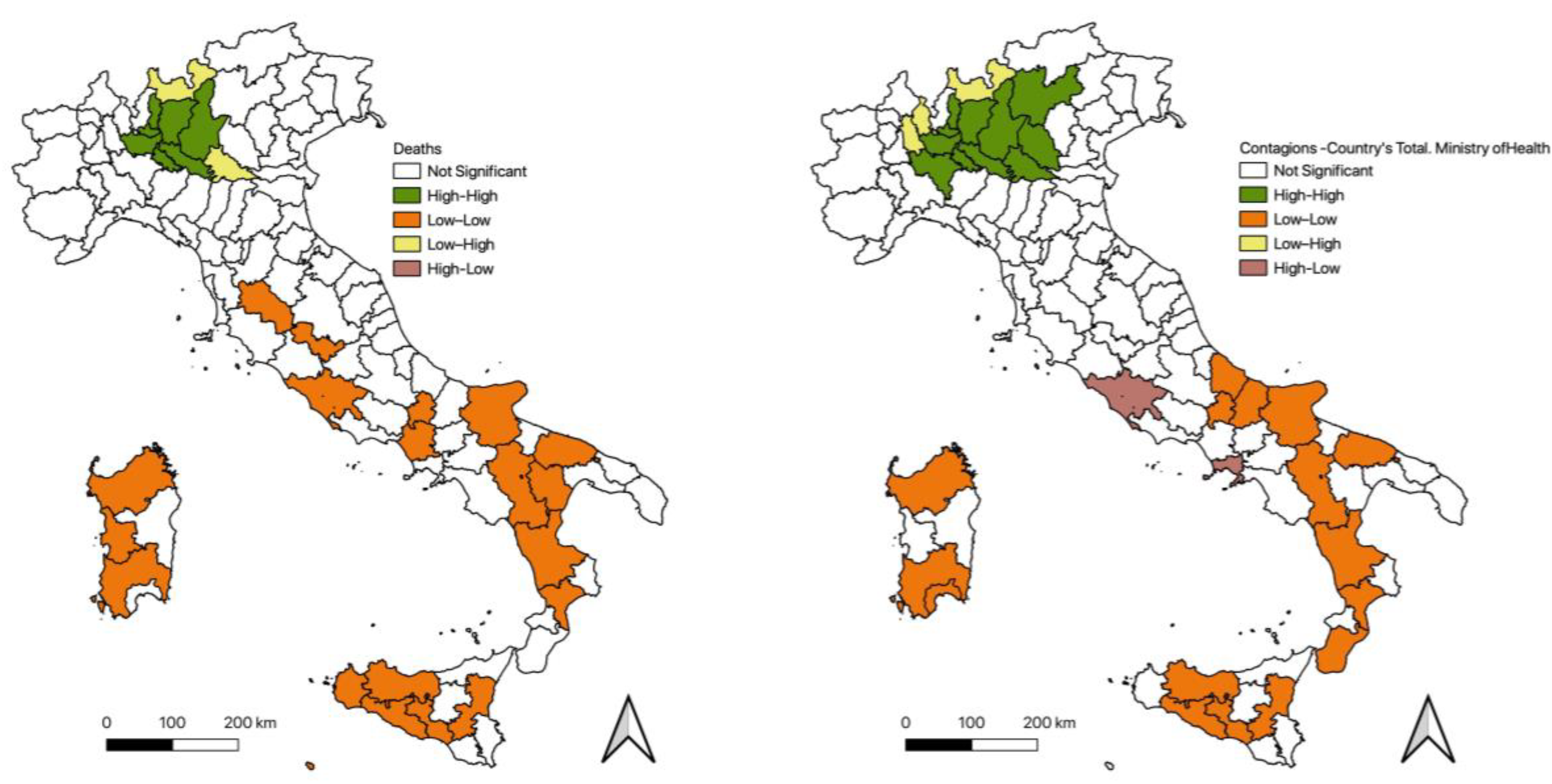
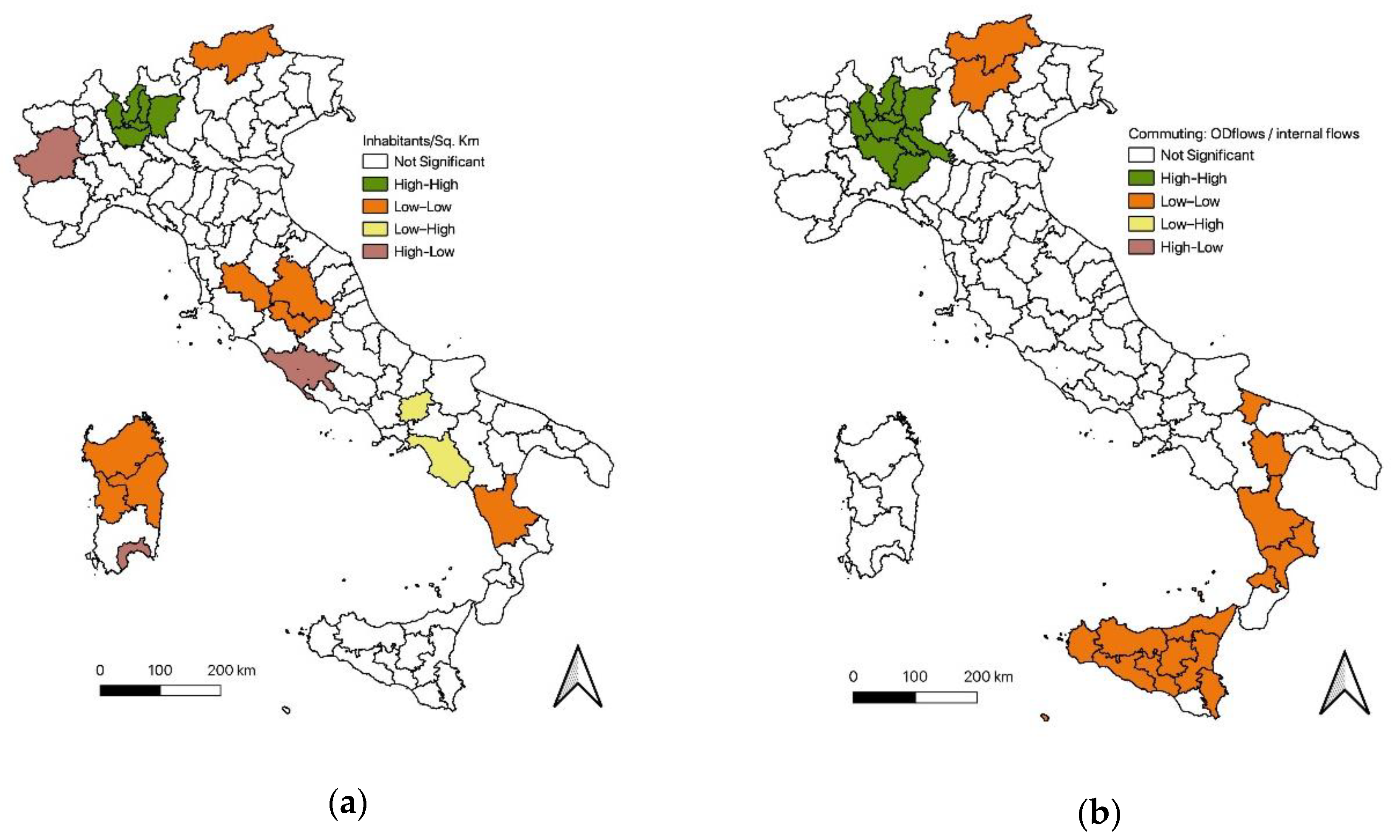
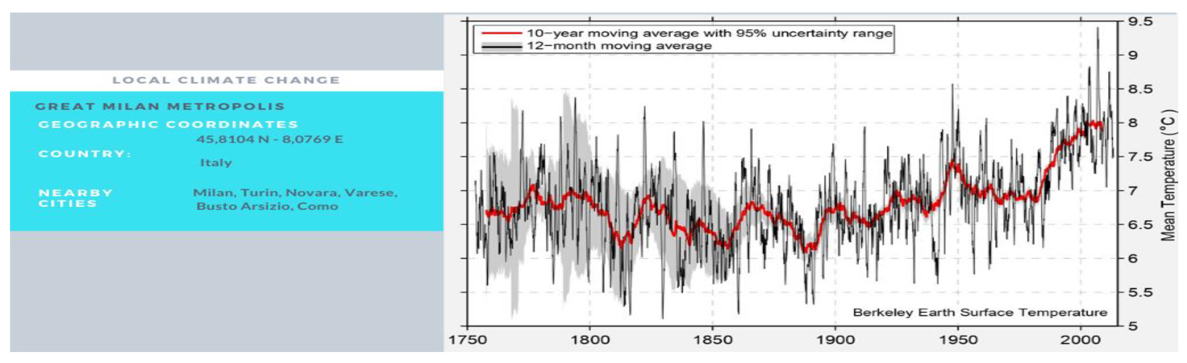
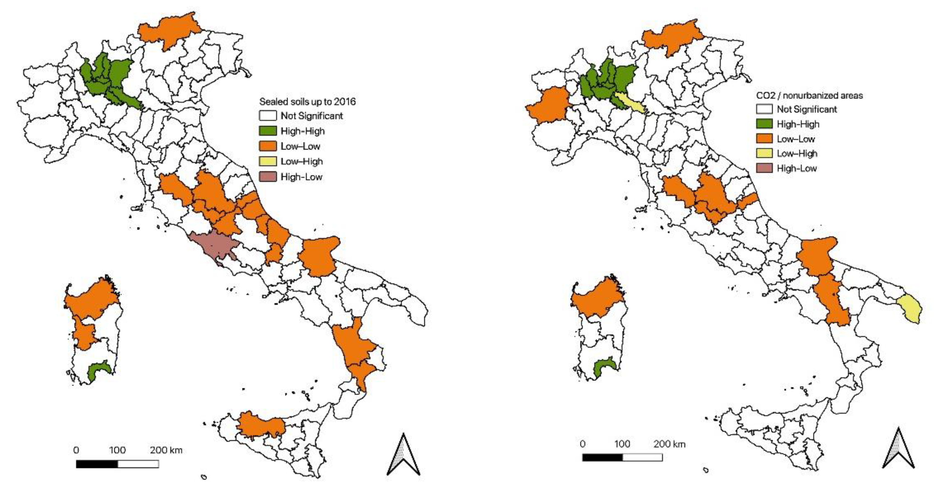
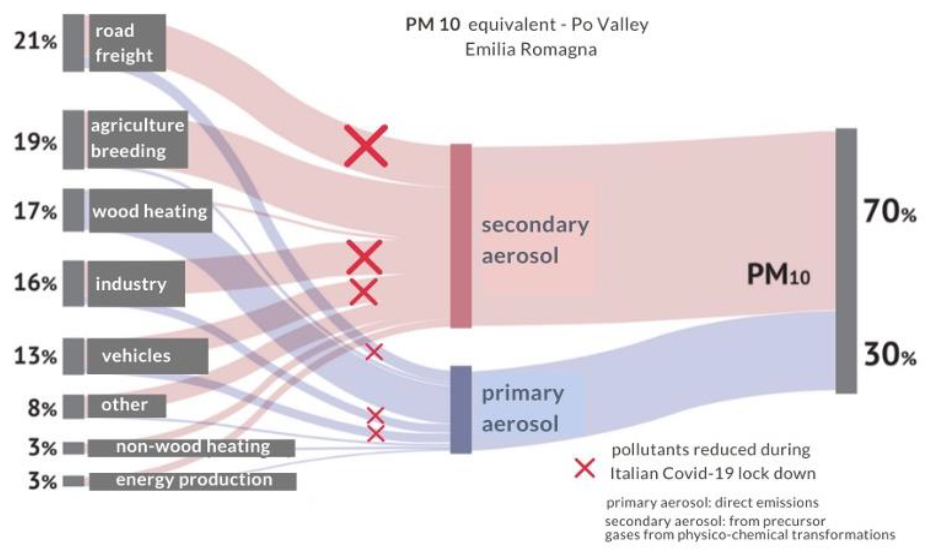
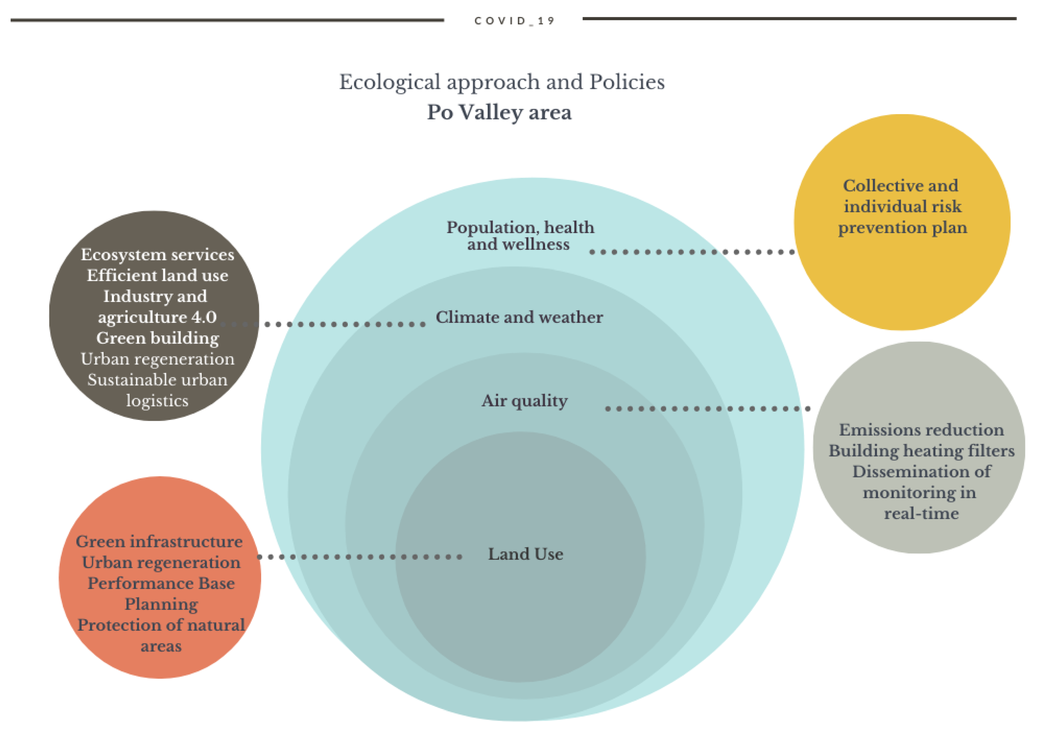
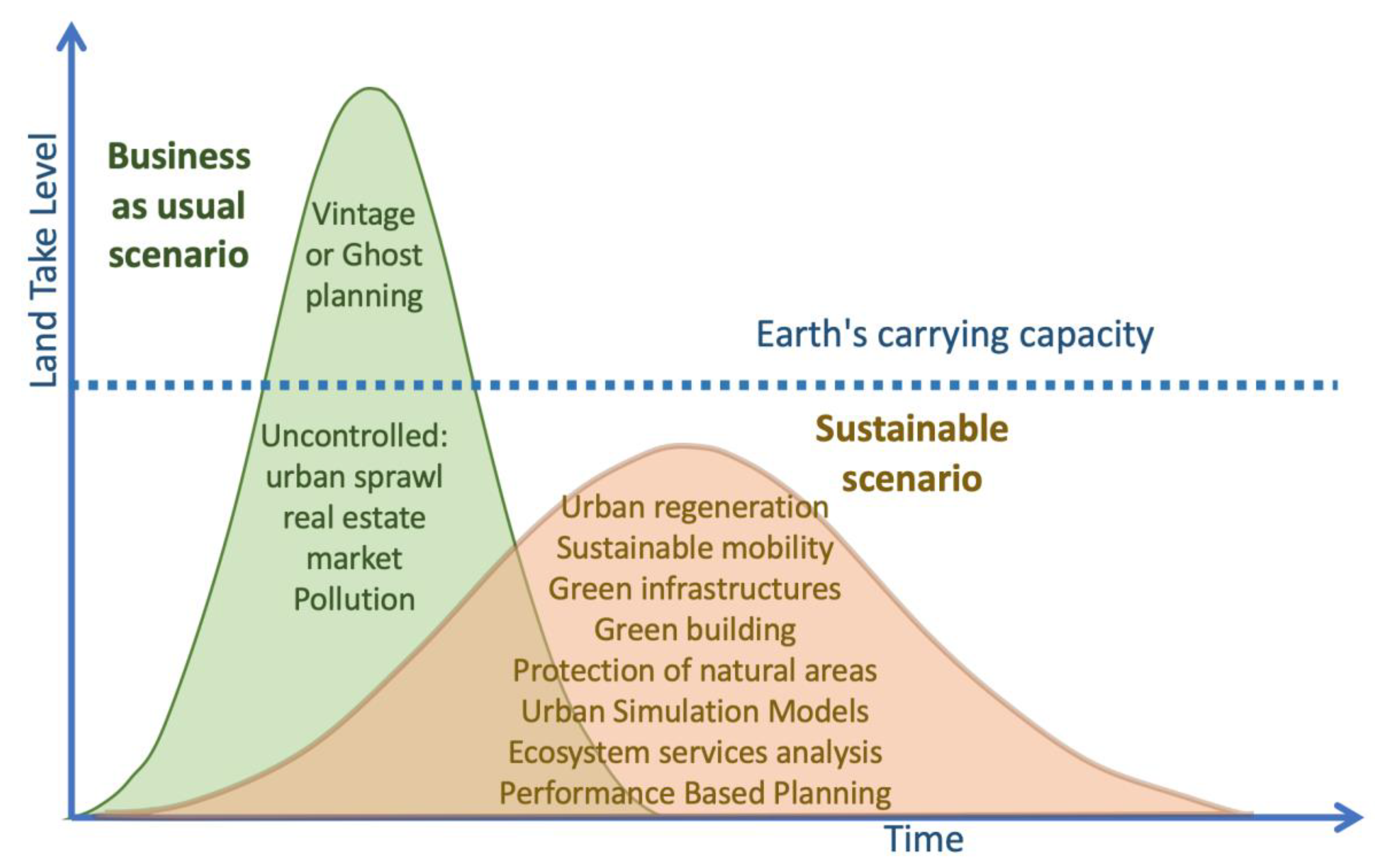
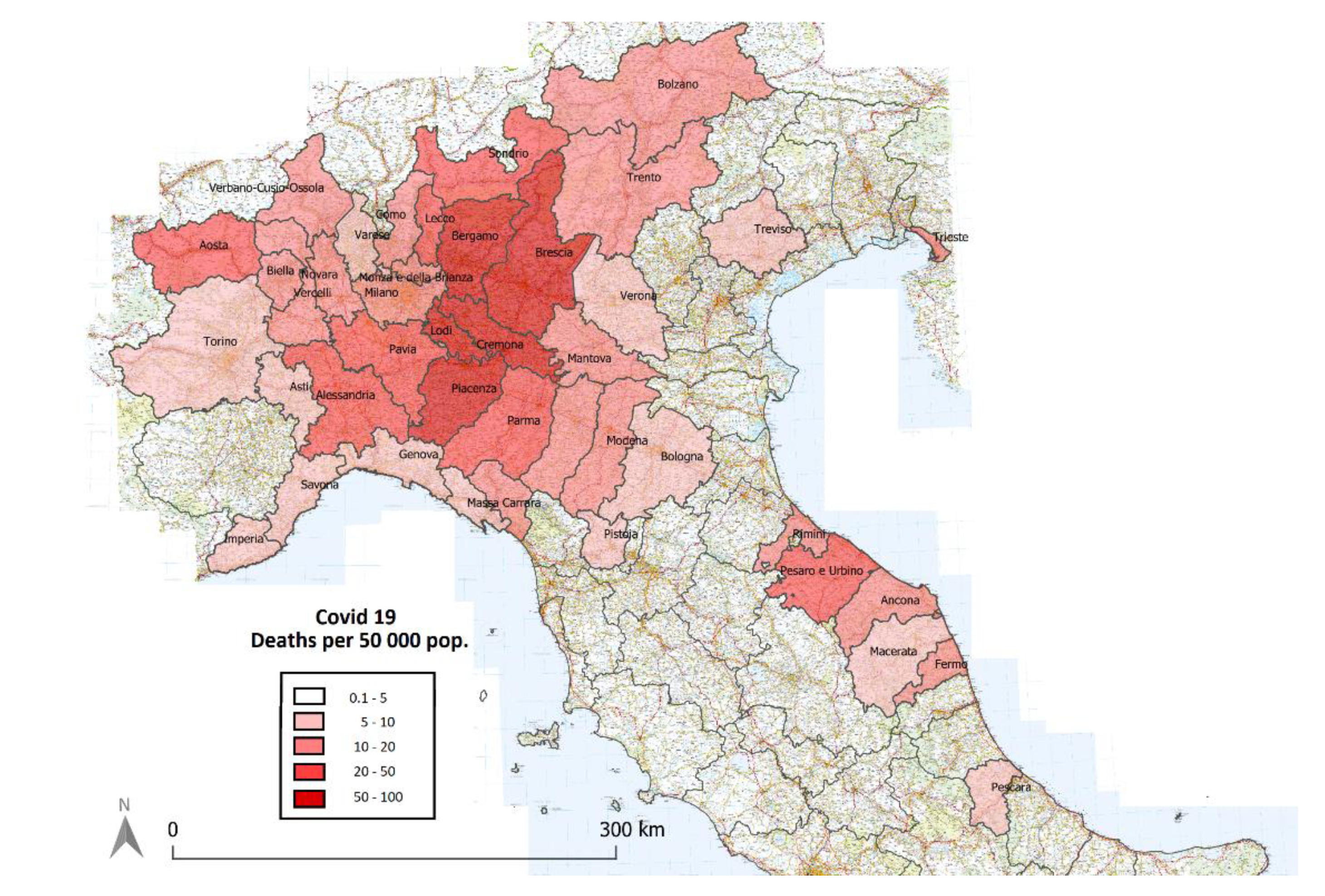
Table A1.
Data and indicators used in the LISA.
| Data/Index | Cov_ | Source | Data Origin | Unit |
|---|---|---|---|---|
| Land take/Soil consumption 2019, total 2014-2018—ha/m2 | 3 | ISPRA 2019 | http://www.isprambiente.gov.it/it/temi/suolo-e-territorio/il-consumo-di-suolo/i-dati-sul-consumo-di-suolo | provincial |
| PM2.5—average yearly values—μg/mc | 14 | ISPRA 2019 | http://www.isprambiente.gov.it/ | urban/periurban |
| PM10—average yearly values—μg/mc | 15 | Il SOLE 24 Ore 2019 | https://lab24.ilsole24ore.com/qualita-della-vita/classifiche-complete.php | urban/periurban |
| Ozone (O3)—days exceeding mobile average on 8 h—120 μg/m3 | 19 | ISPRA 2019 | http://www.isprambiente.gov.it/it/temi/suolo-e-territorio/il-consumo-di-suolo/i-dati-sul-consumo-di-suolo | Urban/periurban |
| COVID-19-Infected | 20 | Ministry of Health (15 April 2020) | http://www.salute.gov.it/imgs/C_17_notizie_4370_1_file.pdf | provincial |
| Ammonia (NH3)—Mg | 25 | ISPRA 2017 | http://www.sinanet.isprambiente.it/it/sia-ispra/inventaria/disaggregazione-dellinventario-nazionale-2015/view | provincial |
| Hospital emigration | 33 | IL SOLE 24 Ore 2019 | https://lab24.ilsole24ore.com/qualita-della-vita/classifiche-complete.php | urban |
| Drugs per capita: asthma, diabetes and hypertension | 70 | IL SOLE 24 Ore 2019 | https://lab24.ilsole24ore.com/qualita-della-vita/classifiche-complete.php | urban |
| Climate well-being index | 37 | IL SOLE 24 Ore 2019 | https://lab24.ilsole24ore.com/indice-del-clima/ | |
| Wind gusts, annual days with gusts> 25 knots | 39 | IL SOLE 24 Ore 2019 | https://lab24.ilsole24ore.com/indice-del-clima/ | urban |
| Fog | 41 | IL SOLE 24 Ore 2019 | https://lab24.ilsole24ore.com/indice-del-clima/ | urban |
| Surface waterproofed to year 2016 | 49 | ISPRA 2019 | provincial | |
| Urbanized areas early 2000s | 52 | Papers By Romano et al. reported in references | ||
| Km/h wind—Il meteo.com Meteo archive—January–February–March 2020 | 55 | IL METEO.it (2020) | http://www.ilmeteo.it | Urban/periurban |
| COVID-19 Deaths | 57 | Different Sources (31 March 2020) | Provincial | |
| COVID-19 Infected | 58 | Ministry of Health (31 March 2020) | http://www.salute.gov.it/imgs/C_17_notizie_4370_1_file.pdf | Regional/provincial |
| Inhabitants/Km2 | 64 | ISTAT 2019 | http://demo.istat.it/pop2019/index3.html?fbclid=IwAR3ZfOAubR1OBU3xD5qvD5FKWMhKW9Cxy1KF68GCZMJxgnIy1SIe4MJlrEI | provincial |
| Lethality | 65 | Ministry of Health (31 March 2020) | http://www.salute.gov.it/imgs/C_17_notizie_4370_1_file.pdf | |
| SMR | 66 | Our elaboration/data from various sources; Ministry of Health | provincial | |
| PM10 + Ozone—overrun days 2017–2019 | 72 | Legambiente (2020) | https://www.legambiente.it/wp-content/uploads/2020/01/Malaria-di-citta-2020.pdf | provincial |
| CO2/non urbanized areas | 82 | |||
| Commuting: OD flows/internal flows | 83 | ISTAT 2011 (census data) | https://www.istat.it/pendolarismo/grafici_province_cartografia_2011.html | provincial |
Appendix B
Figure A1.
ESA Nitrogen dioxide pollution and selected areas.: (a) Hubei Province in China with Wuhan Metropolitan areas; (b) Italy and Administrative Regions. Lombardy (Top Centre) with highest level of pollution.
Figure A1.
ESA Nitrogen dioxide pollution and selected areas.: (a) Hubei Province in China with Wuhan Metropolitan areas; (b) Italy and Administrative Regions. Lombardy (Top Centre) with highest level of pollution.
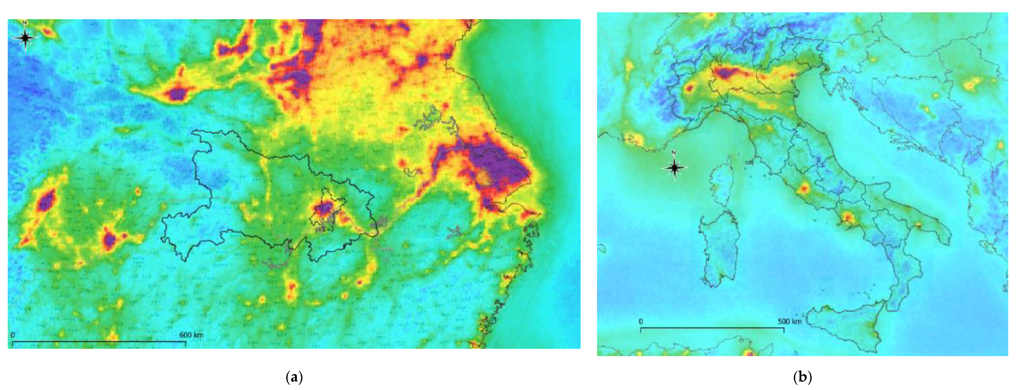
Figure A2.
(a) Population density in Italian Municipalities; (b) LISA map on Population density in Italian Municipalities. Source: Our elaborations from ISTAT population data 2019 (http://demo.istat.it).
Figure A2.
(a) Population density in Italian Municipalities; (b) LISA map on Population density in Italian Municipalities. Source: Our elaborations from ISTAT population data 2019 (http://demo.istat.it).
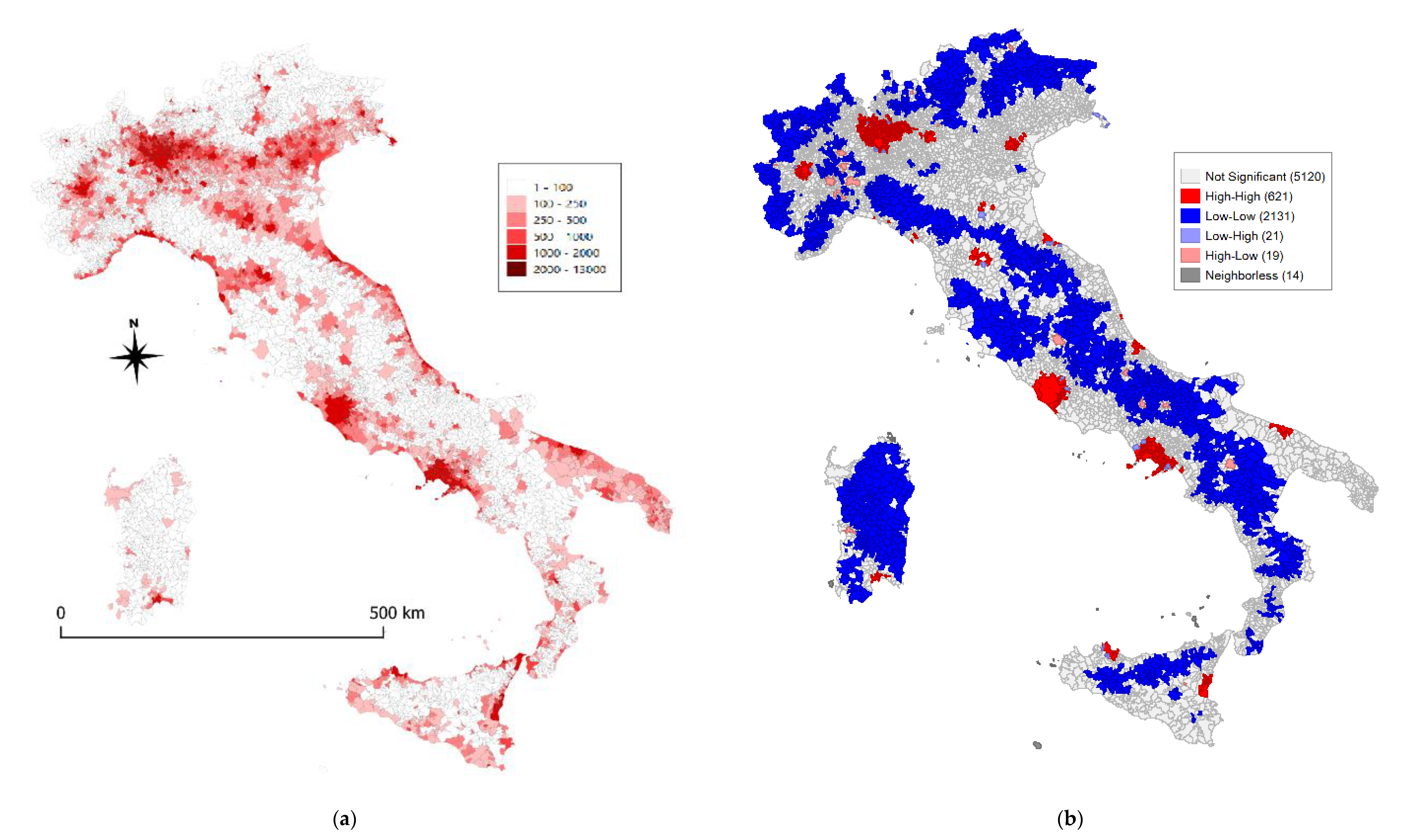
Figure A3.
Deaths per 50,000 inhabitants. Focus on Po Valley Area. Source: our elaboration from COVID-19 data originally collected; ISTAT 2019 (population).
Figure A3.
Deaths per 50,000 inhabitants. Focus on Po Valley Area. Source: our elaboration from COVID-19 data originally collected; ISTAT 2019 (population).

Figure A4.
Population density. Inhabitants/Km2. Focus on the Po Valley Area. Source: our elaboration from data originally collected; ISTAT 2019.
Figure A4.
Population density. Inhabitants/Km2. Focus on the Po Valley Area. Source: our elaboration from data originally collected; ISTAT 2019.
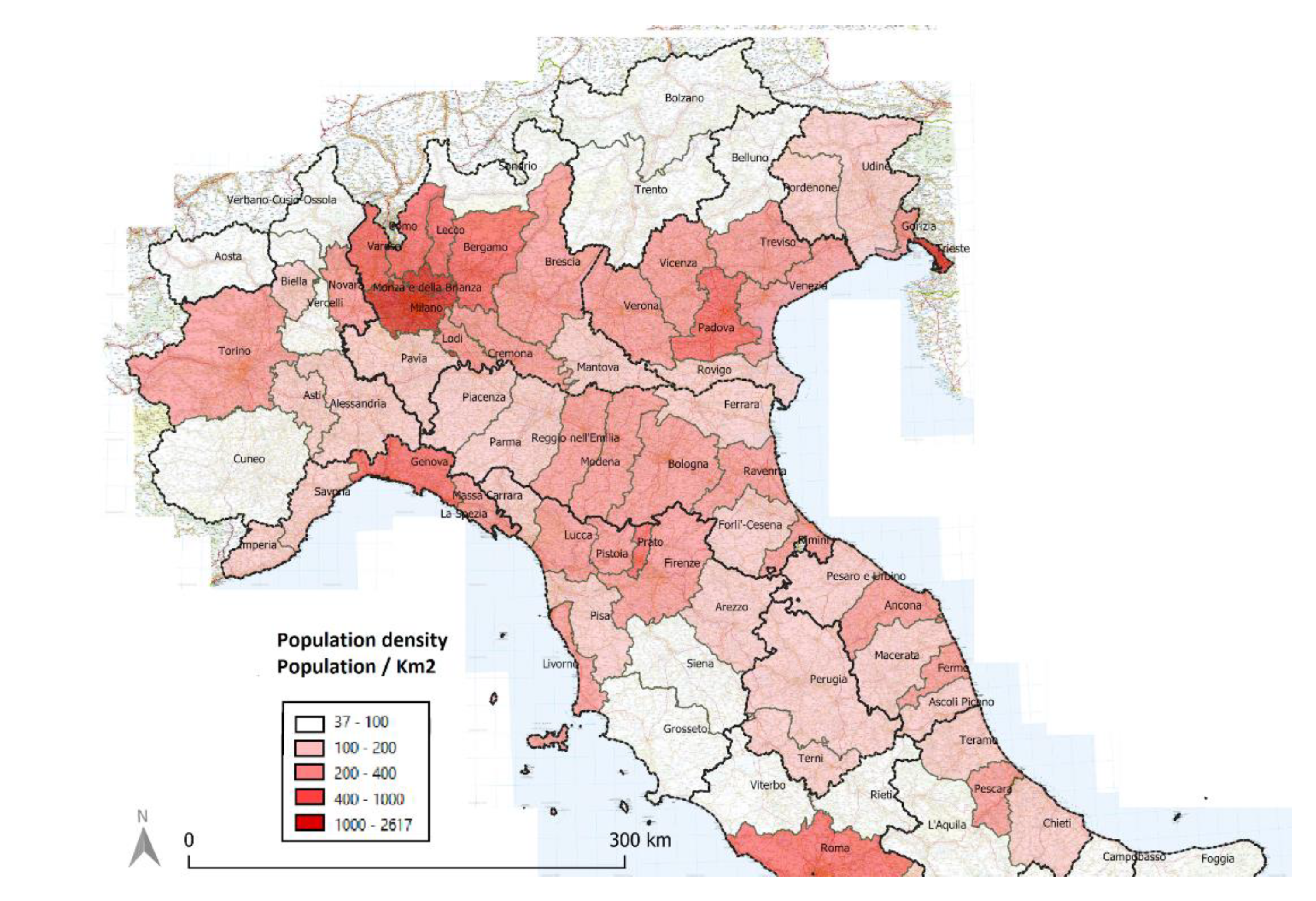
References
- Gorbalenya, A.E.; Baker, S.C.; Baric, R.S.; de Groot, R.J.; Drosten, C.; Gulyaeva, A.A.; Haagmans, B.L.; Lauber, C.; Leontovich, A.M.; Neuman, B.W.; et al. The species Severe acute respiratory syndrome-related coronavirus: Classifying 2019-nCoV and naming it SARS-CoV-2. Nat. Microbiol. 2020, 5, 536–544. [Google Scholar]
- World Health Organization. Coronavirus Disease 2019 (COVID-19) Situation Report-92; World Health Organization: Geneva, Switzerland, 2020. [Google Scholar]
- World Health Organization. Report of the WHO-China Joint Mission on Coronavirus Disease 2019 (COVID-19); World Health Organization: Geneva, Switzerland, 2020. [Google Scholar]
- World Health Organization. Coronavirus Disease 2019 (COVID-19) Situation Report-12; World Health Organization: Geneva, Switzerland, 2020. [Google Scholar]
- Istituto Superiore della Sanità. Report Sulle Caratteristiche dei Pazienti Deceduti Positivi a COVID-19 in Italia Report Basato su dati Aggiornati al 20 Marzo 2020; Istituto Superiore della Sanità: Roma, Italy, 2020. [Google Scholar]
- Istituto Superiore della Sanità. Epidemia COVID-19; Istituto Superiore della Sanità: Roma, Italy, 2020. [Google Scholar]
- Eurostat Population Structure and Ageing. Available online: https://ec.europa.eu/eurostat/statistics-explained/index.php/Population_structure_and_ageing (accessed on 19 April 2020).
- Istituto Cattaneo. La Crescita della Mortalità ai Tempi del Covid-19 Analisi di 1.084 Comuni Italiani; Istituto Cattaneo: Bologna BO, Italy, 2020. [Google Scholar]
- Istituto Nazionale di Statistica. Anziani: Le condizioni di salute in Italia e nell’Unione Europea; Istituto Nazionale di Statistica: Rome, Italy, 2015. [Google Scholar]
- Gurwitz, D. Angiotensin receptor blockers as tentative SARS-CoV-2 therapeutics. Drug Dev. Res. 2020, 21656. [Google Scholar] [CrossRef] [PubMed] [Green Version]
- Agenzia Italiana del Farmaco. Precisazioni AIFA su Malattia da Coronavirus Covid-19 ed Utilizzo di ACE-INIBITORI E SARTANI; Agenzia Italiana del Farmaco: Rome, Italy, 2020. [Google Scholar]
- Rothe, C.; Schunk, M.; Sothmann, P.; Bretzel, G.; Froeschl, G.; Wallrauch, C.; Zimmer, T.; Thiel, V.; Janke, C.; Guggemos, W.; et al. Transmission of 2019-NCOV infection from an asymptomatic contact in Germany. N. Engl. J. Med. 2020, 382, 970–971. [Google Scholar] [CrossRef] [Green Version]
- Van Doremalen, N.; Bushmaker, T.; Morris, D.H.; Holbrook, M.G.; Gamble, A.; Williamson, B.N.; Tamin, A.; Harcourt, J.L.; Thornburg, N.J.; Gerber, S.I.; et al. Aerosol and Surface Stability of SARS-CoV-2 as Compared with SARS-CoV-1. N. Engl. J. Med. 2020. [Google Scholar] [CrossRef]
- Peng, L.; Zhao, X.; Tao, Y.; Mi, S.; Huang, J.; Zhang, Q. The effects of air pollution and meteorological factors on measles cases in Lanzhou, China. Environ. Sci. Pollut. Res. 2020, 27, 13524–13533. [Google Scholar] [CrossRef]
- Chen, J.-C.; Schwartz, J. Metabolic Syndrome and Inflammatory Responses to Long-Term Particulate Air Pollutants. Environ. Health Perspect. 2008, 116, 612–617. [Google Scholar] [CrossRef] [Green Version]
- Conticini, E.; Frediani, B.; Caro, D. Can atmospheric pollution be considered a co-factor in extremely high level of SARS-CoV-2 lethality in Northern Italy? Environ. Pollut. 2020, 261, 114465. [Google Scholar] [CrossRef]
- Mandhana, N.; Solomon, F. Business Meeting at Luxury Singapore Hotel Becomes Latest Coronavirus Focus. Wall Str. J. 2020. [Google Scholar]
- European Space Agency COVID-19: Nitrogen Dioxide Over China. Available online: https://www.esa.int/Applications/Observing_the_Earth/Copernicus/Sentinel-5P/COVID-19_nitrogen_dioxide_over_China (accessed on 22 April 2020).
- European Space Agency Coronavirus: Nitrogen Dioxide Emissions Drop over Italy. Available online: http://www.esa.int/ESA_Multimedia/Videos/2020/03/Coronavirus_nitrogen_dioxide_emissions_drop_over_Italy (accessed on 22 April 2020).
- Skarbit, N.; Ács, F.; Breuer, H. The climate of the European region during the 20th and 21st centuries according to Feddema. Int. J. Climatol. 2018, 38, 2435–2448. [Google Scholar] [CrossRef]
- Huang, Y.; Lu, S.; Yang, X.; Zhao, Z. Exploring Railway Network Dynamics in China from 2008 to 2017. ISPRS Int. J. Geo-Inf. 2018, 7, 320. [Google Scholar] [CrossRef] [Green Version]
- Yu, Y.; He, J.; Tang, W.; Li, C. Modeling Urban Collaborative Growth Dynamics Using a Multiscale Simulation Model for the Wuhan Urban Agglomeration Area, China. ISPRS Int. J. Geo-Inf. 2018, 7, 176. [Google Scholar] [CrossRef] [Green Version]
- Assaeroporti Dati Annuali Traffico Aeroportuale Italiano. Available online: https://assaeroporti.com/dati-annuali/ (accessed on 22 April 2020).
- Romano, B.; Zullo, F.; Fiorini, L.; Marucci, A.; Ciabò, S. Land transformation of Italy due to half a century of urbanization. Land Use Policy 2017, 67, 387–400. [Google Scholar] [CrossRef]
- Pezzagno, M.; Richiedei, A.; Tira, M. Spatial Planning Policy for Sustainability: Analysis Connecting Land Use and GHG Emission in Rural Areas. Sustainability 2020, 12, 947. [Google Scholar] [CrossRef] [Green Version]
- Senes, G.; Fumagalli, N.; Ferrario, P.; Rovelli, R.; Sigon, R. Definition of a Land Quality Index to preserve the best territories from future land take. An application to a study area in Lombardy (Italy). J. Agric. Eng. 2020, 51, 43–55. [Google Scholar] [CrossRef]
- Lu, X.; Chen, D.; Wang, Y. Is urban sprawl decoupled from the quality of economic growth? Evidence from Chinese cities. Sustainability 2020, 12, 218. [Google Scholar] [CrossRef] [Green Version]
- Setti, L.; Rizzo-Società, E.; Medicina, I.; Alessandro, A.; Italiana, M.-S.; Ambientale, M. Relazione Circa L’effetto Dell’inquinamento da Particolato Atmosferico e la Diffusione di Virus Nella Popolazione; Università di Bologna: Bologna, Italy, 2020. [Google Scholar]
- Du, Z.; Lawrence, W.R.; Zhang, W.; Zhang, D.; Yu, S.; Hao, Y. Interactions between climate factors and air pollution on daily HFMD cases: A time series study in Guangdong, China. Sci. Total Environ. 2019, 656, 1358–1364. [Google Scholar] [CrossRef]
- Roussel, I. Extreme Weather Events and Air Pollution Peaks in the Light of Climate Change: The Limits of the Notion of Risk. In Extreme Weather Events and Human Health; Akhtar, R., Ed.; Springer International Publishing: Berlin/Heidelberg, Germany, 2020; pp. 59–78. ISBN 978-3-030-23772-1. [Google Scholar]
- Jacob, D.J.; Winner, D.A. Effect of climate change on air quality. Atmos. Environ. 2009, 43, 51–63. [Google Scholar] [CrossRef] [Green Version]
- Maione, M.; Fowler, D.; Monks, P.S.; Reis, S.; Rudich, Y.; Williams, M.L.; Fuzzi, S. Air quality and climate change: Designing new win-win policies for Europe. Environ. Sci. Policy 2016, 65, 48–57. [Google Scholar] [CrossRef] [Green Version]
- European Environment Agency. Europes Urban Air Quality—Re-Assessing Implementation Challenges in Cities—European Environment Agency EEA Report No 24/2018; European Environment Agency: København, Denmark, 2018. [Google Scholar]
- European Environment. Agency Air quality and COVID-19—European Environment Agency; European Environment Agency: København, Denmark, 2020. [Google Scholar]
- Reames, T.G.; Bravo, M.A. People, place and pollution: Investigating relationships between air quality perceptions, health concerns, exposure, and individual- and area-level characteristics. Environ. Int. 2019, 122, 244–255. [Google Scholar] [CrossRef]
- Mitsakou, C.; Dimitroulopoulou, S.; Heaviside, C.; Katsouyanni, K.; Samoli, E.; Rodopoulou, S.; Costa, C.; Almendra, R.; Santana, P.; Dell’Olmo, M.M.; et al. Environmental public health risks in European metropolitan areas within the EURO-HEALTHY project. Sci. Total Environ. 2019, 658, 1630–1639. [Google Scholar] [CrossRef]
- Chalvatzaki, E.; Chatoutsidou, S.E.; Lehtomäki, H.; Almeida, S.M.; Eleftheriadis, K.; Hänninen, O.; Lazaridis, M. Characterization of human health risks from particulate air pollution in selected European cities. Atmosphere 2019, 10, 96. [Google Scholar] [CrossRef] [Green Version]
- Sofia, D.; Gioiella, F.; Lotrecchiano, N.; Giuliano, A. Mitigation strategies for reducing air pollution. Environ. Sci. Pollut. Res. 2020, 1–10. [Google Scholar] [CrossRef] [PubMed]
- Magnani, N.; Carrosio, G.; Osti, G. Energy retrofitting of urban buildings: A socio-spatial analysis of three mid-sized Italian cities. Energy Policy 2020, 139, 111341. [Google Scholar] [CrossRef]
- Legambiente. Mal’aria di Città; Legambiente: Rome, Italy, 2020. [Google Scholar]
- Blum, J. Contribution of Ecosystem Services to Air Quality and Climate Change Mitigation Policies: The Case of Urban Forests in Barcelona, Spain. In Urban Forests Ecosystem Services and Management; Blum, J., Ed.; Apple Academic Press: New York, NY, USA, 2017; pp. 21–54. ISBN 9781315366081. [Google Scholar]
- Regione Lombardia. Piano Aria Regione Lombardia—Comune di Milano; Regione Lombardia: Milan, Italy, 2018. [Google Scholar]
- Regione Emilia-Romagna. Piano Aria Integrato Regionale (PAIR 2020) dell’Emilia-Romagna; Regione Emilia-Romagna: Bologna, Italy, 2020. [Google Scholar]
- Turri, E. La Megalopoli Padana; Marsilio Editori: Venice, Italy, 2001; ISBN 978-88-317-7556-4. [Google Scholar]
- Brunet, R. Les Villes “Européennes”; La Documentation Française: Paris, France, 1989; ISBN 9782110022004. [Google Scholar]
- AA. VV. Megalopoli Mediterranea. | 598; Muscarà, C., Ed.; FrancoAngeli: Milan, Italy, 1978. [Google Scholar]
- Dematteis, G. Il Fenomeno Urbano in Italia; DeMatteis, G., Ed.; FrancoAngeli: Milan, Italy, 1992. [Google Scholar]
- Boeri, S.; Lanzani, A.; Marini, E. Il Territorio Che Cambia: Ambienti, Paesaggi e Immagini Della Regione Milanese; Abitare Segesta: Lombardy, Italy, 1993; ISBN 8886116179. [Google Scholar]
- Boscacci, F.; Camagni, R. Tra Città e Campagna: Periurbanizzazione e Politiche Territoriali; Il Mulino: Bologna, Italy, 1994; ISBN 8815047816. [Google Scholar]
- Turri, E. Il Paesaggio Degli Uomini: La Natura, la Cultura, la Storia; Zanichelli: Bologna, Italy, 2003; ISBN 9788808072337. [Google Scholar]
- Turco, A. Governance territoriale. Norme, Discorsi, Pratiche; Unicopli: Milan, Italy, 2013; ISBN 9788840016344. [Google Scholar]
- Turco, A. Paesaggio, Luogo, Ambiente. La Configuratività Territoriale Come Bene Comune—A. Turco—Libro—Studi e Ricerche Sul Territorio | IBS; Unicopli: Milan, Italy, 2014; ISBN 9788840017181. [Google Scholar]
- Dagradi, P. PADANA, PIANURA. Encicl. Ital. Treccani Appendice 1994. [Google Scholar]
- ARPA Lombardia. Indice di Qualità Dell’aria—Aria / Qualità dell’Aria; ARPA Lombardia: Milan, Italy, 2019. [Google Scholar]
- ARPA Veneto. QUALITÀ DELL’ARIA—DATI VALIDATI; ARPA Veneto: Padua, Italy, 2019. [Google Scholar]
- European Environment Agency. Urban Sprawl in Europe—The Ignored Challenge—European Environment Agency; European Environment Agency: Luxembourg, 2006. [Google Scholar]
- Romano, B.; Zullo, F. The urban transformation of Italy’s Adriatic coastal strip: Fifty years of unsustainability. Land Use Policy 2014, 38, 26–36. [Google Scholar] [CrossRef]
- Romano, B.; Zullo, F. Half a century of urbanization in southern European lowlands: A study on the Po Valley (Northern Italy). Urban Res. Pract. 2016, 9, 109–130. [Google Scholar] [CrossRef]
- Romano, B.; Zullo, F. Land urbanization in Central Italy: 50 years of evolution. J. Land Use Sci. 2014, 9, 143–164. [Google Scholar] [CrossRef]
- Geneletti, D. Assessing the impact of alternative land-use zoning policies on future ecosystem services. Environ. Impact Assess. Rev. 2013, 40, 25–35. [Google Scholar] [CrossRef]
- Geneletti, D. Ecosystem services for Strategic Environmental Assessment: Concepts and examples. In Handbook on Biodiversity and Ecosystem Services in Impact Assessment; Geneletti, D., Ed.; Edward Elgar Publishing: Cheltenham, UK, 2016; pp. 41–61. ISBN 978 1 78347 898 9. [Google Scholar]
- Sallustio, L.; Munafò, M.; Riitano, N.; Lasserre, B.; Fattorini, L.; Marchetti, M. Integration of land use and land cover inventories for landscape management and planning in Italy. Environ. Monit. Assess. 2016, 188, 1–20. [Google Scholar] [CrossRef]
- European Commission. Guidelines on Best Practice to Limit, Mitigate or Compensate Soil Sealing. European Commission: Bruxelles, Belgium, 2012. [Google Scholar]
- Munafò, M.; Salvati, L.; Zitti, M. Estimating soil sealing rate at national level—Italy as a case study. Ecol. Indic. 2013, 26, 137–140. [Google Scholar] [CrossRef]
- Lawler, J.J.; Lewis, D.J.; Nelson, E.; Plantinga, A.J.; Polasky, S.; Withey, J.C.; Helmers, D.P.; Martinuzzi, S.; Penningtonh, D.; Radeloff, V.C. Projected land-use change impacts on ecosystem services in the United States. Proc. Natl. Acad. Sci. USA 2014, 111, 7492–7497. [Google Scholar] [CrossRef] [PubMed] [Green Version]
- Geneletti, D.; Biasiolli, A.; Morrison-Saunders, A. Land take and the effectiveness of project screening in Environmental Impact Assessment: Findings from an empirical study. Environ. Impact Assess. Rev. 2017, 67, 117–123. [Google Scholar] [CrossRef]
- Zomer, R.J.; Bossio, D.A.; Sommer, R.; Verchot, L.V. Global Sequestration Potential of Increased Organic Carbon in Cropland Soils. Sci. Rep. 2017, 7, 1–8. [Google Scholar] [CrossRef] [PubMed] [Green Version]
- Manes, F.; Marando, F.; Capotorti, G.; Blasi, C.; Salvatori, E.; Fusaro, L.; Ciancarella, L.; Mircea, M.; Marchetti, M.; Chirici, G.; et al. Regulating Ecosystem Services of forests in ten Italian Metropolitan Cities: Air quality improvement by PM10 and O3 removal. Ecol. Indic. 2016, 67, 425–440. [Google Scholar] [CrossRef]
- Fusaro, L.; Marando, F.; Sebastiani, A.; Capotorti, G.; Blasi, C.; Copiz, R.; Congedo, L.; Munafò, M.; Ciancarella, L.; Manes, F. Mapping and Assessment of PM10 and O3 Removal by Woody Vegetation at Urban and Regional Level. Remote Sens. 2017, 9, 791. [Google Scholar] [CrossRef] [Green Version]
- Salvati, L.; Munafo, M.; Morelli, V.G.; Sabbi, A. Low-density settlements and land use changes in a Mediterranean urban region. Landsc. Urb. Plan. 2012, 105, 43–52. [Google Scholar] [CrossRef]
- Romano, B.; Zullo, F.; Fiorini, L.; Ciabò, S.; Marucci, A. Sprinkling: An Approach to Describe Urbanization Dynamics in Italy. Sustainability 2017, 9, 97. [Google Scholar] [CrossRef] [Green Version]
- Saganeiti, L.; Favale, A.; Pilogallo, A.; Scorza, F.; Murgante, B. Assessing urban fragmentation at regional scale using sprinkling indexes. Sustainability 2018, 10, 3274. [Google Scholar] [CrossRef] [Green Version]
- Camagni, R.; Gibelli, M.C.; Rigamonti, P. Urban mobility and urban form: The social and environmental costs of different patterns of urban expansion. Ecol. Econ. 2002, 40, 199–216. [Google Scholar] [CrossRef]
- Manganelli, B.; Murgante, B.; Saganeiti, L. The Social Cost of Urban Sprinkling. Sustainability 2020, 12, 2236. [Google Scholar] [CrossRef] [Green Version]
- Hagerstrand, T. Innovation Diffusion as a Spatial Process; The University of Chicago Press: Chicago, IL, USA; London, UK, 1967. [Google Scholar]
- Gould, P.R. Spatial Diffusion. In Association of American Geographers; Association of American Geographers: Washington, DC, USA, 1969. [Google Scholar]
- Morrill, R.L. The Shape of Diffusion in Space and Time. Econ. Geogr. 1970, 46, 259. [Google Scholar] [CrossRef]
- Morrill, R. Hägerstrand and the ‘quantitative revolution’: A personal appreciation. Prog. Hum. Geogr. 2005, 29, 333–336. [Google Scholar] [CrossRef] [Green Version]
- FlightConnections—All flights worldwide on a map! Available online: https://www.flightconnections.com/ (accessed on 26 April 2020).
- Cliff, A.D.; Haggett, P. A swash-backwash model of the single epidemic wave. J. Geogr. Syst. 2006, 8, 227–252. [Google Scholar] [CrossRef] [PubMed] [Green Version]
- Haggett, P.; Cliff, A. The Geography of Disease Distributions. In A Century of British Geography. Johnston, R., Williams, M., Eds.; Oxford University Press: Oxford, UK, 2003; pp. 521–543. ISBN 0197262864. [Google Scholar]
- Haggett, P.; Cliff, A. Modeling diffusion processes. In Encyclopaedia of Social Measurement; Kempf-Leonard, K., Ed.; Elsevier Ltd.: Amsterdam, The Netherlands, 2005; Volume 2, pp. 709–724. ISBN 0124366430. [Google Scholar]
- Matthew, S.-R.; Peter, H.; Andrew, C. World Atlas of Epidemic Diseases; CRC Press: Boca Raton, FL, USA, 2004; ISBN 9780429072499. [Google Scholar]
- Cliff, A.; Haggett, P.; Smallman-Raynor, M. Deciphering Global Epidemics; Cambridge University Press: Cambridge, UK, 1998. [Google Scholar]
- Cliff, A.D.; Haggett, P.; Smallman-Raynor, M. An exploratory method for estimating the changing speed of epidemic waves from historical data. Int. J. Epidemiol. 2008, 37, 106–112. [Google Scholar] [CrossRef] [Green Version]
- Haggett, P. Geography:A Global Synthesis; Hall, P., Ed.; Pearson Education: London, UK, 2001. [Google Scholar]
- Cliff, A.D.; Andrew, D.; Haggett, P.; Smallman-Raynor, M. Island Epidemics. Oxford University Press: Oxford, UK, 2000; ISBN 9780198288954. [Google Scholar]
- Tatem, A.J.; Rogers, D.J.; Hay, S.I. Global Transport Networks and Infectious Disease Spread. Adv. Parasitol. 2006, 62, 293–343. [Google Scholar] [CrossRef]
- Ben-Zion, Y.; Cohen, Y.; Shnerb, N.M. Modeling epidemics dynamics on heterogenous networks. J. Theor. Biol. 2010, 264, 197–204. [Google Scholar] [CrossRef]
- Bowen, J.T., Jr.; Laroe, C. Airline Networks and the International Diffusion of Severe Acute Respiratory Syndrome. Geogr. J. 2006, 172, 130–144. [Google Scholar] [CrossRef]
- Brockmann, D.; Helbing, D. The hidden geometry of complex, network-driven contagion phenomena. Science 2013, 342, 1337–1342. [Google Scholar] [CrossRef] [Green Version]
- Zhang, L.; Wilson, D.P. Trends in Notifiable Infectious Diseases in China: Implications for Surveillance and Population Health Policy. PLoS ONE 2012, 7, e31076. [Google Scholar] [CrossRef]
- Direct Flights from Wuhan (WUH). Available online: https://www.flightconnections.com/flights-from-wuhan-wuh (accessed on 28 April 2020).
- Eurostat. Energy and Transport in Figures; Eurostat: Luxembourg, 2019. [Google Scholar]
- Borruso, G. A nodal regional analysis of air passenger transport in Europe. Int. J. Bus. Intell. Data Min. 2013, 8, 377–396. [Google Scholar] [CrossRef]
- Koch-Institut, R. Epidemiologisches Bulletin FSME; Risikogebiete in Deutschland: Berlin, Germany, 2020. [Google Scholar]
- Backer, J.A.; Klinkenberg, D.; Wallinga, J. Incubation period of 2019 novel coronavirus (2019-nCoV) infections among travellers from Wuhan, China, 20–28 January 2020. Eurosurveillance 2020, 25, 2000062. [Google Scholar] [CrossRef] [PubMed] [Green Version]
- Lauer, S.A.; Grantz, K.H.; Bi, Q.; Jones, F.K.; Zheng, Q.; Meredith, H.R.; Azman, A.S.; Reich, N.G.; Lessler, J. The Incubation Period of Coronavirus Disease 2019 (COVID-19) From Publicly Reported Confirmed Cases: Estimation and Application. Ann. Intern. Med. 2020. [Google Scholar] [CrossRef] [Green Version]
- Mazzaracca, R. COVID-19: Nuovo Studio sull’incubazione del SARS-CoV-2—Osservatorio Malattie Rare. Available online: https://www.osservatoriomalattierare.it/news/ricerca-scientifica/15771-covid-19-nuovo-studio-sull-incubazione-del-sars-cov-2 (accessed on 20 April 2020).
- Worldometer Coronavirus Incubation Period (COVID-19). Available online: https://www.worldometers.info/coronavirus/coronavirus-incubation-period/ (accessed on 26 April 2020).
- Openshaw, S. The Modifiable Areal Unit Problem; Geo Books: Norwick, UK, 1983; ISBN 0860941345. [Google Scholar]
- Cressie, N.A. Change of support and the modifiable areal unit problem. Geogr. Syst. 1996, 3, 159–180. [Google Scholar]
- Unwin, D.J. GIS, spatial analysis and spatial statistics. Prog. Hum. Geogr. 1996, 20, 540–551. [Google Scholar] [CrossRef]
- O’Sullivan, D.; Unwin, D.J. Geographic Information Analysis: Second Edition; John Wiley and Sons: Hoboken, NJ, USA, 2010; ISBN 9780470288573. [Google Scholar]
- Zhang, J. Soil Environmental Deterioration and Ecological Rehabilitation. In Study of Ecological Engineering of Human Settlements; Springer: Singapore, 2020; pp. 41–82. [Google Scholar]
- Haines-Young, R.; Potschin, M. The links between biodiversity, ecosystem services and human well-being. In Ecosystem Ecology; Raffaelli, D.G., Frid, C.L.J., Eds.; Cambridge University Press: Cambridge, UK, 2010; pp. 110–139. [Google Scholar]
- Charles, M.; Ziv, G.; Bohrer, G.; Bakshi, B.R. Connecting air quality regulating ecosystem services with beneficiaries through quantitative serviceshed analysis. Ecosyst. Serv. 2020, 41, 101057. [Google Scholar] [CrossRef]
- Scorza, F.; Pilogallo, A.; Saganeiti, L.; Murgante, B.; Pontrandolfi, P. Comparing the territorial performances of Renewable Energy Sources’ plants with an integrated Ecosystem Services loss assessment: A case study from the Basilicata region (Italy). Sustain. Cities Soc. 2020, 56, 102082. [Google Scholar] [CrossRef]
- Gatrell, A.C.; Elliott, S.J. Geographies of health: An introduction; Routledge: New York, NY, USA, 2002; ISBN 9780470672877. [Google Scholar]
- Istituto Nazionale di Statistica Statistiche Demografiche ISTAT. Available online: http://demo.istat.it/pop2019/index.html (accessed on 30 April 2020).
- Vandenbroucke, J.P. A shortcut method for calculating the 95 per cent confidence interval of the standardized mortality ratio. Am. J. Epidemiol. 1982, 115, 303–304. [Google Scholar] [CrossRef]
- Goodchild Spatial Autocorrelation, Concepts and Techniques in Modern Geography; Geo Books: Norwich, UK, 1986.
- Tobler, W.R. A Computer Movie Simulating Urban Growth in the Detroit Region. Econ. Geogr. 1970, 46, 234. [Google Scholar] [CrossRef]
- Tobler, W. On the first law of geography: A reply. Ann. Assoc. Am. Geogr. 2004, 94, 304–310. [Google Scholar] [CrossRef]
- Sui, D.Z. Tobler’s first law of geography: A big idea for a small world? Ann. Assoc. Am. Geogr. 2004, 94, 269–277. [Google Scholar] [CrossRef]
- Lee, J.; Wong, D.W.S.; David, W.-S. GIS and Statistical Analysis with ArcView; John Wiley: Hoboken, NJ, USA, 2000; ISBN 0471348740. [Google Scholar]
- Geary, R.C. The Contiguity Ratio and Statistical Mapping. Inc. Stat. 1954, 5, 115. [Google Scholar] [CrossRef]
- Moran, P.A.P. The Interpretation of Statistical Maps. J. R. Stat. Soc. Ser. B 1948, 10, 243–251. [Google Scholar] [CrossRef]
- Murgante, B.; Borruso, G. Analyzing migration phenomena with spatial autocorrelation techniques. In Lecture Notes in Computer Science; Including subseries Lecture Notes in Artificial Intelligence and Lecture Notes in Bioinformatics; Springer: Berlin/Heidelberg, Germany, 2012; Volume 7334 LNCS, pp. 670–685. [Google Scholar]
- Anselin, L. Spatial Econometrics: Methods and Models; Springer: Dordrecht, The Netherlands, 1988; ISBN 978-90-481-8311-1. [Google Scholar]
- Anselin, L. Local Indicators of Spatial Association—LISA. Geogr. Anal. 1995, 27, 93–115. [Google Scholar] [CrossRef]
- Cliff, A.D.; Ord, J.K. The Problem of Spatial Autocorrelation. In Studies in Regional Science; Scott, A.J., Ed.; Pion: London, UK, 1969; pp. 25–55. [Google Scholar]
- World’s Most Polluted Cities in 2019—PM2.5 Ranking | AirVisual. Available online: https://www.iqair.com/world-most-polluted-cities?continent=59af92ac3e70001c1bd78e52&country=wS4BTBZsKwcpavTvr&state=ZYNquGE3EZNSCoq89&page=1&perPage=50&cities= (accessed on 28 April 2020).
- World Health Organization. WHO Air Quality Guidelines for Particulate Matter, Ozone, Nitrogen Dioxide and Sulfur Dioxide; World Health Organization: Geneva, Switzerland, 2006. [Google Scholar]
- European Environment Agency. Emissions of Primary PM2.5 and PM10 Particulate Matter; European Environment Agency: København, Denmark, 2018. [Google Scholar]
- ARPA Lombardia. Qualità Dell’aria: In Lombardia Calano i Livelli di Pm10; Supera ARPA: Milan, Italy, 2020. [Google Scholar]
- Ronchi Fabrizio Tucci, E.; Bailo Modesti, A.; Parasacchi, A.; Barbabella, A.; Leoni, S.; Ciuffini, M.; Dodaro, G.; Cancelli, D.; Refrigeri, L.; Pettinao, E.; et al. Studio Realizzato dal Green City Network e dalla Fondazione per lo Sviluppo Sostenibile; Autori Hanno Collaborato Alla Sezione “Pandemia E Alcune Sfide Delle Green City; Studio realizzato dal Green City Network: Rome, Italy, 2020. [Google Scholar]
- Italy for Climate. 10 Key Trend Sul Clima—I Dati 2019 In Anteprima Per L’italia; Italy for Climate: Rome, Italy, 2019. [Google Scholar]
- Ferrero, L.; Riccio, A.; Ferrini, B.S.; D’Angelo, L.; Rovelli, G.; Casati, M.; Angelini, F.; Barnaba, F.; Gobbi, G.P.; Cataldi, M.; et al. Satellite AOD conversion into ground PM10, PM2.5 and PM1 over the Po valley (Milan, Italy) exploiting information on aerosol vertical profiles, chemistry, hygroscopicity and meteorology. Atmos. Pollut. Res. 2019, 10, 1895–1912. [Google Scholar] [CrossRef]
- Munafò, M. (Ed.) Consumo di Suolo, Dinamiche Territoriali e Servizi Ecosistemici; ISPRA: Rome, Italy, 2019. [Google Scholar]
- Martellozzo, F.; Amato, F.; Murgante, B.; Clarke, K.C. Modelling the impact of urban growth on agriculture and natural land in Italy to 2030. Appl. Geogr. 2018, 91. [Google Scholar] [CrossRef] [Green Version]
- Pileri, P.; Maggi, M. Sustainable planning? First results in land uptakes in rural, natural and protected areas: The Lombardia case study (Italy). J. Land Use Sci. 2010, 5, 105–122. [Google Scholar] [CrossRef]
- Romano, B.; Zullo, F.; Marucci, A.; Fiorini, L. Vintage Urban Planning in Italy: Land Management with the Tools of the Mid-Twentieth Century. Sustainability 2018, 10, 4125. [Google Scholar] [CrossRef] [Green Version]
- Scorza, F.; Saganeiti, L.; Pilogallo, A.; Murgante, B. Ghost Planning: The inefficiency of energy sector policies in a low population density region. Arch. DI Stud. URBANI E Reg. 2020, in press. [Google Scholar]
- Amato, F.; Maimone, B.A.; Martellozzo, F.; Nolé, G.; Murgante, B. The effects of urban policies on the development of urban areas. Sustainability 2016, 8, 297. [Google Scholar] [CrossRef] [Green Version]
- Manganelli, B.; Murgante, B. The dynamics of urban land rent in Italian regional capital cities. Land 2017, 6, 54. [Google Scholar] [CrossRef] [Green Version]
- Cosentino, C.; Amato, F.; Murgante, B. Population-Based Simulation of Urban Growth: The Italian Case Study. Sustainability 2018, 10, 4838. [Google Scholar] [CrossRef] [Green Version]
- Scardaccione, G.; Scorza, F.; Casas, G.L.; Murgante, B. Spatial Autocorrelation Analysis for the Evaluation of Migration flows: The Italian Case; Springer: Berlin/Heidelberg, Germany, 2010; Volume 6016, ISBN 3642121551. [Google Scholar]
- La qualità dell’aria in Emilia-Romagna. Edizione 2018 | Aria | Arpae. Available online: https://www.arpae.it/dettaglio_documento.asp?id=7361&idlivello=134 (accessed on 30 April 2020).
- Bo, M.; Mercalli, L.; Pognant, F.; Cat Berro, D.; Clerico, M. Urban air pollution, climate change and wildfires: The case study of an extended forest fire episode in northern Italy favoured by drought and warm weather conditions. In Energy Reports; Elsevier Ltd.: Amsterdam, The Netherlands, 2020; Volume 6, pp. 781–786. [Google Scholar]
- Wang, P.; Chen, K.; Zhu, S.; Wang, P.; Zhang, H. Severe air pollution events not avoided by reduced anthropogenic activities during COVID-19 outbreak. Resour. Conserv. Recycl. 2020, 158, 104814. [Google Scholar] [CrossRef] [PubMed]
- Romano, B.; Fiorini, L.; Di Dato, C.; Tomei, V. Latitudinal Gradient in Urban Pressure and Socio-Environmental Quality: The “Peninsula Effect” in Italy. Land 2020, 9, 126. [Google Scholar] [CrossRef] [Green Version]
- Gobattoni, F.; Pelorosso, R.; Piccinni, A.F.; Leone, A. UPLanD Journal of Urban Planning, Landscape &Amp; Environmental Design; Federico II Open Access University Press: Naples, Italy, 2016; Volume 2. [Google Scholar]
- Pelorosso, R.; Gobattoni, F.; Leone, A. The low-entropy city: A thermodynamic approach to reconnect urban systems with nature. Landsc. Urban Plan. 2017, 168, 22–30. [Google Scholar] [CrossRef]
- Picchi, P.; van Lierop, M.; Geneletti, D.; Stremke, S. Advancing the relationship between renewable energy and ecosystem services for landscape planning and design: A literature review. Ecosyst. Serv. 2019, 35, 241–259. [Google Scholar] [CrossRef]
- Botequilha-Leitão, A.; Díaz-Varela, E.R. Performance Based Planning of complex urban social-ecological systems: The quest for sustainability through the promotion of resilience. Sustain. Cities Soc. 2020, 56, 102089. [Google Scholar] [CrossRef]
- Baker, D.C.; Sipe, N.G.; Gleeson, B.J. Performance-Based Planning. J. Plan. Educ. Res. 2006, 25, 396–409. [Google Scholar] [CrossRef]
- Frew, T.; Baker, D.; Donehue, P. Performance based planning in Queensland: A case of unintended plan-making outcomes. Land Use Policy 2016, 50, 239–251. [Google Scholar] [CrossRef]
- Marwedel, J. Opting for Performance: An Alternative to Conventional Zoning for Land Use Regulation. J. Plan. Lit. 1998, 13, 220–231. [Google Scholar] [CrossRef]
- Janin Rivolin, U. Conforming and Performing Planning Systems in Europe: An Unbearable Cohabitation. Plan. Pract. Res. 2008, 23, 167–186. [Google Scholar] [CrossRef] [Green Version]
- Pappalardo, V.; La Rosa, D. Policies for sustainable drainage systems in urban contexts within performance-based planning approaches. Sustain. Cities Soc. 2020, 52, 101830. [Google Scholar] [CrossRef]
- La Rosa, D.; Pappalardo, V. Planning for spatial equity—A performance based approach for sustainable urban drainage systems. Sustain. Cities Soc. 2020, 53, 101885. [Google Scholar] [CrossRef]
- Geneletti, D.; La Rosa, D.; Spyra, M.; Cortinovis, C. A review of approaches and challenges for sustainable planning in urban peripheries. Landsc. Urban Plan. 2017, 165, 231–243. [Google Scholar] [CrossRef]
- Steinitz, C. A Framework for Geodesign: Changing Geography by Design; Esri: Redlands, CA, USA, 2012; ISBN 1589483332. [Google Scholar]
- Cocco, C.; Freitas, C.R.; Moura, A.C.M.; Campagna, M. Geodesign process analytics: Focus on design as a process and its outcomes. Sustainability 2020, 12, 119. [Google Scholar] [CrossRef] [Green Version]
- Cocco, C.; Jankowski, P.; Campagna, M. An Analytic Approach to Understanding Process Dynamics in Geodesign Studies. Sustainability 2019, 11, 4999. [Google Scholar] [CrossRef] [Green Version]
- Ronchi, S.; Arcidiacono, A.; Pogliani, L. Integrating green infrastructure into spatial planning regulations to improve the performance of urban ecosystems. Insights from an Italian case study. Sustain. Cities Soc. 2020, 53, 101907. [Google Scholar] [CrossRef]
- Lai, S.; Leone, F.; Zoppi, C. Implementing Green Infrastructures beyond Protected Areas. Sustainability 2018, 10, 3544. [Google Scholar] [CrossRef] [Green Version]
- Cannas, I.; Lai, S.; Leone, F.; Zoppi, C. Integrating Green Infrastructure and Ecological Corridors: A Study Concerning the Metropolitan Area of Cagliari (Italy); Springer: Cham, Switzerland, 2018; pp. 127–145. [Google Scholar]
- Pietrapertosa, F.; Salvia, M.; De Gregorio Hurtado, S.; D’Alonzo, V.; Church, J.M.; Geneletti, D.; Musco, F.; Reckien, D. Urban climate change mitigation and adaptation planning: Are Italian cities ready? Cities 2019, 91, 93–105. [Google Scholar] [CrossRef]
- Uittenbroek, C.J.; Janssen-Jansen, L.B.; Runhaar, H.A.C. Mainstreaming climate adaptation into urban planning: Overcoming barriers, seizing opportunities and evaluating the results in two Dutch case studies. Reg. Environ. Chang. 2013, 13, 399–411. [Google Scholar] [CrossRef]
- Maragno, D.; Dalla Fontana, M.; Musco, F. Mapping Heat Stress Vulnerability and Risk Assessment at the Neighborhood Scale to Drive Urban Adaptation Planning. Sustainability 2020, 12, 1056. [Google Scholar] [CrossRef] [Green Version]
- Giovanetti, M.; Angeletti, S.; Benvenuto, D.; Ciccozzi, M. A doubt of multiple introduction of SARS-CoV-2 in Italy: A preliminary overview. J. Med. Virol. 2020. [Google Scholar] [CrossRef] [PubMed]
- Sandu, A. ISOCARP International Meeting for Creating the First Romanian Delegation at ISOCARP; Elisei, P., Ed.; ISOCARP—International Society of City and Regional Planners: Rome, Italy, 2011. [Google Scholar]
Figure 1.
Synthetic comparison scheme: Wuhan urban agglomeration and Greater Milan metropolitan area. Authors elaboration from ISTAT, BECK, Hylke E. et al. (2018) Present and future Köppen-Geiger climate classification maps at 1-km resolution. Scientific data and https://worldpopulationreview.com.
Figure 1.
Synthetic comparison scheme: Wuhan urban agglomeration and Greater Milan metropolitan area. Authors elaboration from ISTAT, BECK, Hylke E. et al. (2018) Present and future Köppen-Geiger climate classification maps at 1-km resolution. Scientific data and https://worldpopulationreview.com.

Figure 2.
Italy and its administrative units. Regions: 1—Piedmont; 2—Aosta Valley *; 3—Lombardy; 4—Trentino Alto Adige * (Autonomous Provinces of Trento and Bolzano); 5—Veneto; 6—Friuli Venezia Giulia *; 7—Liguria; 8—Emilia Romagna; 9—Tuscany; 10—Umbria; 11—Marche; 12—Lazio; 13—Abruzzi; 14—Molise; 15—Campania; 16—Puglia; 17—Basilicata; 18—Calabria; 19—Sicily *; 20—Sardinia *. (* Regions with special status). Provinces and Metropolitan Cities (administrative units that substituted the homologous Provinces after 2015). Data Source: Base Map data copyrighted OpenStreetMap contributors and available from https://www.openstreetmap.org; Administrative base map ISTAT (https://www.istat.it/it/archivio/222527).
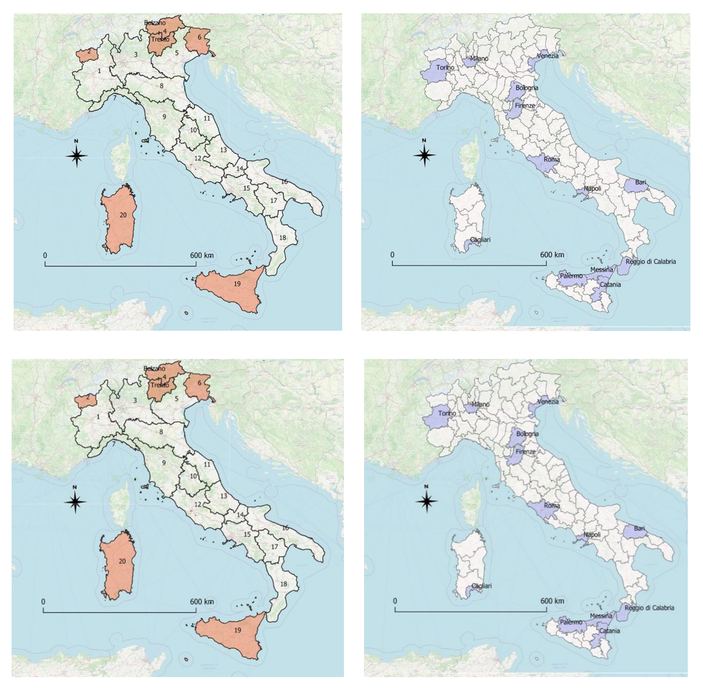
Figure 3.
Main characteristics of the Po Valley megalopolis in Italy: Authors elaborations from STAT data (2019); Turri, 2003.
Figure 3.
Main characteristics of the Po Valley megalopolis in Italy: Authors elaborations from STAT data (2019); Turri, 2003.

Figure 4.
Po Valley Megalopolis. (a) Regions, Population density (Population/km2); (b) railway lines and pollution map. Source: ISTAT (Regions); DeAgostini Base map (Geoportale Nazionale); ESA Nitrogen Pollution Map.
Figure 4.
Po Valley Megalopolis. (a) Regions, Population density (Population/km2); (b) railway lines and pollution map. Source: ISTAT (Regions); DeAgostini Base map (Geoportale Nazionale); ESA Nitrogen Pollution Map.

Figure 5.
Types of Spatial Diffusion Processes. Expansion, Relocation, Mixed. Authors elaboration from Haggett, 2001.
Figure 5.
Types of Spatial Diffusion Processes. Expansion, Relocation, Mixed. Authors elaboration from Haggett, 2001.

Figure 6.
Types of Spatial Diffusion Expansion Processes. Hierarchical/Waterfall. Authors elaboration from Haggett, 2001.
Figure 6.
Types of Spatial Diffusion Expansion Processes. Hierarchical/Waterfall. Authors elaboration from Haggett, 2001.
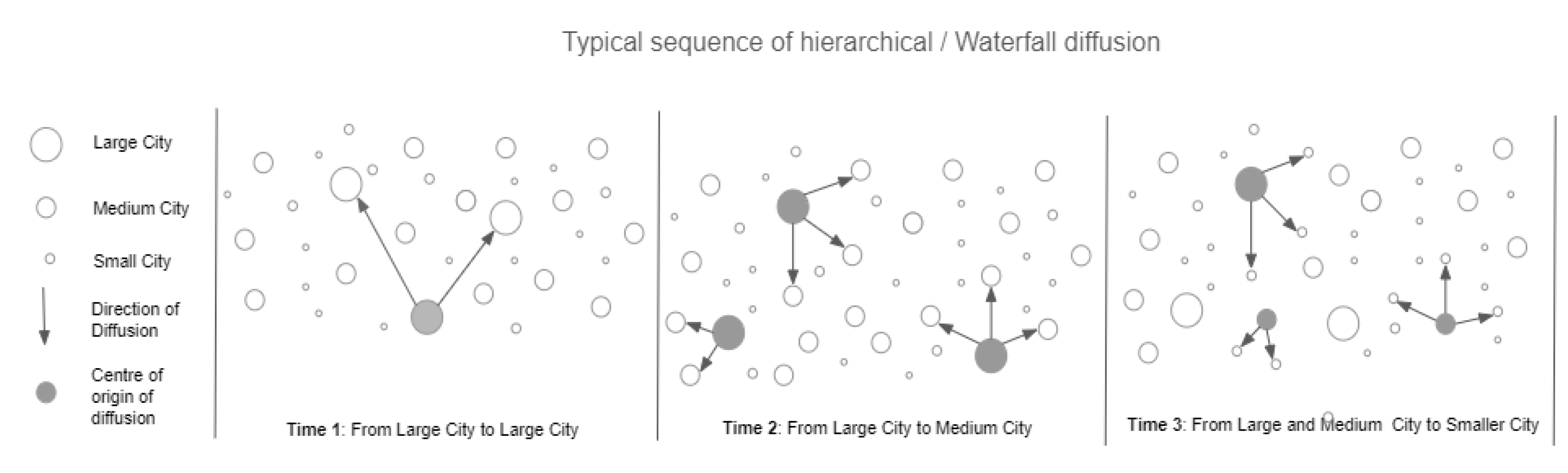
Figure 7.
Hierarchical Spatial Diffusion Process: Top-Down and Bottom-Up. Authors elaboration from Haggett, 2001.
Figure 7.
Hierarchical Spatial Diffusion Process: Top-Down and Bottom-Up. Authors elaboration from Haggett, 2001.

Figure 8.
Epidemic wave. Authors elaboration from Cliff AD, Haggett P. A swash-backwash model of the single epidemic wave. J Geogr Syst. 2006.
Figure 8.
Epidemic wave. Authors elaboration from Cliff AD, Haggett P. A swash-backwash model of the single epidemic wave. J Geogr Syst. 2006.

Figure 9.
Infographic data set. Source: Our elaboration on multiple sources (Appendix A).
Figure 9.
Infographic data set. Source: Our elaboration on multiple sources (Appendix A).

Figure 10.
COVID-19 related Deaths. (a). Deaths per 50,000 inhabitants; (b). Standardized Mortality Ratios. Source: our elaboration from data originally collected; ISTAT 2019 (population).
Figure 10.
COVID-19 related Deaths. (a). Deaths per 50,000 inhabitants; (b). Standardized Mortality Ratios. Source: our elaboration from data originally collected; ISTAT 2019 (population).
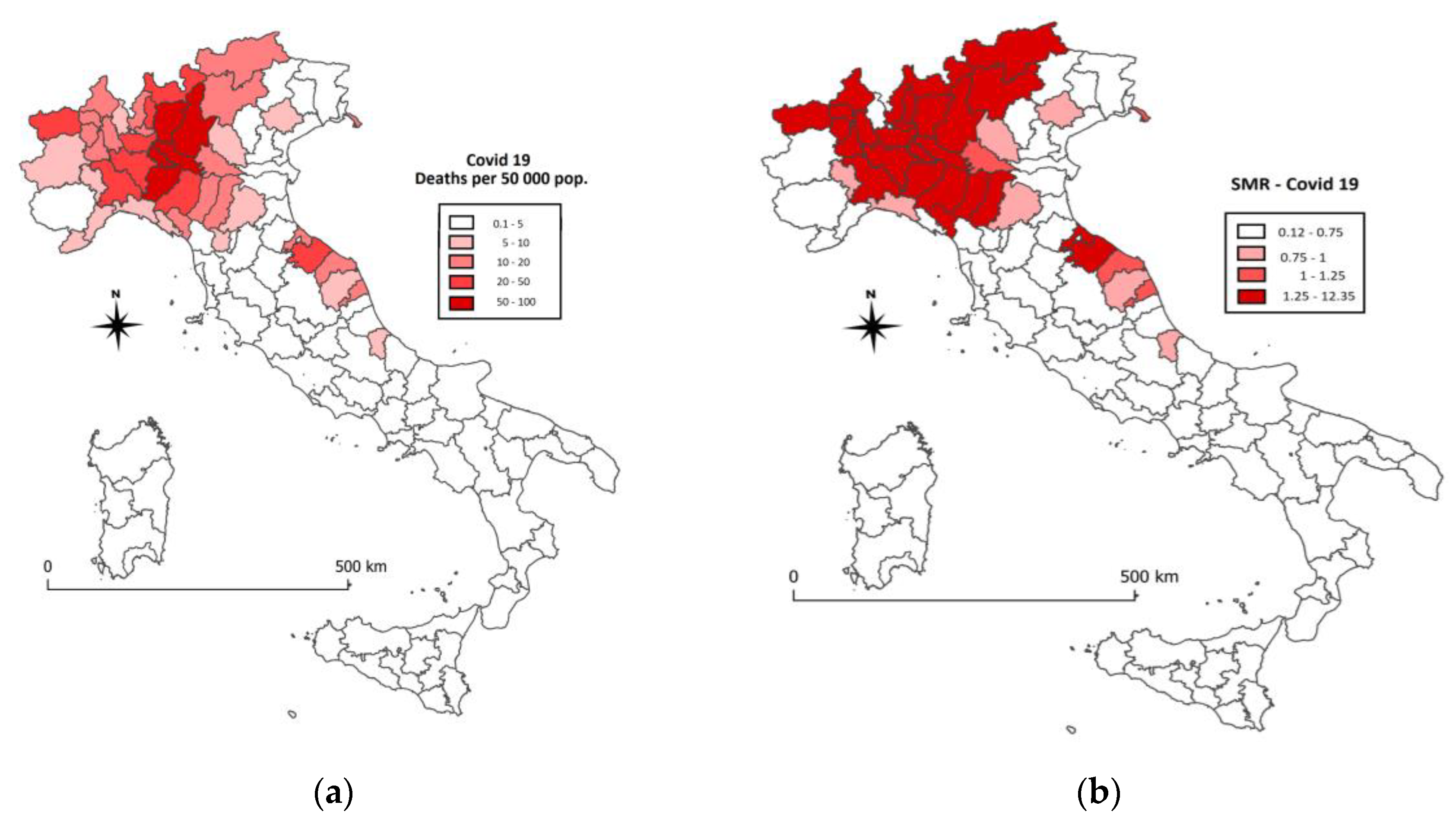
Figure 11.
Lisa Maps: Cov_57 Deaths; Cov_58 Contagions. Source: Our elaborations (GeoDa) from data as in Appendix A.
Figure 11.
Lisa Maps: Cov_57 Deaths; Cov_58 Contagions. Source: Our elaborations (GeoDa) from data as in Appendix A.

Figure 12.
Lisa Maps: Cov_65 Lethality; Cov_66 SMR. Source: Our elaborations (GeoDa) from data as in Appendix A.
Figure 12.
Lisa Maps: Cov_65 Lethality; Cov_66 SMR. Source: Our elaborations (GeoDa) from data as in Appendix A.
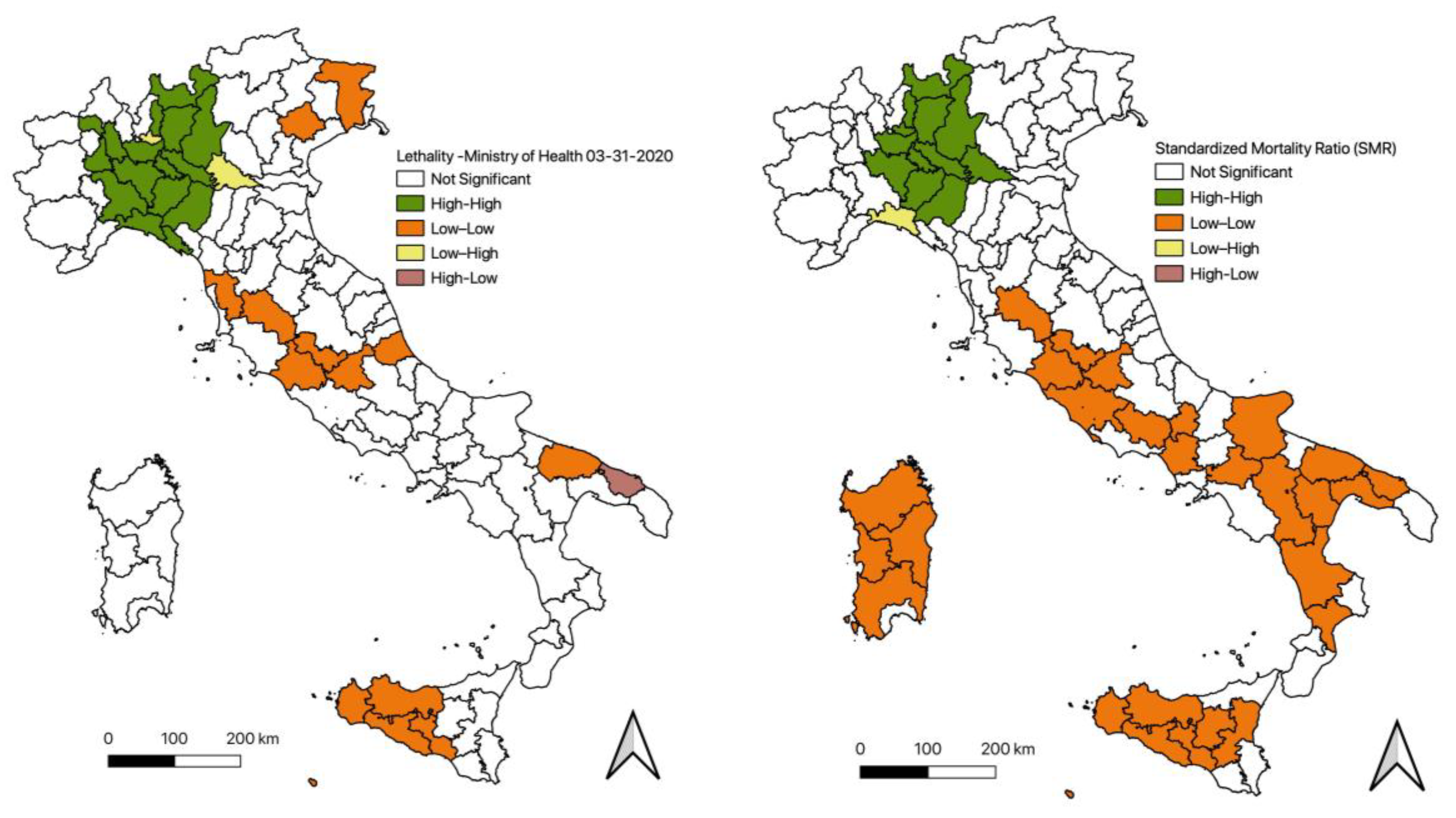
Figure 13.
Lisa Maps: (a) Cov_64 Inhabitants; (b) Cov_83 Commuting. Source: Our elaborations (GeoDa) from data as in Appendix A.
Figure 13.
Lisa Maps: (a) Cov_64 Inhabitants; (b) Cov_83 Commuting. Source: Our elaborations (GeoDa) from data as in Appendix A.

Figure 14.
Commuting indexes (a) Commuting index (1)—inflows-outflows/population; (b) Commuting index (2)—inflows plus outflows/internal flows.
Figure 14.
Commuting indexes (a) Commuting index (1)—inflows-outflows/population; (b) Commuting index (2)—inflows plus outflows/internal flows.
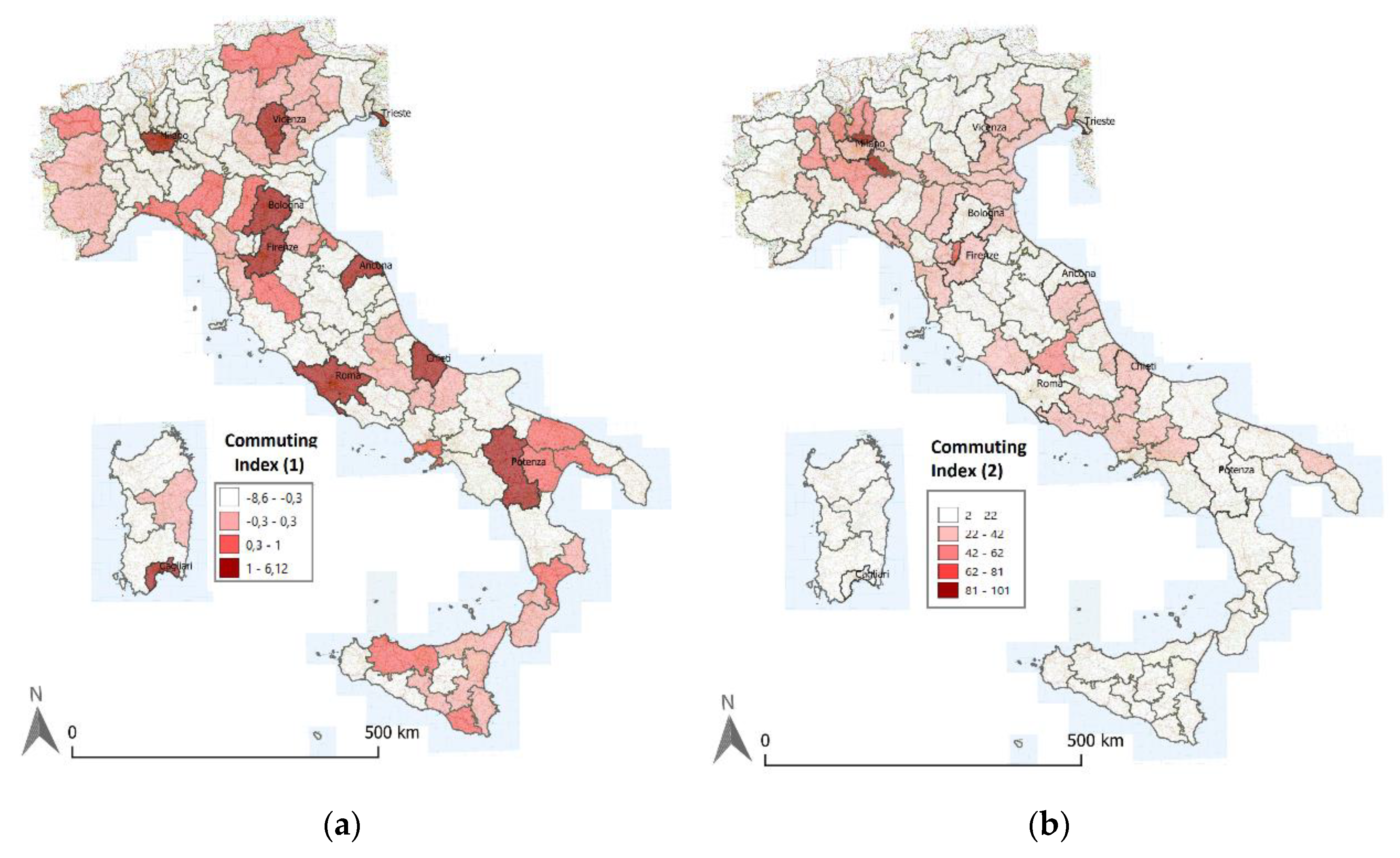
Figure 15.
Local Climate Change—Greater Milan Metropolis. Source: Authors elaboration from http://berkeleyearth.lbl.gov/city-list/.
Figure 15.
Local Climate Change—Greater Milan Metropolis. Source: Authors elaboration from http://berkeleyearth.lbl.gov/city-list/.

Figure 16.
WHO Regions which met the PM2.5 target in 2019. Source: Authors’ elaboration from https://www.iqair.com/.
Figure 16.
WHO Regions which met the PM2.5 target in 2019. Source: Authors’ elaboration from https://www.iqair.com/.
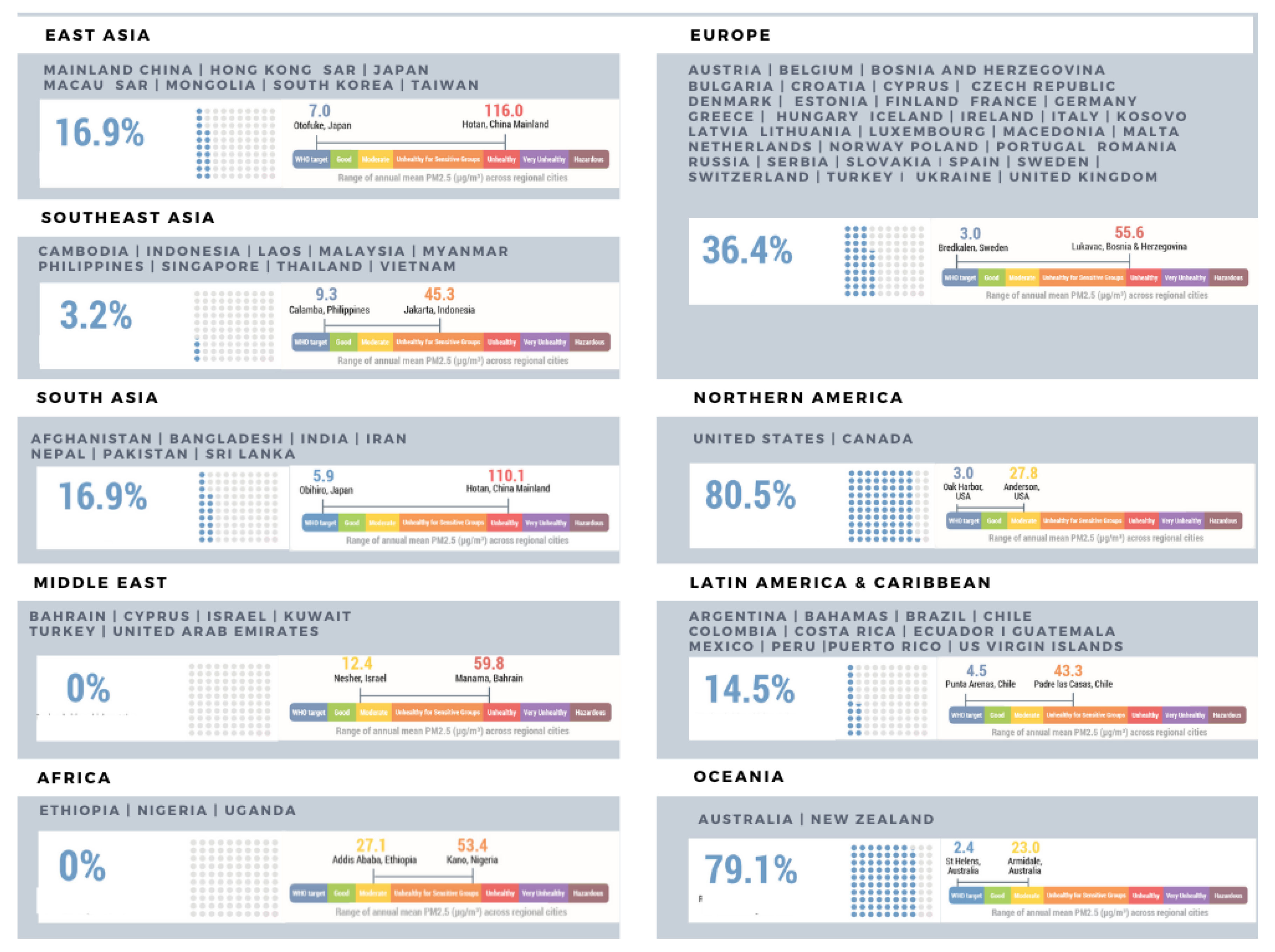
Figure 17.
Lisa Maps: Cov_14 PM2.5; Cov_15 PM10. Source: Our elaborations (GeoDa) from data as in Appendix A.
Figure 17.
Lisa Maps: Cov_14 PM2.5; Cov_15 PM10. Source: Our elaborations (GeoDa) from data as in Appendix A.
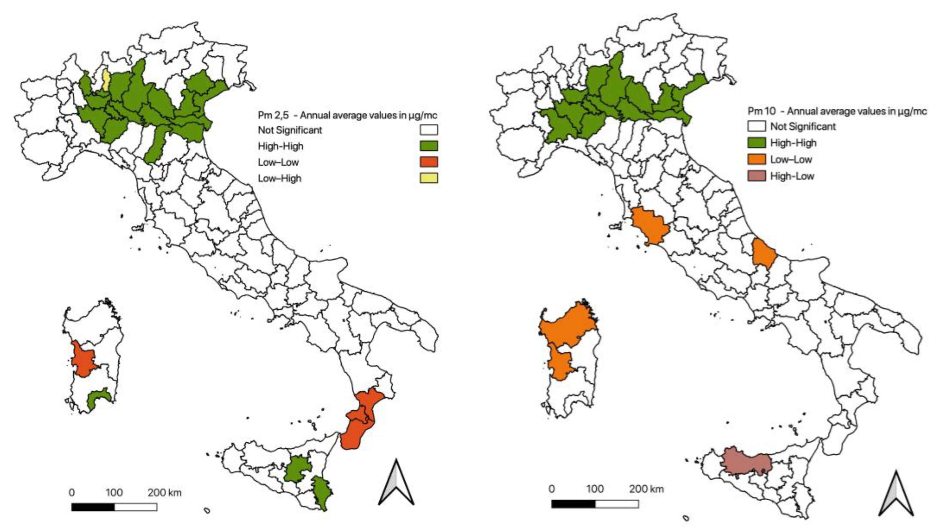
Figure 18.
Lisa Maps: Cov_19 Ozone (O3); Cov_72 PM10 and Ozone (O3). Source: Our elaborations (GeoDa) from data as in Appendix A.
Figure 18.
Lisa Maps: Cov_19 Ozone (O3); Cov_72 PM10 and Ozone (O3). Source: Our elaborations (GeoDa) from data as in Appendix A.
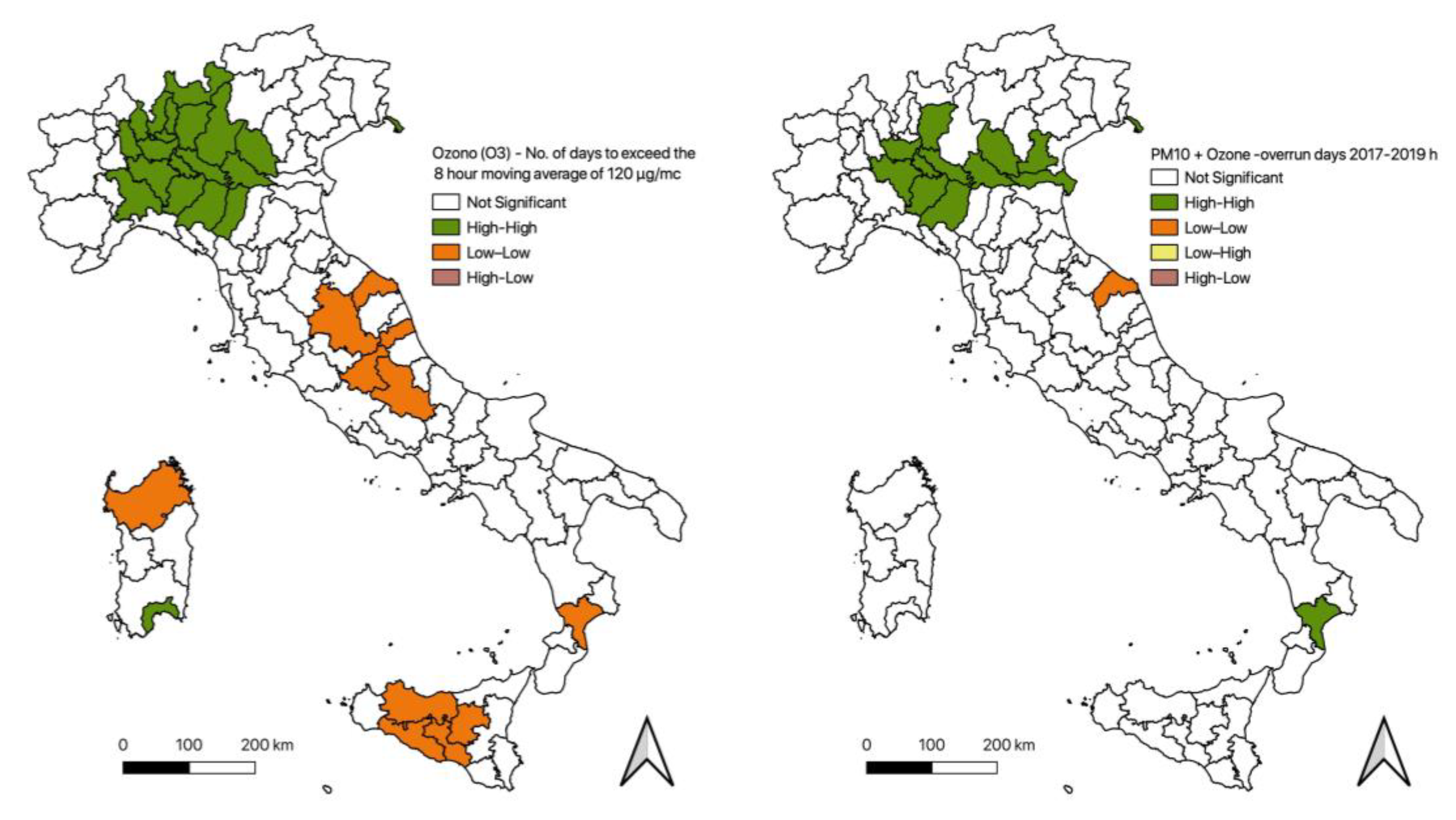
Figure 19.
Lisa Maps: Cov_37 Climate well-being index; Cov_39 Wind gusts. Source: Our elaborations (GeoDa) from data as in Appendix A.
Figure 19.
Lisa Maps: Cov_37 Climate well-being index; Cov_39 Wind gusts. Source: Our elaborations (GeoDa) from data as in Appendix A.
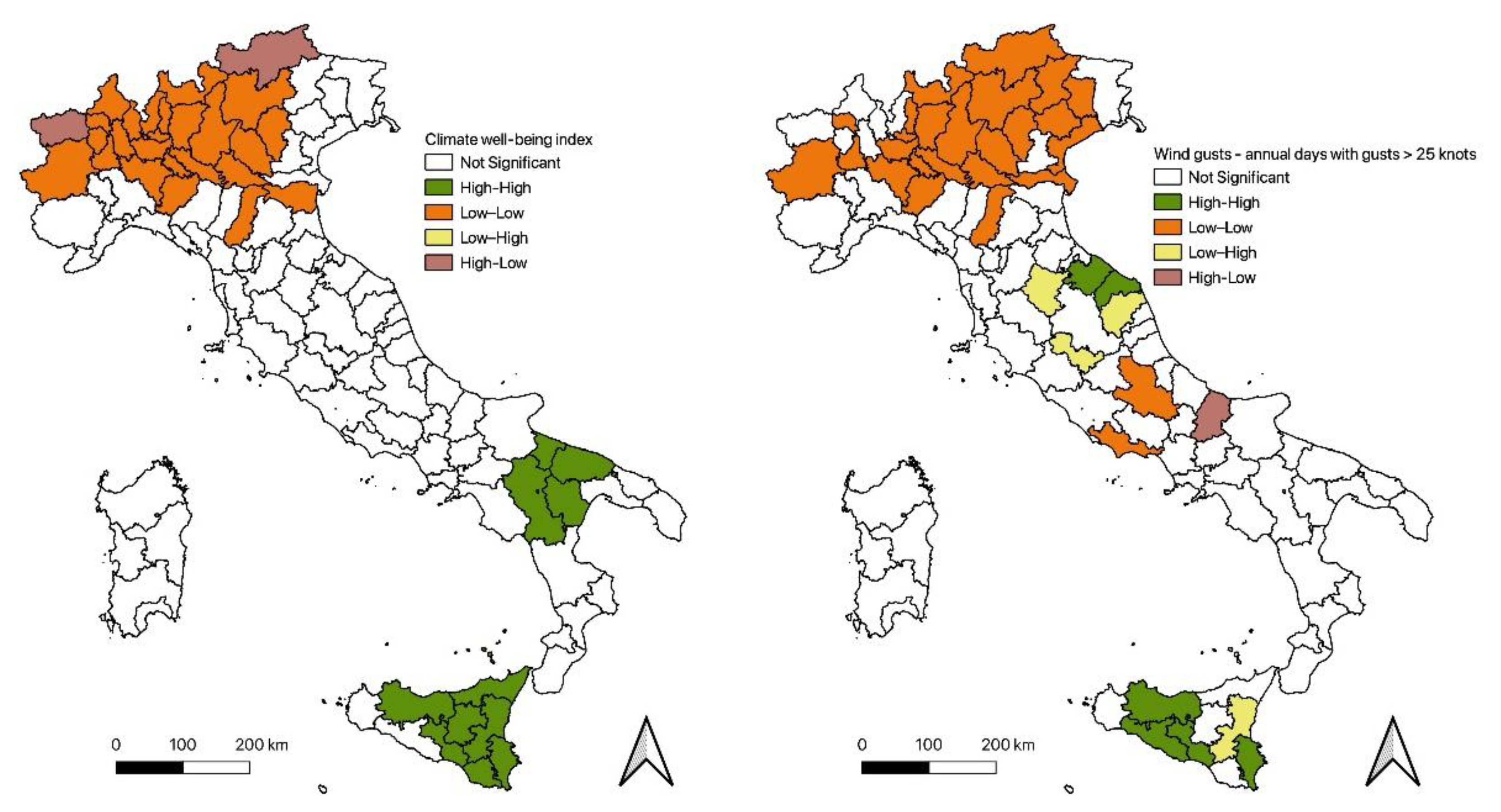
Figure 20.
Lisa Maps: Cov_41: Fog; Cov_55: wind Jan/Feb/Mar 2020. Source: Our elaborations (GeoDa) from data as in Appendix A.
Figure 20.
Lisa Maps: Cov_41: Fog; Cov_55: wind Jan/Feb/Mar 2020. Source: Our elaborations (GeoDa) from data as in Appendix A.
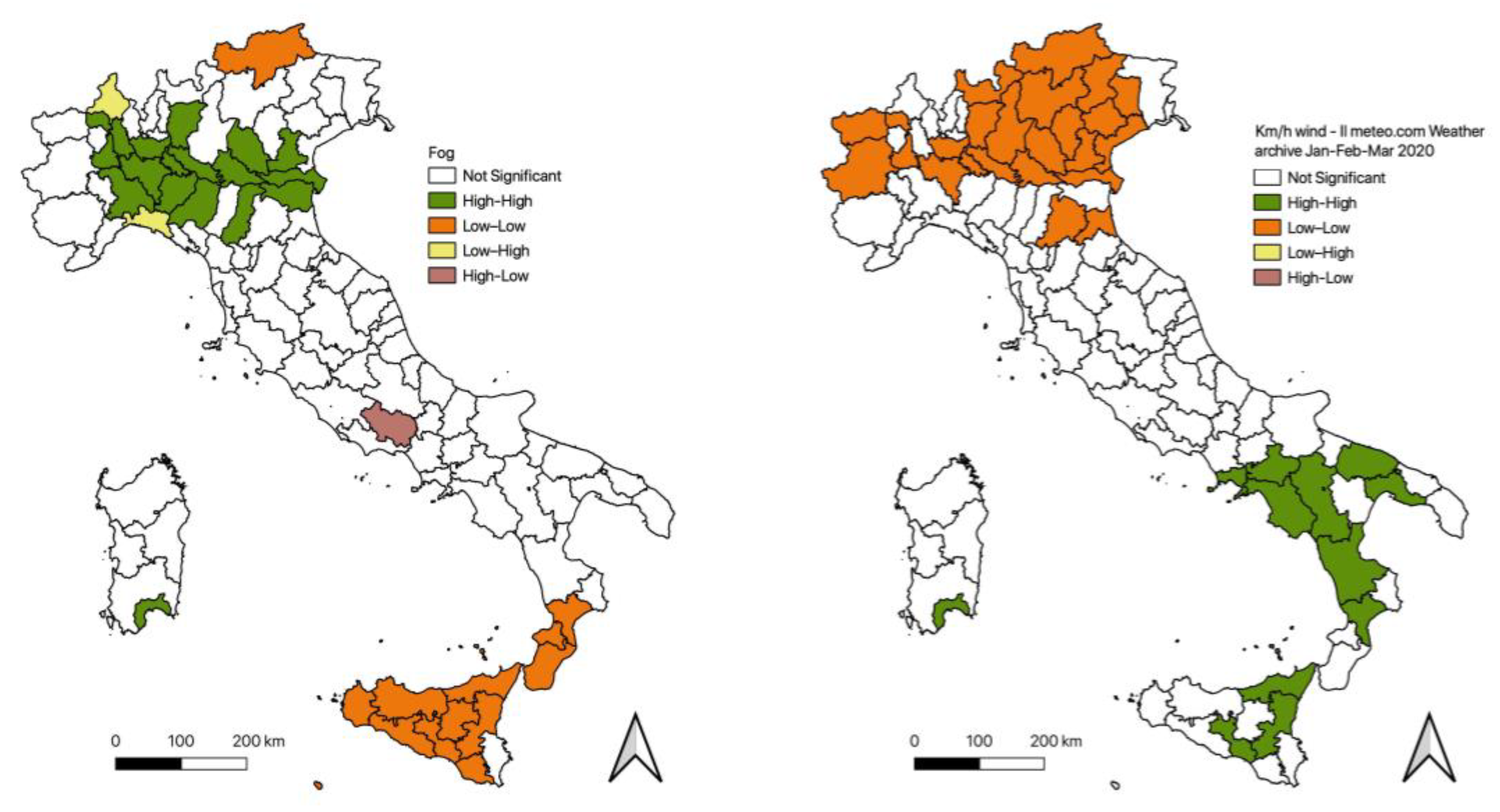
Figure 21.
Lisa Maps: Cov_49: sealed soils; Cov_82: CO2/non urbanized areas. Source: Our elaborations (GeoDa) from data as in Appendix A.
Figure 21.
Lisa Maps: Cov_49: sealed soils; Cov_82: CO2/non urbanized areas. Source: Our elaborations (GeoDa) from data as in Appendix A.

Figure 22.
Lisa Maps: Cov_3: land taken between 2014 and 2018; Cov_52: land take up to 2000. Source: Our elaborations (GeoDa) from data as in Appendix A.
Figure 22.
Lisa Maps: Cov_3: land taken between 2014 and 2018; Cov_52: land take up to 2000. Source: Our elaborations (GeoDa) from data as in Appendix A.
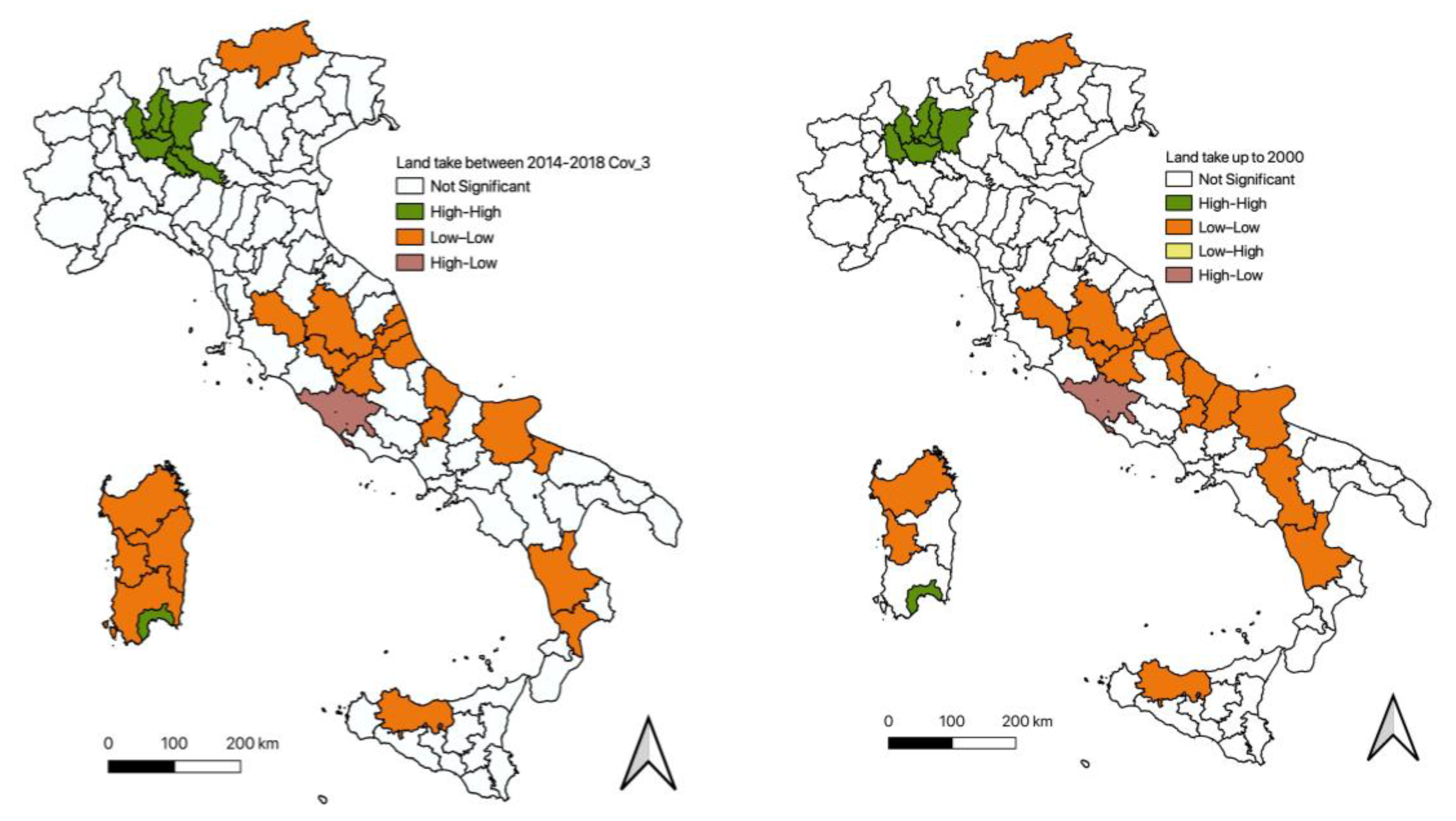
Figure 23.
(a) SMR; (b) Population density, motorways and average-sized provincial capital municipalities (100,000–200,000 population). Source: our elaboration from data originally collected; ISTAT 2019 (Population); Ministry of Transport and Infrastructure (Motorways).
Figure 23.
(a) SMR; (b) Population density, motorways and average-sized provincial capital municipalities (100,000–200,000 population). Source: our elaboration from data originally collected; ISTAT 2019 (Population); Ministry of Transport and Infrastructure (Motorways).
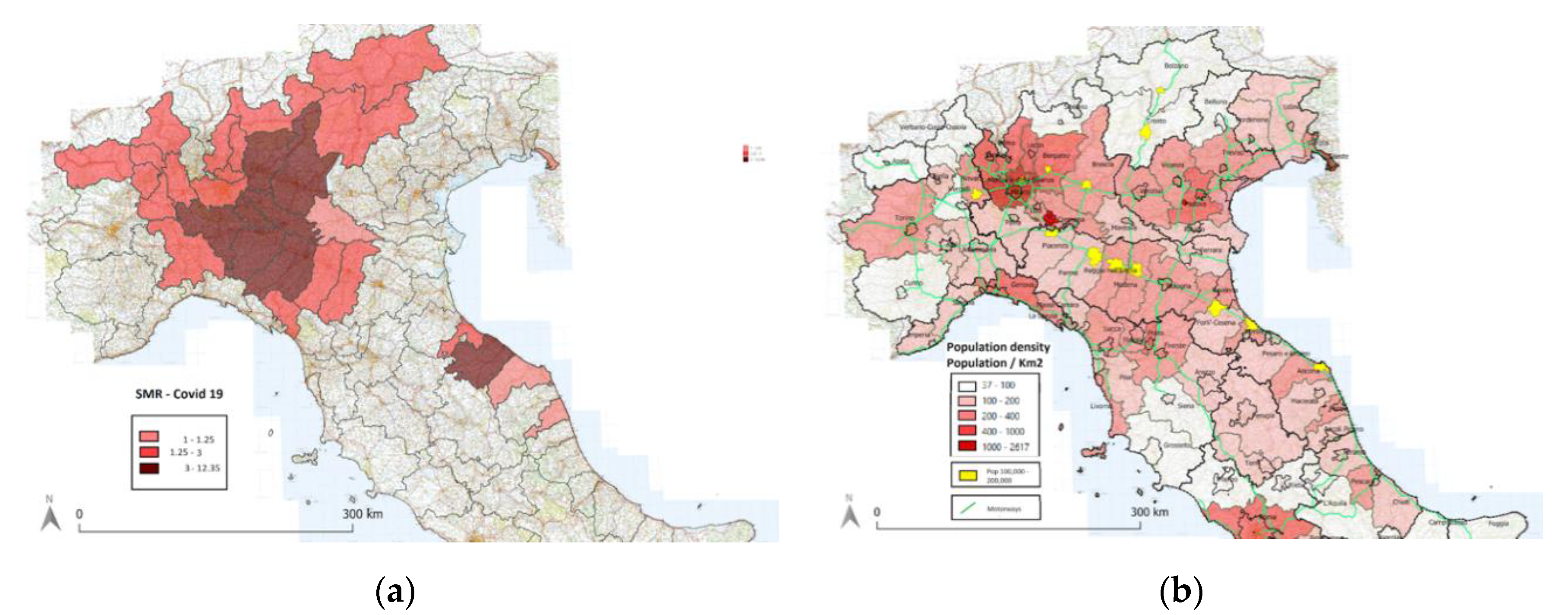
Figure 24.
PM10 equivalent—Po Valley Emilia Romagna. Source: our elaboration from La qualità dell’aria Emilia Romagna, 2018.
Figure 24.
PM10 equivalent—Po Valley Emilia Romagna. Source: our elaboration from La qualità dell’aria Emilia Romagna, 2018.

Figure 25.
Ecological approach and Policies—Po Valley Area. Our elaboration.

Figure 26.
Flattening curve of Earth’s carrying capacity based on comparing two possible scenarios: business-as-usual and sustainable.
Figure 26.
Flattening curve of Earth’s carrying capacity based on comparing two possible scenarios: business-as-usual and sustainable.

Table 1.
Selected Provinces ranked by SMR (>1).
| Province | Population (2019) | Population/km2 | Commuting Index (1) | Commuting Index (2) | SMR | PM10 + O3 * |
|---|---|---|---|---|---|---|
| Bergamo | 1114590 | 404.59 | −1.71 | 22.27 | 12.356 | 349 |
| Lodi | 230198 | 294.01 | −8.6 | 94.66 | 12.262 | 448 |
| Piacenza | 287152 | 111.05 | −0.62 | 23.67 | 10.013 | 299 |
| Cremona | 358955 | 202.75 | −3.94 | 41.76 | 9.583 | 417 |
| Brescia | 1265954 | 264.54 | −0.44 | 12.82 | 7.055 | 401 |
| Pavia | 545888 | 183.89 | −6.91 | 48.91 | 4.751 | 412 |
| Parma | 451631 | 131.01 | 0.79 | 14.62 | 4.494 | 342 |
| Pesaro | 358886 | 139.77 | −0.96 | 14.48 | 4.417 | 0 |
| Sondrio | 181095 | 56.67 | −0.3 | 8.82 | 2.763 | 35 |
| Aosta | 125666 | 38.54 | 0.86 | 6.51 | 2.723 | 61 |
| Milano | 3250315 | 2063.05 | 6.12 | 38.17 | 2.699 | 405 |
| Lecco | 337380 | 418.79 | −3.08 | 56.45 | 2.572 | 282 |
| Reggio Emilia | 531891 | 232.15 | −1.11 | 27.85 | 2.493 | 364 |
| Alessandria | 421284 | 118.38 | −0.48 | 20.36 | 1.974 | 417 |
| Trento | 541098 | 87.18 | −0.18 | 4.62 | 1.892 | 84 |
| Biella | 175585 | 192.26 | −0.57 | 21.04 | 1.857 | 184 |
| Novara | 369018 | 275.34 | −2.13 | 36.33 | 1.686 | 155 |
| Rimini | 339017 | 391.92 | 0.81 | 21.16 | 1.647 | 263 |
| Verbania | 158349 | 70.04 | −0.88 | 13.85 | 1.560 | 45 |
| Como | 599204 | 468.49 | −2.64 | 45.88 | 1.558 | 225 |
| Modena | 705393 | 262.43 | 0.71 | 22.69 | 1.529 | 383 |
| Bolzano | 531178 | 71.8 | 0.4 | 2.31 | 1.441 | 26 |
| Vercelli | 170911 | 82.11 | −1.31 | 52.77 | 1.339 | 82 |
| Massa | 194878 | 168.78 | −2.76 | 37.26 | 1.293 | |
| Monza | 873935 | 2155.69 | −5.98 | 101.24 | 1.255 | 413 |
| Mantova | 412292 | 176.09 | −1.43 | 29.31 | 1.225 | 343 |
| Trieste | 234493 | 1103.48 | 1.34 | 11.96 | 1.211 | 32 |
| Fermo | 173800 | 201.45 | −1.05 | 27.93 | 1.143 | |
| Ancona | 471228 | 240.03 | 1.31 | 15.07 | 1.086 |
Source: our elaboration from multiple datasets. See Appendix A for details. * Days over law limits of PM10 + O3 (2017–2019); (1) Commuting index (inflows-outflows/population); (2) Commuting index (inflows + outflows/internal flows).
© 2020 by the authors. Licensee MDPI, Basel, Switzerland. This article is an open access article distributed under the terms and conditions of the Creative Commons Attribution (CC BY) license (http://creativecommons.org/licenses/by/4.0/).
Share and Cite
MDPI and ACS Style
Murgante, B.; Borruso, G.; Balletto, G.; Castiglia, P.; Dettori, M. Why Italy First? Health, Geographical and Planning Aspects of the COVID-19 Outbreak. Sustainability 2020, 12, 5064. https://doi.org/10.3390/su12125064
AMA Style
Murgante B, Borruso G, Balletto G, Castiglia P, Dettori M. Why Italy First? Health, Geographical and Planning Aspects of the COVID-19 Outbreak. Sustainability. 2020; 12(12):5064. https://doi.org/10.3390/su12125064
Chicago/Turabian StyleMurgante, Beniamino, Giuseppe Borruso, Ginevra Balletto, Paolo Castiglia, and Marco Dettori. 2020. "Why Italy First? Health, Geographical and Planning Aspects of the COVID-19 Outbreak" Sustainability 12, no. 12: 5064. https://doi.org/10.3390/su12125064
Note that from the first issue of 2016, this journal uses article numbers instead of page numbers. See further details here.