Real Estate Investment Choices and Decision Support Systems
by
 , ,
, ,
Vincenzo Del Giudice
1, 
Pierfrancesco De Paola
1,*,
Torrieri Francesca
1,
Peter J. Nijkamp
2,3 and
Aviad Shapira
4 1
Department of Industrial Engineering, University of Naples “Federico II”, Piazzale V. Tecchio, 80125 Naples, Italy
2
Jheronimus Academy of Data Science, ‘s-Hertogenbosh 5200–5249, The Netherlands
3
Department of Spatial Economics, Vrije Universiteit Amsterdam, De Boelelaan 1105, 1081 HV Amsterdam, The Netherlands
4
Technion—Israel Institute of Technology, Faculty of Civil and Environmental Engineering, 3200003 Haifa, Israel
*
Author to whom correspondence should be addressed.
Sustainability 2019, 11(11), 3110; https://doi.org/10.3390/su11113110
Submission received: 4 March 2019
/
Revised: 23 May 2019
/
Accepted: 27 May 2019
/
Published: 2 June 2019
(This article belongs to the Special Issue Real Estate Landscapes: Appraisal, Accounting and Assessment)
Abstract
:The evaluation of real estate assets is currently one of the main focal points addressed by territorial marketing strategies, with the view of developing high-performing or competitive cities. Given the complexity of the driving forces that determine the behavior of actors in a real estate market, it is necessary to identify a priori the factors that determine the competitive capacity of a city, to attract investments. The decision support system allows taking into account the key factors that determine the “attractiveness” of real estate investments in competitive urban contexts. This study proposes an integrated complex evaluation model that is able to map out and encapsulate the multidimensional spectrum of factors that shape the attractiveness of alternative real estate options. The conceptual–methodological approach is illustrated by an application of the model to a real-world case study of investment choice in the residential sector of Naples.
1. Introduction
This study presents a new research design aimed at assessing how investment decisions of different agents operating in the residential real estate market are affected by a multidimensional choice of factors, including environmental and social attributes that might vary across different territorial contexts. In general, residential location choice behavior has been widely addressed in the academic literature, with particular reference to the impact of the transportation system and location attributes of an area on the decision context [1,2,3,4,5,6,7,8,9,10,11,12,13,14,15,16,17,18,19,20,21,22,23].
In general, studies on residential location traditionally fall into two main groups: (i) The market approach, associated with researchers such as Alonso [23]; and (ii) the nonmarket approach, associated with sociologists such as Rex and Moore [24]. It is noteworthy that, in terms of the explanation of broader social science phenomena such as housing dispersion, gentrification, and abandonment, Hoang and Waley [25] have highlighted the importance of the nonmarket approach; they argue that housing status and dwelling quality appear to be more important determinants of the existing patterns of residential location than access–space trade-off. However, despite the solid theoretical underpinnings of their work, it might be viewed as supplementing rather than replacing the market approach, given that in most empirical work, housing status has been defined partly in terms of distance from the city center and access to the street [26].
Many researchers have developed a different residential location choice model in order to analyze the demand of households for housing, transportation, and the living environment [27]. According to the economic theory, household residential choices are functions of different housing and location attributes that are differentiated by a variety of household characteristic [28].
These attributes have a relative importance and influence the choice behavior of the households. Among the various factors that influence residential location choices, transportation accessibility has long been recognized as one of the most important factors and also has a great impact on the attributes that characterize property type, traffic noise, air quality, municipal taxes or rent, and services [29]. In the international literature, it has also been recognized that the real estate market is location-specific and highly fragmented, and so the importance of the relevant attribute can be modified depending on the context [30].
In this paper, we present an integrated real estate choice model, mainly oriented towards those qualitative attributes—relative to the dwelling and territorial context—that influence this choice. In particular, the present study aimed at developing an integrated complex evaluation model, reflecting the multidimensional spectrum of factors affecting the attractiveness of alternative residential real estate property and location, based on the integration of a multicriteria evaluation model and the stated preferences (SP) experiment in order to evaluate the impact of different attributes on residential choice location in the specific context of Naples.
Starting with a literature review, a comprehensive list of attributes that characterize diverse property types and locations was defined; then, on the basis of the Analytic Hierarchy Process (AHP), the most important attributes were selected by considering the point of view of a sample of different agents.
In our study, a first experiment was carried out, to test the proposed methodology and to envisage an appropriated questionnaire, to identify which of the attributes that characterize each location predominantly influences the behavior of different agents.
The proposed model considers that choices in the residential real estate market are characterized by many uncertain factors, determined by the nontypical conditions and a high complexity of the market in question [31], both from the demand and the supply side. In this context, we developed a measurable “attractiveness” function for each territory. The metropolitan area of Naples was used next as a first case study to test our analysis framework.
This paper is organized as follows: In Section 2, we present an overview of the issues concerning residential location choice behavior, with particular reference to the methodological approach adopted by us. Next, after an introduction, in Section 3.2 and Section 3.3, we present the results of a survey designed to select the relevant attributes to be included in the model, assessed on the basis of a questionnaire structured according to the analytic hierarchy process [32,33]. In Section 3.4, a stated preference (SP) survey is presented for the assessment of different alternative investment choice locations characterized by various attributes. The applied choice experiment was structured in accordance with the guidelines of the “Catalogue of Computer Programs for the Design and Analysis of Orthogonal Symmetric and Asymmetric Fractional Factorial Experiments” [34]. Conclusions and further research perspectives follow in Section 4.
2. Residential Location Choice Model: Issues and Approaches
Numerous studies in the international literature have developed residential location choice models [34]. Alonso [23] explained personal residential choice behavior on the basis of the concept of utility maximization. He argued that household utility can be measured by the expenditure in goods, the distance from the main urban infrastructures, and the size of the land lots. Later, Muth [35], Mills [36], Evans [37], and Wheaton [38] extended the model, which is referred to as the classical urban land market model. McFadden developed another school of thought on modeling residential location choices, based on the discrete choice framework [39]. One of the most important advantages of this approach is that it enables researchers to consider the physical and social characteristics of the surrounding environments, as well as housing attributes, based on the random utility maximization theory. Through this, researchers can understand how household trade-off among various choice sets can influence the choice of residential location. Moreover, this approach provides a way of understanding how the interaction between sociodemographic attributes and spatial characteristics affects household residential choices through interaction terms [40,41].
In reality, the household residential location choice is a complex function of a wide-range of housing and location attributes. It is well-known that the value of a property depends on its intrinsic and extrinsic characteristics, and that the relative importance of these attributes vary across different types of households and contexts. In reality, consumers differ substantially in their tastes for housing and might also display bounded rationality, with the consequence that a great variety of responses might result from the presentation of the same well-defined alternatives to each consumer in a population. Further, the housing market might be slow in adjusting to the equilibrium, making arbitrage a profitable activity. Clearly, due insight into consumer tastes, responses, and behavior in the area of housing location decisions—or, more generally, real estate decisions—is needed [39].
The present paper presents a decision support system that is able to include these elements of uncertainty and heterogeneity. In particular, the decision support system originates from the housing location choice theory proposed by McFadden in the 1990s [42], assuming an extension of the neoclassical economic model to simulate consumer choice behavior. Assuming the classical model of a rational utility maximizing consumer, it is assumed that the utility function itself is not known in advance by the analyst [39]. Based on this assumption, the perceived utility Uij can be expressed as the sum of two specific components: An ordinal utility component and a random residual. The ordinal utility is the average of the expected value of the perceived utility among all users with the same choice context of decision i. The random residue εij is the deviation from the perceived utility compared with the expected value for all effects of the various determinants that introduce uncertainty in the modeling choice. Indeed, in the real estate market, there are substantial differences between the actors involved in a decision-making process, depending on the purposes of investment (final use, investment, safety, etc.), on the object of the investment, and on the strategic of the operator.
When focusing our attention on the residential location choice problem, the variables of the choice model refer, on the one hand, to the specific class of actors (and thus, to the attributes characterizing them), and on the other, to the definition of a utility function for each investment destination. Thus, in this specific case, the rational subject is represented by users–owners and tenants and the alternatives of choice are represented by the geographical space (territory) in which the economic subject chooses to make the investment.
The areal utility function—or perceived attractiveness—is the capacity of a territory to attract investments in a specific relevant submarket. Indeed, according to the hypothesis of rational decision making, an investor will choose the alternative (territory, or locality) which maximizes their utility function. Then the likelihood of choosing one territory over the others will be determined by a number of attributes or characteristics of the territory itself, so that the investor can achieve their objectives. Given the complexity that characterizes individual territorial reality, the utility function will be a composed function, in which several attributes contribute to its definition, i.e., attributes relating to the economic, environmental, social, and institutional context, and to physical characteristics. In general, we assume, for the specific case under construction, a linear attractiveness function, without ignoring, though, the possibility of using other specific functional forms of aggregation of the various attributes [43].
In the next section, we present the methodology deployed to define an integrated model for the simulation of choice behavior in the real estate market. In particular, we propose a novel integration of the analytic hierarchy process with a stated preference approach in order to evaluate and select the relevant attributes that enter the utility function.
3. The Proposed Methodology
The present section presents an integrated methodology for defining a random utility model for real estate investments in relation to residential location choice. In particular, this paper focuses on the definition of attributes relevant for the calibration of the real estate choice model.
We offer here an integrated methodological approach where the use of two different methodologies contributes to the design of a decision support system (DSS) for residential location choice. This DSS has a dual objective: To support, on the one hand, the economic subject looking for where to invest, and, on the other, decision makers in a given territorial market activity, highlighting the factors that determine the attractiveness of a place. Based on the general assumptions of a discrete choice model, the proposed study was logically organized in four sequential steps (see Figure 1), each of which is characterized by different objectives, instruments, and moments of analysis:
- ▪
- A first step where a general list of attributes is identified on the basis of studies conducted in the international context;
- ▪
- A second step where an assessment of relevant attributes is considered for the specific area examined (Municipality of Naples) by means of the analytic hierarchy process;
- ▪
- A third step where a stated preference experiment is carried out to evaluate different alternatives characterized by the relevant attributes assessed in the previous phase. The questionnaire was structured here using a fractional factorial design;
- ▪
- A fourth and final step that consists of the calibration of the coefficients of the choice model by the use of a multinomial logit model.
These steps of our methodology are described in greater detail in Section 3.1, Section 3.2, Section 3.3 and Section 3.4.
3.1. Step 1: The Selection of Attributes
The selection of the attribute to define the utility or attractiveness function was carried out based on a literature review of the case studies developed in the last year in the international literature. The literature review was done using the Scopus database and considering as our key words “Residential location choice model” and “Discrete choice model”, and “Real estate market” looking at papers published in open access journals.
In this review, we considered residential location choice studies employing the discrete choice framework. Within this framework, a decision maker chooses a single alternative from a set of mutually exclusive alternatives, the choice set, thus obtaining a certain level of utility from each alternative and choosing the alternative providing the most utility. A residential location choice, by definition, is a spatial choice and, as such, description of the residential alternative consists partly of residential unit and alternative location attributes. As argued by Susilo et al. [44], the understanding of people’s preferences should not be framed solely through physical characteristics, but the inclusion of social aspects will add significance effects on people’s decisions.
Actually, the results obtained showed that numerous studies have been carried out in the international literature on residential choice models [27,45,46,47,48,49,50,51,52,53,54,55,56], and a wide variety of explanatory variables have been considered in relation to property type, location, and social attributes. In Table 1, a synthesis of the study analyzed is reported.
Starting from the abovementioned study, a general list of attributes is presented, taking into account the specific context under investigation. In the definition of each attribute, much attention was given to the ‘perception’ that decision makers have of the quality of places.
A detailed description of the attributes is reported in Table 2. In the next section, the methodology to assess the relevant attributes for the specific context is presented.
3.2. Step 2: The Assessment of Relevant Attributes
The methodology proposed for the evaluation of relevant attributes was based on the analytic hierarchy process developed by Saaty in the 1970s [32,33]. Starting from a general list of attributes (see Table 2), a questionnaire was presented to a select number of experts from the Departments of the Faculty of Engineering at the University of Naples “Federico II”, in order to identify those elements that most likely influence the housing choice in the context of the Naples Metropolitan area. The questionnaire, according to the AHP logic, requires respondents to express a nominal preference for the attributes selected through pairwise comparisons. The results obtained from each individual questionnaire represent the weights and therefore the importance associated to each attribute. These weights were then aggregated by means of the aggregating of individual priorities (AIP) technique in order to obtain the total weights of attributes.
In a decision-making process, there are various ways to aggregate information in the presence of many decision makers. In the literature, two ways are advocated in particular [57], namely:
- ▪
- Aggregation of individual judgments (AIJ): Consisting of aggregating individual judgments for each set of pairwise comparisons, in an aggregate hierarchy;
- ▪
- Aggregating of individual priorities (AIP): Consisting of synthesizing each individual hierarchy and the resulting aggregate priorities, in order to reach the rational choice of the group from individual choices.
In this study, we chose to proceed by following the second mode (AIP), as the concept of a “group” in the AIP mode is more in agreement with our case study: The AIJ considers the group of decision makers as a single entity, while the AIP sees it as a set of separate individuals. In the first case, the group behaves as if it were a single individual: Individual identities are lost at every stage of aggregation, and the result expresses the priorities of the group. In the second case, however, it is assumed that the various decision makers have different influences on the final choice, and therefore, it is important to take into account a different system of values. This approach seems more appropriate for the case being considered. The aggregation function used is the geometric mean that meets the conditions underlying the method [32]:
where wi are the eigenvectors and aij indicates how much more (or less) important the i-th element is than the j-th element.
The proposed questionnaire was compiled on the basis of expert opinion and with reference to guidelines prepared by the NOAA panel (National Oceanic and Atmospheric Administration), in order to obtain an effective and appropriate tool for measuring the necessary information to be collected. This was because the questionnaire is a communication tool and, as such, its main objective is to transfer the information to the respondent as clearly as possible. On the other hand, the questionnaire also represents a measuring instrument, whose function is to collect and digest data and information on the attributes under investigation. The questionnaires collected were divided into three groups based on the age and the social and economic characteristics of the respondents.
The first group in our sample of interviewees (GR1) included 17 interviewees, those aged 20 to 35 and mainly tenants or residents in the family home; the second group (GR2) included 9 interviewees, those aged 35 to 50, who were owners or tenants; and the third group (GR3) included 12 interviewees, those aged 50 to 65, who were again owners or tenants. Table 3 shows the estimated weights as ordinal rankings for each group.
The weight assessed for each of the three rankings was next aggregated through the AIP methodology in order to define the aggregate set of weights. The results are shown in Table 4.
The results reported in Table 4 show that the contextual characteristics have the greatest importance in the residential location choice, confirming also the assumptions underlying the study. Looking at the attributes, we can make the following observations:
- As regards the building characteristics, the variables that have the greatest influence on real estate choice are the intrinsic positional aspects, the presence of parking, and the dwelling size. This result is strongly confirmed by the dynamics of the local real estate market. In fact, considering the market value as a budget constraint, the most significant variables are likely to reflect the main characteristics and problems of the metropolitan area of Naples. The particularities of the urban landscapes favor the choice of buildings characterized by panoramic views or positive environmental characteristics, just as the problem of traffic and parking spaces favors buildings where there is opportunity for parking;
- As regards the characteristics of the urban spatial context, the attributes related to environmental issues and the socioeconomic context have a preponderant weight, and this result is a factor also reflected in the local market.
On the basis of the results obtained, we chose to focus our analysis and definition of the SP survey only on the contextual variables, in order to understand how environmental quality, the socioeconomic context, and accessibility do influence the residence location choice.
The need to focus our attention on a relatively small number of attributes comes from the experimental SP design. In fact, there is evidence that an economic actor does not choose an alternative good itself but considers the attributes that characterize it, and thus, the change in the levels of attributes (as is witnessed in multi-attribute utility theory [58]). Therefore, the greater the number of attributes on which the choice is based, the more difficult it is for the decision maker to make a conscious comparison with the alternative proposed.
The next section concerns now the description and implementation of the SP experiment for the assessment of different choice location options is characterized by different attributes.
3.3. Step 3: Stated Preference (SP) Experimental Design
The implementation phase of an SP survey is one of the most sensitive stages of the analysis, because its objective is to induce those interviewed to express their preferences with respect to a set of alternative scenarios. In general, surveys used to gather basic information are of two different categories: Surveys of actual behavior in a real context (revealed preference or RP surveys) or surveys of hypothetical behavior in fictitious scenarios (stated preference or SP surveys). The traditional method of revealed preference is based on surveys. This method provides information on users’ actual choices in situations relevant for the model to be calibrated. Survey design therefore consists of the definition of the sample size, the questionnaire, and the sampling strategy. SP surveys, on the other hand, are conceptually equivalent to a laboratory experiment designed with a larger number of degrees of freedom. SP refers to a set of techniques that use statements made by interviewees about their preferences in hypothetical scenarios and are based on the possibility of “controlling the experiment” by designing the choice context rather than recording choices in a given (generally uncontrolled) choice context, which was the case with RP surveys.
SP surveys have several advantages over RP surveys, which can be summarized as follows:
- ▪
- They allow the investigation of choice alternatives not available at the time of the survey (e.g., new modes or services in a mode choice context);
- ▪
- They can control the variation of relevant attributes outside the presently observed range to obtain better estimates of the corresponding coefficients; for example, the monetary cost of travel in urban areas usually falls within a limited range of values;
- ▪
- They can introduce new attributes not present in the real choice context;
- ▪
- They can collect more information, i.e., larger samples, per unit cost, since each interviewee is usually asked about several choice contexts.
These advantages are obtained at the price of introducing some distortion in the results and in the models. Distortions stem from the possible differences between stated and actual choice behavior: If the user experienced a real situation, his/her behavior might be different from that stated during the SP survey. These differences in behavior may be due to a variety of factors. For example, the context suggested might be or appear to be unrealistic, some attributes of the suggested alternative relevant to the decision maker might be missing, or there may be fatigue and justification bias effects. However, it should be noted that some of these problems are inherent to the SP survey technique, while others can be solved by careful design and execution of the surveys, bringing them as close as possible to real choice contexts.
In the light of the above, it is clear that SP surveys, in spite of their considerable application potential, should be seen as complementary to, rather than competing with, RP techniques. The advantages and disadvantages of the two techniques compensate for each other and, as will be seen, the techniques can be used jointly to build the integrated models.
In a first step of the analysis, we considered referring to an SP approach to assess the complex values (use value, non-use value) rather than just use values of dwelling.
In an SP experiment, the respondents are offered hypothetical alternatives in order to evaluate and to express their preference for the alternatives in various ways. The SP approach has a number of advantages compared to RP methods. It can avoid correlation problems, ensure sufficient variation in data, offer a better trade-off between variables than often exists in the real world, help to collect multiple choices per person, and avoid measurement errors in the independent variable. Each alternative presented to the respondents is characterized by a set of relevant attributes. The levels or values associated with each attribute must be realistic and are usually combined according to the rules of an experimental design procedure so as to permit trade-offs between attributes [46,50,51,52,59].
An SP experiment consists of a number of elements: The composition of the choice contexts proposed to the decision maker/interviewee, the selection of the choice context proposed, the type of preference response elicited from the decision maker, and the way in which the interview is conducted [60].
There is a logical sequence of tasks required to design an SP choice experiment, as indicated by Louviere et al. [59], Hensher [61], and Pearmain et al. [62]. Firstly, we must identify and select the attributes to be included in the choice experiment. Walker et al. [50] suggest not considering more than five attributes in each scenario, in order to make the choice as clear as possible for the interviewee. Secondly, it is necessary to identify for each attribute a unit of measurement that is not always uniquely determined. After establishing the scales for measuring the attributes, we must then define the levels of each attribute and finally proceed to build and structure the choice experiment.
The choice experiment can be appropriately structured using a full factorial design, which considers all possible combinations of attributes and their levels. In most cases, the number of theoretically possible scenarios is very high, because splitting n factors, k groups (i = 1, 2, …, k), and ni elements taking m levels, the total number of scenarios will be:
There are various techniques to reduce the number of scenarios generated by a full factorial design; one of these is a fractional factorial design, which allows just a subset of the scenarios to be used, permitting orthogonal estimation, which is usually constructed to eliminate main-effect correlation between attributes. By following the logical sequence mentioned above, an SP experiment was defined by deploying the attributes selected in the previous step. For each of them, a measurement unit and its corresponding levels were identified (see Table 5).
More specifically, accessibility is measured in terms of total time taken for a single trip (in minutes, using the intervals: +5 min; +15 min; +30 min) from the house to main urban services; regarding environmental quality, we considered the presence of green spaces on the basis of a qualitative measure, and, finally, the socioeconomic context was expressed on a qualitative scale which measures the perceived level of safety.
Using an ordinal scale consisting of nine levels, three distinct class levels for each environmental and socioeconomic attribute can be defined: high (7–9), medium (4–6), and low (1–3).
The alternative choice options are hypothetical housing locations and, therefore, in order to relate the investigation to a real context (regarding the realism of the scenarios, it is noteworthy that the results of SP surveys are significantly better if they concern choices directly related to the knowledge and direct experience of the decision maker/interviewee [60]), reference was made to some districts of Naples, derived from information provided by the FIAIP (Italian Federation of Professional Real Estate Agents) [63]. Since we considered three alternatives characterized by three attributes, each of which has three levels, a full factorial design would provide a choice experiment consisting of 27 alternative scenarios. However, it is very difficult to administer a questionnaire which consists of 27 different alternative scenarios, and therefore, we had to reduce the number of scenarios through a fractional factorial design according to the methodology proposed in the ‘Catalogue of Computer Programs for the Design and Analysis of Orthogonal Symmetric and Asymmetric Fractional Factorial Experiment’ [64]. Thus, we reduced the number of scenarios from 27 to 9, taking into account the orthogonal estimation of the main effects and denoted interactions; in other words, all estimates of effects obtained from the design were uncorrelated.
This analysis led us to consider nine hypothetical scenarios, each characterized by different levels of the three attributes defined in Table 5. Further, at this stage, the questionnaire was compiled in accordance with the guidelines of the NOAA panel (National Oceanic and Atmospheric Administration). In particular, it was subdivided into three distinct parts, namely:
- Introductory section:
- ▪
- Brief description of the objectives;
- ▪
- Aptitude questions;
- ▪
- Questions on attributes;
- ▪
- Questions on lifestyle.
- Evaluation section:
- ▪
- Description of the scenarios;
- ▪
- Preferences for scenarios (for preferred choice options);
- Final section:
- ▪
- Questions on the socioeconomic characteristics of the respondent.
The questionnaire was again presented to a select number of experts from some of the Departments of the Faculty of Engineering at the University of Naples as a pretest for its final design. The information obtained showed, amongst other things, some important considerations, such as:
- ▪
- The respondents had low propensity or ability to imagine a hypothetical scenario. Therefore, it appeared appropriate to increase the level of detail in the description of the choice context;
- ▪
- Despite having used a fractional factorial design for reducing the number of scenarios and questions, the questionnaire was still too demanding for the interviewees;
- ▪
- Some suggestions were made concerning the choice of attributes and the unit of measurement used.
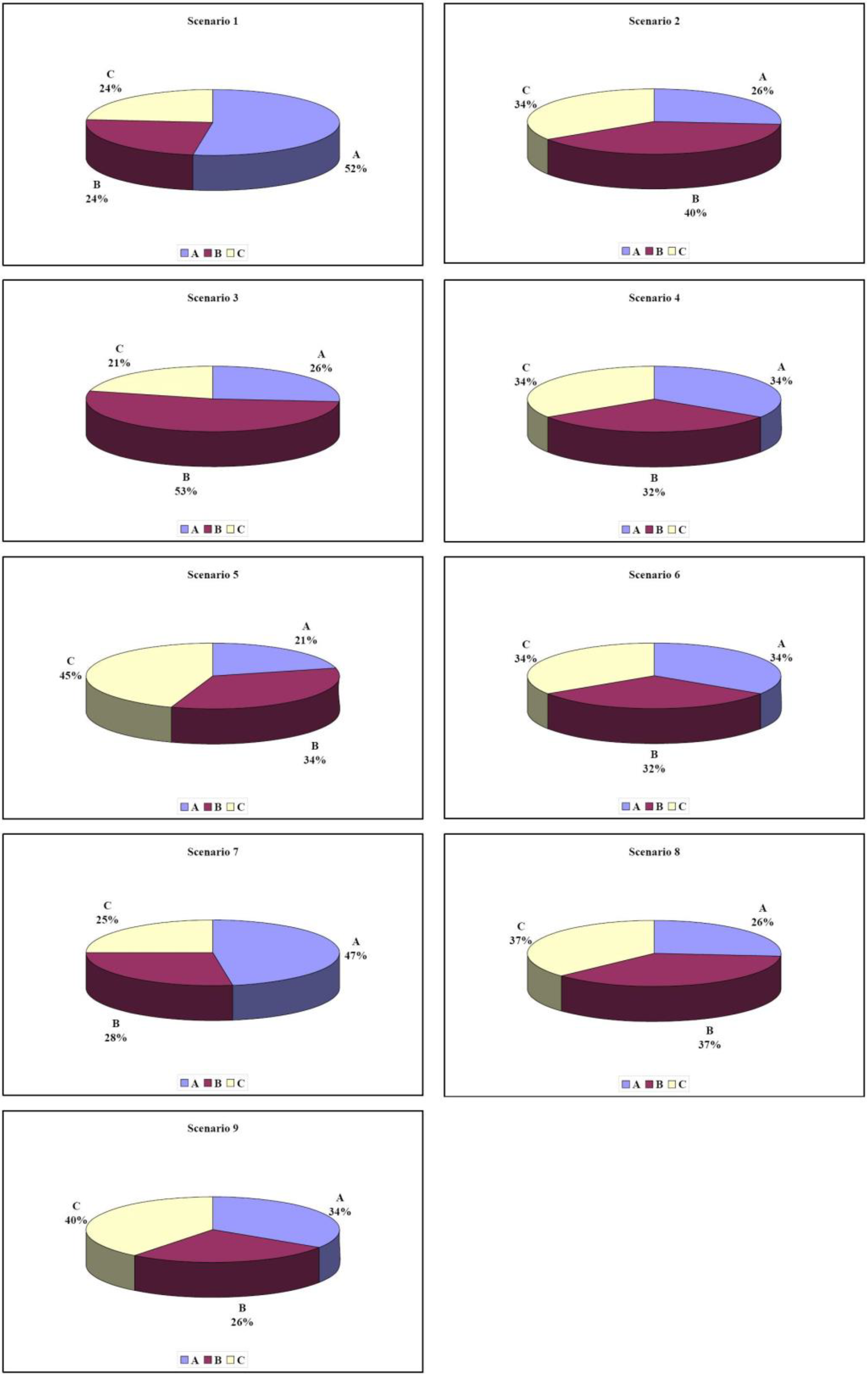
The data and information collected through the questionnaires were analyzed, and the main results are reported in the graphs 2 and 3 that follow (see Figure 2 and Figure 3), each referring to the specific scenario considered.
Analyzing in detail the data shown in the graphs, it is clear that the problem of accessibility (read in terms of access times to the main urban services) as well as the positive environmental characteristics influence the choices, in most cases, with respect to the socioeconomic characteristics for the different alternative urban areas considered. In scenarios 1 and 7, this consideration leads to preferring alternative “A”. On the other hand, the interviewed subjects also showed that they appreciate the improvement of the social characteristics of the context, read in terms of improving safety, accepting modest increases in travel times and, therefore, a slight worsening of accessibility, as well as reductions in the level of environmental characteristics. This determines in the scenarios 2 and 3 a preference for alternative “B”.
Then, there are some cases in which the combination of attribute levels does not lead to identifying a precise alternative of choice (Scenario 4, 6, 8: Alternative “C” and “A”; Alternative “C” and “B”), there being a parity of appreciation among the proposed alternatives, characterized, respectively, by low travel times but by a high degree of environmental characteristics and high travel times with significant increase in social characteristics to the detriment of environmental characteristics.
Finally, in the scenarios where accessibility is very low, the alternative that compensates for this deficiency with high levels of environmental quality and socioeconomic context is preferable. This is evident in scenarios 5 and 9, where alternative “C” is preferred (see Figure 3).
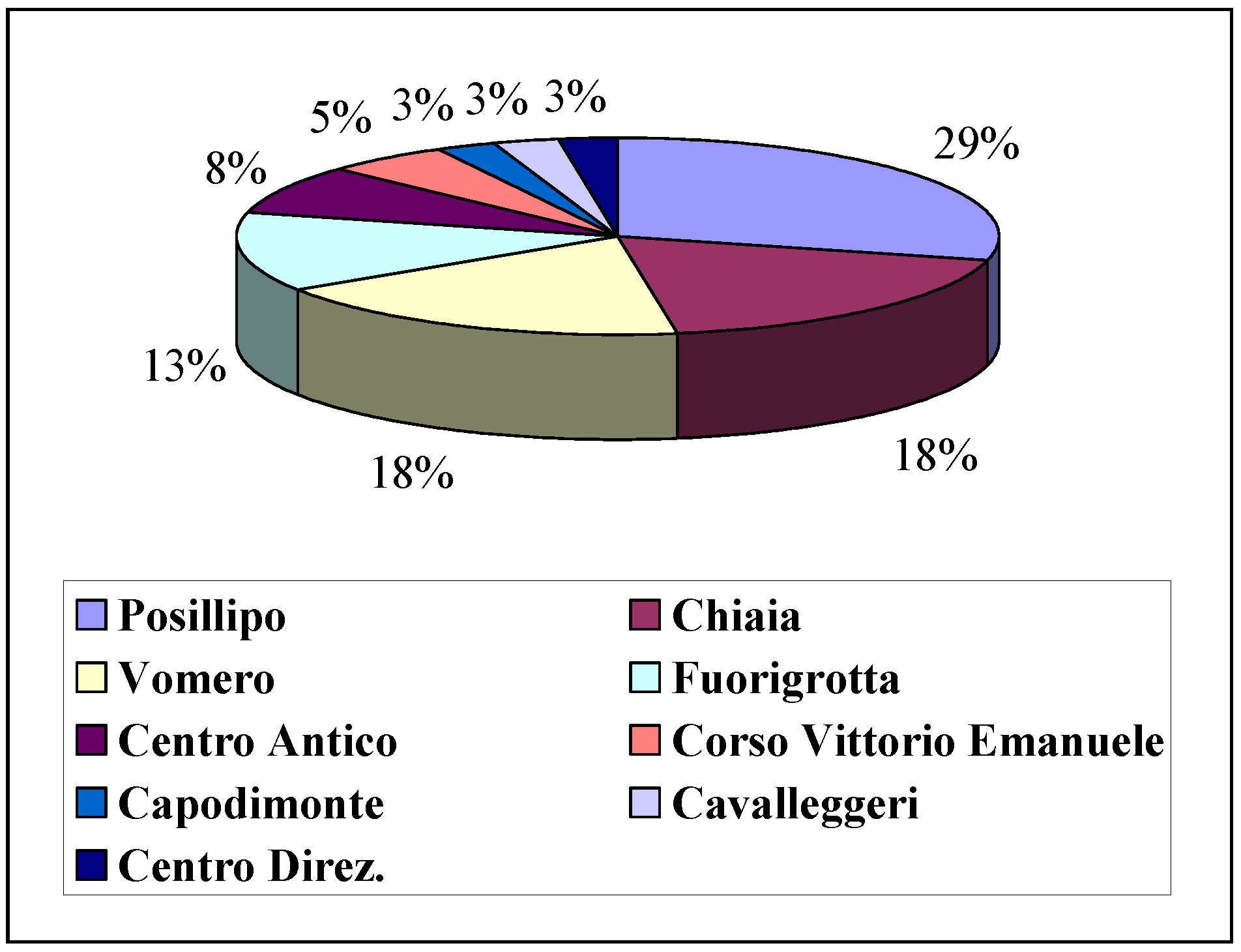
For the purposes of a subsequent testing phase of the proposed model, calibrated on well-defined urban areas of the metropolitan area of Naples, the interviewees were asked to express a preference regarding the possible area in which they would settle among those indicated in the observatory of FIAIP property values (Italian Federation of Professional Real Estate Agents) as homogeneous and isovalue areas of Naples. The preferences therefore revealed that the most appreciated urban areas are those of Posillipo, which has the best environmental qualities and socioeconomic characteristics in spite of a poor accessibility, followed by the Vomero and Chiaia neighborhoods, which instead present, at parity of socioeconomic context, better accessibility but worse levels of environmental quality (see Figure 2).
The following section shows the results obtained with the calibration of the multinomial logit model.
3.4. Step 4: The Multinomial Logit Model
The multinomial logit model represents, today, one of the most widely used random utility models. These models are based on the assumption that the random residuals are all independently and identically distributed (i.i.d.) according to a random Gumbel variable with mean equal to zero and parameter θ, i.e., θi different from zero and equal to [(π2 · θ2)/6] and where for j ≠ i, θi,j is equal to zero (independent alternatives hypothesis), considering the matrix variance/covariance being a diagonal matrix.
Through these assumptions, it can be demonstrated that the probability function in choosing option J, of the set Ii composed of n alternatives, is equal to:
For ease of reference, the preliminary results related to the application and finetuning of the model of selection of the residency are shown in Table 6. The variables examined have already been identified and evaluated in the prior phases of this analysis (see Table 5). From a statistical perspective, the finetuning of the logit model needed to determine the utility function was carried out through the Software BIOGEME 1.7 [65].
According to the indications provided by Kocur et al. in the “Catalogue of computer Program for the Design and analysis of orthogonal Symmetric and Asymmetric Fractional Factorial Experiment, Guide to forecasting travel demand with direct utility assessment”, in correspondence of three variables (each with three levels), the number of required tests to implement the calibration of the model varies between 9 and 27 [64].
Although Table 6 offers a preliminary analysis, its results are consistent with the prior expectations. In fact, the variables “accessibility” and “environmental quality” incorporated under utility terms are positive and have a significant statistical meaning. Likewise, the variable “Social and economic context”, included under dis-utility terms, has a negative sign and also has an acceptable statistical meaning (p-value equal to 0.27). The considerations previously made, relating to the analysis of the scenarios and of Figure 2 and Figure 3, are therefore confirmed (see above) with the substantial validation of the calibration of the logit model.
The results obtained confirm the assumptions on which the model is based and the dynamics of local markets, where the perceived low environmental quality and quality of social decay are characteristic of the urban context examined and strongly affect the selection of the place of residence and, hence, the location of investment in the sector. Even though the survey at hand is a first application on a limited sample of interviewed people (38 subjects for 337 observations in total), the results obtained seem favorable and confirm the validity of the approach used.
4. Conclusions and Further Development
This study represents the first step of a research project to develop a random utility model for the location of real estate investments. The positive results obtained, in particular the selected variables in the case of housing choice, are representative of categories of small owners and tenants. The SP survey conducted was a preliminary pilot study conducted in order to finalize the questionnaire for the assessment of alternative choices. The choice of attributes appears consistent with the dynamics of the local real estate market in which the analysis was carried out. The approach used is appropriate to determine the elements of perception that characterize the problem. In addition, the SP helped us to select, by means of a fractional factorial design, the scenarios to be evaluated and enabled us to gather useful information for the final version of the questionnaire in future experiments.
The next step of the work will be to administer the final questionnaire (developed after the SP study, e.g., a decisional sequential tree can be considered), to a sufficiently broad sample of respondents (the minimum sample size varies from a minimum of 150 to a maximum of 1200 interviews). The choice model will then be calibrated on the basis of a multinomial logit model for the definition of the coefficients of the variables. On the basis of an extended multinomial logit model, we can then also derive a measure of the likelihood of choosing the various investment alternatives of investment, with reference to the different scenarios proposed, assuming independent alternatives for the choice options.
Author Contributions
The work is attributed in equal parts among the authors.
Funding
This research received no external funding.
Conflicts of Interest
The authors declare no conflict of interest.
References
- Del Giudice, V.; Salvo, F.; De Paola, P. Resampling techniques for real estate appraisals: Testing the bootstrap approach. Sustainability 2018, 10, 3085. [Google Scholar] [CrossRef]
- Del Giudice, V.; De Paola, P.; Forte, F. The appraisal of office towers in bilateral monopoly’s market: Evidence from application of Newton’s physical laws to the directional centre of Naples. Int. J. Appl. Eng. Res. 2016, 11, 9455–9459. [Google Scholar]
- Del Giudice, V.; De Paola, P. Undivided real estate shares: Appraisal and interactions with capital markets. Appl. Mech. Mater. 2014, 584–586, 2522–2527. [Google Scholar] [CrossRef]
- Del Giudice, V.; De Paola, P.; Cantisani, G.B. Valuation of real estate investments through Fuzzy Logic. Buildings 2017, 7, 26. [Google Scholar] [CrossRef]
- Del Giudice, V.; De Paola, P.; Forte, F.; Manganelli, B. Real estate appraisals with Bayesian approach and Markov Chain Hybrid Monte Carlo Method: An application to a central urban area of Naples. Sustainability 2017, 9, 2138. [Google Scholar] [CrossRef]
- Del Giudice, V.; De Paola, P. Spatial analysis of residential real estate rental market. In Advances in Automated Valuation Modeling; d’Amato, M., Kauko, T., Eds.; Studies in System, Decision and Control; Springer: Berlin, Germany, 2017; Volume 86, pp. 9455–9459. ISSN 2198-4182. [Google Scholar] [CrossRef]
- Forte, F.; Antoniucci, V.; De Paola, P. Immigration and the Housing Market: The Case of Castel Volturno, in Campania Region, Italy. Sustainability 2018, 10, 343. [Google Scholar] [CrossRef]
- Del Giudice, V.; De Paola, P.; Torrieri, F. An Integrated Choice Model for the Evaluation of Urban Sustainable Renewal Scenarios. Adv. Mater. Res. 2014, 1030–1032, 2399–2406. [Google Scholar] [CrossRef]
- Barreca, A.; Curto, R.; Rolando, D. Assessing Social and Territorial Vulnerability on Real Estate Submarkets. Buildings 2017, 7, 94. [Google Scholar] [CrossRef]
- Fregonara, E.; Rolando, D.; Semeraro, P.; Vella, M. The impact of Energy Performance Certificate level on house listing prices. First evidence from Italian real estate. Aestimum 2014, 65, 143–163. [Google Scholar]
- Oppio, A.; Torrieri, F.; Dell’ Oca, E. Il Valore Delle Aree nel Negoziato Pubblico-Privato: Aspetti Metodologici e Orientamenti Operativi, Valori e Valutazioni; DEI Tipografia del Genio Civile: Roma, Italy, 2018. [Google Scholar]
- Oppio, A.; Torrieri, F. Public and Private Benefits in Urban Development Agreements. In Smart and Sustainable Planning for Cities and Regions; Springer: Berlin, Germany, 2018. [Google Scholar]
- Torrieri, F.; Batà, A. Spatial Multi-criteria Decision Support System and Strategic Impact Assessment: A case study. Buildings 2017, 7, 96. [Google Scholar] [CrossRef]
- Torrieri, F.; Grigato, V.; Oppio, A. A multi methodological model for supporting the economic feasibility analysis for the renovation of the Valsesia railway system. Techne 2016, 11, 135–142. [Google Scholar] [CrossRef]
- Oppio, A.; Torrieri, F.; Bianconi, M. Land value capture by urban development agreements: The case of lombardy region (Italy). In Smart Innovation, Systems and Technologies; Springer: Berlin, Germany, 2018; pp. 346–353. [Google Scholar]
- Morano, P.; Tajani, F.; Locurcio, M. GIS application and econometric analysis for the verification of the financial feasibility of roof-top wind turbines in the city of Bari (Italy). Renew. Sustain. Energy Rev. 2017, 70, 999–1010. [Google Scholar] [CrossRef]
- Morano, P.; Locurcio, M.; Tajani, F.; Guarini, M.R. Fuzzy logic and coherence control in multi-criteria evaluation of urban redevelopment projects. Int. J. Bus. Intell. Data Mining 2015, 10, 73–93. [Google Scholar] [CrossRef]
- Malerba, A.; Massimo, D.E.; Musolino, M.; Nicoletti, F.; De Paola, P. Post Carbon City: Building Valuation and Energy Performance Simulation Programs, Smart Innovation, Systems and Technologies; Springer: Berlin, Germany, 2019; Volume 101, pp. 513–521. [Google Scholar]
- Massimo, D.E.; Musolino, M.; Fragomeni, C.; Malerba, A. A Green District to Save the Planet, Green Energy and Technology; Springer: Berlin, Germany, 2018; pp. 255–269. [Google Scholar]
- Malerba, A.; Massimo, D.E.; Musolino, M. Valuating Historic Centers to Save Planet Soil, Green Energy and Technology; Springer: Berlin, Germany, 2018; pp. 297–311. [Google Scholar]
- Massimo, D.E. Green building: Characteristics, energy implications and environmental impacts. Case study in Reggio Calabria, Italy. In Green Building and Phase Change Materials: Characteristics, Energy Implications and Environmental Impacts; Nova Science Publishers: Hauppauge, NY, USA, 2015; pp. 71–101. [Google Scholar]
- Massimo, D.E. Valuation of urban sustainability and building energy efficiency: A case study. Int. J. Sustain. Dev. 2009, 12, 223–247. [Google Scholar] [CrossRef]
- Alonso, W. Location and Land Use; Harvard University Press: Cambridge, MA, USA, 1964. [Google Scholar]
- Rex, J.; Moore, R. Race, Community and Conflict: A Study of Sparkbrook; Oxford University Press: Oxford, UK, 1967. [Google Scholar]
- Hoang, H.P.; Wakely, P. Status, quality and the other trade-off towards a new theory of urban residential location. Urban Stud. 2000, 37, 7–35. [Google Scholar]
- Kim, J.H.; Pagliara, F.; Preston, J. The intention to move and residential location choice behavior. Urban Stud. 2005, 42, 1–16. [Google Scholar] [CrossRef]
- Cooper, J.; Ryley, T.; Smith, A. Energy trade-offs and market responses in transport and residential land-use patterns: Promoting sustainable development policy and pitfalls. Urban Stud. 2001, 38, 1573–1588. [Google Scholar] [CrossRef]
- Jangik, J.; Hee-Yeon, L. Understanding residential location choices: An application of the UrbanSim residential location model on Suwon, Korea. Int. J. Urban Sci. 2018, 22, 216–235. [Google Scholar]
- Sener, I.N.; Pendyala, R.M.; Bhat, C.R. Accommodating spatial correlation across choice alternatives in discrete choice models: An application to modeling residential location choice behavior. J. Transp. Geogr. 2011, 19, 294–303. [Google Scholar] [CrossRef]
- Di Pasquale, D.; Wheaton, W.C. Urban Economics and Real Estate Markets; Englewood Cliffs: Prentice Hall, NJ, USA, 1996. [Google Scholar]
- Ciuna, M.; Milazzo, L.; Salvo, F. A Mass Appraisal Model Based on Market Segment Parameters. Buildings 2017, 7, 34. [Google Scholar] [CrossRef]
- Saaty, T.L. Decision Making for Leaders. In The Analytic Hierarchy Process for Decisions in a Complex World, New ed.; RWS Publication: Pittsburgh, PA, USA, 2001. [Google Scholar]
- Saaty, T.L.; De Paola, P. Rethinking Design and Urban Planning for the Cities of the Future. Buildings 2017, 7, 76. [Google Scholar] [CrossRef]
- Pagliara, F.; Preston, J.; Simmonds, D. Residential Location Choice. Models and Applications; Springer: Berlin/Heidelberg, Germany, 2010. [Google Scholar]
- Muth, R.F. Cities and Housing; University of Chicago Press: Chicago, IL, USA, 1969. [Google Scholar]
- Mills, E.S. Studies in the Structure of the Urban Economy; Johns Hopkins University Press: Baltimore, MA, USA, 1972. [Google Scholar]
- Evans, A. The Economics of Residential Location; MacMillan: London, UK, 1973. [Google Scholar]
- Wheaton, W.C. On the optimal distribution of income among cities. J. Urban Econ. 1976, 3, 31–44. [Google Scholar] [CrossRef]
- Modelling the Choice of Residential Location. Cowles Foundation Discussion Papers from Cowles Foundation for Research un Economics, Yale University. Available online: https://econpapers.repec.org/paper/cwlcwldpp/477.htm (accessed on 27 May 2019).
- Bhat, C.R.; Guo, J.Y. A Comprehensive Analysis of Built Environment Characteristics on Household Residential Choice and Auto Ownership Levels. Transp. Res. 2007, 41, 506–526. [Google Scholar] [CrossRef]
- Thill, J.; Wheeler, A. Tree induction of spatial choice behavior. Transp. Res. Rec. 2000, 1719, 250–258. [Google Scholar] [CrossRef]
- McFadden, D.; Cox, M.E. The New Science of Pleasure—Consumer Behaviour and The Measurement of Well-Being; Econometric Society World Congress: London, UK, 2005. [Google Scholar]
- Munda, G.; Nardo, M. Constructing Consistent Composite Indicators: The Issue of Weights; EUR 21834 EN; European Commission: Luxembourg, 2004. [Google Scholar]
- Susilo, Y.O.; Williams, K.; Lindsay, M.; Dair, C. The Influence of Individuals’ Environmental Attitudes and Urban Design Features on Their Travel Patterns in Sustainable Neighborhoods in the UK. Transp. Res. Part D 2012, 17, 190–200. [Google Scholar] [CrossRef]
- Manganelli, B. Real Estate Investing Market Analysis, Valuation Techniques, and Risk Management; Springer International Publishing: Cham, Switzerland, 2015. [Google Scholar]
- Earnhart, E. Combining revealed and stated data to examine housing decisions using discrete choice analysis. J. Urban Econ. 2002, 51, 143–169. [Google Scholar] [CrossRef]
- Gayda, S. Stated preference survey on residential location choice in Brussels. In Proceedings of the 8th World Conference on Transport Research, Antwerpen, Belgium, 14–18 September 1998. [Google Scholar]
- Ortuzar, J.; De, D.; Martinez, F.J.; Varela, F.J. Stated preference in modelling accessibility. Int. Plan. Stud. 2000, 5, 65–85. [Google Scholar] [CrossRef]
- Perez, P.E.; Martinez, F.J.; Ortuzar, J.; De, D. Microeconomic formulation and estimation of a residential location choice model: Implications for the value of time. J. Reg. Sci. 2003, 43, 771–789. [Google Scholar] [CrossRef]
- Walker, B.; Marsh, A.; Wardman, M.; Niner, P. Modelling tenants’ choices in the public rented sector: A stated preference approach. Urban Stud. 2002, 39, 665–688. [Google Scholar] [CrossRef]
- Wang, D.; Li, S.-M. Housing preferences in a transitional housing system: The case of Beijing, China. Environ. Plan. 2004, 36, 69–87. [Google Scholar] [CrossRef]
- Kim, J.-H.; Pagliara, F. And Preston, J. An analysis of residential location choice behaviour in Oxfordshire, UK: A combined stated preference approach. Int. Rev. Public Adm. 2003, 8, 103–114. [Google Scholar]
- Bravi, M.; Gicaccaria, S. La conjoint analysis (CA) nelle valutazioni immobiliari. Aestimum 2006, 48, 39–59. [Google Scholar]
- Rosato, P.; Alberini, A.; Zanatta, V.; Breil, M. Redeveloping derelict and underused historical city areas: Evidence from a survey of real estate developers. J. Environ. Plan. Manag. 2010, 53, 257–281. [Google Scholar] [CrossRef]
- Hunt, J.D. Stated Preference Examination of factors influencing residential attraction. In Residential Location Choice. Models and Applications; Pagliara, F., Preston, J., Simmonds, D., Eds.; Springer: Berlin/Heidelberg, Germany, 2010. [Google Scholar]
- Krishna Sinniah, G.; Zaly Shah, M.; Vigar, G.; TeguhAditjandra, P. Residential Location Preferences: New Perspective. Transp. Res. Proc. 2016, 17, 369–383. [Google Scholar] [CrossRef]
- Forman, E.; Peniwati, K. Aggregating individual judgments and priorities with the Analytic Hierarchy Process. Eur. J. Oper. Res. 1998, 108, 165–169. [Google Scholar] [CrossRef]
- Lancaster, K.J. A new approach to consumer theory. J. Political Econ. 1996, 74, 132–157. [Google Scholar] [CrossRef]
- Louviere, J.J.; Hensher, D.A.; Swait, J.D. Stated Preference Methods: Analysis and Application; Cambridge University Press: Cambridge, UK, 2000. [Google Scholar]
- Cascetta, E. Modelli per i Sistemi di Trasporto—Teoria e Applicazioni; UTET Università: Milano, Italy, 2006. [Google Scholar]
- Hensher, D. Stated preference analysis of travel choices—The state of practice. Transportation 1994, 21, 107–133. [Google Scholar] [CrossRef]
- Pearmain, D.; Swanson, J.; Kroes, E.; Bradley, M. Stated Preference Techniques: A Guide To Practice; Steer Davies Gleave and Hague Consulting Group: London, UK, 1991. [Google Scholar]
- FIAIP. Federazione Italiana Agenti Immobiliari Professionisti; Report Urbano; FIAIP: Roma, Italy, 2017. [Google Scholar]
- Kocur, G.; Adler, T.; Hyman, W.; Aunet, B. Catalogue of Computer Program for the Design and Analysis of Orthogonal Symmetric and Asymmetric Fractional Factorial Experiment, Guide to Forecasting Travel Demand with Direct Utility Assessment; Report UMTA-NH-11-0001-82-1; United States Department of Transportation, Urban Mass Transportation Administration: Washington, DC, USA, 1982.
- Bierlaire, M. An Introduction to BIOGEME. Version 1.7. 2008. Available online: www.biogeme.epfl.ch (accessed on 1 February 2019).
Figure 1.
The integrated methodological approach.
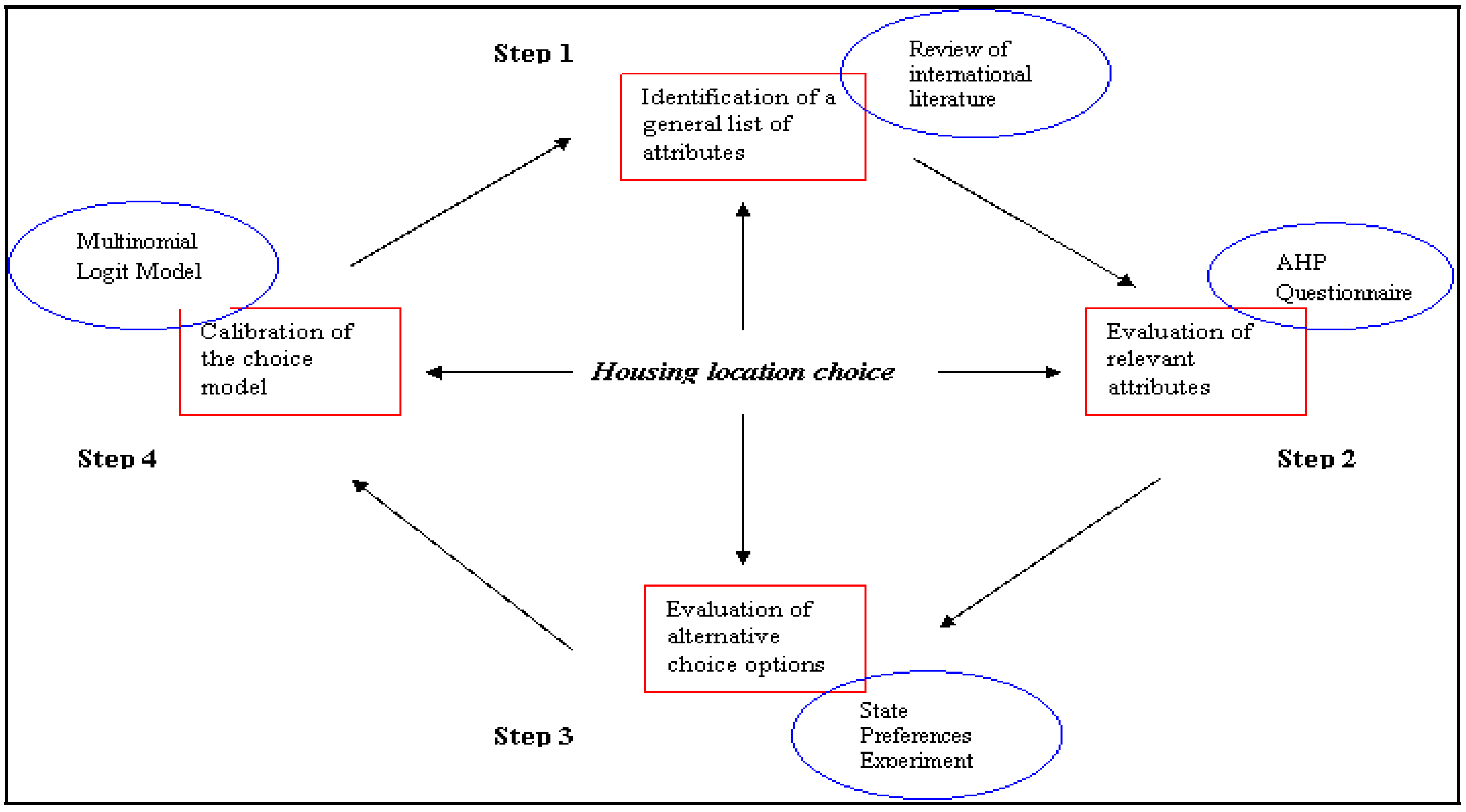
Figure 2.
Preferences related to investment choices for some neighborhoods of Naples.

Figure 3.
Analysis of the scenarios.


Table 1.
Examples of stated preference studies of the housing market [12].
Table 1.
Examples of stated preference studies of the housing market [12].
| Author(s) | Year | Case Study | Explained Variable | Explanatory Variables |
|---|---|---|---|---|
| Cooper et al. | 2001 | Belfast, UK | Housing choice | Density |
| Price | ||||
| Earnhart | 2002 | Fairfield, USA | Housing choice | Dwelling size |
| Natural features | ||||
| Price | ||||
| Gayda | 1998 | Brussel, Belgium | Housing choice | Travel time to work |
| Neighborhood type | ||||
| Housing price | ||||
| Ortuzar et al. | 2000 | Santiago, Chile | Housing choice | Accessibility Location |
| Perez et al. | 2003 | Santiago, Chile | Housing choice | Rent |
| Walker et al. | 2002 | West Midlands, North London, UK | Intention to move | Rent |
| Travel time to work Travel time to education | ||||
| Wang & Li | 2004 | Beijing, PRC | Housing choice | Dwelling attributes Area |
| Rent | ||||
| Neighborhood attributes | ||||
| Kim et al. | 2005 | Oxfordshire, UK | Housing choice Intention to move | House price |
| Travel time to work Travel cost to work Population Density | ||||
| Travel cost to shop | ||||
| School quality | ||||
| Bravi & Giaccaria | 2006 | Torino, Italy | Location choice | Location |
| Typology | ||||
| Price | ||||
| Pollution | ||||
| Subway line | ||||
| Rosato et al. | 2008 | Venezia, Italy | Investment choice | Location Allowable use |
| Access Property regime | ||||
| Presence of conservation restriction | ||||
| Cost per square meter | ||||
| Sener et al. | 2011 | San Francisco Metropolitan Area | Location choice | Location-based accessibility |
| Zonal motorway density | ||||
| Number of household members with work location in 30 min or less by Public Transportation | ||||
| J.D. Hunt | 2010 | Edmonton, Canada | New home alternative | Mobility |
| Traffic noise | ||||
| Municipal taxes or rent | ||||
| Dwelling type | ||||
| Krishna Sinniah, G.; Zaly Shah, M.; Vigar G. | 2016 | Iskandar, Malaysia | Location choice | Neighborhood attributes |
| Sociodemographic characteristics | ||||
| Build environment | ||||
| Accessibility | ||||
| Religious practice | ||||
| Safety and Security | ||||
| Jangik Jin and Hee-Yeon Lee | 2018 | Suwon, Korea | Location choice | Access to employment |
| Average building age | ||||
| Land price | ||||
| Cost to income ratio | ||||
| High residential density Mixed land use |
Table 2.
General list of dwelling attributes.
| Macro-Attributes | Attributes | Description of Attributes |
|---|---|---|
| Characteristics of building | Price | Current market value expressed in Euro/mq |
| Dwelling size | Qualitative parameter defined on 5 classes: Small: up to 45 sqm Middle small: from 45 to 70 sqm Middle: from 70 to 120 sqm Middle great: from 120 to 150 sqm Great: over 150 sqm | |
| Conservation State | Qualitative parameter that indicates the level of degradation related to the maintenance project to be carried out: Low: restructuring construction; Middle: extraordinary maintenance; High: routine maintenance | |
| Style | Presence of decorative elements with historical, artistic or architectural quality | |
| Intrinsic Positional Aspects | Environmental characteristics of real estate (panoramic view, presence of green garden, sunny aspects) expressed using a nominal scale (high, medium, low) | |
| Characteristics of spatial context | Accessibility | Qualitative parameter expressed on the basis of a series of indicators: Proximity to services; Proximity to the workplace; Proximity to schools; Proximity to highways, ports and airports; Quality of public service. The value of the indicator is expressed according to a qualitative scale (high, medium, low) defined in relation to the perception of the respondents concerning their access to the territory where they belong |
| Social and Economic Context | Qualitative parameter defined on the perception of the social and economic context, expressed on the basis of a series of indicators: Safety; Index of allocation of cultural-recreational structures; Index of equipment of education facilities; Index of equipment of health facilities; Index of social infrastructure endowment; Quality of life/liveability. The value of the indicator is expressed on a qualitative nominal scale (high, medium, low) | |
| Environmental Quality | Qualitative parameter linked to the perception of environmental quality in relation to the level of pollution, the presence of public green areas, the presence of parks, etc. The value of the indicator is expressed on a qualitative nominal scale (high, medium, low) | |
| Belonging | Qualitative parameter that aims to represent a sense of belonging to a place associated with the identity of the place |
Table 3.
Weights for groups of respondents.
| Description | Mean 20–35 GR1 | Rank GR1 | Mean 35–50 GR2 | Rank GR2 | Mean 50–65 GR3 | Rank GR3 | |
|---|---|---|---|---|---|---|---|
| Macro attributes | Characteristics of real estate | 0.193 | 2 | 0.185 | 2 | 0.194 | 2 |
| Characteristics of context | 0.730 | 1 | 0.811 | 1 | 0.618 | 1 | |
| Attributes | Characteristics of real estate | ||||||
| Price | 0.130 | 3 | 0.239 | 1 | 0.067 | 6 | |
| Dwelling size | 0.140 | 2 | 0.118 | 4 | 0.137 | 3 | |
| Conservation state | 0.126 | 4 | 0.098 | 5 | 0.100 | 4 | |
| Style | 0.053 | 6 | 0.036 | 6 | 0.085 | 5 | |
| Intrinsic Positional Aspects | 0.281 | 1 | 0.179 | 3 | 0.418 | 1 | |
| Presence of parking | 0.086 | 5 | 0.229 | 2 | 0.180 | 2 | |
| Characteristics of spatial context | |||||||
| Accessibility | 0.142 | 3 | 0.215 | 3 | 0.113 | 3 | |
| Socioeconomic context | 0.182 | 2 | 0.410 | 1 | 0.252 | 2 | |
| Environmental quality | 0.275 | 1 | 0.225 | 2 | 0.441 | 1 | |
| Sense of belonging | 0.117 | 4 | 0.047 | 4 | 0.094 | 4 | |
Table 4.
Aggregate weights for entire group.
| Description | Mean | Rank | |
|---|---|---|---|
| Macro Attributes | Characteristics of real estate | 0.194012 | 2 |
| Characteristics of context | 0.717908 | 1 | |
| Attributes | Characteristics of real estate | ||
| Price | 0.129999 | 4 | |
| Dwelling size | 0.133930 | 3 | |
| Conservation state | 0.109773 | 5 | |
| Style | 0.056238 | 6 | |
| Intrinsic Positional Aspects | 0.279639 | 1 | |
| Presence of parking | 0.155290 | 2 | |
| Characteristics of spatial context | |||
| Accessibility | 0.153775 | 3 | |
| Socioeconomic context | 0.269308 | 2 | |
| Environmental quality | 0.304988 | 1 | |
| Sense of belonging | 0.082376 | 4 | |
Table 5.
Definition of attributes and levels.
| Attribute | Description (Measurement Units) | Level |
|---|---|---|
| Accessibility | Access time from house to the main services and urban infrastructure: in minutes | +5 min +15 min +30 min |
| Environmental quality | Presence of green areas: High = 7–9 Medium = 4–6 Low = 1–3 | High–Medium–Low |
| Socioeconomic context | Safety: High = 7–9 Medium = 4–6 Low = 1–3 | High–Medium–Low |
Table 6.
Model calibration and statistic tests.
| Number of observations | 337 | |||||||||
| Likelihood ratio test | 66,548 | |||||||||
| Rho-square | 0.09 | |||||||||
| Adjusted Rho-square | 0.082 | |||||||||
| Variance-Covariance | from analytical Hessian | |||||||||
| Smallest singular value of the Hessian | 199,992 | |||||||||
| Name of the Variable | β-Value | Std.Err. | t-test | p-value | Robust Std.Err. | Robust t-test | p-value | |||
| Accessibility (A) | 0.0426 | 0.0389 | 1.1000 | 0.2700 | 0.0395 | 1.0800 | 0.28 | |||
| Environmental Quality (EQ) | 0.1480 | 0.0394 | 3.7700 | 0.0000 | 0.0394 | 3.7700 | 0.00 | |||
| Socioeconomic Context (SEC) | −0.1470 | 0.0216 | −6.8200 | 0.0000 | 0.0220 | −6.7100 | 0.00 | |||
| Correlation of coefficients | Coeff1 | Coeff2 | Covariance | Correlation | t-test | p-value | Robust Cov. | Robust Corr. | Robust t-test | p-value |
| A | SEC | −0.0004 | −0.4620 | 3.6200 | 0.00 | −0.0004 | −0.4910 | 3.5300 | 0.00 | |
| A | EQ | 0.0013 | 0.8550 | −5.0300 | 0.00 | 0.0013 | 0.8580 | −5.0300 | 0.00 | |
| EQ | SEC | −0.0005 | −0.5460 | 5.4500 | 0.00 | −0.0005 | −0.5760 | 5.3700 | 0.00 | |
© 2019 by the authors. Licensee MDPI, Basel, Switzerland. This article is an open access article distributed under the terms and conditions of the Creative Commons Attribution (CC BY) license (http://creativecommons.org/licenses/by/4.0/).
Share and Cite
MDPI and ACS Style
Del Giudice, V.; De Paola, P.; Francesca, T.; Nijkamp, P.J.; Shapira, A. Real Estate Investment Choices and Decision Support Systems. Sustainability 2019, 11, 3110. https://doi.org/10.3390/su11113110
AMA Style
Del Giudice V, De Paola P, Francesca T, Nijkamp PJ, Shapira A. Real Estate Investment Choices and Decision Support Systems. Sustainability. 2019; 11(11):3110. https://doi.org/10.3390/su11113110
Chicago/Turabian StyleDel Giudice, Vincenzo, Pierfrancesco De Paola, Torrieri Francesca, Peter J. Nijkamp, and Aviad Shapira. 2019. "Real Estate Investment Choices and Decision Support Systems" Sustainability 11, no. 11: 3110. https://doi.org/10.3390/su11113110
Note that from the first issue of 2016, this journal uses article numbers instead of page numbers. See further details here.