Effectiveness of Diversification Strategies for Ensuring Financial Sustainability of Construction Companies in the Republic of Korea


1
Department of Architectural Engineering, Hanynag University, 222, Wangsipri-ro, Sungdong-gu, Seoul 133-791, Korea
2
Division of Architecture and Civil Engineering, Kangwon National University, 346, Jungang-ro, Samcheok-si, Gangwon-do 25913, Korea
*
Authors to whom correspondence should be addressed.
Sustainability 2019, 11(11), 3076; https://doi.org/10.3390/su11113076
Submission received: 24 April 2019
/
Revised: 26 May 2019
/
Accepted: 27 May 2019
/
Published: 31 May 2019
(This article belongs to the Special Issue Sustainable Business and Development II)
Abstract
:Construction companies recognize diversification as a strategy for ensuring financial sustainability. Hence, the aim of this study was to analyze the dynamic relationship between business diversification and business performance of construction companies using the vector error correction model. The expected default frequency, diversification index, domestic construction order, international construction order, gross Domestic Product, Korea composite stock price index, and interest rate were defined as analytical variables. To derive implications for diversification strategies, construction companies were classified into two groups according to the diversification level, and analyzed from the first quarter of 2001 to the fourth quarter of 2017. The results confirm that the dynamic relationship between the diversification strategy and business performance depends on the diversification level of the company. For changes in the markets entered for diversification, construction companies showed different ways of executing the diversification strategy depending on the group; this was partially because of differences in internal and external capabilities of companies, and each company responded differently to market changes. To ensure financial sustainability of a construction company through effective diversification, various conditions must be considered before deciding what impact the diversification strategy could have on the business performance of the company.
1. Introduction
Financial sustainability is defined as the likelihood that a business is self-sufficient without any external support [1]. To ensure financial sustainability, firms should be able to minimize financial distress due to changes in the internal and external environments [2].
The construction industry is made up of a range of distinctive markets, including new building works, civil engineering, plants, specialist works, repair, maintenance, and decoration [3]. Construction companies are pursuing active changes in entering various construction markets to respond to changes in various internal and external environmental factors. In this constantly changing environment, companies must have appropriate countermeasures to cope with changes to ensure their financial sustainability with a long-term competitive advantage [4,5,6]. In this respect, the most fundamental issue affecting a firm’s business strategy is the process of allocating scarce resources in the face of business constraints and uncertainties [7]. For this reason, many construction companies are diversified, and their diversification is recognized as a corporate strategy for growth and risk management [4].
Business diversification strategies have been defined by various researchers as, among other things, new market entries with new products [8], new approaches to regions and consumers [9], and simultaneous execution of different businesses [10]. In summary, business diversification represents a strategy for executing two or more businesses. In modern portfolio theory, diversification is a way to reduce risk, and risk-averse investors desire to be and are expected to be diversified [11]. However, diversification does not necessarily guarantee the enhanced performance of a company [12]. Quantitative and empirical studies related to the diversification of contractors have often revealed conflicting results about whether or not diversification has a positive effect on the growth, profitability, and stability of companies [13,14,15,16]. The main goals of the business diversification of construction companies are responding to market changes in a stable manner and optimizing return against risk by continuously changing resource allocation among markets based on various construction market situations and internal capabilities of the companies. Financial sustainability of a company refers to its ability to maintain business in a stable manner by efficiently responding to dynamic changes in the market. Thus, business diversification is critical for a construction company to achieve financial sustainability. However, there is a dynamic relationship between diversification and the performance of a construction company due to market changes, but, so far, the existing literature has considered this relationship only to a limited degree.
Therefore, this study aimed to analyze the dynamic relationship between business diversification and business performance of construction companies using the vector error correction model (VECM) and to derive implications for diversification strategies.
2. Literature Review
Studies on diversification have been conducted for many industries and from various perspectives. In such studies, two contradictory theories exist on the effect of the diversification of a company on its value. First, in studies that report that the diversification of a company increases its value, operational efficiency improvement [17,18], improvement in the efficiency of the internal capital market [19,20], and the co-insurance effect [21] are mentioned. Berger et al. (1995) and Chandler (1997) presented an operational efficiency hypothesis that diversified companies are more efficient and profitable than independently operated business sectors because the operational efficiency can be improved through the integration and harmonization of specialized business sectors [17,18]. Weston (1970) mentioned that diversified companies can improve the efficiency of capital allocation by creating internal capital markets by themselves because internal capital markets are more efficient than external capital markets in terms of resource allocation [19]. Moreover, Stulz (1990) argued that diversified companies can efficiently allocate resources and solve underinvestment problems because they can create more efficient capital procurement capabilities than procuring capital from the outside by securing a mutual support system among affiliated companies or businesses [20]. Lewellen (1971) mentioned that companies can decrease profit volatility and thereby reduce their financial risks through diversification, and argued that this leads to an increase in the debt-paying ability compared with non-diversified companies in similar sizes and this again improves the business performance of companies by generating the tax saving effect due to the use of debt [21].
At the same time, the existing literature with the opposite viewpoint claims that business diversification has a negative effect on the business performance of companies due to overinvestment [22], cross-subsidization effect [23], and information asymmetry cost occurrence [24]. Jensen (1986) mentioned that diversified companies can reduce corporate value by arbitrarily allocating resources to execute investment plans that can lower business performance [22]. Meyer et al. (1992) argued that, when resources are transferred among business sectors to assist business sectors with poor business performance, the withdrawal of such businesses is delayed due to the mutual support among business sectors and businesses with negative values persist, thereby reducing the corporate value [23]. Harris et al. (1982) mentioned that a decrease in corporate value is more likely to occur in diversified companies than in non-diversified ones because more cost may be incurred due to the information asymmetry between the management and business sector managers [24].
Such diversification is also being applied to construction companies. Studies on diversification conducted in the construction industries can be divided into studies on diversification strategy and studies on diversification performance measurement. In the construction industry, diversification strategies are being researched mainly for identifying the growth principle of construction companies. Cheah (2002) analyzed the diversification strategies of 21 construction companies conducting business in the international construction market through the market segmentation matrix. The market segmentation matrix presented in the study divides the diversification types of construction companies into project type diversification (e.g., residential buildings, commercial buildings, and industrial facilities), regional diversification (domestic and international), and service diversification (e.g., feasibility study and planning, design, and construction) [25]. Yee et al. (2006a) analyzed the internalization and diversification strategies as well as financial strategies of construction companies for 61 engineering and construction (E&C) companies in the U.S., Europe, Japan, and Korea. As a result, the internationalized companies are characterized by high current ratios and low leverage, and diversified companies have lower current ratios and higher leverage than non-diversified companies [13]. Yee et al. (2006b) studied the relationship among the corporate size, profitability, and diversification strategy for the same companies mentioned in Yee et al. (2006a). As a result, they concluded that small companies have a tendency to concentrate and they enter new markets when their sizes and resources have grown to a certain level [14].
Studies on the diversification performance measurement of the construction industry have been focused on the identification of diversification performance by measuring the diversification levels of companies and quantitatively analyzing the relationship between diversification and business performance.
Choi et al. (2005) analyzed diversification and profitability based on the 12-year data of 59 contractors and 49 non-contractors (e.g., material suppliers, construction engineering companies, and environmental companies) in the U.S. They distinguished specialized companies from diversified companies and analyzed the difference between the two groups, but could not find any important performance difference between the companies with high and low diversification levels [15]. Kim et al. (2012) analyzed the diversification performance of the top 400 construction companies and 500 design companies in the U.S. from 1994 to 2009. They conducted analyses in four areas: diversification and corporate size, diversification and corporate growth, diversification and stability, and corporate growth and corporate size. As a result, they found that large companies are more diversified than small ones, but diversification is not related to the corporate growth rate. Meanwhile, they found that the business performance of the diversified construction companies and design companies is more stable than the standard deviation of the analyzed companies. They concluded that construction companies grow through specialization and they diversify after growth for their safety and survival [16].
Overall, most of the studies on the diversification strategy of construction companies verified the effect of the diversification strategy by conducting regression analysis or variance analysis based on cross-section data. However, as the business performance of construction companies depends on the internal and external business environments changing over time, it appears that dynamic analysis is essential for the diversification strategy. From this perspective, this study was conducted with a focus on the analysis of the dynamic relationship between the business performance and the diversification strategy of construction companies.
3. Methodology
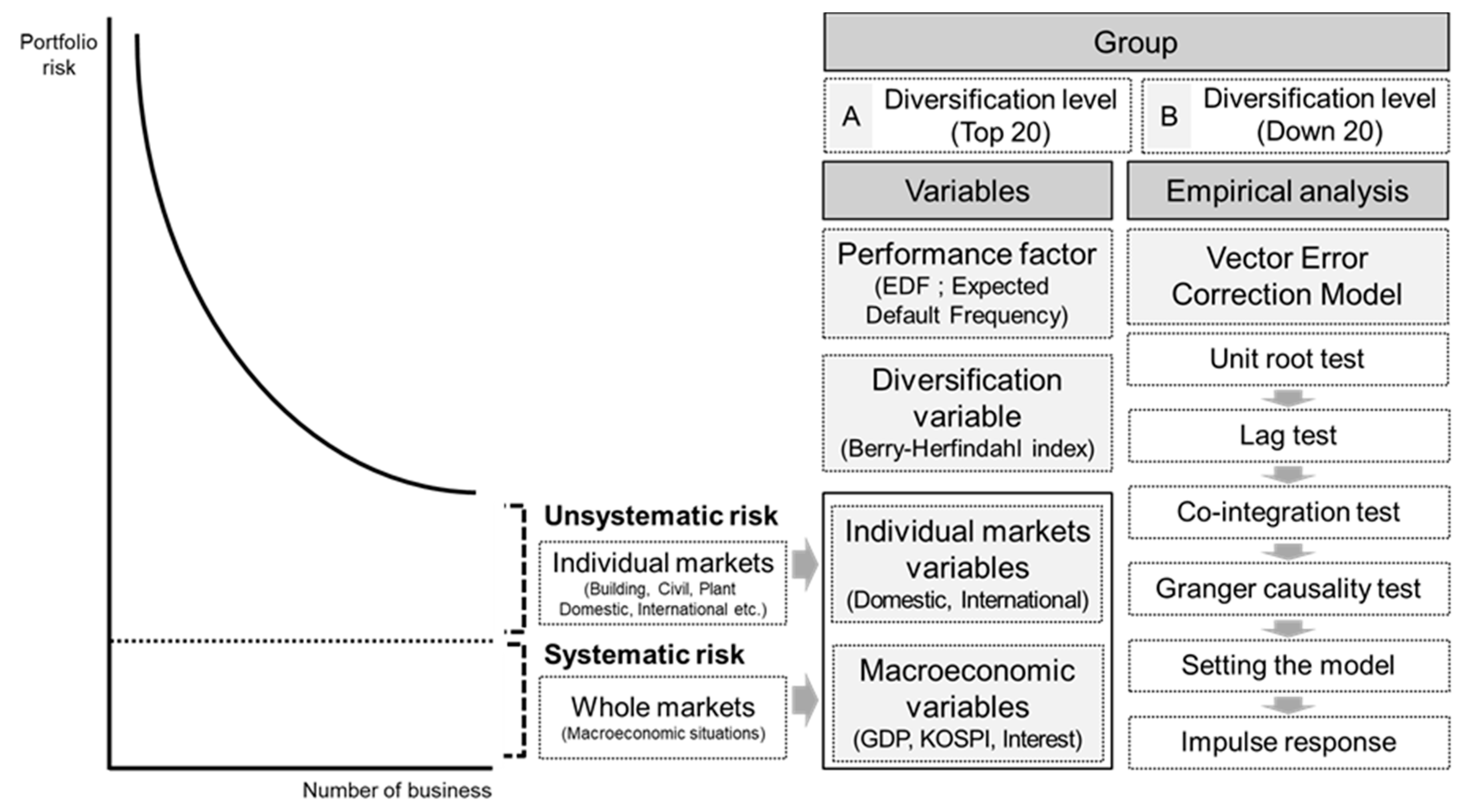
Diversification is based on portfolio theory, in which risk can be largely divided into unsystematic risk and systematic risk. Here, unsystematic risk can be controlled by diversification and is unique to the object of investment, while systematic risk cannot be controlled by diversification and is a risk caused by macroeconomic fluctuations or general market conditions [26]. From this perspective, the dynamic relationship between business diversification and business performance of construction companies was analyzed through the research process in Figure 1 and implications for diversification strategies were derived in this study.
As shown in Figure 1, various macroeconomic variables were used as proxy variables of systematic risk, and individual markets variables were used as proxy variables of unsystematic risk. In other words, as construction companies theoretically perform diversification strategies to efficiently respond to changes in overall and individual markets, analytical variables were selected to reflect the corresponding market changes. To evaluate the diversification level of a company for these market changes, the Berry−Herfindahl index was utilized as a diversification variable. Finally, the expected default frequency (EDF) was defined as the proxy variable for the business performance of a construction company. In general, various financial indicators are used as proxy variables that represent the business performance of a company. EDF, which is calculated based on these financial indicators, has been actively utilized as an index for representing the insolvency level of a company as mentioned above. From this point of view, it appears that EDF can be used to examine changes in the business performance of a company. In this study, the top 20 analyzed companies were set as Group A and the bottom 20 analyzed companies as Group B, based on their diversification level for identifying difference and characteristics of dynamic relationship between business diversification and business performance of construction companies. VECM, a multivariate time series model, was utilized.
3.1. The KMV Model
The Kealhofer, McQuown and Vasicek (KMV) model was constructed based on the structural credit risk measurement model of Black et al. (1973) and Merton (1974) [27,28]. Crosbie et al. (2001) explained the construction of the KMV model and the calculation of EDF in detail [29]. In a model developed by Merton (1974), EDF was calculated using the default distance (DD) normal cumulative distribution function, but the KMV model performed mapping with the historical default frequency in a nonparametric manner. DD is the number expressed with the standard deviation of the average asset value after a year from the default point (DP). Moody’s KMV named the result calculated by mapping the historical default distance with the default frequency as EDF [29]. EDF calculated through the KMV model has superior fitness to other models, and the fitness of the credit measurement results can be improved by simultaneously utilizing EDF with other models. Accordingly, the KMV model is a default prediction model widely used in the financial industry, and 40 out of 50 large financial companies worldwide are using the KMV model [30].
To calculate EDF, the corporate asset value () and the variability of corporate asset value () are first calculated using Equations (1)–(4). The default point (DP) is then calculated using Equation (5). DP represents a point at which a company cannot repay its debt on the due date. In other words, as the KMV model determines a default if the corporate asset value is lower than DP, DP must be calculated. DP is calculated by combining long-term and short-term debts.
Next, the distance to default (DD) must be determined using Equation (6). DD is a value that represents the distance from the insolvency risk considering the variability of corporate asset values and the growth rate of return on asset. By substituting the DD value into the cumulative probability distribution model shown in Equation (7), EDF can be calculated. In other words, the EDF value varies depending on the DD value from the insolvency risk.
where is the corporate stock value, is the corporate asset value, is the total book value of liabilities, is the risk-free rate, is the variability of corporate asset values, is the liability redemption period, is the cumulative distribution function of normal distribution, is the stock value variability, is the corporate short-term liability, is the corporate long-term liability, and is the growth rate of return on asset.
Berndt (2007) mentioned that EDF is useful as a proxy variable for representing the insolvency level of a company [31]. From this perspective, Berndt et al. (2005) stated that they were developing an advanced default prediction model using EDF as a variable for representing the insolvency level of a company [30]. Using a regression analysis of macroeconomic variables and the bank business EDF, Souto et al. (2009) showed that the EDF of individual banks increased as the systematic risk increased [32]. Vassalou et al. (2004) were the first to use the KMV model to compute monthly default likelihood indicators for individual firms, and they examined the effect that default risk has on equity returns [33].
From this perspective, an empirical analysis was conducted in this study by defining EDF calculated through the KMV model as a proxy variable for representing the business performance level of a construction company.
3.2. The Berry−Herfindahl Index
This study used the diversification index as a proxy variable in estimating unsystematic risk. The most common method of identifying the diversification level in a company’s business portfolio is by using the Berry–Herfindahl index [34]. It relies on a classification system to assess the extent of a firm’s operations in different classified groups. The modified Berry–Herfindahl index can be defined as follows:
where mij is the proportion of the jth classified group in the ith firm’s total sales, and M is the number of classified groups in which a firm operates. From this measure, if a firm operates in a single classified group, the Berry–Herfindahl index of diversification is 0 and it comes close to 1 if the firm’s total sales are divided equally among any number of classified groups [35].
Although the Berry–Herfindahl index is a single variable, it has been used as an analytical variable in various studies due to its usefulness. Lang et al. (1994) confirmed that Tobin’s q of diversified companies is smaller than Tobin’s q constructed by the matching portfolio composed of specialized companies using the Berry–Herfindahl index [36]. Berger et al. (1995) estimated the effect of diversification on firm value by imputing stand-alone values for individual business segments using the Berry–Herfindahl index [17]. Comment et al. (1995) analyzed the relationship between corporate concentration and corporate performance for approximately 2000 companies from 1978 to 1989 [37]. As seen, the Berry–Herfindahl index has been used as a proxy variable for representing the diversification level of a company in various studies. Therefore, the Berry–Herfindahl index was also used as a variable for representing the business diversification of a construction company in this study.
3.3. The Vector Auto-Regression (VAR) Model
In this study, an empirical analysis was conducted through VECM. Unlike general structural models, the vector auto-regression (VAR) model is a multivariate time series model constructed using the correlations and lag correlations between variables while transcendental economic theories are excluded [38]. The VAR model can use the structural relationships between the variables in the model without losing practically useful information because specific economic theories are not restricted. In other words, the VAR model can be said to be a dynamic model in which variables affect one another for the analysis of multiple time series data [39].
The VAR model consists of n linear regression equations, and each equation sets the currently observed values of the variables with causal relationships with one another as dependent variables and the values of the variables observed in the past as explanatory variables. In general, for N × 1 (vector) macroeconomic variables, Yt, the VAR model with lag p can be expressed with the following regression equation: Yt represents N × 1 (vector) macroeconomic variables, αt the coefficient matrix, and et the probabilistic error term; L, a lag operator, represents L1Yt = Yt − 1, L2Yt = Yt − 1, …; and A(L) = A1L1 + A2L2 + A3L3 + …. [40].
When the time series data of the VAR model are non-stationary, level variables are subjected to differencing and used for the analysis. In this instance, the unique information of the level variables can be lost. In this case, analysis can be conducted using VECM if there is a long-term relationship between the non-stationary level variables, i.e., co-integration [41]. VECM is a limited form of the VAR model used when there is co-integration. It can be written as a dynamic model considering the co-integration relationship between time series with other short-term dynamic relationships:
where β is the (n × r) matrix representing the co-integration relationship. The β’Xt-p term, which represents r linear combinations, is the unbalanced error at time point t-p. This unbalanced error affects {Xt} at the next time point t due to the coefficient α. Owing to this, the (n × r) coefficient matrix α is referred to as an error correction coefficient. In this study, the co-integration test was conducted and it was found that co-integration existed. Therefore, an empirical analysis was conducted using VECM.
4. Empirical Analysis
4.1. Variables and Data Collection
For the purpose of analyzing the relationship between business performance and diversification strategies of construction companies, in this study, EDF was used as a proxy variable for representing business performance of a construction company. In general, various financial indicators are used as proxy variables for representing the business performance of a company. EDF calculated based on such financial indicators is being actively used as an index for representing the insolvency level of a company, as mentioned above. From this perspective, it appears that EDF can be used to examine changes in the business performance of a company. Moreover, in this study, the Berry−Herfindahl Index was used as a proxy variable for representing the diversification level of a construction company. For unsystematic risk, the domestic and international construction orders were defined as proxy variables for representing individual market situations. There are various individual market variables by work type and region, but it appears that domestic and international market situations have the most differentiated characteristics. Therefore, these two corresponding variables were defined as individual market variables. Moreover, for systematic risk, the gross domestic production (GDP), Korea composite stock price index (KOSPI), and interest rate were defined as proxy variables for representing macroeconomic situations. Table 1 shows the previous studies that utilized macroeconomic variables. As shown in the table, GDP, the stock price index, variables related to construction markets (e.g., construction producer price index, building cost index, and construction output), and interest rate, which were used in this study, as well as various variables, such as the unemployment rate, consumer price index, housing price index, and money supply, were utilized. In this study, among these various macroeconomic variables, the variables judged to be overlapping in explaining the effects on the business performance of construction companies were excluded. In other words, the unemployment rate and consumer price index, among others, were excluded because they are variables for representing overall market situations including construction markets and their effects can be included in the effects of GDP, KOSPI, and interest rate. Furthermore, as money supply represents the liquid fund that can be invested in the construction market, it appears that it can be replaced with construction orders. In addition, since KOSPI was used as a variable for representing the equity market, which is a representative investment market where money supply is introduced, the relationship between the real estate market and the financial market was also considered. The interest rate was used as a variable because real estate investment is performed mostly through loans.
Table 2 shows descriptions of variables. In this study, to calculate EDF, 40 construction companies currently listed on the stock market within the 200th ranking in the 2018 construction capability evaluation in Korea were selected as samples for analysis. After the diversification index of each sample was calculated, the top 20 construction companies were set as Group A and the bottom 20 companies as Group B based on the diversification level. The EDF of each company was measured over time, and the average values at each time point were calculated. The derived average EDF values for each group were used as the time series data of construction company business performance variables of the corresponding groups. Moreover, the time series data for the diversification index of each group were also calculated using the average values at each time point. Multiple variables are needed to measure the EDF, such as asset value variability, asset value, default point, risk-free interest rate, and average return on asset. This study used the interest rate of three-year term government and public bonds as the risk-free interest rate, and used the total return on asset from the financial ratio as the average return on asset. In addition, asset value, asset value variability, and default point were calculated using formulas. The domestic construction order, international construction order, GDP, KOSPI, and interest rate were obtained from the data of Statistics Korea. The time-series data in this study were quarterly data from Q1 of 2001 to Q4 of 2017.
4.2. Unit Root Test
When series analysis is conducted, stationary series data must be used. If series analysis were conducted using non-stationary serial data, the spurious regression phenomenon, in which non-correlated variables appear to be highly related, would occur [48]. To test whether the serial data are stationary, the existence of the unit root in the serial data must be examined. The existence of the unit root represents that the serial data are non-stationary. In this study, to test whether serial data are stationary, the augmented Dickey–Fuller (ADF) test, which is a representative unit root test, was utilized. Table 3 shows the results of the unit root test. As most of the DF-t statistical values were larger than 1%, 5%, and 10% significance levels for both Groups A and B in the case of level variables, the null hypothesis that the unit root exists could not be rejected in most cases. When the level variables of Groups A and B were subjected to the first differencing and the unit root test was conducted, however, the null hypothesis that the unit root exists was rejected at 1%, 5%, and 10% significance levels. This means that the variables subjected to the first differencing were stationary.
4.3. Cointegration Test
If the traditional regression analysis method were applied to the variables that were considered to be non-stationary time series by the unit root test, spurious regression problems would occur. Despite non-stationary time series, however, the results of the traditional regression analysis can be meaningful if there is a co-integration relationship between them. If co-integration exists, VECM must be used for the analysis [49].
To conduct the cointegration test, a test on the optimal lag was conducted first. As the VAR model produces errors when the lag length is set arbitrarily, optimal lag must be tested by the information theory to secure the reliability of the research. In general, the p lag of the VAR(p) model is determined through the Akaike information criteria (AIC) and the Schwarz information criteria (SIC) methods, and the minimized values based on each criterion are determined to be the optimal lags. The derived optimal lags increase the explanatory power of the model when new variables are introduced, but they increase the size of the model at the same time and thus reduce the degrees of freedom. Therefore, a smaller lag is chosen to secure the simplicity of the model [50]. Accordingly, in this study, the optimal lags were tested as shown in Table 4 and lag 1 was determined to be the optimal lag for both Groups A and B based on the SIC criterion.
Based on this, the Johansen test method, a representative co-integration test method, was conducted in this study as shown in Table 5. As a result, it was found that there was a co-integration relationship at the 5% significance level because the null hypothesis that “the number of co-integration vectors is r or less” was rejected. As it was confirmed that there was a co-integration relationship between the level variables, analysis was conducted through VECM.
4.4. Granger Causality Test
In the VAR model, different analysis results are derived depending on the arrangement sequence of endogenous variables. Therefore, the arrangement sequence of the variables must be determined according to the causal relationship before constructing the VAR model. For this, the Granger causality test was conducted in this study. The Granger causality test is a method for clearly distinguishing antecedents from consequences using the lag distributed model, whereas economic theories are excluded [51]. As shown in Table 6 and Table 7, the causality was set based on the p-value of the causality between the variables by conducting the Granger causality test for various lags. As a result, the analysis model was set by arranging the variables in the order of: It ▷ GDPt ▷ KOSPIt ▷ Intert ▷ Domet ▷ EDFt ▷ Divt for Group A; and GDPt ▷ It, ▷ Divt ▷ EDFt ▷ KOSPIt ▷ Intert ▷ Domet for Group B.
5. Results
In this study, an impulse response analysis, based on the test results above, was performed by creating a VECM. The impulse response analysis presents a study of the correlations between the variables and their ripple effects by examining the fluctuations in the variables in the model themselves and other variables over a certain period of time when the impact of one standard deviation is applied to the variables in the model [52]. In this study, the dynamics of variables within the model were analyzed, after giving a certain impulse to EDF, diversification index, and macroeconomic variables through the impulse response analysis.
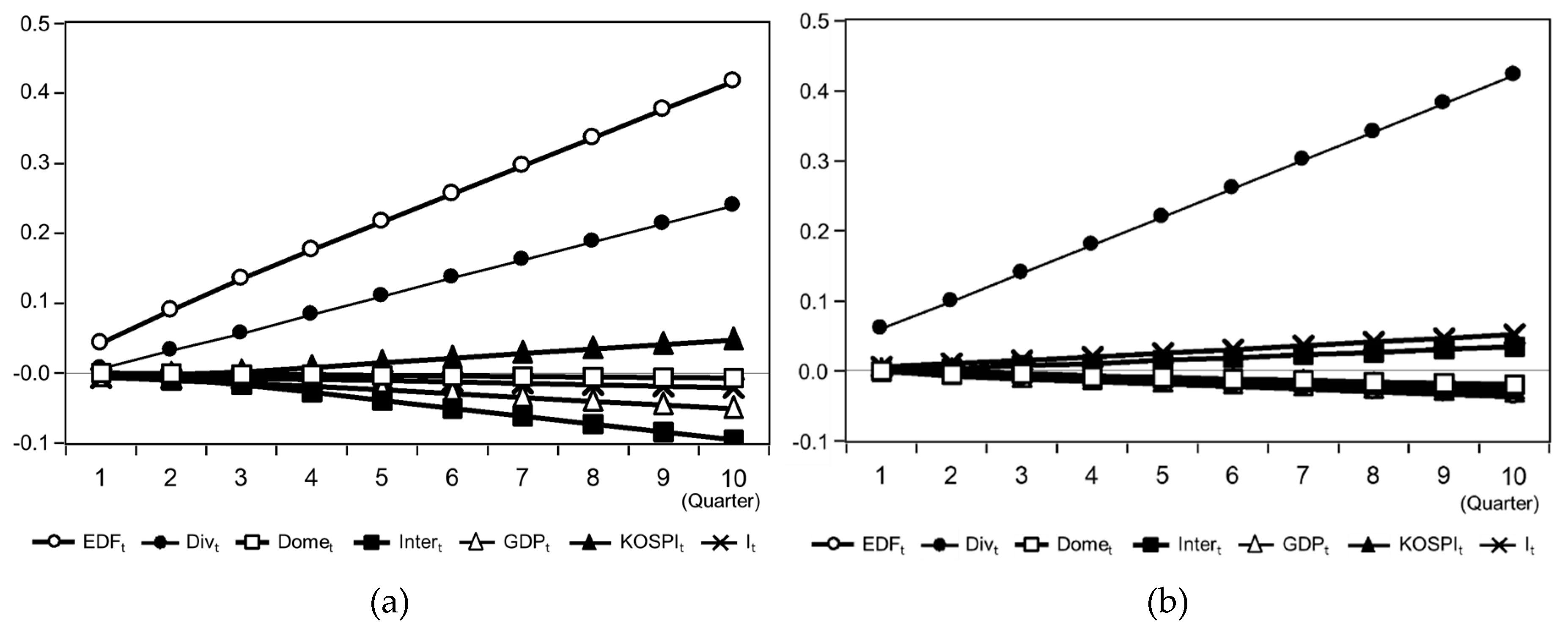
First, Figure 2 and Table 8 show the dynamic relationships among EDF, diversification index, individual market variables, and macroeconomic variables in Group A. EDF fluctuated in the positive direction in response to the EDF impulse, and its fluctuation width was the largest. In response to the diversification index impulse, EDF fluctuated in the negative direction at the beginning, but the fluctuation direction changed to the positive direction over time. EDF fluctuated in the negative direction in response to the domestic construction order impulse, but it fluctuated in the positive direction in response to the international construction order impulse. Moreover, EDF fluctuated in the negative direction in response to the GDP and KOSPI impulses, but it generally fluctuated in the positive direction in response to the interest impulse. The diversification index fluctuated in the positive direction in response to the diversification index and EDF impulses. The diversification index fluctuated in the positive direction in response to the domestic construction order impulse. In response to the international construction order impulse, the diversification index went through changes in the fluctuation direction but it gradually fluctuated in the negative direction. Moreover, the diversification index fluctuated in the negative direction in response to the GDP and interest impulses, but it fluctuated in the positive direction in response to the KOSPI impulse.
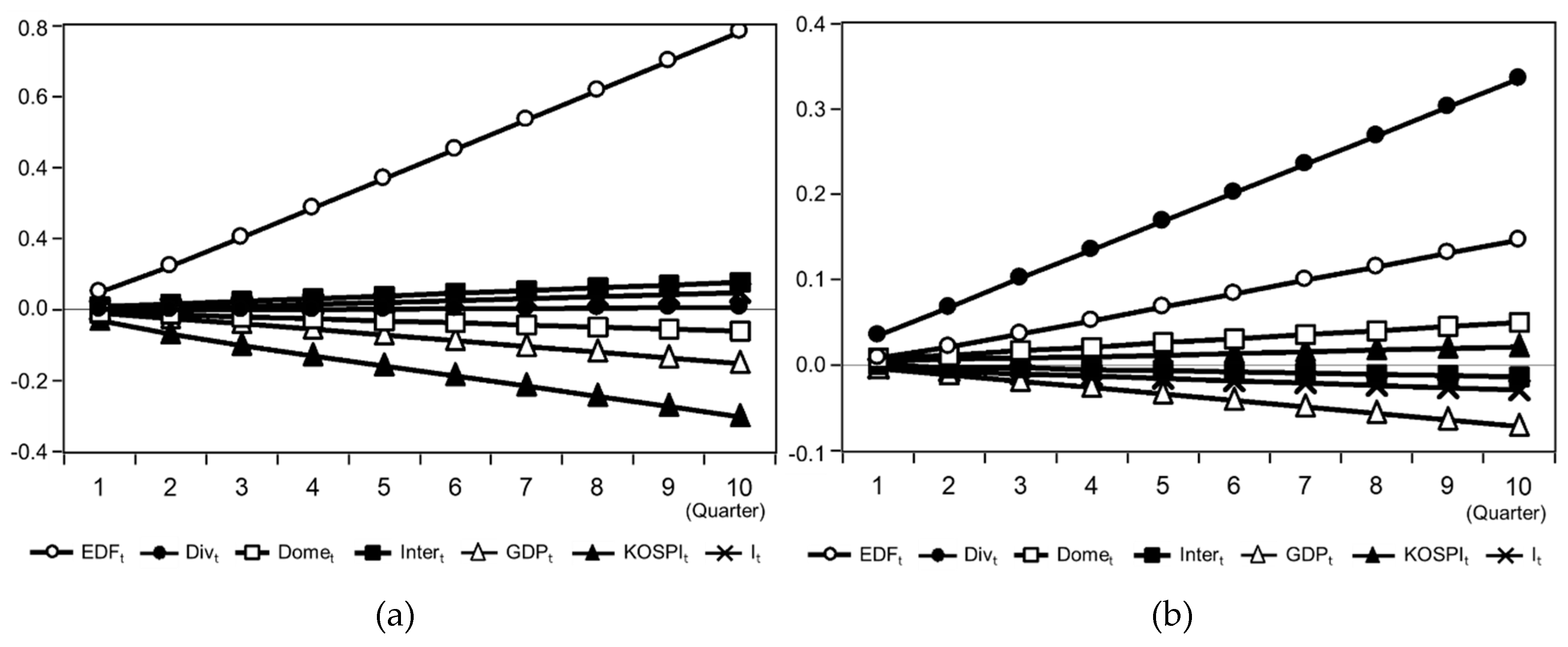
As shown in Figure 3 and Table 9, the dynamic relationships among the variables in Group A through the cumulative impulse response function also show similar results as described above.
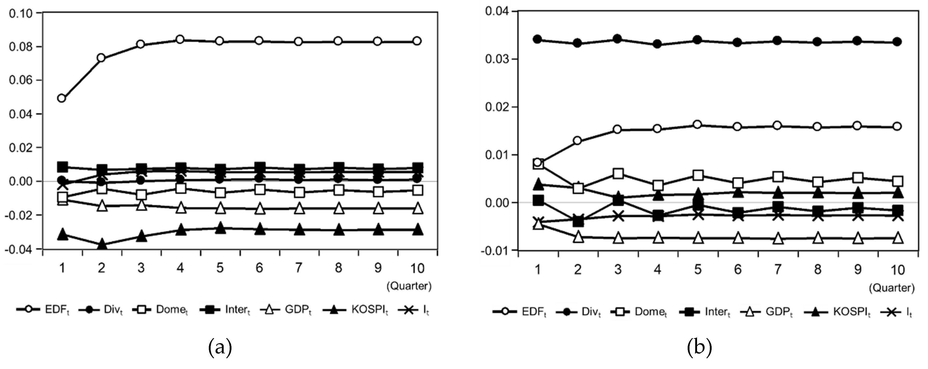
Next, Figure 4 and Table 10 show the dynamic relationship between EDF, diversification index, individual market variables, and macroeconomic variables in Group B. EDF fluctuated in the positive direction in response to the EDF and diversification index impulses. EDF fluctuated in the negative direction in response to the domestic construction order and international construction order impulses. Moreover, EDF fluctuated in the negative direction in response to the GDP and interest impulses. In response to the KOSPI impulse, EDF went through a change in the fluctuation direction and gradually fluctuated in the positive direction. The diversification index fluctuated in the positive direction in response to the diversification index impulse, but it fluctuated in the negative direction in response to the EDF impulse. In response to the domestic construction order impulse, the diversification index went through changes in the fluctuation direction, but it gradually fluctuated in the negative direction. In response to the international construction order impulse, the diversification index fluctuated in the positive direction. Finally, the diversification index fluctuated in the negative direction in response to the GDP and KOSPI impulses, but it fluctuated in the positive direction in response to the interest impulse. Furthermore, as shown in Figure 5 and Table 11, the dynamic relationships among the variables in Group B through the cumulative impulse response function show similar results as described above.
Summarizing these findings, the following results can be derived. First, it was found that the construction companies with relatively higher diversification indices in Group A could improve their business performance through diversification, but the effect was not uniform. For the companies with lower diversification indices in Group B, their business performance decreased as the diversification index increased. As there are various construction markets by work type and region, companies with low diversification indices show a tendency to be specialized in and focused on specific markets. As this indicates that they lack business networks, skills, and capabilities to enter other markets, performing diversification while they are not prepared has a negative impact on their performance. Moreover, companies with high diversification indices have the effect of diversification. As markets continuously change over time, however, the effect of diversification can be secured by predicting market changes in advance and continuously managing their business portfolios.
Second, when the business performance of the companies deteriorated, the diversification index showed a tendency to increase for the construction companies with high diversification indices but it showed a tendency to decrease for the construction companies with low diversification indices. This appears to be because the construction companies with low diversification indices executed business concentration strategies to improve their business performance as they have capabilities specialized in specific work types and regions while the companies with high diversification indices improved their business performance using various business networks for the entire construction market.
Third, regarding changes in the business performance of construction companies caused by the impulses of individual market variables, the increase in the domestic or international construction order had a positive impact on the business performance of construction companies with low diversification indices. However, the increase in the international construction order had a negative impact on the business performance of construction companies with high diversification indices. The fact that the risk of the international construction market is higher than that of the domestic market has been mentioned in previous studies [5,53]. In other words, construction companies grew based on the domestic construction market and then entered the international construction market with different environments and various risks, but such multinational diversification had a negative impact on their business performance. Moreover, this tendency was more obvious for the companies with high diversification indices than for the companies with low diversification indices because the size of the international construction order was relatively larger.
Fourth, the companies with high diversification indices showed a negative relationship between the international construction order and the diversification index but a positive relationship between the domestic construction order and the diversification index. At the same time, the companies with low diversification indices showed an opposite tendency. As the companies with low diversification indices focused their business on the domestic construction market, the increase in the diversification index with the increase in the international construction order and the decrease in the diversification index with the increase in the domestic construction order are reasonable results. For the companies with high diversification indices for which business proportions were relatively evenly distributed, however, the diversification index showed a tendency to decrease as the domestic construction order decreased. This appears to be because they attempted to improve their business performance in the international construction market when the domestic construction market was in recession.
6. Discussion and Conclusions
In this study, the dynamic relationship between business diversification and business performance of construction companies was analyzed using VECM, and implications for diversification strategies were derived. The analysis results confirm that it was the companies with high diversification indices that benefited from the diversification strategy. It is necessary, however, to predict market changes in advance and to continuously manage business portfolios for the continuation of the effect of diversification. Moreover, it was found that the construction companies had different ways of executing the business diversification strategy to improve their business performance. In other words, the companies with relatively lower diversification levels showed a tendency to concentrate on businesses they specialized in to improve their business performance while those with high diversification levels utilized the diversification strategy more actively using various business networks.
It was found that entry into individual markets, especially into the international construction market, had a more negative impact on the business performance of the construction companies with higher diversification levels. This appears to be because the international construction business risk was relatively higher even for the companies with relatively higher proportions of entry into the international construction market. It was also found that the companies with high diversification levels sought opportunities in the international construction market when the domestic construction market was depressed. Their practical business performance, however, was not good because the international construction business risk was relatively higher as mentioned above.
Many construction companies use diversification strategies to secure financial sustainability. The diversification levels of companies will be different depending on various capabilities, such as business networks, technologies, and management skills. After all, it is necessary to clearly identify the strengths and weaknesses of individual companies to effectively respond to ever-changing macroeconomics and individual markets. Moreover, if the diversification level is raised through entry into other markets without preparation to secure the survival of a construction company after market changes, the cash flow can be secured at the moment but the deterioration in the profitability will be fatal in the end. In the case of South Korea, when the domestic construction market stagnated due to the global financial crisis of 2008, domestic companies aggressively expanded to overseas construction markets to overcome their liquidity crisis. As a result, they won many projects, but large deficits were generated when the projects were completed, creating serious problems. Companies diversified their businesses in overseas markets, but their low-cost orders, accepted for the sake of survival, had a detrimental impact. In other words, to secure the financial sustainability of a construction company through the effective utilization of diversification strategies, it is necessary to identify the capabilities of the company itself and to gain insight into market changes before deciding whether a diversification strategy is ultimately favorable or unfavorable.
This study derived implications for the diversification strategies of Korean construction companies. Korea, a previously underdeveloped country, has achieved rapid economic growth, and domestic construction companies are striving to expand their business scope to overseas construction markets because the domestic market has remained stagnant. Considering this situation, the dynamic relationships between various market fluctuations and firms’ diversification strategies are expected to provide important business strategies for construction companies in developing countries worldwide. The findings of this study suggest that construction companies in developing countries with growing domestic markets should efficiently use business diversification strategies to achieve financial sustainability. Changing the business area of a company to enable it to cope with the changing dynamics of the construction market can have adverse effects on its business management. Therefore, sustained efforts are needed to predict market fluctuations and to strengthen internal capabilities of firms to efficiently respond to these changes. Such actions will contribute to a construction company’s expansion into diverse markets and minimize the detrimental impact of business diversification.
In this study, the EDF was used as a proxy variable for the business performance of a construction company. However, the EDF, which is based on the KMV model, is limited regarding its applicability to general construction companies, because it is calculated only for companies listed on the stock market. Thus, indices that can effectively represent the business performance of general construction companies need to be analyzed. Furthermore, as mentioned above, an in-depth analysis of measures is required to assist firms in strengthening internal capabilities to secure flexibility of business strategies and to proactively respond to market fluctuations.
Author Contributions
M.H. developed the concept and drafted the manuscript. S.L. revised the manuscript and supervised the overall work. J.K. reviewed the manuscript. All authors read and approved the manuscript.
Funding
This work was supported by the National Research Foundation of Korea (NRF) grant funded by the Korea government (MSIT) (NRF-2018R1A2B6007333).
Conflicts of Interest
The authors declare no conflict of interest.
References
- Iezza, P. Financial Sustainability of Microfinance Institutions (MFIs): An Empirical Analysis. Master’s Thesis, Copenhagen Business School, Copenhagen, Denmark, 2010. [Google Scholar]
- Hu, H.; Sathye, M. Predicting Financial Distress in the Hong Kong Growth Enterprises Market from the Perspective of Financial Sustainability. Sustainability 2015, 7, 1186–1200. [Google Scholar] [CrossRef] [Green Version]
- Ho, P.H.K. Analysis of Competitive Environments, Business Strategies, and Performance in Hong Kong’s Construction Industry. J. Manag. Eng. 2016, 32, 04015044. [Google Scholar] [CrossRef]
- Kim, H.; Reinschmidt, K.F. Association of Risk Attitude with Market Diversification in the Construction Business. J. Manag. Eng. 2011, 27, 66–74. [Google Scholar] [CrossRef]
- Jung, W.; Han, S.H.; Lee, K.W. Country Portfolio Solutions for Global Market Uncertainties. J. Manag. Eng. 2012, 28, 372–381. [Google Scholar] [CrossRef]
- Lee, S.; Tae, S.; Yoo, S.; Shin, S. Impact of Business Portfolio Diversification on Construction Company Insolvency in Korea. J. Manag. Eng. 2016, 28, 05016003. [Google Scholar] [CrossRef]
- Jiang, A.; Malek, M.; El-Safty, A. Business Strategy and Capital Allocation Optimization Model for Practitioners. J. Manag. Eng. 2011, 27, 58–63. [Google Scholar] [CrossRef]
- Ansoff, H.I. Corporate Strategy: Business Policy for Growth and Expansion; McGraw-Hill: New York, NY, USA, 1965. [Google Scholar]
- Steinter, G. Strategic Factors in Business Success; Financial Executives Research Foundation: New York, NY, USA, 1969. [Google Scholar]
- Rumelt, R.P. Strategy, Structure, and Economic Performance; Harvard University Press: Cambridge, MA, USA, 1974. [Google Scholar]
- Rubinstein, M. Markowitz’s Portfolio Selection: A Fifty-Year Retrospective. J. Financ. 2002, 57, 1041–1045. [Google Scholar] [CrossRef]
- Sung, Y.K.; Lee, J.H.; Yi, J.S.; Son, J.W. Establishment of Growth Strategies for International Construction Firms by Exploring Diversification-Related Determinants and Their Effects. J. Manag. Eng. 2017, 33, 04015044. [Google Scholar] [CrossRef]
- Yee, C.Y.; Cheah, C.Y.J. Fundamental Analysis of Profitability of Large Engineering and Construction Firms. J. Manag. Eng. 2006, 22, 203–210. [Google Scholar] [CrossRef]
- Yee, C.Y.; Cheah, C.Y. Interactions between Business and Financial Strategies of Large Engineering and Construction Firms. J. Manag. Eng. 2006, 22, 148–155. [Google Scholar] [CrossRef]
- Choi, J.; Russell, J.S. Long-term entropy and profitability change of United States public Construction firms. J. Manag. Eng. 2005, 21, 17–26. [Google Scholar] [CrossRef]
- Kim, H.; Reinschmidt, K. Market Structure and Organizational Performance of Construction Organizations. J. Manag. Eng. 2012, 28, 212–220. [Google Scholar] [CrossRef]
- Berger, P.G.; Ofek, E. Diversification’s effect on firm value. J. Financ. Econ. 1995, 37, 39–65. [Google Scholar] [CrossRef]
- Chandler, A.D. The Visible Hand: The Managerial Revolution in American Business; Harvard University Press: Cambridge, MA, USA, 1977. [Google Scholar]
- Weston, J.F. The Nature and Significance of Conglomerate Firms. St. John’s Law Rev. 1970, 44, 66–80. [Google Scholar]
- Stulz, R.M. Managerial Discretion and Optimal Financing Policies. J. Financ. Econ. 1990, 26, 3–27. [Google Scholar] [CrossRef]
- Lewellen, W.G. A Pure Financial Rationale for the Conglomerate Merger. J. Financ. 1971, 26, 521–537. [Google Scholar] [CrossRef]
- Jensen, M.C. Agency Costs of Free Cash Flow, Corporate Finance and Takeovers. Am. Econ. Rev. 1986, 76, 323–329. [Google Scholar]
- Meyer, M.; Milgrom, P.; Roberts, J. Organizational Prospects, Influence Costs, and Ownership Changes. J. Econom. Manag. Strategy 1992, 1, 9–35. [Google Scholar] [CrossRef]
- Harris, M.; Kriebel, C.H.; Raviv, A. Asymmetry Information, Incentives and Intra Firm Resource Allocation. Manag. Sci. 1982, 28, 604–620. [Google Scholar] [CrossRef]
- Cheah, Y.J. Fundamental Analysis and Conceptual Model for Corporate Strategy in Global Engineering and Construction Markets. Ph.D. Thesis, Massachusetts Institute of Technology, Cambridge, MA, USA, 2002. [Google Scholar]
- Beja, A. On Systematic and Unsystematic Components of Financial Risk. J. Financ. 1972, 27, 37–45. [Google Scholar] [CrossRef]
- Black, F.; Scholes, M. The pricing of options and corporate liabilities. J. Political Econ. 1973, 81, 637–654. [Google Scholar] [CrossRef]
- Merton, R.C. On the pricing of corporate debt: The risk structure of interest rates. J. Financ. 1974, 29, 449–470. [Google Scholar]
- Crosbie, P.; Bohn, J. Modeling Default Risk; Technical Rep.; Moody’s KMV: San Francisco, CA, USA, 2003. [Google Scholar]
- Berndt, A.; Douglas, R.; Duffie, D.; Ferguson, M.; Schranz, D. Measuring Default Risk Premia from Default Swap Rates and EDFs; Working Paper; Stanford University: Stanford, CA, USA, 2005. [Google Scholar]
- Berndt, A. Specification Analysis of Reduced-Form Credit Risk Models; Working Paper; Carnegie Mellon University: Pittsburgh, PA, USA, 2007. [Google Scholar]
- Souto, M.R.; Tabak, B.M.; Vazquez, F. Linking Financial and Macroeconomic Factor to Credit Risk Indicator of Brazilian Banks; Working Paper; Banco Central do Brasil: Brasilia, Brazil, 2009.
- Vassalou, M.; Xing, Y. Default risk in equity returns. J. Financ. 2004, 59, 831–868. [Google Scholar] [CrossRef]
- Montgomery, C.A. The measurement of firm diversification: Some new empirical evidence. Acad. Manag. J. 1982, 25, 299–307. [Google Scholar]
- Kranenburg, H.; Hagedoorn, J.; Pennings, J. Measurement of International and Product Diversification in the Publishing Industry. J. Media Econ. 2004, 17, 87–104. [Google Scholar] [CrossRef] [Green Version]
- Lang, L.H.P.; Stulz, R.M. Tobin’s q, Corporate Diversification, and Firm Performance. J. Political Econ. 1994, 102, 1248–1280. [Google Scholar]
- Comment, R.; Jarrell, G.A. Corporate focus and stock returns. J. Financ. Econ. 1995, 37, 67–87. [Google Scholar] [CrossRef]
- Baffoe-Bonnie, J. The dynamic impact of macroeconomic aggregates on housing prices and stock of houses: A national and regional analysis. J. Real Estate Financ. Econ. 1998, 17, 179–197. [Google Scholar] [CrossRef]
- Cooley, T.F.; Leroy, S.F. A theoretical macroeconometrics: A critique. J. Monet. Econ. 1985, 16, 283–308. [Google Scholar] [CrossRef]
- Xu, J.; Moon, S. Stochastic forecast of construction cost index using a cointegrated vector autoregression model. J. Manag. Eng. 2013, 29, 10–18. [Google Scholar] [CrossRef]
- DeJong, D.N. Reconsidering trends and random walks in macroeconomic time series. J. Monet. Econ. 1991, 28, 221–254. [Google Scholar]
- Shahandashti, S.M.; Ashuri, B. Highway Construction Cost Forecasting Using Vector Error Correction Models. J. Manag. Eng. 2016, 32, 04015040. [Google Scholar] [CrossRef]
- Vassallo, J.M.; Ortega, A.; Baeza, M.D. Impact of the Economic Recession on Toll Highway Concessions in Spain. J. Manag. Eng. 2012, 28, 398–406. [Google Scholar] [Green Version]
- Kim, S.; Lee, S.; Kim, J. Relationship between the financial crisis of Korean construction firms and macroeconomic fluctuations. Eng. Constr. Archit. Manag. 2011, 18, 407–422. [Google Scholar]
- Jiang, H.; Liu, C. Forecasting construction demand: A vector error correction model with dummy variables. Constr. Manag. Econ. 2011, 29, 969–979. [Google Scholar] [CrossRef]
- Chen, H.L. Using Financial and Macroeconomic Indicators to Forecast Sales of Large Development and Construction Firms. J. Real Estate Financ. Econ. 2010, 40, 310–331. [Google Scholar]
- Wong, J.M.W.; NG, S.T. Forecasting Construction Tender Price Index in Hong Kong using Vector Error Correction Model. Constr. Manag. Econ. 2010, 28, 1255–1268. [Google Scholar] [CrossRef]
- Granger, C.W.J.; Newbold, P. Spurious regressions in econometrics. J. Econom. 1974, 2, 111–120. [Google Scholar] [CrossRef] [Green Version]
- Eagle, R.; Granger, C. Cointegration and error correction: Representation, estimation and testing. Econometrica 1987, 55, 251–276. [Google Scholar]
- Boswijk, H.P. Efficient inference on cointegration parameters in structural error correction models. J. Econom. 1995, 69, 133–158. [Google Scholar] [CrossRef] [Green Version]
- Granger, C.W.J. Investigating Causal Relations by Econometric Models and Cross-Spectral Methods. Econometrica 1969, 37, 424–438. [Google Scholar] [CrossRef]
- Phillips, P.C.B. Impulse Response and Forecast Error Variance Asymptotics in Nonstationary VARs. J. Econom. 1998, 83, 21–56. [Google Scholar] [CrossRef]
- Lee, S.; Ahn, Y.; Shin, S. The Impact of Multinational Business Diversification on the Financial Sustainability of Construction Firms in Korea. Sustainability 2016, 8, 997. [Google Scholar] [CrossRef]
Figure 1.
Research framework.

Figure 2.
Impulse response graph (Group A): (a) impulse response of EDFt; and (b) impulse response of Divt.
Figure 2.
Impulse response graph (Group A): (a) impulse response of EDFt; and (b) impulse response of Divt.

Figure 3.
Cumulative impulse response graph (Group A): (a) cumulative impulse response of EDFt; and (b) cumulative impulse response of Divt.
Figure 3.
Cumulative impulse response graph (Group A): (a) cumulative impulse response of EDFt; and (b) cumulative impulse response of Divt.

Figure 4.
Impulse response graph (Group B): (a) impulse response of EDFt; and (b) impulse response of Divt.
Figure 4.
Impulse response graph (Group B): (a) impulse response of EDFt; and (b) impulse response of Divt.
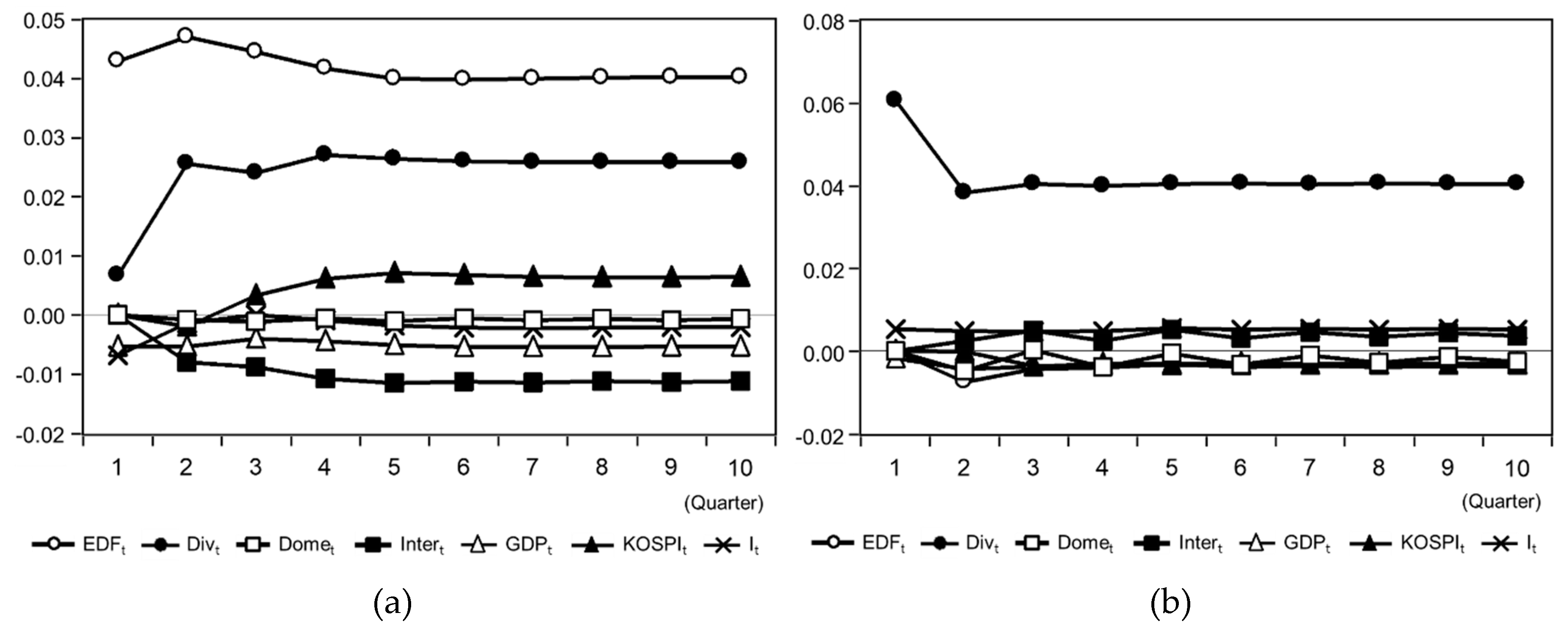
Figure 5.
Cumulative impulse response graph (Group B): (a) cumulative impulse response of EDFt; and (b) cumulative impulse response of Divt.
Figure 5.
Cumulative impulse response graph (Group B): (a) cumulative impulse response of EDFt; and (b) cumulative impulse response of Divt.


Table 1.
Macroeconomic variables of previous studies.
| Studies | Variables | |
|---|---|---|
| Shahandashti et al. (2016) [42] |
|
|
| Vassallo et al. (2012) [43] |
|
|
| Kim et al. (2011) [44] |
|
|
| Jiang et al. (2011) [45] |
|
|
| Chen (2010) [46] |
|
|
| Wong et al. (2010) [47] |
|
|
Table 2.
Variables and descriptions.
| Variables | Descriptions | Period | Frequency |
|---|---|---|---|
| EDFt | Expected Default Frequency | 2001:01–2017:04 | Quarterly |
| Divt | Diversification index | 2001:01–2017:04 | Quarterly |
| Domet | Domestic construction order | 2001:01–2017:04 | Quarterly |
| Intert | International construction order | 2001:01–2017:04 | Quarterly |
| GDPt | Gross Domestic Product | 2001:01–2017:04 | Quarterly |
| KOSPIt | Korea Composite Stock Price Index | 2001:01–2017:04 | Quarterly |
| It | Interest rate | 2001:01–2017:04 | Quarterly |
Table 3.
Tests for unit roots (Augmented Dickey–Fuller tests).
| Variables | Level | 1st Differencing | |||
|---|---|---|---|---|---|
| t-Statistic | p-Value | t-Statistic | p-Value | ||
| Group A (Top 20) | EDFt | −2.288254 | 0.4341 | −5.742322 | 0.0001 |
| Divt | −2.256928 | 0.4509 | −8.428268 | 0.0000 | |
| Domet | −2.176384 | 0.4940 | −10.00393 | 0.0000 | |
| Intert | −2.023805 | 0.5776 | −7.692541 | 0.0000 | |
| GDPt | −2.196584 | 0.4835 | −8.557918 | 0.0000 | |
| KOSPIt | −2.537528 | 0.3098 | −7.670869 | 0.0000 | |
| It | −2.636346 | 0.2662 | −5.970069 | 0.0000 | |
| Group B (Bottom 20) | EDFt | −1.934036 | 0.6257 | −7.074419 | 0.0000 |
| Divt | −1.256623 | 0.8897 | −11.18367 | 0.0000 | |
| Domet | −2.176384 | 0.4940 | −10.00393 | 0.0000 | |
| Intert | −2.023805 | 0.5776 | −7.692541 | 0.0000 | |
| GDPt | −2.196584 | 0.4835 | −8.557918 | 0.0000 | |
| KOSPtt | −2.537528 | 0.3098 | −7.670869 | 0.0000 | |
| It | −2.636346 | 0.2662 | −5.970069 | 0.0000 | |
Note: Paraphrase indicates the signification number of lags chosen based on Schwartz Information Criteria (SIC).
Table 4.
Lag specification results.
| Lag | Group A (Top 20) | Group B (Bottom 20) |
|---|---|---|
| 0 | −4.790108 | −4.644374 |
| 1 | −14.78307 * | −14.08532 * |
| 2 | −12.63590 | −12.16952 |
| 3 | −11.02191 | −10.32565 |
| 4 | −9.906206 | −9.554788 |
| 5 | −10.01882 | −9.074798 |
Note: * Significance at 5% level.
Table 5.
Co-integration Test Results.
| Group | Null Hypothesis | Test Statistic | 0.05 Critical Value | p-Value |
|---|---|---|---|---|
| Group A (Top 20) | r = 0 * | 184.7436 | 134.6780 | 0.0000 |
| r ≤ 1 * | 119.0589 | 103.8473 | 0.0034 | |
| r ≤ 2 | 76.21558 | 76.97277 | 0.0570 | |
| r ≤ 3 | 46.73913 | 54.07904 | 0.1915 | |
| r ≤ 4 | 25.40241 | 35.19275 | 0.3762 | |
| r ≤ 5 | 10.00070 | 20.26184 | 0.6398 | |
| r ≤ 6 | 3.267762 | 9.164546 | 0.5319 | |
| Group B (Bottom 20) | r = 0 * | 187.1327 | 134.6780 | 0.0000 |
| r ≤ 1 * | 120.6725 | 103.8473 | 0.0024 | |
| r ≤ 2 * | 84.07724 | 76.97277 | 0.0130 | |
| r ≤ 3 | 53.04259 | 54.07904 | 0.0617 | |
| r ≤ 4 | 26.41871 | 35.19275 | 0.3190 | |
| r ≤ 5 | 10.00521 | 20.26184 | 0.6393 | |
| r ≤ 6 | 3.727490 | 9.164546 | 0.4542 |
Note: * Significance at 5% level; r is co-integration rank.
Table 6.
Results of Granger causality test—Group A (Top 20).
| Causality | Lag | F-Statistic | p-Value | Causality | Lag | F-Statistic | p-Value | ||||
|---|---|---|---|---|---|---|---|---|---|---|---|
| Divt | → | EDFt | 1 | 0.03897 | 0.8441 | Divt | → | EDFt | 2 | 0.08274 | 0.9207 |
| EDFt | → | Divt | 1 | 0.00630 | 0.9370 | EDFt | → | Divt | 2 | 0.80825 | 0.4504 |
| Domet | → | EDFt | 1 | 1.64984 | 0.2036 | Domet | → | EDFt | 2 | 1.49146 | 0.2331 |
| EDFt | → | Domet | 1 | 1.71782 | 0.1947 | EDFt | → | Domet | 2 | 1.13456 | 0.3283 |
| Intert | → | EDFt | 1 | 2.06555 | 0.1555 | Intert | → | EDFt | 2 | 0.81739 | 0.4464 |
| EDFt | → | Intert | 1 | 1.88974 | 0.1740 | EDFt | → | Intert | 2 | 1.98089 | 0.1467 |
| GDPt | → | EDFt | 1 | 0.98597 | 0.3245 | GDPt | → | EDFt | 2 | 0.33846 | 0.7142 |
| EDFt | → | GDPt | 1 | 0.00267 | 0.9589 | EDFt | → | GDPt | 2 | 0.85788 | 0.4291 |
| KOSPIt | → | EDFt | 1 | 1.74257 | 0.1915 | KOSPIt | → | EDFt | 2 | 0.83698 | 0.4379 |
| EDFt | → | KOSPIt | 1 | 0.01985 | 0.8884 | EDFt | → | KOSPIt | 2 | 1.40062 | 0.2543 |
| It | → | EDFt | 1 | 0.15797 | 0.6924 | It | → | EDFt | 2 | 0.18248 | 0.8337 |
| EDFt | → | It | 1 | 6.00536 | 0.0170 ** | EDFt | → | It | 2 | 4.08024 | 0.0217 ** |
| Domet | → | Divt | 1 | 4.81324 | 0.0319 ** | Domet | → | Divt | 2 | 3.31613 | 0.0429 ** |
| Divt | → | Domet | 1 | 45.49460 | 0.0000 *** | Divt | → | Domet | 2 | 7.38780 | 0.0013 *** |
| Intert | → | Divt | 1 | 0.14785 | 0.7019 | Intert | → | Divt | 2 | 0.82550 | 0.4428 |
| Divt | → | Intert | 1 | 0.33952 | 0.5622 | Divt | → | Intert | 2 | 0.60570 | 0.5489 |
| GDPt | → | Divt | 1 | 1.50307 | 0.2247 | GDPt | → | Divt | 2 | 0.88791 | 0.4168 |
| Divt | → | GDPt | 1 | 0.17637 | 0.6759 | Divt | → | GDPt | 2 | 0.87170 | 0.4234 |
| KOSPIt | → | Divt | 1 | 0.45708 | 0.5014 | KOSPIt | → | Divt | 2 | 0.25796 | 0.7735 |
| Divt | → | KOSPIt | 1 | 0.45731 | 0.5013 | Divt | → | KOSPIt | 2 | 0.31094 | 0.7339 |
| It | → | Divt | 1 | 3.12513 | 0.0819 * | It | → | Divt | 2 | 1.68616 | 0.1937 |
| Divt | → | It | 1 | 0.71606 | 0.4006 | Divt | → | It | 2 | 1.10181 | 0.3388 |
| Intert | → | Domet | 1 | 2.72054 | 0.1040 | Intert | → | Domet | 2 | 0.24470 | 0.7837 |
| Domet | → | Intert | 1 | 0.89698 | 0.3472 | Domet | → | Intert | 2 | 0.04754 | 0.9536 |
| GDPt | → | Domet | 1 | 21.36440 | 0.0000 *** | GDPt | → | Domet | 2 | 1.67801 | 0.1952 |
| Domet | → | GDPt | 1 | 3.31413 | 0.0734 * | Domet | → | GDPt | 2 | 1.97320 | 0.1478 |
| KOSPIt | → | Domet | 1 | 12.95720 | 0.0006 *** | KOSPIt | → | Domet | 2 | 0.36948 | 0.6926 |
| Domet | → | KOSPIt | 1 | 0.60473 | 0.4396 | Domet | → | KOSPIt | 2 | 1.23951 | 0.2967 |
| It | → | Domet | 1 | 19.07310 | 0.0001 *** | It | → | Domet | 2 | 2.08284 | 0.1333 |
| Domet | → | It | 1 | 0.95934 | 0.3310 | Domet | → | It | 2 | 1.05720 | 0.3537 |
| GDPt | → | Intert | 1 | 7.17528 | 0.0094 *** | GDPt | → | Intert | 2 | 0.37230 | 0.6907 |
| Intert | → | GDPt | 1 | 0.59938 | 0.4417 | Intert | → | GDPt | 2 | 0.32007 | 0.7273 |
| KOSPIt | → | Intert | 1 | 27.07080 | 0.0000 *** | KOSPIt | → | Intert | 2 | 3.83421 | 0.0270 ** |
| Intert | → | KOSPIt | 1 | 1.55828 | 0.2165 | Intert | → | KOSPIt | 2 | 2.08853 | 0.1326 |
| It | → | Intert | 1 | 1.09998 | 0.2982 | It | → | Intert | 2 | 0.39386 | 0.6761 |
| Intert | → | It | 1 | 0.02404 | 0.8773 | Intert | → | It | 2 | 1.36581 | 0.2629 |
| KOSPIt | → | GDPt | 1 | 0.72753 | 0.3969 | KOSPIt | → | GDPt | 2 | 6.44671 | 0.0029 *** |
| GDPt | → | KOSPIt | 1 | 3.33492 | 0.0725 * | GDPt | → | KOSPIt | 2 | 3.31223 | 0.0431 ** |
| It | → | GDPt | 1 | 3.88050 | 0.0532 * | It | → | GDPt | 2 | 2.55114 | 0.0863 * |
| GDPt | → | It | 1 | 1.55181 | 0.2174 | GDPt | → | It | 2 | 4.46511 | 0.0155 ** |
| It | → | KOSPIt | 1 | 5.84890 | 0.0184 ** | It | → | KOSPIt | 2 | 4.40046 | 0.0164 ** |
| KOSPIt | → | It | 1 | 0.75323 | 0.3887 | KOSPIt | → | It | 2 | 4.79273 | 0.0117 ** |
Note: *** 1% Significance level; ** 5% Significance level; * 10% Significance level.
Table 7.
Results of Granger causality test—Group B (Bottom 20).
| Causality | Lag | F-Statistic | p-Value | Causality | Lag | F-Statistic | p-Value | ||||
|---|---|---|---|---|---|---|---|---|---|---|---|
| Divt | → | EDFt | 1 | 16.13920 | 0.0002 *** | Divt | → | EDFt | 2 | 9.08397 | 0.0004 *** |
| EDFt | → | Divt | 1 | 0.49876 | 0.4826 | EDFt | → | Divt | 2 | 0.64712 | 0.5271 |
| Domet | → | EDFt | 1 | 0.09912 | 0.7539 | Domet | → | EDFt | 2 | 0.18716 | 0.8298 |
| EDFt | → | Domet | 1 | 33.95010 | 0.0000 *** | EDFt | → | Domet | 2 | 4.27682 | 0.0183 ** |
| Intert | → | EDFt | 1 | 0.07290 | 0.7880 | Intert | → | EDFt | 2 | 0.17063 | 0.8435 |
| EDFt | → | Intert | 1 | 1.94856 | 0.1676 | EDFt | → | Intert | 2 | 3.25771 | 0.0453 ** |
| GDPt | → | EDFt | 1 | 0.67917 | 0.4129 | GDPt | → | EDFt | 2 | 0.50428 | 0.6064 |
| EDFt | → | GDPt | 1 | 0.38621 | 0.5365 | EDFt | → | GDPt | 2 | 0.82186 | 0.4444 |
| KOSPIt | → | EDFt | 1 | 0.00719 | 0.9327 | KOSPIt | → | EDFt | 2 | 0.00421 | 0.9958 |
| EDFt | → | KOSPIt | 1 | 0.33005 | 0.5676 | EDFt | → | KOSPIt | 2 | 1.30267 | 0.2793 |
| It | → | EDFt | 1 | 4.38476 | 0.0402 ** | It | → | EDFt | 2 | 2.19165 | 0.1205 |
| EDFt | → | It | 1 | 1.26409 | 0.2651 | EDFt | → | It | 2 | 0.24124 | 0.7864 |
| Domet | → | Divt | 1 | 0.87802 | 0.3523 | Domet | → | Divt | 2 | 0.31499 | 0.7310 |
| Divt | → | Domet | 1 | 45.31040 | 0.0000 *** | Divt | → | Domet | 2 | 10.76850 | 0.0001 *** |
| Intert | → | Divt | 1 | 0.60425 | 0.4398 | Intert | → | Divt | 2 | 0.37339 | 0.6900 |
| Divt | → | Intert | 1 | 0.10362 | 0.7486 | Divt | → | Intert | 2 | 0.29525 | 0.7454 |
| GDPt | → | Divt | 1 | 2.40636 | 0.1258 | GDPt | → | Divt | 2 | 1.61471 | 0.2073 |
| Divt | → | GDPt | 1 | 0.03293 | 0.8566 | Divt | → | GDPt | 2 | 0.86908 | 0.4245 |
| KOSPIt | → | Divt | 1 | 1.00157 | 0.3207 | KOSPIt | → | Divt | 2 | 0.56680 | 0.5703 |
| Divt | → | KOSPIt | 1 | 1.26919 | 0.2641 | Divt | → | KOSPIt | 2 | 0.73702 | 0.4828 |
| It | → | Divt | 1 | 4.09666 | 0.0471 ** | It | → | Divt | 2 | 1.98378 | 0.1463 |
| Divt | → | It | 1 | 1.43270 | 0.2357 | Divt | → | It | 2 | 1.63926 | 0.2026 |
| Intert | → | Domet | 1 | 2.72054 | 0.1040 | Intert | → | Domet | 2 | 0.24470 | 0.7837 |
| Domet | → | Intert | 1 | 0.89698 | 0.3472 | Domet | → | Intert | 2 | 0.04754 | 0.9536 |
| GDPt | → | Domet | 1 | 21.36440 | 0.0000 *** | GDPt | → | Domet | 2 | 1.67801 | 0.1952 |
| Domet | → | GDPt | 1 | 3.31413 | 0.0734 * | Domet | → | GDPt | 2 | 1.97320 | 0.1478 |
| KOSPIt | → | Domet | 1 | 12.95720 | 0.0006 *** | KOSPIt | → | Domet | 2 | 0.36948 | 0.6926 |
| Domet | → | KOSPIt | 1 | 0.60473 | 0.4396 | Domet | → | KOSPIt | 2 | 1.23951 | 0.2967 |
| It | → | Domet | 1 | 19.07310 | 0.0001 *** | It | → | Domet | 2 | 2.08284 | 0.1333 |
| Domet | → | It | 1 | 0.95934 | 0.3310 | Domet | → | It | 2 | 1.05720 | 0.3537 |
| GDPt | → | Intert | 1 | 7.17528 | 0.0094 *** | GDPt | → | Intert | 2 | 0.37230 | 0.6907 |
| Intert | → | GDPt | 1 | 0.59938 | 0.4417 | Intert | → | GDPt | 2 | 0.32007 | 0.7273 |
| KOSPIt | → | Intert | 1 | 27.07080 | 0.0000 *** | KOSPIt | → | Intert | 2 | 3.83421 | 0.0270 ** |
| Intert | → | KOSPIt | 1 | 1.55828 | 0.2165 | Intert | → | KOSPIt | 2 | 2.08853 | 0.1326 |
| It | → | Intert | 1 | 1.09998 | 0.2982 | It | → | Intert | 2 | 0.39386 | 0.6761 |
| Intert | → | It | 1 | 0.02404 | 0.8773 | Intert | → | It | 2 | 1.36581 | 0.2629 |
| KOSPIt | → | GDPt | 1 | 0.72753 | 0.3969 | KOSPIt | → | GDPt | 2 | 6.44671 | 0.0029 *** |
| GDPt | → | KOSPIt | 1 | 3.33492 | 0.0725 * | GDPt | → | KOSPIt | 2 | 3.31223 | 0.0431 ** |
| It | → | GDPt | 1 | 3.88050 | 0.0532 * | It | → | GDPt | 2 | 2.55114 | 0.0863 * |
| GDPt | → | It | 1 | 1.55181 | 0.2174 | GDPt | → | It | 2 | 4.46511 | 0.0155 ** |
| It | → | KOSPIt | 1 | 5.84890 | 0.0184 ** | It | → | KOSPIt | 2 | 4.40046 | 0.0164 ** |
| KOSPIt | → | It | 1 | 0.75323 | 0.3887 | KOSPIt | → | It | 2 | 4.79273 | 0.0117 ** |
Note: *** 1% Significance level; ** 5% Significance level; * 10% Significance level.
Table 8.
Impulse response results—Group A.
| Dependent Variable | Period (Quarter) | Independent Variables | ||||||
|---|---|---|---|---|---|---|---|---|
| EDFt | Divt | Domet | Intert | GDPt | KOSPIt | It | ||
| EDFt | 1 | 0.04866 | 0.00000 | −0.00946 | 0.00842 | −0.01097 | −0.03156 | −0.00196 |
| 2 | 0.07274 | −0.00088 | −0.00445 | 0.00676 | −0.01468 | −0.03767 | 0.00396 | |
| 3 | 0.08082 | −0.00003 | −0.00794 | 0.00734 | −0.01420 | −0.03276 | 0.00593 | |
| 4 | 0.08368 | 0.00074 | −0.00414 | 0.00784 | −0.01588 | −0.02893 | 0.00613 | |
| 5 | 0.08272 | 0.00087 | −0.00692 | 0.00705 | −0.01596 | −0.02775 | 0.00550 | |
| 6 | 0.08283 | 0.00112 | −0.00485 | 0.00816 | −0.01641 | −0.02850 | 0.00548 | |
| 7 | 0.08233 | 0.00074 | −0.00662 | 0.00716 | −0.01613 | −0.02871 | 0.00536 | |
| 8 | 0.08276 | 0.00098 | −0.00522 | 0.00804 | −0.01624 | −0.02896 | 0.00554 | |
| 9 | 0.08253 | 0.00075 | −0.00633 | 0.00726 | −0.01611 | −0.02874 | 0.00545 | |
| 10 | 0.08276 | 0.00097 | −0.00543 | 0.00791 | −0.01621 | −0.02881 | 0.00554 | |
| Divt | 1 | 0.00818 | 0.03395 | 0.00800 | 0.00042 | −0.00458 | 0.00374 | −0.00414 |
| 2 | 0.01270 | 0.03319 | 0.00289 | −0.00408 | −0.00731 | 0.00300 | −0.00355 | |
| 3 | 0.01514 | 0.03405 | 0.00602 | 0.00043 | −0.00749 | 0.00096 | −0.00284 | |
| 4 | 0.01524 | 0.03295 | 0.00352 | −0.00276 | −0.00744 | 0.00156 | −0.00288 | |
| 5 | 0.01609 | 0.03381 | 0.00567 | −0.00055 | −0.00752 | 0.00168 | −0.00256 | |
| 6 | 0.01565 | 0.03330 | 0.00400 | −0.00218 | −0.00751 | 0.00216 | −0.00279 | |
| 7 | 0.01595 | 0.03372 | 0.00534 | −0.00094 | −0.00761 | 0.00193 | −0.00268 | |
| 8 | 0.01564 | 0.03339 | 0.00424 | −0.00188 | −0.00754 | 0.00204 | −0.00280 | |
| 9 | 0.01587 | 0.03363 | 0.00512 | −0.00115 | −0.00760 | 0.00189 | −0.00270 | |
| 10 | 0.01570 | 0.03344 | 0.00442 | −0.00172 | −0.00754 | 0.00200 | −0.00277 | |
Table 9.
Cumulative impulse response results—Group A.
| Dependent Variable | Period (Quarter) | Independent Variables | ||||||
|---|---|---|---|---|---|---|---|---|
| EDFt | Divt | Domet | Intert | GDPt | KOSPIt | It | ||
| EDFt | 1 | 0.04866 | 0.00000 | −0.00946 | 0.00842 | −0.01097 | −0.03156 | −0.00196 |
| 2 | 0.12140 | −0.00088 | −0.01391 | 0.01518 | −0.02564 | −0.06923 | 0.00201 | |
| 3 | 0.20222 | −0.00091 | −0.02185 | 0.02252 | −0.03984 | −0.10199 | 0.00793 | |
| 4 | 0.28590 | −0.00016 | −0.02599 | 0.03037 | −0.05572 | −0.13091 | 0.01406 | |
| 5 | 0.36861 | 0.00072 | −0.03291 | 0.03741 | −0.07167 | −0.15866 | 0.01956 | |
| 6 | 0.45144 | 0.00183 | −0.03776 | 0.04557 | −0.08808 | −0.18716 | 0.02505 | |
| 7 | 0.53376 | 0.00257 | −0.04439 | 0.05273 | −0.10421 | −0.21587 | 0.03040 | |
| 8 | 0.61652 | 0.00355 | −0.04961 | 0.06076 | −0.12044 | −0.24483 | 0.03594 | |
| 9 | 0.69905 | 0.00430 | −0.05594 | 0.06803 | −0.13656 | −0.27357 | 0.04140 | |
| 10 | 0.78181 | 0.00527 | −0.06137 | 0.07593 | −0.15276 | −0.30238 | 0.04693 | |
| Divt | 1 | 0.00818 | 0.03395 | 0.00800 | 0.00042 | −0.00458 | 0.00374 | −0.00414 |
| 2 | 0.02088 | 0.06713 | 0.01089 | −0.00366 | −0.01189 | 0.00674 | −0.00769 | |
| 3 | 0.03602 | 0.10118 | 0.01691 | −0.00323 | −0.01938 | 0.00770 | −0.01053 | |
| 4 | 0.05125 | 0.13413 | 0.02043 | −0.00599 | −0.02683 | 0.00927 | −0.01341 | |
| 5 | 0.06735 | 0.16794 | 0.02610 | −0.00654 | −0.03434 | 0.01094 | −0.01597 | |
| 6 | 0.08300 | 0.20124 | 0.03010 | −0.00871 | −0.04186 | 0.01310 | −0.01876 | |
| 7 | 0.09894 | 0.23496 | 0.03544 | −0.00965 | −0.04947 | 0.01503 | −0.02144 | |
| 8 | 0.11458 | 0.26835 | 0.03968 | −0.01153 | −0.05701 | 0.01707 | −0.02423 | |
| 9 | 0.13045 | 0.30199 | 0.04480 | −0.01268 | −0.06460 | 0.01896 | −0.02693 | |
| 10 | 0.14614 | 0.33543 | 0.04922 | −0.01440 | −0.07214 | 0.02096 | −0.02970 | |
Table 10.
Impulse response results—Group B.
| Dependent Variable | Period (Quarter) | Independent Variables | ||||||
|---|---|---|---|---|---|---|---|---|
| EDFt | Divt | Domet | Intert | GDPt | KOSPIt | It | ||
| EDFt | 1 | 0.04300 | 0.00667 | 0.00000 | 0.00000 | −0.00534 | 0.00000 | −0.00678 |
| 2 | 0.04712 | 0.02561 | −0.00081 | −0.00796 | −0.00534 | −0.00195 | −0.00138 | |
| 3 | 0.04451 | 0.02404 | −0.00110 | −0.00875 | −0.00401 | 0.00334 | 0.00004 | |
| 4 | 0.04171 | 0.02709 | −0.00051 | −0.01078 | −0.00439 | 0.00610 | −0.00086 | |
| 5 | 0.04001 | 0.02640 | −0.00100 | −0.01147 | −0.00508 | 0.00707 | −0.00177 | |
| 6 | 0.03984 | 0.02606 | −0.00053 | −0.01128 | −0.00542 | 0.00675 | −0.00212 | |
| 7 | 0.03999 | 0.02582 | −0.00088 | −0.01144 | −0.00541 | 0.00648 | −0.00218 | |
| 8 | 0.04021 | 0.02582 | −0.00059 | −0.01117 | −0.00539 | 0.00638 | −0.00207 | |
| 9 | 0.04021 | 0.02587 | −0.00084 | −0.01132 | −0.00533 | 0.00638 | −0.00207 | |
| 10 | 0.04024 | 0.02588 | −0.00064 | −0.01120 | −0.00535 | 0.00640 | −0.00203 | |
| Divt | 1 | 0.00000 | 0.06065 | 0.00000 | 0.00000 | −0.00170 | 0.00000 | 0.00533 |
| 2 | −0.00743 | 0.03835 | −0.00482 | 0.00248 | −0.00427 | −0.00010 | 0.00486 | |
| 3 | −0.00428 | 0.04044 | 0.00032 | 0.00496 | −0.00369 | −0.00364 | 0.00472 | |
| 4 | −0.00398 | 0.03999 | −0.00384 | 0.00251 | −0.00305 | −0.00338 | 0.00489 | |
| 5 | −0.00318 | 0.04042 | −0.00054 | 0.00517 | −0.00319 | −0.00340 | 0.00551 | |
| 6 | −0.00380 | 0.04055 | −0.00326 | 0.00311 | −0.00295 | −0.00336 | 0.00516 | |
| 7 | −0.00347 | 0.04039 | −0.00104 | 0.00464 | −0.00316 | −0.00324 | 0.00546 | |
| 8 | −0.00379 | 0.04054 | −0.00284 | 0.00343 | −0.00299 | −0.00329 | 0.00517 | |
| 9 | −0.00356 | 0.04041 | −0.00137 | 0.00437 | −0.00315 | −0.00325 | 0.00539 | |
| 10 | −0.00373 | 0.04050 | −0.00257 | 0.00366 | −0.00302 | −0.00329 | 0.00520 | |
Table 11.
Cumulative impulse response results—Group B.
| Dependent Variable | Period (Quarter) | Independent Variables | ||||||
|---|---|---|---|---|---|---|---|---|
| EDFt | Divt | Domet | Intert | GDPt | KOSPIt | It | ||
| EDFt | 1 | 0.04300 | 0.00667 | 0.00000 | 0.00000 | −0.00534 | 0.00000 | −0.00676 |
| 2 | 0.09012 | 0.03227 | −0.00081 | −0.00796 | −0.01068 | −0.00195 | −0.00814 | |
| 3 | 0.13464 | 0.05632 | −0.00190 | −0.01671 | −0.01469 | 0.00139 | −0.00810 | |
| 4 | 0.17634 | 0.08340 | −0.00241 | −0.02749 | −0.01908 | 0.00749 | −0.00896 | |
| 5 | 0.21636 | 0.10980 | −0.00342 | −0.03896 | −0.02415 | 0.01456 | −0.01073 | |
| 6 | 0.25620 | 0.13586 | −0.00395 | −0.05024 | −0.02958 | 0.02131 | −0.01284 | |
| 7 | 0.29619 | 0.16168 | −0.00483 | −0.06168 | −0.03499 | 0.02779 | −0.01502 | |
| 8 | 0.33640 | 0.18750 | −0.00542 | −0.07285 | −0.04037 | 0.03417 | −0.01710 | |
| 9 | 0.37661 | 0.21337 | −0.00625 | −0.08417 | −0.04571 | 0.04054 | −0.01916 | |
| 10 | 0.41685 | 0.23925 | −0.00689 | −0.09537 | −0.05106 | 0.04695 | −0.02119 | |
| Divt | 1 | 0.00000 | 0.06065 | 0.00000 | 0.00000 | −0.00170 | 0.00000 | 0.00533 |
| 2 | −0.00743 | 0.09900 | −0.00482 | 0.00248 | −0.00596 | −0.00010 | 0.01018 | |
| 3 | −0.01171 | 0.13944 | −0.00450 | 0.00743 | −0.00966 | −0.00374 | 0.01490 | |
| 4 | −0.01570 | 0.17943 | −0.00834 | 0.00994 | −0.01271 | −0.00711 | 0.01979 | |
| 5 | −0.01888 | 0.21984 | −0.00889 | 0.01512 | −0.01590 | −0.01051 | 0.02530 | |
| 6 | −0.02268 | 0.26039 | −0.01214 | 0.01822 | −0.01884 | −0.01387 | 0.03046 | |
| 7 | −0.02614 | 0.30078 | −0.01318 | 0.02286 | −0.02200 | −0.01711 | 0.03591 | |
| 8 | −0.02993 | 0.34132 | −0.01602 | 0.02629 | −0.02499 | −0.02040 | 0.04108 | |
| 9 | −0.03349 | 0.38172 | −0.01740 | 0.03066 | −0.02815 | −0.02364 | 0.04647 | |
| 10 | −0.03722 | 0.42222 | −0.01997 | 0.03429 | −0.03117 | −0.02694 | 0.05167 | |
© 2019 by the authors. Licensee MDPI, Basel, Switzerland. This article is an open access article distributed under the terms and conditions of the Creative Commons Attribution (CC BY) license (http://creativecommons.org/licenses/by/4.0/).
Share and Cite
MDPI and ACS Style
Han, M.; Lee, S.; Kim, J. Effectiveness of Diversification Strategies for Ensuring Financial Sustainability of Construction Companies in the Republic of Korea. Sustainability 2019, 11, 3076. https://doi.org/10.3390/su11113076
AMA Style
Han M, Lee S, Kim J. Effectiveness of Diversification Strategies for Ensuring Financial Sustainability of Construction Companies in the Republic of Korea. Sustainability. 2019; 11(11):3076. https://doi.org/10.3390/su11113076
Chicago/Turabian StyleHan, Manchun, Sanghyo Lee, and Jaejun Kim. 2019. "Effectiveness of Diversification Strategies for Ensuring Financial Sustainability of Construction Companies in the Republic of Korea" Sustainability 11, no. 11: 3076. https://doi.org/10.3390/su11113076
Note that from the first issue of 2016, this journal uses article numbers instead of page numbers. See further details here.