Consumption-Based Accounting and the Trade-Carbon Emissions Nexus in Asia: A Heterogeneous, Common Factor Panel Analysis


Energy Studies Institute, National University Singapore, Singapore 119620, Singapore
Sustainability 2018, 10(10), 3627; https://doi.org/10.3390/su10103627
Submission received: 20 July 2018
/
Revised: 24 August 2018
/
Accepted: 3 October 2018
/
Published: 11 October 2018
(This article belongs to the Special Issue Climate Change and Sustainable Development Policy)
Abstract
:This paper considers a recently developed consumption-based carbon emissions database from which emissions calculations are made based on the domestic use of fossil fuels plus the embodied emissions from imports minus exports, to test directly for the importance of trade in national emissions. The People’s Republic of China (PRC) alone is responsible for over half the global outflows of carbon via trade. The econometric estimations—which focused on a panel of 20 Asian countries—determined that: (i) trade flows were significant for consumption-based emissions but not for territory-based emissions; and (ii) exports and imports offset each other in that exports lower consumption-based emissions, whereas imports increase them. Hence, all countries should have both an interest and a responsibility to help lower the carbon intensity of energy in countries that are particularly important for global carbon transfers—the PRC and India.
1. Introduction
Recently, a consumption-based carbon emissions database has been developed [1] from which emissions calculations are made based on the domestic use of fossil fuels plus the embodied emissions from imports minus exports. There has long been a concern that countries—particularly wealthy ones—might lower emissions via international trade in such a way that those emissions reductions are (at least) offset by increases elsewhere—i.e., in the territory(ies) where the traded goods/services originate (e.g., [2]). Yet, despite that concern and the availability of data that allows researchers to test directly for the importance of trade in national emissions, most economic-based inquiries into the trade-emissions relationship still employ conventionally-measured territory-based carbon data (e.g., [3]).
This paper compares and analyzes both consumption-based and territory-based carbon emissions data to estimate relationships among emissions, trade flows, income, energy structure, and economic structure/energy intensity. We focus on 20 Asian countries/economies for which data could be assembled (Those countries/economies (and their World Bank code) are: Bangladesh (BGD); Cambodia (KHM); the People’s Republic of China (CHN/PRC); Hong Kong, China (HKG); India (IND); Indonesia (IDN); Japan (JPN); Kazakhstan (KAZ); Kyrgyz Republic (KGZ); Malaysia (MYS); Mongolia (MNG); Nepal (NPL); Pakistan (PAK); Philippines (PHL); Singapore (SGP); Republic of Korea (KOR); Sri Lanka (LKA); Taipei, China (TWN); Thailand (THA); and Viet Nam (VNM)). Not only does this group include many of the world’s most rapidly growing economies, these 20 countries/economies account for over half of the world’s population and nearly half (45%) of all territory-based carbon emissions.
Whether the global trade system would facilitate the re-location of pollution-intensive industries to countries with less concern for environmental quality has been a popular topic in environmental economics. The literature has developed in two somewhat distinct strands: Mostly theoretical models and mostly empirical analyses. The theoretical literature has tended to support a finding of the migration of polluting industries (either through trade or capital flight) from a country that has introduced a pollution policy (e.g., References [4,5,6]). By contrast, the empirical literature produced more ambiguous results. For example, References [7,8,9,10] rejected the so-called “pollution haven” hypothesis, by finding that factor endowments were more important than pollution tolerance in determining trade patterns and plant location decisions. Meanwhile, References [11,12,13,14,15] determined that openness to trade in developing countries led to specialization or an increase in pollution-intensive production there. The recent literature review in Reference [3] suggests that the ambiguity among the empirical studies remains. Yet, as mentioned above, the recent development of a consumption-based carbon emissions dataset creates the potential to substantially advance the trade-emissions literature.
Some studies that have employed both consumption-based data and regression analysis have not, however, considered trade variables as drivers of those consumption-based emissions (e.g., References [16,17]). Again, the recent trade-focused, environmental economics literature has maintained the use of the territory-based emissions data only (e.g., References [3,18]).
The only papers we know of that have (i) compared estimations made with consumption-based emissions to estimations made with territorial-based emissions and (ii) considered trade variables are References [19,20,21,22,23]. Knight and Schor [19] analyzed high income countries only and did so by considering a short-run model (i.e., the data were first-differenced after converting to natural logarithms), and Reference [20] was purely cross-sectional (only data from 2008 was used) and did not consider imports (only exports/GDP was analyzed). Fernandez-Amador et al. [21] used a panel-based dataset (observations from five intermittent years), and they did not estimate separate effects for imports and exports (rather, they considered trade openness only). Hasanov et al. [23] focused on nine oil exporting counties. Liddle [22] employed the same methods as used here and analyzed a global dataset. The present paper is different from Reference [22]—and the other four papers mentioned above—in that it (i) focuses on Asian countries and (ii) considers a more structurally-based model. What is important is that all five of the published papers—as well as the present one—found an insignificant (to mostly insignificant for the case of Reference [23]) impact of trade on territorial-based carbon emissions; and the three papers (References [19,22,23])—as well as the present one—that considered imports and exports separately found significant, offsetting impacts on consumption-based emissions.
2. Data, Model, and Methods
2.1. Initial Look at Carbon Emissions and Trade both Globally and in Asia
Consumption-based carbon emissions in million tonnes of carbon per year cover 117 countries over 1990–2013 and are updated from [1] (That data is accessed via: http://www.globalcarbonproject.org/carbonbudget/16/data.htm). Consumption-based carbon emissions data can be compared to territory-based carbon emissions (also in million tonnes of carbon per year and for the same countries and time-frame) from [24,25], and a new series can be created: the ratio of consumption-based to territory-based emissions.
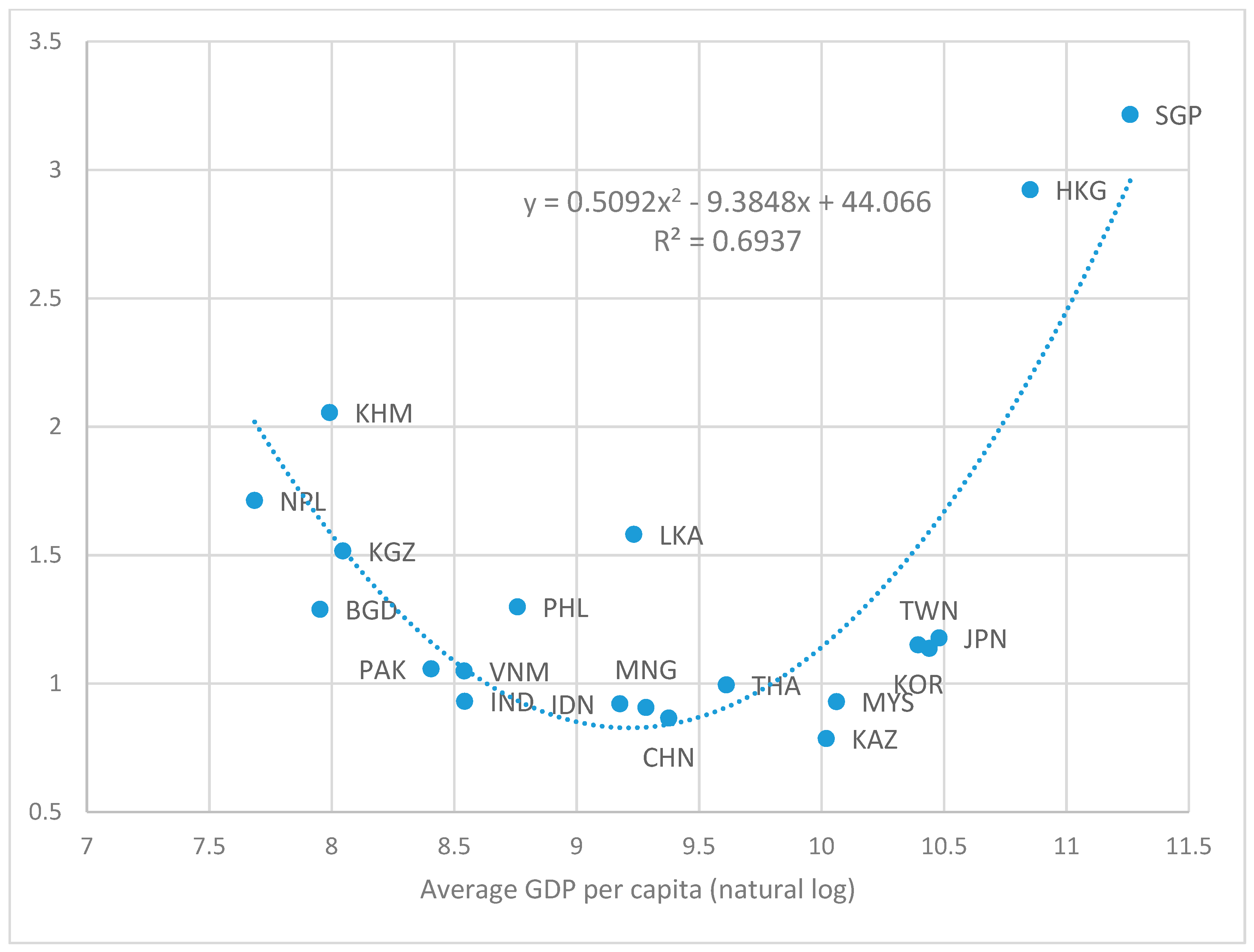
If the consumption-to-territory emissions ratio is greater than one, then a country effectively imports carbon emissions. Of the 117 countries in the global dataset, only 28 countries had a mean ratio (over 1990–2013) of less than one [22]. The average country mean ratio was 1.26, and the mean ratio for each year ranged from 1.2–1.4 [22]. For most countries, the annual ratio was stable: Most countries’ maximum and minimum yearly ratio was within 20–30% of their mean ratio [22]. For the 20 countries/economies considered here, only six had ratios of less than one (see Figure 1). As such, the vast majority of those countries consume more carbon emissions than they produce/emit at home, and the “average” country consumes about one-quarter more carbon emissions than it produces/directly emits.
Figure 1 displays the mean consumption-to-territory emissions ratio plotted against the mean GDP per capita (in log form). The relationship displays a U-shape: Some of the poorest countries (Bangladesh, Cambodia, Kyrgyz Republic, and Nepal) and the wealthy cities (Hong Kong, China; and Singapore) have among the largest ratios; whereas, the countries with ratios near one tend to be middle-income.
The consumption-based and territory-based emissions series can be used to create another new variable, viz., the difference between territory-based and consumption-based emissions, or the net emissions flow; when that net emissions flow is calculated for each country, the importance to world carbon emissions flows of admitting the People’s Republic of China (PRC) into the World Trade Organization (WTO) (the PRC became a member of the WTO on 11 December 2001) becomes evident.
Indeed, since 2005, the PRC has been responsible for over half of global net carbon emissions transfers [22]. Further, the PRC and three other countries—Russia, India, and Kazakhstan—have been responsible for 50–80% of yearly net carbon outflows over 1990–2013, as displayed in Figure 2. The importance of the PRC and India (which surpassed Russia as the second largest source of net emissions flows) for global carbon transfers reflects a combination of (i) the scale of their economies and (ii) the carbon intensity of their energy systems, rather than trade or industry share of GDP. For example, over 2002–2013, exports made up less than 30% of the PRC’s GDP on average, and industry made up a relatively small share of GDP in India (about one-quarter). Moreover, according to data from [1], of the top 10 economic sectors in terms of average yearly carbon flows over 1990–2008 for PRC, only four sectors are classified as energy-intensive, and those four sectors account for less than 40% of the PRC’s average yearly net carbon flows.
Energy systems in Asia tend to be carbon intensive. Indeed, of the 20 countries/economies considered here, fossil fuels average over 80% of energy consumption for eight of them, and for only three (Cambodia, Nepal, and Sri Lanka) do fossil fuels account for less than half of energy consumed. Manufacturing dominates exports in the region and accounts for less than 60% of exports for only four countries (Indonesia, Kazakhstan, Kyrgyz Republic, and Mongolia). Also, the region tends to specialize in exporting that manufacturing to high-income countries. Of the 15 countries considered here that are not high-income themselves, merchandise exports to high-income countries account for less than 55% of all merchandise exports for only Mongolia and Nepal (a majority of whose exports stay in South Asia).
2.2. Model
We start with a Kaya-type identity [26], but divide by population; hence territory-based carbon emissions per capita (CO2T/N) would be:
In other words, CO2T/N equals the product sum of GDP per capita, energy intensity of GDP, and the carbon intensity of energy. Next, we approximate the carbon intensity of energy with the share of energy from fossil fuels (for which data are easier to assemble), shEff, and assume that from now on the nomenclature CO2 refers to per capita emissions. Also, to avoid regressing an identity and following [27], we replace the energy intensity of GDP with industry energy intensity, , and take logs; thus, we have:
Consumption-based emissions are territory-based emissions plus the emissions embodied in imports (COI2) minus the emissions embodied in exports (COX2):
where
In other words, the left-hand-side of Equation (4) equals the import share of GDP times the carbon intensity of imports () divided by the carbon intensity of GDP (). Since the same is true for , Equation (3) becomes:
Since none of the Asian countries have previously priced or currently price carbon, we assume that the ratio of the carbon intensity of exports to the carbon intensity of GDP is unity (i.e., carbon is not a motivation for trade). Similarly, for the same reason (i.e., carbon is not a motivation for any country to export) and for lack of data availability, we assume that the ratio of the carbon intensity of imports to the carbon intensity of GDP is unity, too. Further, when we take logs and substitute for territory-based emissions, we get:
2.3. Additional Data Considered
Other variables, besides carbon emissions, that are included and sourced from the World Bank’s World Development Indicators are: Real GDP per capita (adjusted for PPP and in 2011 international USD); population (to convert emissions to per capita); fossil fuel energy consumption as a share of total energy consumption; industry value added as a share of GDP (to derive industry output); and exports of goods and services and imports of goods and services, both as a percent of GDP (For Taipei, China, the data comes from the International Energy Agency and, for exports and imports, from its national statistical bureau, eng.stat.gov.tw (accessed on 22 May 2017)). Additionally, industry energy consumption—used to calculate industry energy intensity—is sourced from the International Energy Agency. Ultimately, a highly balanced panel of 20 cross-sections and spanning 1990–2013 is created. Summary statistics are displayed in Table 1.
For the macro-level variables we consider, cross-sectional correlation/dependence is expected because of, for example, regional and macroeconomic linkages that manifest themselves through (i) common global shocks; (ii) institutional memberships like Asia Pacific Economic Cooperation (APEC), Association of South-East Asian Nations (ASEAN), and WTO; or (iii) local spillover effects between countries or regions. The variables analyzed are also highly trending, stock-based variables, and thus, may be nonstationary—in other words, their mean, variance, and/or covariance with other variables changes over time. Hence, we expect the data to exhibit both cross-sectional correlation and nonstationarity.
The Pesaran [28] cross-sectional dependence (CD) test (This test is implemented via the STATA command xtcd, which was developed by Markus Eberhardt), which employs the correlation coefficients between the time-series for each panel member, rejected the null hypothesis of cross-sectional independence for each variable considered. Furthermore, the absolute value mean correlation coefficients ranged from 0.4–0.9 (Table 2). The Pesaran [29] panel unit root test for heterogeneous panels allows for cross-sectional dependence to be caused by a single (unobserved) common factor (This test is implemented via the STATA command pescadf, which was developed by Piotr Lewandowski). Lags of the dependent variable are used to control for serial correlation. The test models include individual constants and time trends. The results of that test—shown in Table 3—suggest that (at least most of) the variables are nonstationary in levels.
2.4. Methods
When the errors of panel regressions are cross-sectionally correlated, standard estimation methods can produce inconsistent parameter estimates and incorrect inferences [30]. Also, when ordinary least squares (OLS) regressions are performed on time-series (or on time-series cross-sectional) variables that are not stationary, then measures like R-squared and t-statistics are unreliable, and there is a serious risk of the estimated relationships being spurious [31,32]. Lastly, we think it is likely that the relationships will not be the same for each country—i.e., there should be a substantial degree of heterogeneity.
Given that the data exhibit both cross-sectional correlation and nonstationarity, and likely heterogeneity, we employ a heterogeneous panel estimator that addresses both nonstationarity and cross-sectional dependence, i.e., the Pesaran [33] common correlated effects mean group estimator (CCE-MG) (This estimator is implemented via the STATA command suite xtmg, which was developed by Markus Eberhardt). The CCE-MG estimator accounts for the presence of unobserved common factors by including in the regression cross-sectional averages of the dependent and independent variables, and it is robust to nonstationarity, cointegration, breaks, and serial correlation. Also, as a mean group estimator, CCE-MG first estimates cross-sectional specific regressions and then averages those estimated cross-sectional coefficients to arrive at panel coefficients (standard errors are constructed nonparametrically as described in Reference [34]). Lastly, as diagnostics, we run on the regression residuals and report the results of the Pesaran CD test to determine cross-sectional dependence and the Pesaran CIPS panel unit root test to confirm stationarity.
The purpose of Equations (1)–(6) was to justify the terms to be considered in the regression models and to generate a priori beliefs regarding the signs/significance of the coefficients (we do not want to run a regression on an identity). Hence for the purpose of the regressions, we simplify the last term in parentheses in Equation (6) to be the natural log of import’s share of GDP minus the natural log of export’s share of GDP. Then, the equation to be estimated is:
where subscripts it denote the ith cross-section and tth time period, α is a cross-sectional specific constant, the βs are cross-sectional specific coefficients to be estimated, Z represents the cross-sectional average terms, and ε is the error term. Those cross-sectional average terms are displayed in Equation (8) below:
Like time dummies, the cross-sectional average terms can account for so-called strong-form cross-sectional dependence, i.e., temporary, global shocks. For example, the cross-sectional average time series of GDP will dip/level, corresponding to events like the Asian financial crisis and the Great Recession. But cross-sectional dependence also is caused by so-called spillover effects or weak-form dependence (e.g., international trade), which is much more accurately modeled by cross-sectional averages than merely time dummies/trends.
While, from Equation (2), we do not expect trade shares to impact territory-based carbon emissions, we estimate Equation (7) for both territory-based and consumption-based aggregations of carbon emissions. We do this to test for trade’s effect since some previous territory-based carbon analyses have found such an effect (e.g., References [3,18]). Again, we expect that exports should lower consumption-based emissions; whereas, imports should increase them.
3. Results and Discussion
Table 4 reports the regression results for both territory-based and consumption-based aggregations of emissions. The elasticities for income (GDP per capita) are significant, positive, and highly similar for both territory-based and consumption-based emissions. Likewise for the fossil fuel share of energy, both elasticities are significant, positive, and highly similar. While the mean coefficient is higher for territory-based emissions than for consumption-based, the estimated elasticities are not significantly different at the 95% level (consider the two sets of confidence intervals that are shown in brackets). The elasticity for industrial energy intensity is significant and positive (as expected) for territory-based emissions, but is insignificant for consumption-based emissions. Perhaps this insignificant result for consumption-based emissions reflects that trade among Asian countries is not focused on particularly energy intensive goods.
Importantly, exports and imports share are insignificant for territory-based emissions and significant and offsetting—exports having a negative elasticity, with imports having a positive one—for consumption-based emissions. Again, this was our expected result and is in concert with the findings of References [19,22,23]. While the consumption-based emissions coefficient for exports is larger (in absolute terms) than the same coefficient for imports, the corresponding 95% confidence intervals overlap, and the p-value—for the test on whether their difference (−0.09) was statistically significant—was 0.48.
This insignificant result here for territory-based emissions runs counter, however, to much of the previous trade-carbon emissions literature that has often determined a trade effect despite relying only on territory-based emissions accounting (e.g., Reference [3]). One explanation for the different results for trade variables when territory-based carbon emissions were the dependent variable is the inclusion of the fossil fuel share of energy among the independent variables. Lastly, the CD test statistic (and corresponding high p-values) demonstrate that including cross-sectional averages of the regressors has addressed cross-sectional dependence, since for neither of the regressions can the null hypothesis of cross-sectional independence be rejected.
Because of the importance of the PRC in trade-based carbon flows (e.g., Figure 2), the regressions were run excluding this country. The results were not materially different (results not shown, but available from the author). Also, the time dimension of the panel was split into two segments at 2002—approximately the year of the PRC’s admission into the WTO, and a pooled version of the CCE estimator was used. Those results did not suggest that a different model was valid/necessary over the two regimes—1990–2001 versus 2002–2013 (again, results not shown, but available from the author). A pooled CCE estimator was applied to the full (1990–2013) panel, too. There were some differences between those pooled results and the mean group ones (displayed in Table 4). Of course, the fact that the mean group estimations do differ some from the pooled ones (both when the PRC is included/excluded from the panel) is often interpreted as demonstrating the importance of accounting for heterogeneity.
A common line of inquiry in environmental economics/social science is whether pollution varies nonlinearly with GDP per capita (indeed, there is often overlap between the environment-trade literature and the environment-pollution/environmental Kuznets curve literature). Such nonlinearities are often investigated by estimating emissions as a quadratic (or higher) function of GDP per capita (e.g., Reference [3]). However, it is incorrect to make a nonlinear transformation of a nonstationary (and potentially cointegrated) variable, like GDP per capita, in ordinary least squares [35]. Furthermore, this polynomial model has been criticized for lacking flexibility (e.g., Reference [36]).
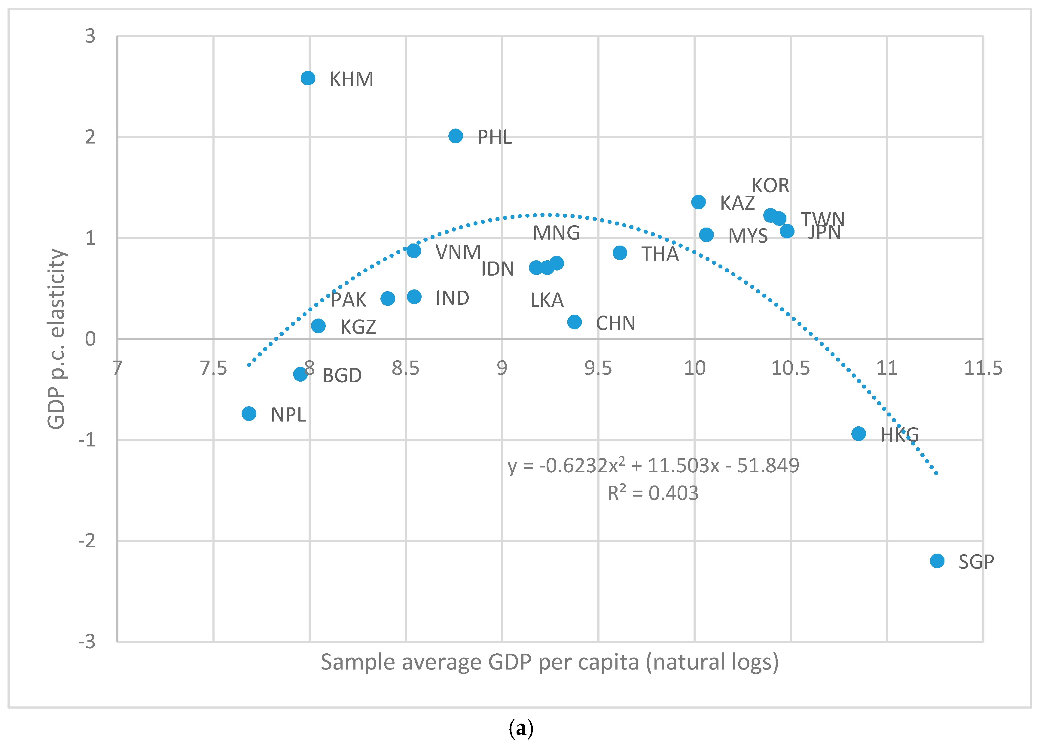
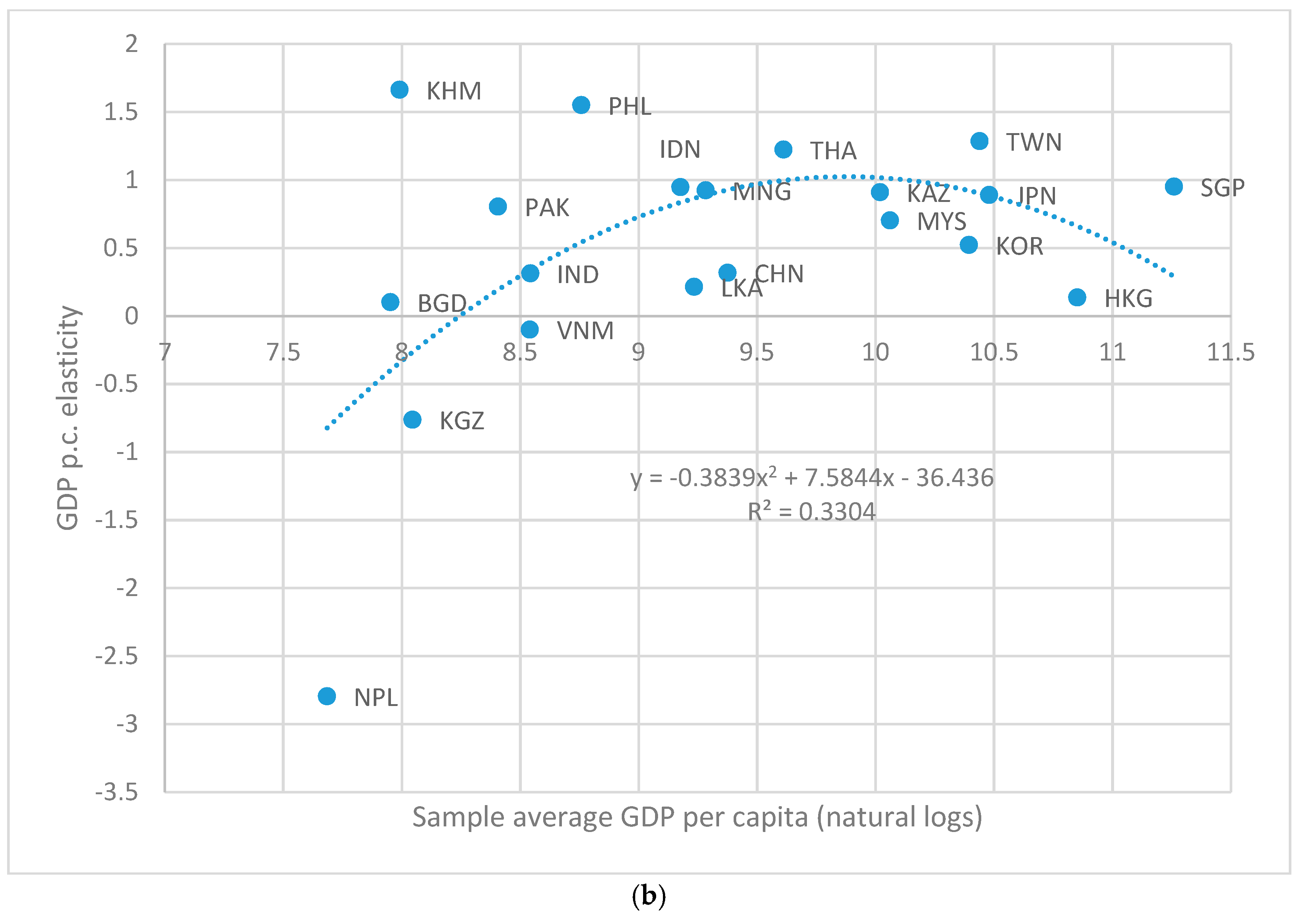
One alternative to the GDP polynomial that takes advantage of the heterogeneous nature of the elasticity estimations (i.e., elasticities are estimated for each cross-section) is to plot individual country-specific GDP per capita elasticity estimates against the individual country average GDP per capita for the whole sample period (as in Reference [27]). Those plots are displayed in Figure 3a,b (Figure 3a (top) for territory-based emissions and Figure 3b (bottom) for consumption-based emissions).
The figures appear to lend credence to the idea that the income elasticity of carbon emissions increases and then falls as income rises since inverted-U polynomial trend lines can be fitted with reasonable accompanying R-squareds. However, focusing on Figure 3a (territory-based emissions), if we assume that Hong Kong, China and Singapore are outliers—because of, for example, their city-state status or because their estimated (negative) elasticities were not statistically significant—the fitted trend line becomes monotonic (albeit with a smaller R-squared). Furthermore, on closer inspection of Figure 3b (consumption-based emissions), the relationship may be better described as a saturation one, i.e., the income elasticity of carbon emissions stops increasing at high levels of income (rather than becoming negative) since the only negative elasticity observations are associated with the lowest income levels. Indeed, a third-order polynomial—in which the income elasticity never dips below the x-axis—fits similarly well as the second-order one (judging by R-squared).
Comparing the individual elasticity estimates (e.g., Figure 3a vs. Figure 3b), most countries have similar estimates for territory-based emissions and consumption-based emissions. However, this is not the case for Hong Kong, China and Singapore. For those two city-states, their income elasticities are negative for territory-based emissions but positive for consumption-based emissions, therefore, providing an example of how one can develop a completely different picture of the income-emissions relationship depending on how those emissions are calculated.
4. Conclusions and Implications
This paper exploited a recently developed consumption-based carbon emissions database (by Reference [1]) from which emissions calculations are made based on the domestic use of fossil fuels plus the embodied emissions from imports minus exports to test directly for the importance of trade in national emissions. Comparing territory-based emissions data to the consumption-based emissions data revealed that most countries are net importers of carbon emissions—their consumption-based emissions are higher than their territory-based emissions. While low and high income countries tend to have the largest ratios of consumption-based emissions to territory-based emissions (e.g., see Figure 1), the several middle-income countries in our Asian panel have ratios greater than one as well.
This study focused on 20 Asian countries/economies—a group that includes many of the world’s most rapidly growing economies, and that together accounts for over half of the world’s population and nearly half of all territory-based carbon emissions (in 2013). Asian countries/economies are an important focus group for carbon emissions and trade because both (i) the energy systems in Asia tend to be carbon intensive, and (ii) the region tends to specialize in exporting its manufacturing to high-income countries. Indeed, the PRC and India are the two largest sources of net (i.e., adjusted for trade) carbon emission flows, and the PRC is responsible for over half of such global net carbon emissions transfers.
The econometric estimations showed that: (i) trade flows (imports and exports) mattered for consumption-based emissions but not for territory-based emissions; and (ii) exports and imports offset each other in that exports lower consumption-based emissions, whereas imports increase them. Those results were both credible/easily justified (e.g., Equations (2)–(6)), and in concert with the three previous analyses that compared trade-carbon models using those two different aggregations of emissions as dependent variables and considered imports and exports (separately) as independent variables ([19,22,23]). In sum, for territory-based emissions, fossil fuel consumption (but not trade) matters; and for consumption-based emissions, trade patterns (exports, imports) matter, and trading partners’ fossil fuel consumption matter [22] (In contrast to Reference [22] analyzing a global dataset, this analysis focusing on Asia did not find that fossil fuel content of a country’s energy mix was significantly more important for territory-based emissions than for consumption-based emissions. Perhaps this failure reflects the previously discussed relative fossil fuel intensity of all Asian countries’ energy systems). Therefore, for modelers wanting to investigate further trade’s role in carbon emissions, it is important both (i) to consider consumption-based emissions and (ii) to consider imports and exports separately.
Given that (i) global carbon emissions are what matter for mitigating climate change; (ii) international trade likely produces more benefits than costs; and (iii) the results that exports’ share of GDP had a negative coefficient, while imports’ share had a positive one, countries should have both an interest and a responsibility to help lower the carbon intensity of energy in countries that are particularly important for global carbon transfers—the PRC and India. In other words, consumption-based emissions accounting may be helpful in assessing responsibility for climate change, but territory-based emissions accounting signals where mitigation efforts need to be focused. Yet, consumption-based regulation is much less common than production-based regulation, i.e., there is a desire to tax the direct polluters (the so-called polluter pays principle) rather than the final consumers of such goods/services. So, there is a need for more research on the feasibility/desirability of consumption-based regulation (I owe this suggestion/point to a discussant of this paper).
Supplementary Materials
Supplementary File 1Funding
The author received funding from the ADB Institute to attend and present the paper at the Asian Development Bank Institute-World Economy Workshop on Globalization and Environment, held in Tokyo, over 26–27 September 2017.
Acknowledgments
Comments from a discussant at the ADBI-World Economy Workshop on Globalization and Environment helped to improve the current version.
Conflicts of Interest
The author declares no conflict of interest.
References
- Peters GMix, J.; Weber, C.; Endenhofer, O. Growth in emissions transfers via international trade from 1990 to 2008. Proc. Natl. Acad. Sci. USA 2011, 108, 8903–8908. [Google Scholar] [CrossRef] [PubMed]
- Rothman, D. Environmental Kuznets curves: Real progress or passing the buck? A case for consumption-based approaches. Ecol. Econ. 1998, 25, 177–194. [Google Scholar] [CrossRef]
- Shahbaz, M.; Nasreen, S.; Ahmed, K.; Hammoudeh, S. Trade openness-carbon emissions nexus: The importance of turning points of trade openness for country panels. Energy Econ. 2017, 61, 221–232. [Google Scholar] [CrossRef]
- Chichilnisky, G. North-south trade and the global environment. Am. Econ. Rev. 1994, 84, 851–874. [Google Scholar]
- Copeland, B.; Taylor, M. North-south trade and the environment. Q. J. Econ. 1994, 109, 755–787. [Google Scholar] [CrossRef]
- Copeland, B.; Taylor, M. Trade and the environment: A partial synthesis. Am. J. Agric. Econ. 1995, 77, 765–771. [Google Scholar] [CrossRef]
- Tobey, J. The effects of domestic environmental policies on patterns of world trade: An empirical test. Kyklos 1990, 43, 191–209. [Google Scholar] [CrossRef]
- Grossman, G.; Krueger, A. Environmental impacts of a North American Free Trade Agreement. In The Mexico-US Free Trade Agreement; Garber, P., Ed.; MIT Press: Cambridge, MA, USA, 1993. [Google Scholar]
- Jaffe, A.; Peterson, S.; Portney, P.; Stavins, R. Environmental regulation and the competitiveness of US manufacturing: What does the evidence tell us? J. Econ. Lit. 1995, 33, 132–163. [Google Scholar]
- Frankel, J.; Rose, A. Is trade good or bad for the environment? Sorting out the causality. Rev. Econ. Stat. 2005, 87, 85–91. [Google Scholar] [CrossRef]
- Birdsall, N.; Wheeler, D. Trade policy and industrial pollution in Latin America: Where are the pollution havens? In International Trade and the Environment; Low, P., Ed.; World Bank Discussion Papers 159; World Bank: Washington, DC, USA, 1992; pp. 159–168. [Google Scholar]
- Low, P.; Yeats, A. Do “dirty” industries migrate? In International Trade and the Environment; Low, P., Ed.; World Bank Discussion Papers 159; World Bank: Washington, DC, USA, 1992; pp. 89–104. [Google Scholar]
- Lucas, R.; Wheeler, D.; Hettige, H. Economic development, environmental regulation and the international migration of toxic industrial pollution: 1960–1988. In International Trade and the Environment; Low, P., Ed.; World Bank Discussion Papers 159; World Bank: Washington, DC, USA, 1992; pp. 67–86. [Google Scholar]
- Lee, H.; Ronland-Holst, D. The environment and welfare implications of trade and tax policy. J. Dev. Econ. 1997, 52, 65–82. [Google Scholar] [CrossRef]
- Grether, J.; De Melo, J. Globalization and Dirty Industries: Do Pollution Havens Matter? NBER Working Paper 9776; NBER: Cambridge, MA, USA, 2003; pp. 1–32. [Google Scholar]
- Jorgenson, A.; Schor, J.; Knight, K.; Huang, X. Domestic inequality and carbon emissions in comparative perspective. Sociol. Forum 2016, 31, 770–786. [Google Scholar] [CrossRef]
- Jorgenson, A.; Clark, B. The temporal stability and developmental differences in the environmental impacts of militarism: The treadmill of destruction and consumption-based carbon emissions. Sustain. Sci. 2016, 11, 505–514. [Google Scholar] [CrossRef]
- Aklin, M. Re-exploring the trade and environmental nexus through the diffusion of pollution. Environ. Resour. Econ. 2016, 64, 663–682. [Google Scholar] [CrossRef]
- Knight, K.; Schor, J. Economic growth and climate change: A cross-national analysis of territorial and consumption-based carbon emissions in high-income countries. Sustainability 2014, 6, 3722–3731. [Google Scholar] [CrossRef]
- Lamb, W.; Steinberger, J.; Bows-Larkin, A.; Peters, G.; Roberts, J.; Wood, F. Transitions in pathways of human development and carbon emissions. Environ. Res. Lett. 2014, 9, 1–10. [Google Scholar] [CrossRef]
- Fernandez-Amador, O.; Francois, J.; Oberdabernig, D.; Tomberger, P. Carbon dioxide emissions and economic growth: An assessment based on production and consumption emission inventories. Ecol. Econ. 2017, 135, 269–279. [Google Scholar] [CrossRef]
- Liddle, B. Consumption-based accounting and the trade-carbon emissions nexus. Energy Econ. 2018, 69, 71–78. [Google Scholar] [CrossRef]
- Hasanov, F.; Liddle, B.; Mikayilov, J. The impact of international trade on CO2 emissions in oil exporting countries: Territory vs. consumption emissions accounting. Energy Econ. 2018, 74, 343–350. [Google Scholar] [CrossRef]
- UNFCCC. 2015. Available online: http://unfccc.int/national_reports/annex_i_ghg_inventories/national_inventories_submissions/items/8108.php (accessed on May 2015).
- Boden, T.A.; Marland, G.; Andres, R.J. Global, Regional, and National Fossil-Fuel CO2 Emissions; Carbon Dioxide Information Analysis Center, Oak Ridge National Laboratory, U.S. Department of Energy: Oak Ridge, TN, USA, 2015. [CrossRef]
- Kaya, Y. Impacts of carbon dioxide emission control on GNP growth: Interpretation of proposed scenarios. In Proceedings of the IPCC Energy and Industry Subgroup, Response Strategies Working Group, Paris, France, 1990. [Google Scholar]
- Liddle, B. What are the carbon emissions elasticities for income and population? Bridging STIRPAT and EKC via robust heterogeneous panel estimates. Glob. Environ. Chang. 2015, 31, 62–73. [Google Scholar] [CrossRef] [Green Version]
- Pesaran, M. General Diagnostic Tests for Cross Section Dependence in Panels; IZA Discussion Paper No. 1240; IZA: Bonn, Germany, 2004. [Google Scholar]
- Pesaran, M. A simple panel unit root test in the presence of cross-section dependence. J. Appl. Econ. 2007, 22, 265–312. [Google Scholar] [CrossRef] [Green Version]
- Kapetanios, G.; Pesaran, M.H.; Yamagata, T. Panels with non-stationary multifactor error structures. J. Econ. 2011, 160, 326–348. [Google Scholar] [CrossRef] [Green Version]
- Kao, C. Spurious regression and residual-based tests for cointegration in panel data. J. Econ. 1999, 65, 9–15. [Google Scholar] [CrossRef]
- Beck, N. Time-Series—Cross-Section Methods. In Oxford Handbook of Political Methodology; Box-Steffensmeier, J., Brady, H., Collier, D., Eds.; Oxford University Press: New York, NY, USA, 2008. [Google Scholar]
- Pesaran, M. Estimation and inference in large heterogeneous panels with a multifactor error structure. Econometrica 2006, 74, 967–1012. [Google Scholar] [CrossRef]
- Pesaran, M.; Smith, R. Estimating long-run relationships from dynamic heterogeneous panel. J. Econ. 1995, 68, 79–113. [Google Scholar] [CrossRef]
- Muller-Furstenberger, G.; Wagner, M. Exploring the environmental Kuznets hypothesis: Theoretical and econometric problems. Ecol. Econ. 2007, 62, 648–660. [Google Scholar] [CrossRef]
- Lindmark, M. Patterns of historical CO2 intensity transitions among high and low-income countries. Explor. Econ. Hist. 2004, 41, 426–447. [Google Scholar] [CrossRef]
Figure 1.
The yearly average (over 1990–2013) ratio of consumption-based carbon emissions to territory-based carbon emissions is plotted against the yearly average GDP per capita (in natural log form) for 20 Asian countries/economies. Emissions data are updated from Reference [1]. GDP per capita data from World Bank World Development Indicators. Equation and corresponding R-squared for a polynomial trend line, as well as the World Bank three-letter code for each data point, are shown.

Figure 2.
The share of net global carbon emissions flows for four countries. Data are updated from [1].
Figure 2.
The share of net global carbon emissions flows for four countries. Data are updated from [1].
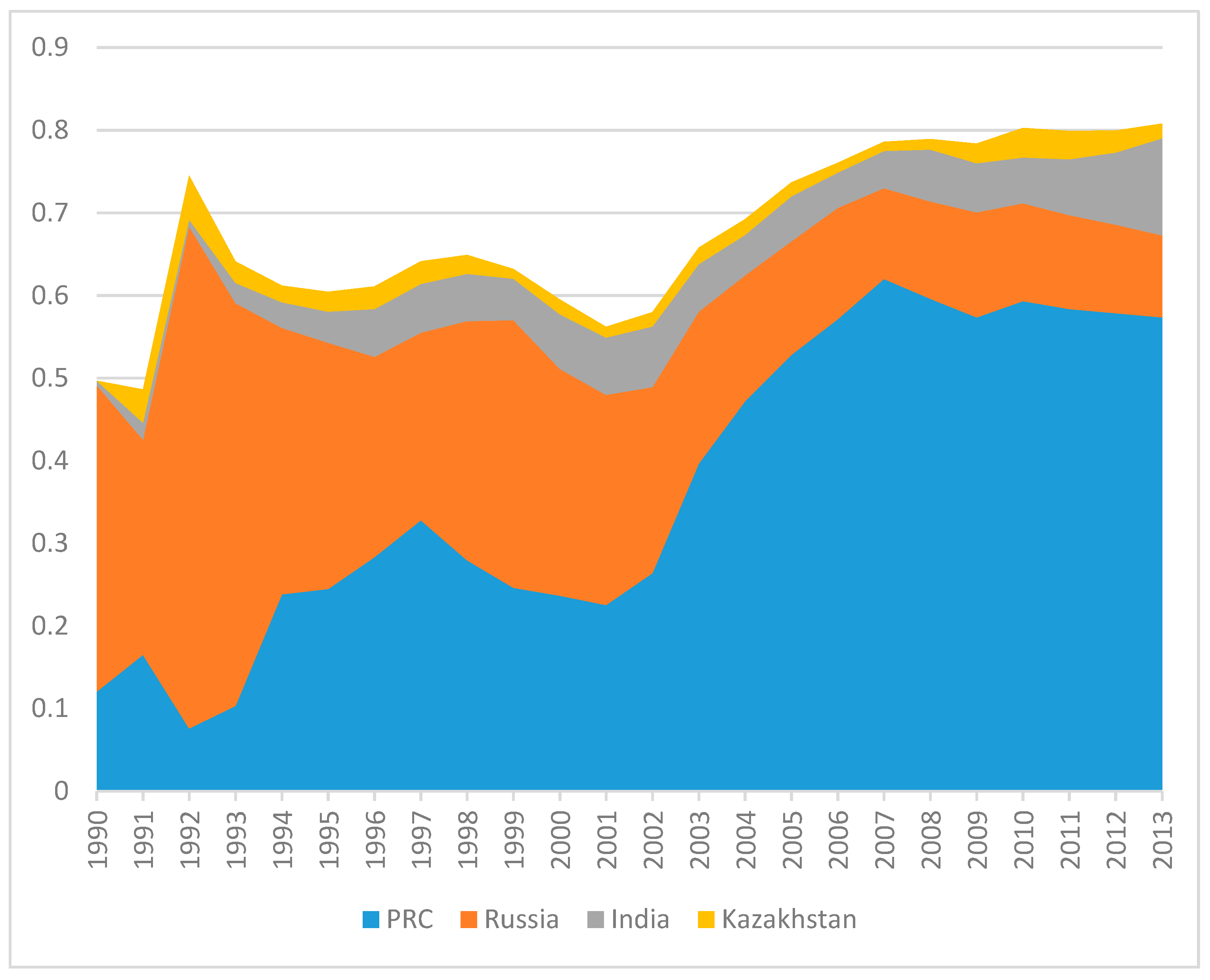
Figure 3.
Individual cross-section income elasticity estimates are plotted against the cross-sectional average GDP per capita (in natural logarithms) for the sample period. Territory-based carbon emissions is the dependent variable for (a) (top); consumption-based carbon emissions is the dependent variable for (b) (bottom). Second-order polynomial trend line, equation, and R-squared also shown.

Table 1.
Summary statistics. 20 countries, 1990–2013.
| Variables | Observations | Mean | Std. Dev. | Min | Max |
|---|---|---|---|---|---|
| GDP pc | 477 | $13,001 | 14,869 | $1011 | $77,721 |
| Log territory-based CO2 pc | 480 | 0.63 | 1.46 | −3.39 | 2.95 |
| Log consumption-based CO2 pc | 480 | 0.85 | 1.43 | −2.81 | 3.61 |
| Exports share | 472 | 52.1% | 49.0 | 5.9% | 230% |
| Imports share | 472 | 54.3% | 44.2 | 6.9% | 227% |
| Total fossil fuel share | 471 | 69.0% | 24.2 | 5.1% | 99.4% |
| Industry energy intensity | 465 | 889.5 | 2837.3 | 2.0 | 24,708.1 |
Table 2.
Cross-sectional dependence: Averaged absolute value correlation coefficients and Pesaran [28] CD test. 20 countries, 1990–2013, mostly balanced.
Table 2.
Cross-sectional dependence: Averaged absolute value correlation coefficients and Pesaran [28] CD test. 20 countries, 1990–2013, mostly balanced.
| Variables | CD-Test | Abs Corr. Coeff. |
|---|---|---|
| GDP pc | 60.9 * | 0.91 |
| Log territory-based CO2 pc | 23.7 * | 0.62 |
| Log consumption-based CO2 pc | 24.4 * | 0.57 |
| Exports share | 16.4 * | 0.52 |
| Imports share | 12.3 * | 0.44 |
| Total fossil fuel share | 10.8 * | 0.65 |
| Industry energy intensity | 5.1 * | 0.53 |
* p-value < 0.001. Null hypothesis is cross-sectional independence.
Table 3.
Pesaran [29] CIPS panel unit root test results. 20 countries, 1990–2013, mostly balanced.
Table 3.
Pesaran [29] CIPS panel unit root test results. 20 countries, 1990–2013, mostly balanced.
| Constant w/o Trend | Constant w/Trend | |||||||
|---|---|---|---|---|---|---|---|---|
| Number of Lags | ||||||||
| 0 | 1 | 2 | 3 | 0 | 1 | 2 | 3 | |
| Log GDP pc | 0.004 | 0.000 | 0.000 | 0.312 | 0. 924 | 0.129 | 0.006 | 0.998 |
| Log territory-based CO2 pc | 0.178 | 0.209 | 0.169 | 0.340 | 0.888 | 0.830 | 0.920 | 0.661 |
| Log consumption-based CO2 pc | 0.004 | 0.130 | 0.557 | 0.536 | 0.011 | 0.393 | 0.883 | 0.970 |
| Log Exports share | 0.241 | 0.949 | 0.982 | 0.999 | 0.010 | 0.946 | 0.798 | 0.998 |
| Log Imports share | 0.090 | 0.741 | 0.887 | 0.877 | 0.658 | 0.996 | 1.000 | 0.999 |
| Log Total fossil fuel share | 0.291 | 0.328 | 0.298 | 0.778 | 0.927 | 0.591 | 0.453 | 0.852 |
| Log Industry energy intensity | 0.336 | 0.695 | 0.802 | 0.995 | 0.370 | 0.811 | 0.593 | 0.888 |
Notes: p-values shown. Null hypothesis is the series is I(1).
Table 4.
Trade and carbon emissions. Pesaran [33] CCE-MG estimator.
Table 4.
Trade and carbon emissions. Pesaran [33] CCE-MG estimator.
| Dependent Variables | ||
|---|---|---|
| Independent Variables | Territory-Based CO2 pc | Consumption-Based CO2 pc |
| GDP pc | 0.64 *** [0.35 0.93] | 0.67 *** [0.34 0.99] |
| Fossil fuels share | 1.41 *** [0.62 2.21] | 1.04 *** [0.27 1.81] |
| Industry energy intensity | 0.13 * [0.02 0.25] | −0.004 [−0.13 0.13] |
| Exports share | 0.02 [−0.11 0.14] | −0.37 *** [−0.54 −0.21] |
| Imports share | 0.02 [−0.05 0.09] | 0.28 ** [0.08 0.48] |
| CD (p) | −1.0 (0.31) | −0.6 (0.52) |
| Order of integration | I(0) | I(0) |
Notes: Statistical significance level of 5%, 1% and 0.1% denoted by *, **, and ***, respectively. 95% confidence intervals in brackets. CD is the test statistic from the Pesaran [28] CD test; the corresponding p-value is in parentheses. The null hypothesis of the test is cross-sectional independence. Order of integration of the residuals is determined from the Pesaran [29] CIPS test: I(0) = stationary. Null hypothesis is I(1). Both regressions have 460 observations.
© 2018 by the author. Licensee MDPI, Basel, Switzerland. This article is an open access article distributed under the terms and conditions of the Creative Commons Attribution (CC BY) license (http://creativecommons.org/licenses/by/4.0/).
Share and Cite
MDPI and ACS Style
Liddle, B. Consumption-Based Accounting and the Trade-Carbon Emissions Nexus in Asia: A Heterogeneous, Common Factor Panel Analysis. Sustainability 2018, 10, 3627. https://doi.org/10.3390/su10103627
AMA Style
Liddle B. Consumption-Based Accounting and the Trade-Carbon Emissions Nexus in Asia: A Heterogeneous, Common Factor Panel Analysis. Sustainability. 2018; 10(10):3627. https://doi.org/10.3390/su10103627
Chicago/Turabian StyleLiddle, Brantley. 2018. "Consumption-Based Accounting and the Trade-Carbon Emissions Nexus in Asia: A Heterogeneous, Common Factor Panel Analysis" Sustainability 10, no. 10: 3627. https://doi.org/10.3390/su10103627
Note that from the first issue of 2016, this journal uses article numbers instead of page numbers. See further details here.