Influence of Natural and Anthropogenic Linear Canopy Openings on Forest Structural Patterns Investigated Using LiDAR

1
FPInnovations, 570 Boulevard Saint-Jean, Pointe-Claire, QC H9R 3J9, Canada
2
Centre for Forest Research, Department of Biological Sciences, University of Quebec in Montreal, P.O. Box 8888, Succ. Centre-Ville, Montreal, QC H3C 3P8, Canada
3
Natural Resources Canada, Canadian Forest Service, Laurentian Forestry Centre, 1055 rue du PEPS, P.O. Box 10380, Quebec City, QC G1V 4C7, Canada
*
Author to whom correspondence should be addressed.
Forests 2018, 9(9), 540; https://doi.org/10.3390/f9090540
Submission received: 20 July 2018
/
Revised: 27 August 2018
/
Accepted: 30 August 2018
/
Published: 2 September 2018
(This article belongs to the Special Issue Characterization and Regionalization of Disturbance Regimes Affecting Forests)
Abstract
:In much of the commercial boreal forest, dense road networks and energy corridors have been developed to access natural resources with unintended and poorly understood effects on surrounding forest structure. In this study, we compare the effects of anthropogenic and natural linear openings on surrounding forest conditions in black spruce stands (gap fraction, tree and sapling height, and density). Forest structure within a 100 m band around the edges of anthropogenic (roads and power lines), natural linear openings (streams), and a reference black spruce forest was measured by identifying individual stems and canopy gaps on recent high density airborne LiDAR canopy height models. CUSUM curves were used to assess the distance of edge influence. Forests surrounding anthropogenic openings were found to be gappier, less dense, and have smaller trees than those around natural openings. Forests were denser around natural and anthropogenic linear openings than in the reference forest with edge effects observed up to 24–75 m and 18–54 m, respectively, into the forest. A high density of saplings in the gappier forests surrounding anthropogenic openings may eventually lead to a higher forest biomass in the zone area surrounding roads as is currently observed around natural openings.
1. Introduction
As a consequence of the rapid increase in forest management and resource extraction, an increase in the abundance of narrow-linear canopy openings such as roads, powerlines, oil and gas pipelines, etc. can be observed over the past century in forested areas throughout the world [1]. Road networks now criss-cross much of the temperate and boreal forest regions. For example, in the United States there are more than 6.3 million km of roads in forests [2], British Columbia (Canada) has an estimated total of 400,000–550,000 km of unpaved forest roads [3], and Quebec annually builds an estimated 4000–5000 km of forest roads [4]. In order to understand their overall impact on the forest, it is necessary to evaluate the distance of influence of edge effects from these openings. Earlier studies have reported a large array of distance effects from edges ranging from tens to thousands of meters depending on the metric evaluated and the study region [5,6,7]. Linear openings have a high edge to area ratio which given their omnipresence should lead to large effects across vast managed forest regions.
As with other openings, linear corridors cause breaks in otherwise continuous interior forest habitat thereby creating an abrupt forest edge where ecological changes in energy flow, wildlife movement, seed dispersal, and abiotic conditions occur [6,7,8]. Changes in abiotic conditions affect forest structure and composition through increased edge-tree mortality and/or seedling recruitment that can further influence the original abiotic edge effect [6,9,10]. Increases in resources such as light could also lead to greater tree growth and thus higher forest productivity [11,12] or greater structural diversity [13] adjacent to edges. These effects on adjacent vegetation, depending on the distance of the effects, have influences on both wildlife habitat and forestry (i.e., increased mortality vs. increased growth) [14,15]. The intensity and distance of edge effects is influenced by attributes such as age, history, type, and orientation of the linear openings. Burton [16] has also shown that the geographic position or orientation, especially North vs. South sides of an opening, affects forest stem density.
In recent years there has also been an emphasis on minimizing the difference between the effects of natural and anthropogenic disturbances on forests in order to maintain ecological processes and biodiversity [17]. This is based on the precept that organisms are adapted to conditions that have occurred naturally for thousands of years [18]. In the case of comparing forest harvesting to natural disturbances, recent years have seen a wealth of information developed. However, as important as roads and other anthropogenic linear openings are in dissecting forests, little understanding has been developed as to their similarities and differences with natural linear opening such as streams. In many forested regions, natural linear openings, such as streams, are abundant. Forest surrounding these openings established in their presence whereas anthropogenic openings were cut into pre-existing forest. The initial forested condition, i.e., natural forest dissected by anthropogenic openings or forest that developed around liner features such as streams, may influence tree response. With this in mind, we thus ask whether anthropogenic linear openings (roads and power lines) are analogues to streams in terms of their effects on surrounding forest conditions. Further, we assess how far effects on forest structure (density, height, gap fraction, and regeneration) extend into the surrounding forests and if they vary according to opening type (natural or anthropogenic).
Edge effects are usually measured on-site, using transects and sampling plots as a basis for determining changes in vegetation composition or function [10,13,19]. As linear openings cover long distances across a landscape, it can be difficult to acquire comprehensive tree and canopy level information for a wide band of adjacent forests, using on-site measurements. This may limit our ability to confidently estimate the full extent of edge affected area, as well as characterizing their cumulative impact, with researchers forced to study a small number of plots instead of large continuous areas. To understand change from the edge-to-interior gradient, it is important to capture the variability along a continuous and sufficiently long distance parallel to the edge in question instead of making discrete measurements along a transect. Remote sensing may contribute to resolve these limitations, as it covers contiguous forested area. In recent years, Light Detection and Ranging (LiDAR) have offered promising ways to obtain detailed information on vegetation structure at several vertical and horizontal scales [20,21,22]. To replace discontinuous ground observations, we thus use canopy height models (CHM, a surface describing the distribution of canopy height across space) generated from high density discrete LiDAR to extract individual stem measurements and canopy gaps.
2. Methods
2.1. Study Area
The study area is located in the Quebec North Shore region (49°30′–50°00′ N; 67°30′–69°00′ W), (Figure 1a). The closest meteorological station is at Baie-Comeau, 50 km south of the study area. The climate is considered cold and maritime with a mean annual temperature of 1.4 °C and a mean annual precipitation of 1018 mm where 70% of this total occurs as rainfall [23]. Topography is characterized as hilly with moderate slopes (<30%). Summits are rounded or mostly flat, with elevation varying between 500–700 m. Rocky outcrops occupy close to 40% of the area and are present on summits, close to water bodies, and on steep slopes. Undifferentiated glacial tills constitute the majority of the remaining surficial deposits and are found on gentle slopes and in depressions. Glacial fluvial sand deposits occupy the bottom of large valleys along rivers [23].
The study area overlaps the Abies balsamea-Betula papyrifera and Picea mariana-moss bioclimatic domains [24] and is within the Chibougamau-Natashquan boreal region [25]. Picea mariana and Abies balsamea are the dominant species in this area. A. balsamea is dominant on mesic sites in the southern part of the range along with B. papyrifera and Populus tremuloides. P. mariana becomes more frequent as latitude increases. Pinus banksiana is a minor species found primarily on sandy soils [23]. The fire cycle is close to 300 years [26] and spruce budworm outbreaks were historically not severe in the region [27,28]. Thus, a large proportion of the area is dominated by old-growth forests, where gap dynamics are driving changes in structure and composition [29]. Gaps generally result from the mortality of a small number of trees and most are smaller than 100 m2 [29]. Although logging dates to the early 1930’s throughout the study area (including the LiDAR flown study sites) large patches of untouched forests (>150 km2) dominate.
2.2. LiDAR Data
LiDAR data were acquired on 19 June 2010 using an Optec-ALTM 3100 flown at 700 m with a pulse frequency of 100 kHz, a maximum scan angle of 15°, a footprint size of 21 cm, and an average overall return density of 7 hits/m2 were used. This multireturn dataset was calibrated and then classified following the American Society for Photogrammetry and Remote Sensing guidelines using the TerraScan algorithm by the data provider. The canopy height models (CHM) and LiDAR-derived three-dimensional surfaces that are the vegetation height above the ground surface (Figure 1b–e) of the study forest were generated by calculating the difference between the elevations of the respective canopy surface (digital surface model, DSM) and the underlying terrain (digital terrain model, DTM). DSM and DTM of 0.25 m resolution were created following the method explained in Vepakomma et al. [21].
2.3. Site Selection
We identified anthropogenic and natural linear openings within a LiDAR sample area flown in 2010. The anthropogenic openings were composed of roads and powerline corridors and the natural ones were streams. Powerlines were established in the early 1960s and are wider (90–150 m) than roads (approximately 20 m width). We considered old roads that were established in the late 1950’s to connect Baie-Comeau to the Ste-Anne Reservoir. In this study we sampled 10 ha of contiguous forest bands per linear opening (5 ha on each side of the opening for a minimum length of 500 m parallel to it and running 100 m from the edge of the opening into the forest) (Figure 1e). In the LIDAR data set, two sites for streams and powerlines and three sites for roads, covering a minimum of 16 ha of contiguous forests in each, were available for the analyses. An area of 16 ha of contiguous old-growth forest was considered sufficiently large to encompass the variability generated by gap dynamics, since more than 80% of gaps are smaller than 100 m2 [29]. Thus, such an area would be representative of most of the regional variability observed in old-growth forest, while giving the advantage of analyzing contiguous forest area to detect finer scale transitions in forest structural characteristics.
Sites were carefully selected (i) within old growth forests, (ii) on relatively level terrain, (iii) fairly linear with consistent width, (iv) openings that are at least 50 years old, and (v) at least a 300 m distance from large water bodies and any major disturbances (Table 1, Figure 1a). We used all areas falling within the LiDAR acquired region matching the set of criteria presented above. A total of 106 ha of forested area adjoining the linear openings were sampled. In addition to the linear openings, a separate window of size 400 m × 400 m (16 ha) within old-growth forests was selected as a reference forest to describe interior forest conditions in the absence of linear openings (Figure 1a).
Since edge effects are expected to be directionally asymmetrical at high latitudes, and wherever winds have a predominant direction [30,31], we also analyzed forest conditions on both sides of each linear opening. Orientation of the linear opening was measured by its inclination from the north (Table 1). “North” refers to the northern fragment of the forest adjoining the opening and hence south-facing to the linear opening.
2.4. Data Analysis
2.4.1. Response Variables and Buffer Segments
The influence of linear openings on the adjoining forest was assessed for the following structural variables: overstory structure (average tree height, tree density per ha) and regeneration (average sapling height, sapling density per ha) gap fraction. The effect of the edge-to interior gradient on the adjoining forest was assessed using 50 multi-ring buffers of 2 m width each, parallel to the linear openings. This was done on each side of the linear opening with the use of ArcGIS. The most frequent crown width of the trees sampled was chosen as the buffer segment width (2 m), and over six times the average stem height as the maximum distance to be sampled from a linear opening into the interior forest i.e., 100 m.
A stem was considered as a tree if it reached a minimum height of 4 m; otherwise it was a sapling. Average tree and sapling height, tree and sapling density (standardized per ha), and gap fraction, were calculated for each buffer segment. The buffer polygon segments were used to estimate the structural (response) variables along the distance gradient as described below:
Average stem height:
Stem density/ha:
Gap fraction:
where tij, i = 1 to nj, ith tree height in the jth segment which has nj identified canopy trees; Aj: area (in m2) within the jth segment; Gij is the area under the ith gap in the jth segment.
2.4.2. Individual Tree Identification and Validation
Individual trees were located by first identifying tree tops using local maxima filtered on a Gaussian smoothed CHM and then by delineating the crowns by adopting a marker controlled watershed segmentation on the complement of the CHM [32,33,34]. Local maxima filtering of 0.5 m radius (based on smallest tree size) moving window was used on a Gaussian smoothed CHM to identify markers for segmentation. After segmentation was performed, the position and height of the highest LiDAR return within each tree segment were used as the location of single tree tops and their maximum tree height. A sample of automatically segmented tree stems is shown in Figure 2b.
Independent validation of stem identification and tree height using this algorithm for stands in a mixedwood boreal forest [32]. A similar validation was carried out in this study area showed 87.8% identification accuracy and a strong acceptance with an R2 = 0.95, r2 = 0.97, and RMSE = 0.94 m of tree height (see Supplementary Materials for more details).
2.4.3. Gap Definition and Delineation
A gap was defined as an area within the forest where crown heights of the tallest stems were noticeably lower than the height of the adjacent canopy [35]. This is assumed to be due to the death of a single or group of trees. Other types of openings such as water bodies, roads, and rock outcrops were not treated as gaps. They were eliminated by applying a minimum canopy height of 0.5 m (a threshold verified independently against high resolution images). Gaps were identified by the absence of trees in the canopy such that the height of any remaining stems was lower than a given absolute height (gh). The gh threshold was fixed based on the canopy height where the relative increase in proportional closed canopy area reaches a maximum and then tends to stabilize. From available ground tree measurements, and LiDAR surfaces of two forested test sites of size 25 ha each within the region, gh was estimated to be 4 m. Individual canopy gaps were then delineated by adopting the automated algorithm described in Vepakomma et al. [21]. Figure 2c presents an example of the automatically delineated gaps in the adjoining remnant forests along the linear openings.
2.4.4. Comparison of Forests around Linear Openings and Reference Forest
Differences in forest structure were tested using Kolmogorov–Smirnov and Mann–Whitney U nonparametric two-sample tests. To assess whether the response variable along the edge-to-interior gradient is significantly different from that of the reference forest, we estimated 95 percent confidence intervals (2.5th and 97.5th percentiles) for each of the variables based on their response in the reference forest. The 16 ha reference forest was divided into 1600 sub-plots of size 100 m2. To remove any sampling bias, we then extracted three sets of 5000 bootstrapped samples of size 1600 (using simple random sampling with replacement) independently for (1) the total number of saplings and total sapling height, (2) the total number of trees and total tree height, and the (3) total gap area. The 2.5th and the 97.5th percentiles of the response variables and 95% confidence intervals were then estimated using their respective 5000 bootstrapped values. Mean values of the response variable along the edge-to-interior gradient of linear opening were considered significant if they were outside the confidence interval of the reference forest.
2.4.5. Depth of Influence—Average CUSUM
To determine the extent of a linear opening’s influence (Depth of influence, DEI) and to find thresholds of changes, we plotted the average cumulative sums (CUSUMs) of the response variable against the distance from the edge of a linear opening. CUSUM methods are process control statistical techniques used to determine changes or shifts over time in a process [36]. More recently to create zones of influence of canopy gap opening on the structure of the surrounding boreal forest matrix [33]. Control charts usually do not detect small shifts in a process, observed say by measuring a change in statistic Q from a desired value k, instead these small shifts appear more like noise around the mean. On the other hand, the slope of the curve from the cumulative sum of such small shifts (as defined below), may be more indicative of how average Q differs from k.
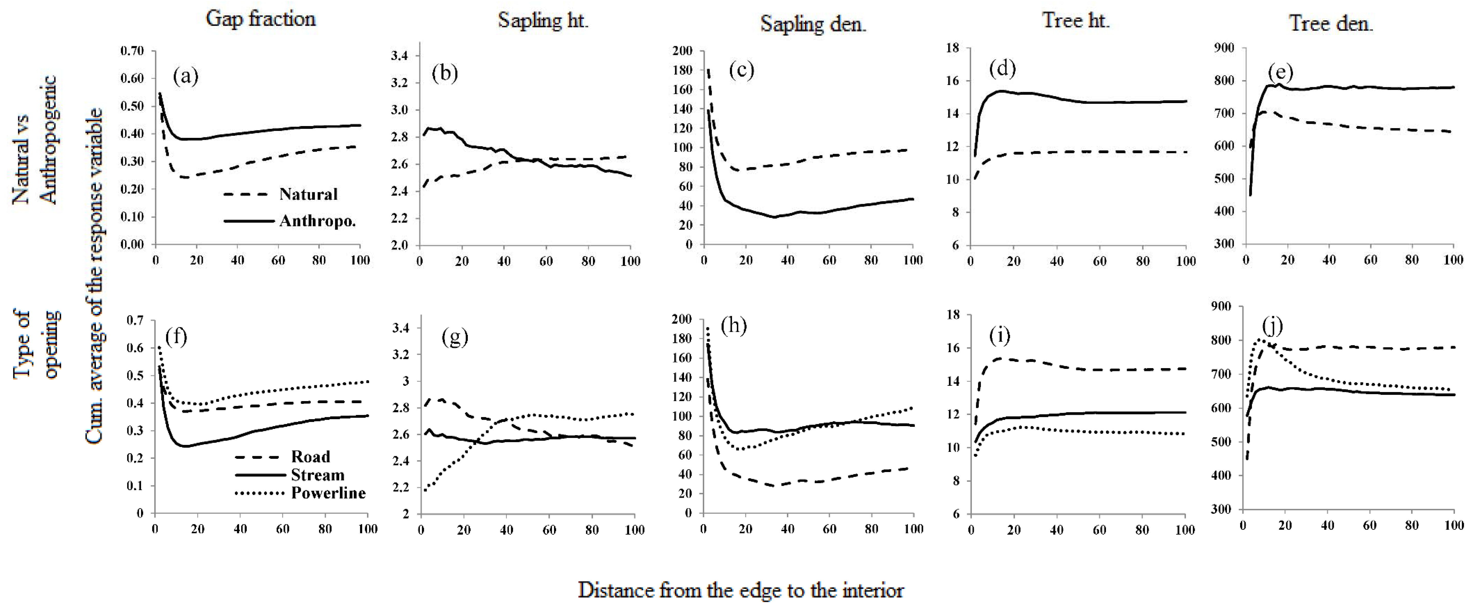
By estimating the cumulative average of a response variable along the distance from the edge (CUAVG) the depth of influence of the linear opening on the adjacent forest is established. The point where the rate of change of CUAVG of the response variable converges to zero is considered to be the distance at which the explanatory variable, and hence the linear opening edge, ceases to have an influence on changes in the response variable.
CUAVGj,i, the average of the cumulated value of the jth response variable up to the ith distance from the edge is computed as given below.
CUAVG of average stem height:
where Nk is total number of stems up to the kth segment, yi, is the total tree height of all the stems in the ith segment, and Ti−1 is the total tree height of Nk−1 stems up to the (i − 1)th distance from the edge.
CUAVG of stem density:
where Ak is total area (in m2) up to the kth segment, ni is the total number of stems in the ith segment, and Ni − 1 is the total number of stems up to the (i − 1)th distance from the edge.
CUAVG of gap fraction:
where Ak is total area (in m2) up to the kth segment, yi is the total area in gaps in the ith segment, and Ti−1 is the total area in gaps up to the (i − 1)th distance from the edge.
2.4.6. Magnitude of Edge Influence MEI
Independently, for each of the response variables we also calculated the magnitude of edge influence (MEI). MEI is a measure of the extent to which a given parameter differs at the edge as compared to the forest interior (Harper et al. 2005). MEI of the jth response variable is computed as:
where e is the value of the parameter at the edge of the linear opening, i is the value of the parameter of the jth response variable in the interior forest, and −1 < MEI < 1, with positive values indicating a positive response to the linear opening, negative values a negative response and zero indicating no response.
3. Results
3.1. Reference Forest vs. Forests around Linear Openings
We evaluated the influence of linear openings on forest structure as measured by canopy gaps, sapling height and density, and tree height and density along a 100 m wide forest band. These were compared to a reference forest. Forest structure significantly differed in the neighborhood of linear openings compared to the reference forest (pairwise Kruskal–Wallis ANOVA by ranks, p < 0.001, Table 2).
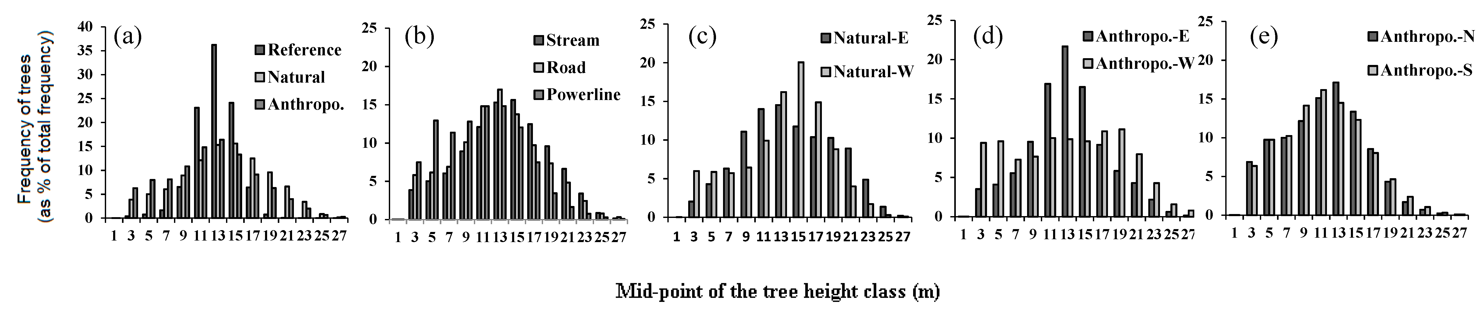
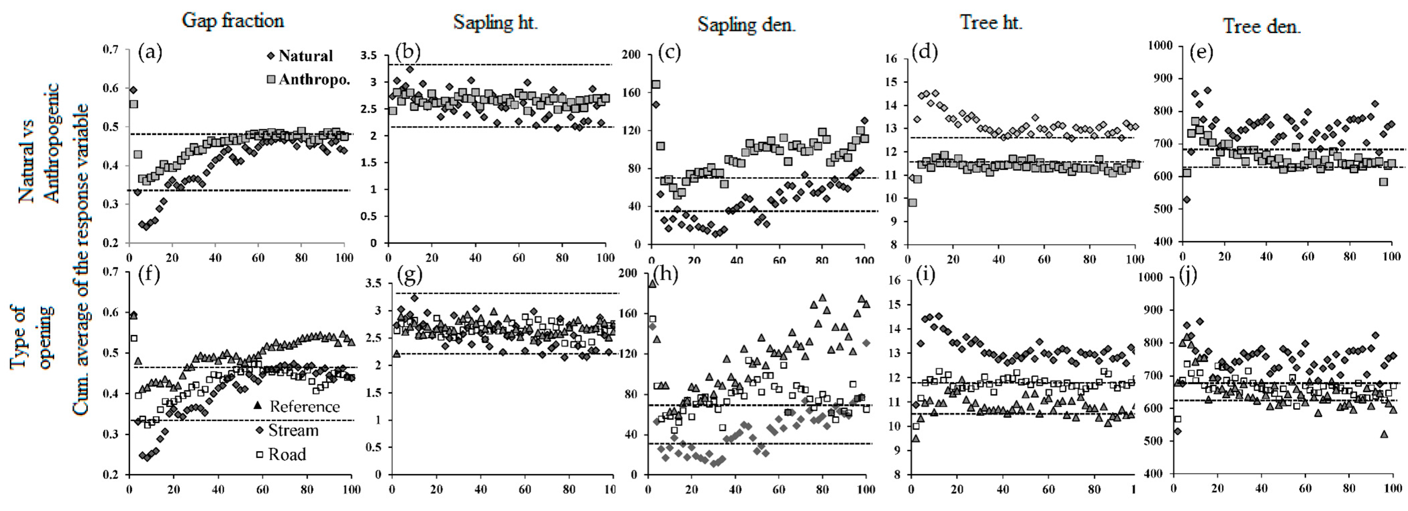
Reference forests have an average height of 11.93 m, a density of 520 trees/ha and 36 saplings/ha, and a gap fraction of 36%. As compared to reference forests, forests around natural linear openings were taller while around anthropogenic ones they were shorter. Both natural and anthropogenic openings had denser and more disturbed surrounding forests, as compared to reference forests (Table 2). Tree height in the reference forest is normally distributed with a peak around 12–14 m. In these forests, 98% of the trees are higher than 10 m, of which 90% are between 10–16 m (Figure 3). Tree height distribution in the vicinity of linear openings was significantly different from the reference forest (Table 2). In the reference forest tree height distribution tended to be unimodal, narrower, and peaked, whereas for all types and aspects of linear openings tree heights occurred across a wider range (p < 0.001, Figure 3a,b). Tree height distribution on either side of natural openings is skewed more to the left compared to the reference forest, with over 50% of the trees more than 16 m in height (Figure 3c). In comparison, for anthropogenic openings, with the exception of western orientations, distributions appear mostly uniform (Figure 3d,e). In these forests, over 40% (but about 20% in the western aspect) of the trees were below 10 m in height. Furthermore, with the exception of sapling height, all response variables in all linear opening types were significantly beyond the range of variability of the reference forests generated from the bootstrap analysis (Figure 4). Compared to reference forests and irrespective of the type of opening, gap fraction, sapling, and tree density were positive and increased in magnitude with opening width whereas, sapling height, and to a lesser extent tree height, responded negatively (Figure 4a).
Canopy gaps are more frequent in forests along the edge-to-interior gradient for all linear opening types (stream, road, and powerline) compared to the reference forest (Table 2, Figure 4). There are fewer saplings close to any type of linear opening but the number of saplings is heterogeneous and consistently increases with distance from the edge (Table 2, Figure 4). Comparing the distribution of each response variable with respect to the critical intervals, only sapling density and gap fraction up to 40 m in all linear opening types significantly matched the reference forest. On the other hand, average sapling height in the reference forest is slightly higher than what is observed in the forests around linear openings and hence has a negative MEI (Figure 5).
3.2. Natural vs. Anthropogenic Openings
Forest structure significantly varied around natural and anthropogenic linear openings. Gap fraction, sapling height, and sapling density were significantly greater near anthropogenic openings whereas, tree height and tree density were significantly greater in forests adjacent to natural openings (Table 2). Although, there was no consistent difference of one orientation affecting structural characteristics more than the other, the western side not only had greater gap fraction and sapling density for both anthropogenic and natural openings, but also greater tree density and tree height around anthropogenic openings (Table 2 and Table S1 and Figure 4). Sapling height for both anthropogenic and natural and tree height for natural openings was, in contrast, greater on the eastern side of the openings. Differences between northern and southern aspects around anthropogenic linear openings were not pronounced for any of the structural variables measured (Table 2).
The variation in the structural indices evaluated is especially large in the first 20–30 m from the edge of the opening. Although forests around roads have similar average structural characteristics to forests around natural openings, distributions along distance from the edge are significantly different (KW test, p < 0.01, Table 2 and Figure 4). Forests around power line corridors are shorter in height, more disturbed with a gap fraction of almost 50% and an average tree height below 11 m (Table 2). The MEI of tree height and density around anthropogenic openings was negative with respect to natural ones (Figure 5b). Sapling height was not affected by the type of opening or the orientation.
The depth-of-edge influence (DEI) varied considerably among the response variables, from as close as 15 m to almost 80 m deep into the forest (Table S1, Figure 6). Although effects can extend a long distance, changes in most structural indices are greatest in the first ten to fifteen meters from all types of linear openings (Figure 6). The exception to this observation is for sapling height which continues to change rapidly out to or past 40 m for different opening types. However, the rate of change of DEI between 10 and 20 m differed between natural and anthropogenic openings for all the response variables. A high tree density in proximity to the edges (within 10–15 m) resulted in a negative change in the slope of the CUAVG curve in tree height and density. Similarly, increased occurrence of gaps 10 m from the edges resulted in high positive change in the slope of CUAVG curves of gap fraction and sapling density. In general, the impact of natural openings penetrates deeper into the forest than that of anthropogenic openings. Irrespective of the type of the opening, DEI is generally further for gap fraction and sapling density in the western aspect (Figure 6, Table S1 and Figure S1).
4. Discussion
Disturbance is considered an integral factor shaping the structural characteristics of boreal forests [17,30]. In the case of natural disturbances, the impact of small scale disturbances may vary over short temporal and spatial scales [30,33]. Human-caused disturbances, on the other hand, may induce more severe and sometimes longer-lasting effects on the forest [6,37,38]. As anthropogenic linear openings such as roads and powerlines are becoming dominant features in forested landscapes in many parts of the boreal forest it is critical that we evaluate their potential effects on forest structure.
A limitation of this study, as with all studies, is that specific measurements may be particular to the study region. Absolute values, in this study as in others, reflect the productivity of soils, climatic conditions, forest composition, etc. However, in contrast with field studies which are based on a number of small plots or transects located in a region, we analyze all data from all contiguous forest areas around the linear openings available in the LIDAR data set for our study and use bootstrapping in the statistical analyses. Nonetheless, we acknowledge that this work should be repeated in other forested landscapes to evaluate its generalizability. Despite these limitations, our results demonstrate marked changes in forest structure in the proximity of linear openings when compared to the reference forest, and also differences in structure surrounding natural and anthropogenic linear openings. Furthermore, many of the results, although not always intuitive, are consistent with ecological processes. Forests were taller around older natural linear openings but shorter around younger anthropogenic ones, while forests around both were denser, probably due to greater light, than in reference forests.
Since anthropogenic linear openings were created 50 to 60 years ago, we could interpret differences with natural forests as meaning that forests in the vicinity of anthropogenically created openings are still responding to the effects of the initial disturbance. Structural heterogeneity varied up to 18–54 m in the forests around linear anthropogenic openings in this study; which is similar to the distance impacts that have been reported on the vegetation around harvest blocks in boreal forests [16,39], but less than that reported for harvested tropical forests [40,41].
4.1. Do Natural and Anthropogenic Linear Openings Cause the Same Effects?
Amongst the structural differences that we noted; the forests surrounding anthropogenic openings have a higher gap fraction than around natural openings. Anthropogenic linear developments open otherwise continuous interior forest habitat creating an abrupt forest edge where wind and other stresses on trees increase [6,37]. Studies on windthrow following strip-cutting, of similar widths to the linear openings of this study, showed that tree mortality varied from 20 to 30% in the neighboring forests in the early years following disturbance [42,43]. The relatively permanent nature of natural stream openings may on the other hand reduce canopy disturbance as surrounding vegetation is adapted to the edge conditions [44,45,46]. Future studies should thus investigate the temporal dynamics of forest road establishment on surrounding forest structural characteristics. This would allow us to better understand how and if the effect stabilizes with time elapsed since road creation. Nonetheless, the greater abundance of openings (gap fraction) around anthropogenic openings led to an increase in sapling density. As these young stems grow in size they will reduce the openness of the surrounding forest.
4.2. The Influence of Orientation
Orientation of the edge determines the amount of exposure to solar radiation and impact of wind, and hence may considerably modulate the impact [16]. North facing edges in south-eastern Pennsylvania exhibited milder microclimate effects, elevated irradiance in the forest understory in south-facing edges to distances of approximately 65 to 70 m [47]. However, in our study we only found a consistent effect of orientation in proximity to the anthropogenically created linear openings where most structural factors studied increased on the western side. The greater gap fraction may have led to increases in tree growth, and tree and sapling density.
4.3. How Far Do Effects Extend?
In this study we identified effects of roads on forest structure to distances greater than reported in other boreal literature [46]. Given the positive influence of linear openings on tree height and density out to distances of 60 m on either side of the opening and given the vast network of forest roads, forest management is having an unintended influence on forest productivity. With edge effects of up to 120 m (60 m on both sides), more than 10 ha of forest are influenced per 1 km of road. With tens of thousands of kilometer’s of forest roads constructed annually [1] the changes in productivity of forest stands are easily on the order of hundreds of thousands of hectares per year. As well as increases in tree height and tree density there is also greater mortality as evidenced by the increase in gap fraction adjacent to roads. It will thus be critical in the future to fully evaluate the overall balance of the positive effects on growth and biomass with the increased mortality. However, our results on tree density show that there is a greater number of trees per unit area in the forests surrounding the linear openings than in the reference forests and these results include the presence of gap openings. The greater number of trees and their greater height thus imply that there should be a greater volume of wood in proximity to linear openings such as roads. This would be consistent with other findings that vegetation productivity increased up to 50 m into the forests adjacent to roads [11,12]. Thus despite their negative impacts on wildlife [37,48] and on indigenous culture [49] roads may have unintended positive effects on the growth and productivity of surrounding forests.
5. Conclusions
The vast linear network of openings created due to road building and energy transport is having unplanned influences on surrounding forests. This study demonstrates that forest structure around linear openings is different than in undisturbed forest and that there are differences between natural linear openings such as streams and anthropogenically created ones such as roads and powerlines. Previously identified negative effects of roads on wildlife may at least in part be balanced by increased productivity from sapling recruitment to the tree layer. However, this increase in productivity may not compensate the permanent loss in tree volume, associated with tree removal for road and powerline construction. The construction of nonpermanent roads could in the long term have positive effects both on forest productivity and wildlife.
This work adds to the existing evidence that LiDAR offers an effective and rapid means of capturing fine-scale heterogeneity as well as determining the cumulative impact of both anthropogenic and natural linear disturbances in the forests. This enlarges the scope for forest managers and conservation biologists by providing a deeper understanding of landscape fragmentation, spatial heterogeneity, and vegetation patterns across multiple-scales.
Supplementary Materials
The following are available online at https://www.mdpi.com/1999-4907/9/9/540/s1. Figure S1: Depth of influence (DEI) of selected types of linear openings on either sides of the adjoining forest shown by CUAVG curves of response variables against the distance from the edge of a linear opening. (a–e) DEI on either sides of natural linear openings; (f–j) DEI on either sides of anthropogenic linear openings, Table S1: Depth of edge influence (m) of the selected linear openings into the adjacent forest determined based on the slope of the CUSUM curve.
Author Contributions
U.V., D.K., and L.D. designed the study. U.V. did all the statistical analyses and wrote the methods and results sections. All authors contributed to the introduction and the discussion.
Funding
This research was funded by Le Fond de Recherche sur la nature et les technologies (FQRNT) and the National Scientific and Engineering Research Council of Canada (NSERC) for financial support to Vepakomma and Kneeshaw respectively.
Acknowledgments
The authors would like to thank Benoit St-Onge (UQAM), Robert Schneider (UQAR), and Dominique Boucher (NRCAN) for their help with the data acquisition for this research. We also thank the MRNF North-Shore region (SM3Fund) for their financial support in LiDAR data acquisition and processing. We acknowledge valuable discussions with Karen Harper. Finally we would like to thank two anonymous reviewers for their helpful comments on a prior version of this manuscript.
Conflicts of Interest
The authors declare no conflicts of interest.
References
- Bourgeois, L.; Kneeshaw, D.; Boisseau, G. Les routes forestières au québec: Les impacts environnementaux, sociaux et économiques. VertigO-La Rev. Électron. Sci. L’environ. 2005, 6, 2. [Google Scholar] [CrossRef]
- Riitters Kurt, H.; Wickham James, D. How far to the nearest road? Front. Ecol. Environ. 2003, 1, 125–129. [Google Scholar] [CrossRef]
- Daigle, P. A summary of the environmental impacts of roads, management responses, and research gaps: A literature review. J. Ecosyst. Manag. 2010, 10, 65–89. [Google Scholar]
- Coulombe, G.; Huot, J.; Arsenault, J.; Bauce, E.; Bernard, J.-T.; Bouchard, A.; Liboiron, M.A.; Szaraz, G. Commission D’étude sur la Gestion de la Forêt Publique Québécoise; Bibliothèque Nationale du Québec: Québec City, QC, Canada, 2004; p. 307. [Google Scholar]
- Alverson, W.S.; Waller, D.M.; Solheim, S.L. Forests too deer: Edge effects in northern Wisconsin. Conserv. Biol. 1988, 2, 348–358. [Google Scholar] [CrossRef]
- Gascon, C.; Williamson, G.B.; da Fonseca, G.A.B. Receding forest edges and vanishing reserves. Science 2000, 288, 1356–1358. [Google Scholar] [CrossRef] [PubMed]
- Laurance, W.F.; Goosem, M.; Laurance, S.G.W. Impacts of roads and linear clearings on tropical forests. Trends Ecol. Evol. 2009, 24, 659–669. [Google Scholar] [CrossRef] [PubMed] [Green Version]
- Forman, R.T.T.; Godron, M. Landscape Ecology; Jhon Wiley & Sons: New York, NY, USA, 1986; p. 619. [Google Scholar]
- Williams-Linera, G. Vegetation structure and environmental conditions of forest edges in Panama. J. Ecol. 1990, 78, 356–373. [Google Scholar] [CrossRef]
- Murcia, C. Edge effects in fragmented forests: Implications for conservation. Trends Ecol. Evol. 1995, 10, 58–62. [Google Scholar] [CrossRef]
- Johnson, H.B.; Vasek, F.C.; Yonkers, T. Productivity, diversity and stability relationships in mojave desert roadside vegetation. Bull. Torrey Bot. Club 1975, 102, 106–115. [Google Scholar] [CrossRef]
- Lamont, B.B.; Rees, R.G.; Witkowski, E.T.F.; Whitten, V.A. Comparative size, fecundity and ecophysiology of roadside plants of banksia hookeriana. J. Appl. Ecol. 1994, 31, 137–144. [Google Scholar] [CrossRef]
- Harper, K.A.; Macdonald, S.E. Structure and composition of riparian boreal forest: New methods for analyzing edge influence. Ecology 2001, 82, 649–659. [Google Scholar] [CrossRef]
- Kardynal, K.J.; Morissette, J.L.; Van Wilgenburg, S.L.; Bayne, E.M.; Hobson, K.A. Avian responses to experimental harvest in southern boreal mixedwood shoreline forests: Implications for riparian buffer management. Can. J. For. Res. 2011, 41, 2375–2388. [Google Scholar] [CrossRef]
- Arienti, M.C.; Cumming, S.G.; Krawchuk, M.A.; Boutin, S. Road network density correlated with increased lightning fire incidence in the Canadian western boreal forest. Int. J. Wildland Fire 2009, 18, 970–982. [Google Scholar] [CrossRef]
- Burton, P.J. Effects of clearcut edges on trees in the sub-boreal spruce zone of northwest-central British Columbia. Silva Fenn. 2002, 36, 329–352. [Google Scholar] [CrossRef]
- Gauthier, S.; Vaillancourt, M.-A.; Leduc, A.; De Grandpré, L.; Kneeshaw, D.; Morin, H.; Drapeau, P.; Bergeron, Y. Ecosystem Management in the Boreal Forest; Presses de l’Université du Québec: Québec, QC, Canada, 2009; p. 539. [Google Scholar]
- Angelstam, P.K. Maintaining and restoring biodiversity in european boreal forests by developing natural disturbance regimes. J. Veg. Sci. 1998, 9, 593–602. [Google Scholar] [CrossRef]
- Didham, R.K.; Lawton, J.H. Edge structure determines the magnitude of changes in microclimate and vegetation structure in tropical forest fragments. Biotropica 1999, 31, 17–30. [Google Scholar] [CrossRef]
- Kane, V.R.; Gersonde, R.F.; Lutz, J.A.; McGaughey, R.J.; Bakker, J.D.; Franklin, J.F. Patch dynamics and the development of structural and spatial heterogeneity in pacific northwest forests. Can. J. For. Res. 2011, 41, 2276–2291. [Google Scholar] [CrossRef]
- Vepakomma, U.; St-Onge, B.; Kneeshaw, D. Spatially explicit characterization of boreal forest gap dynamics using multi-temporal lidar data. Remote Sens. Environ. 2008, 112, 2326–2340. [Google Scholar] [CrossRef]
- Vierling, K.T.; Vierling, L.A.; Gould, W.A.; Martinuzzi, S.; Clawges, R.M. Lidar: Shedding new light on habitat characterization and modeling. Front. Ecol. Environ. 2008, 6, 90–98. [Google Scholar] [CrossRef]
- Robitaille, A.; Saucier, J.P. Paysages Régionaux du Québec Méridional. Direction de la Gestion des Stocks Forestiers et Direction des Relations Publiques, Ministère des Ressources Naturelles du Québec; Les Publications du Québec: Québec, QC, Canada, 1998. [Google Scholar]
- Thibault, M.; Hotte, D. Les Régions Écologiques du Québec Méridional: Deuxième Approximation; Ministère de L’énergie et des Ressources, Service de la Cartographie: Québec, QC, Canada, 1985. [Google Scholar]
- Rowe, J.S. Forest Regions of Canada; Service, C.F., Ed.; Fisheries and Environment Canada: Ottawa, ON, Canada, 1972; p. 172. [Google Scholar]
- Bouchard, M.; Pothier, D.; Gauthier, S. Fire return intervals and tree species succession in the north shore region of Eastern Quebec. Can. J. For. Res. 2008, 38, 1621–1633. [Google Scholar] [CrossRef]
- Blais, J.R. Les forêts de la côte nord au québec sont-elles sujettes aux déprédations par la tordeuse? For. Chron. 1983, 59, 17–20. [Google Scholar] [CrossRef]
- Bouchard, M.; Pothier, D. Spatiotemporal variability in tree and stand mortality caused by spruce budworm outbreaks in eastern Quebec. Can. J. For. Res. 2010, 40, 86–94. [Google Scholar] [CrossRef]
- Pham, A.T.; Grandpré, L.D.; Gauthier, S.; Bergeron, Y. Gap dynamics and replacement patterns in gaps of the northeastern boreal forest of Quebec. Can. J. For. Res. 2004, 34, 353–364. [Google Scholar] [CrossRef]
- Kneeshaw, D.D.; Bergeron, Y. Spatial and temporal patterns of seedling and sapling recruitment within canopy gaps caused by spruce budworm. Ecoscience 1999, 6, 214–222. [Google Scholar] [CrossRef]
- Canham, C.D.; Denslow, J.S.; Platt, W.J.; Runkle, J.R.; Spies, T.A.; White, P.S. Light regimes beneath closed canopies and tree-fall gaps in temperate and tropical forests. Can. J. For. Res. 1990, 20, 620–631. [Google Scholar] [CrossRef]
- Vepakomma, U.; Schneider, R.; Berninger, F.; Mailly, D.; St-Onge, B.; Hopkinson, C. Estimating Height of the Green Canopy of Black Spruce Trees in a Heterogeneous Forest Using Lidar. In Proceedings of the 32nd Symposium on Remote Sensing on Monitoring a Changing World, Sherbrooke, QC, Canada, 13–16 June 2011. [Google Scholar]
- Vepakomma, U.; St-Onge, B.; Kneeshaw, D. Response of a boreal forest to canopy opening: Assessing vertical and lateral tree growth with multi-temporal lidar data. Ecol. Appl. 2011, 21, 99–121. [Google Scholar] [CrossRef] [PubMed]
- Chen, Q.; Baldocchi, D.; Gong, P.; Kelly, M. Isolating individual trees in a savanna woodland using small footprint lidar data. Photogramm. Eng. Remote. Sens. 2006, 72, 923–932. [Google Scholar] [CrossRef]
- Runkle, J.R. Guidelines and Sample Protocol for Sampling Forest Gaps; Gen. Tech. Rep. PNW-GTR-283; U.S. Department of Agriculture, Forest Service, Pacific Northwest Research Station: Portland, OR, USA, 1992; p. 283.
- Hawkins, D.M.; Olwell, D.H. Cumulative Sum Charts and Charting for Quality Improvement; Springer Science & Business Media: Berlin, Germany, 2012; p. 246. [Google Scholar]
- Forman, R.T.T.; Alexander, L.E. Roads and their major ecological effects. Annu. Rev. Ecol. Syst. 1998, 29, 207–231. [Google Scholar] [CrossRef]
- Laurance, W.F. Ecosystem decay of Amazonian forest fragments: Implications for conservation. In Stability of Tropical Rainforest Margins; Springer: Berlin, Germany, 2007; pp. 9–35. [Google Scholar]
- Harper, K.A.; Bergeron, Y.; Gauthier, S.; Drapeau, P. Post-fire development of canopy structure and composition in black spruce forests of Abitibi, Québec: A landscape scale study. Silva Fenn. 2002, 36, 249–263. [Google Scholar] [CrossRef]
- Laurance, W.F.; Ferreira, L.V.; Rankin-de Merona, J.M.; Laurance, S.G. Rain forest fragmentation and the dynamics of amazonian tree communities. Ecology 1998, 79, 2032–2040. [Google Scholar] [CrossRef]
- Mesquita, R.C.G.; Delamônica, P.; Laurance, W.F. Effect of surrounding vegetation on edge-related tree mortality in Amazonian forest fragments. Biol. Conserv. 1999, 91, 129–134. [Google Scholar] [CrossRef]
- Fleming, R.L.; Crossfield, R.M. Strip Cutting in Shallow-Soil Upland Black Spruce Near Nipigon, Ontario, III: Windfall and Mortality in the Leave Strips: Preliminary Results; Information Report O-X-354; Great Lake Forestry Centre, Canadian Forest Service, Department of the Environment: Sault Ste. Marie, ON, Canada, 1983; p. 29. [Google Scholar]
- Ruel, J.C. Understanding windthrow: Silvicultural implications. For. Chron. 1995, 71, 434–445. [Google Scholar] [CrossRef] [Green Version]
- Laurance, W.F.; Lovejoy, T.E.; Vasconcelos, H.L.; Bruna, E.M.; Didham, R.K.; Stouffer, P.C.; Gascon, C.; Bierregaard, R.O.; Laurance, S.G.; Sampaio, E. Ecosystem decay of amazonian forest fragments: A 22-year investigation. Conserv. Biol. 2002, 16, 605–618. [Google Scholar] [CrossRef]
- Strayer, D.L.; Power, M.E.; Fagan, W.F.; Pickett, S.T.A.; Belnap, J. A classification of ecological boundaries. BioScience 2003, 53, 723–729. [Google Scholar] [CrossRef]
- Harper, K.A.; Macdonald, S.E.; Burton, P.J.; Chen, J.; Brosofske, K.D.; Saunders, S.C.; Euskirchen, E.S.; Roberts, D.A.R.; Jaiteh, M.S.; Esseen, P.A. Edge influence on forest structure and composition in fragmented landscapes. Conserv. Biol. 2005, 19, 768–782. [Google Scholar] [CrossRef]
- Matlack, G.R. Microenvironment variation within and among forest edge sites in the eastern United States. Biol. Conserv. 1993, 66, 185–194. [Google Scholar] [CrossRef]
- Trombulak, S.C.; Frissell, C.A. Review of ecological effects of roads on terrestrial and aquatic communities. Conserv. Biol. 2000, 14, 18–30. [Google Scholar] [CrossRef]
- Kneeshaw, D.D.; Larouche, M.; Asselin, H.; Adam, M.C.; Saint-Arnaud, M.; Reyes, G. Road rash: Ecological and social impacts of road networks on first nations. In Planning Co-Existence: Aboriginal Considerations and Approaches in Land Use Planning; Stevenson, M.G., Natcher, D.C., Eds.; Canadian Circumpolar Institute Press: Edmonton, AB, Canada, 2010; pp. 171–184. [Google Scholar]
Figure 1.
Location of the study area. (a) Location of the selected linear openings overlaid on the 78 km × 70 km window showing the near-infrared reflectance from the Landsat-ETM sensor (on the image, the black tone refers to the water bodies; gradient of white to grey tones indicate exposed soils or recently cleared forest to matured forests; open black dotted circle: reference forest; star: powerlines; square box: roads); (b) CHM of the reference forest; (c) CHM of stream overlaid with 100 m buffer; (d) CHM of powerline overlaid with 100 m buffer; (e) CHM of road overlaid with 100 m buffer. CHM is a canopy height model, and increase in height is given by progressively lighter shades in all figures.
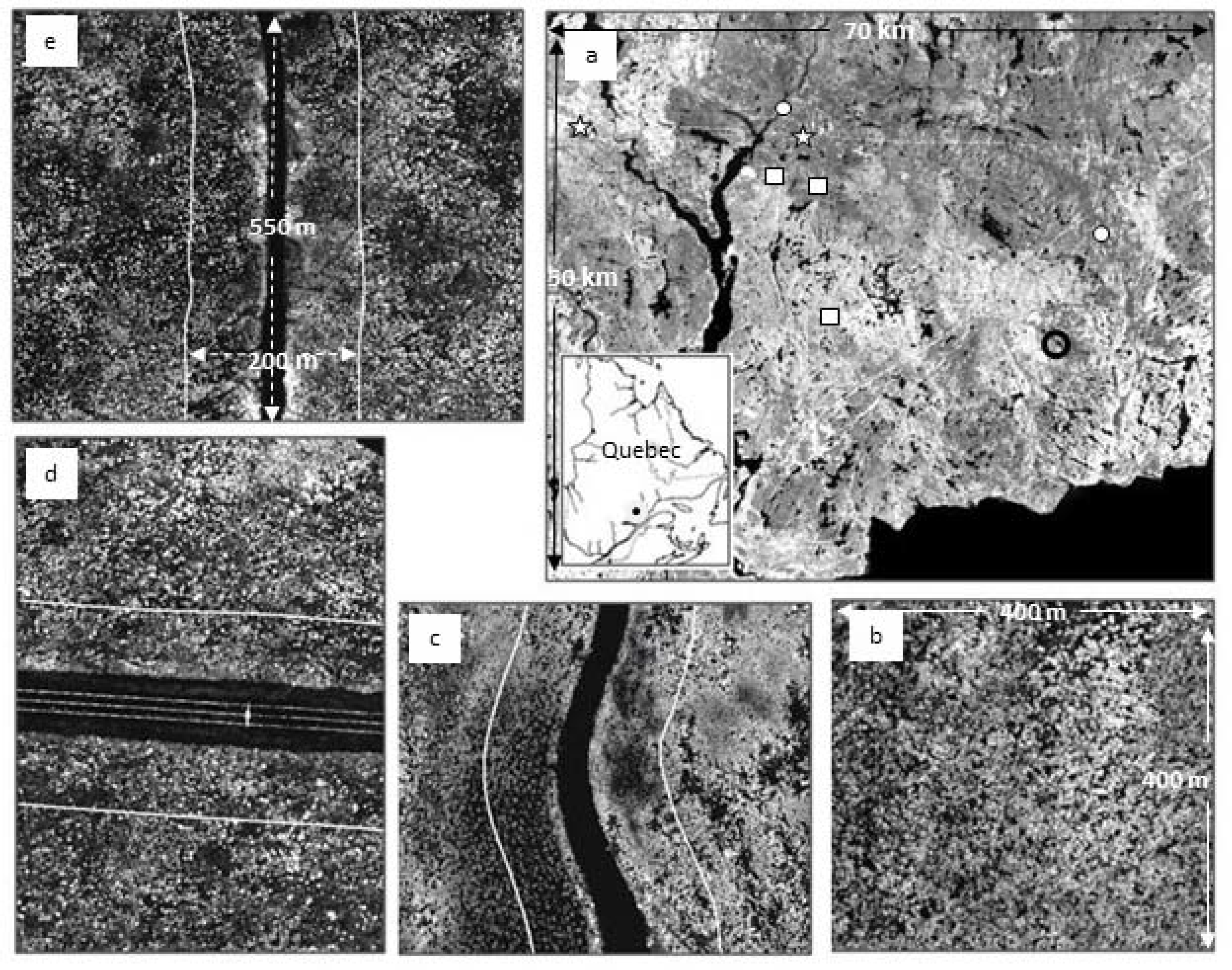
Figure 2.
Extraction of detailed forest structural variables in a large contiguous area using a LiDAR CHM. (a) A sample CHM of the road overlaid with 100 m buffer (two thick white lines) and 2 m buffer rings (thin white lines). (b) Enlarged window of the dotted line box of size 100 m × 100 m indicated on (a) showing automatically delineated individual stems. (c) Window of the dotted box indicated on (a) showing automatically delineated canopy gaps (hashed polygons). CHM is a canopy height model, and increase in height is given by progressively lighter shades in all figures.
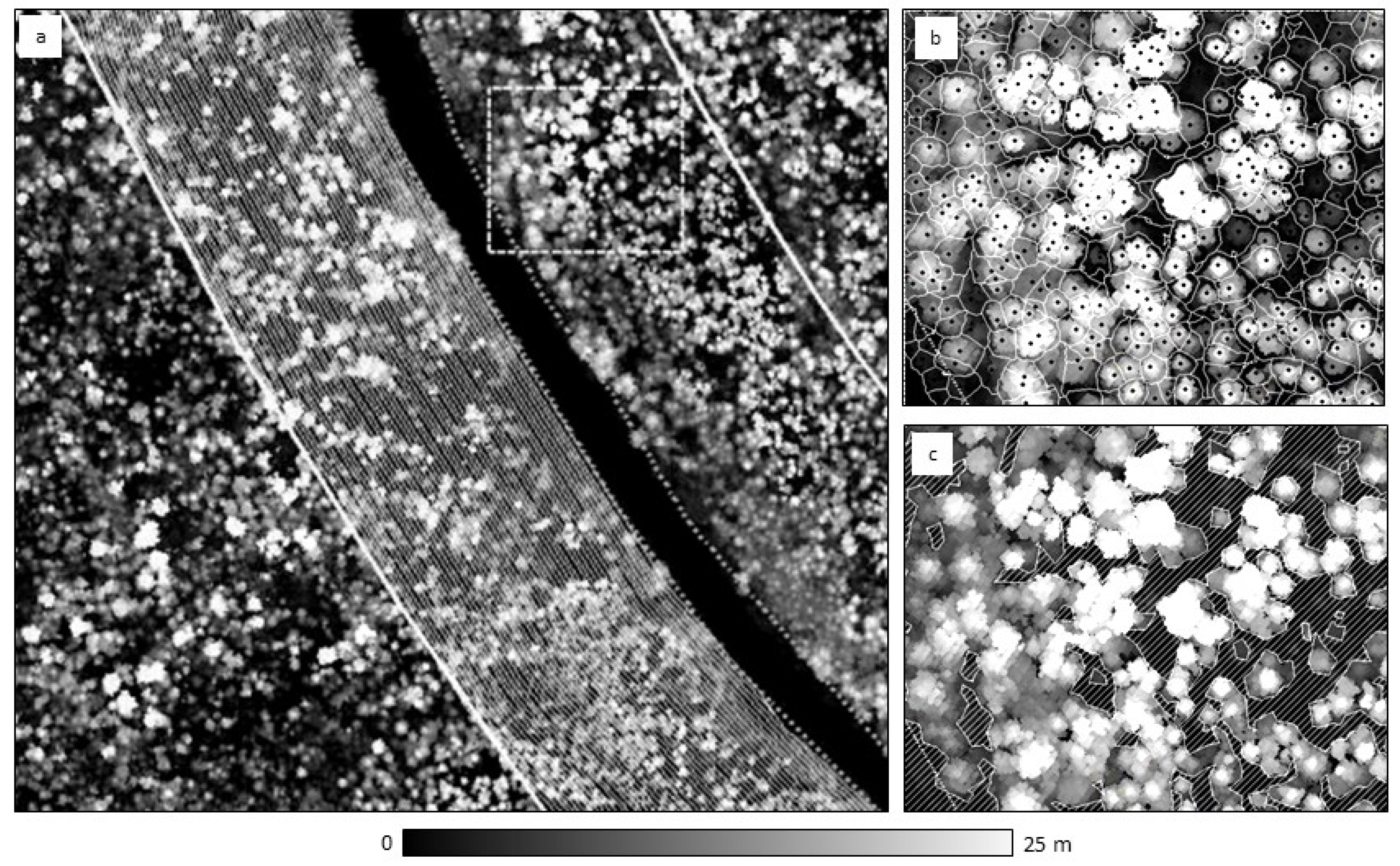
Figure 3.
Comparison of the frequency distribution of total height of individual trees in forests surrounding different linear openings with that of the undisturbed reference forest. Height distributions (a) for natural vs. anthropogenic openings, (b) between types of linear openings, (c) on both sides of natural linear openings oriented N-S, (d) on both sides of anthropogenic linear openings oriented N-S, and (e) on both sides of natural linear openings oriented E-W.

Figure 4.
Mean values of the response variables (listed in the heading of each column) with distance from the edge of a linear opening; (a–e) when compared to the reference forest; (f–j) between the types of linear openings. The dashed lines indicate the critical values of the response variables determined by bootstrap sampling for the reference forest. Significant values are those that occur outside the critical band.

Figure 5.
Magnitude of edge influence (MEI) for the response variables in different linear openings computed based on comparison with (a) reference forest; (b) natural openings. X-axis shows the MEI of each variable.
Figure 5.
Magnitude of edge influence (MEI) for the response variables in different linear openings computed based on comparison with (a) reference forest; (b) natural openings. X-axis shows the MEI of each variable.
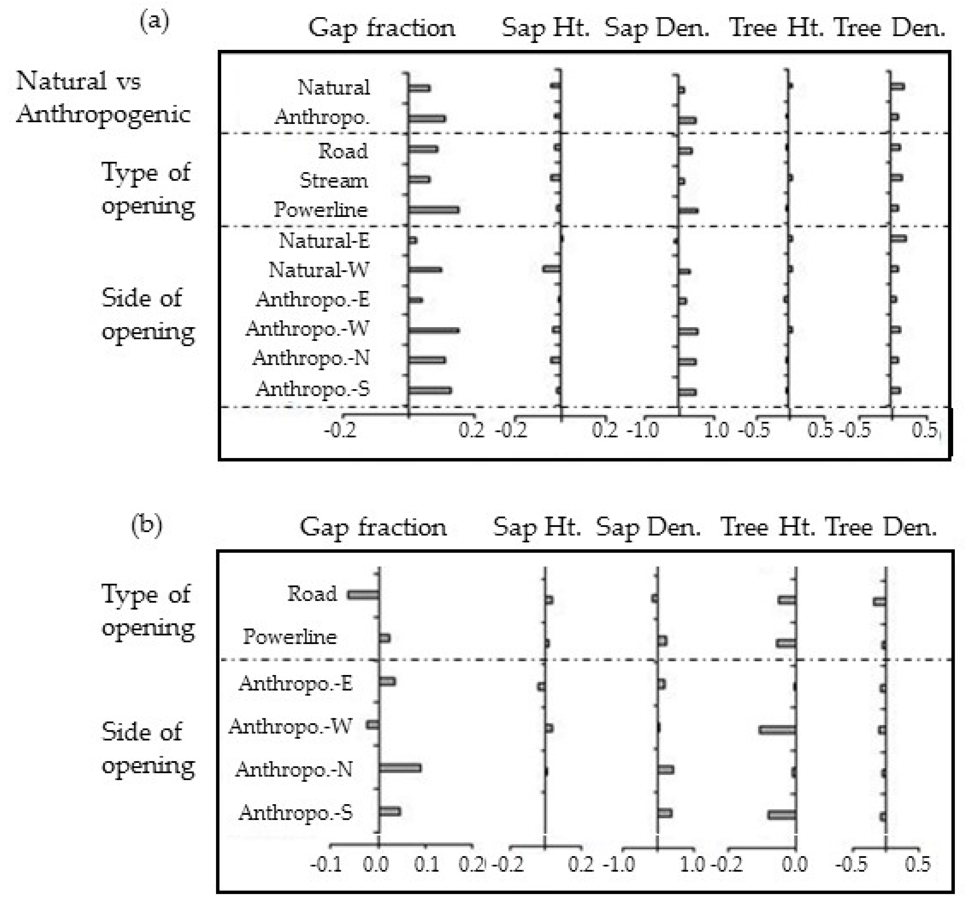
Figure 6.
Depth of influence (DEI) of selected linear openings on the adjoining forest due to the natural and anthropogenic linear openings, shown by cumulative average (CUAVG) curves of response variables against the distance from the edge of a linear opening. (a–e) Are the DEI of natural and anthropogenic openings; (f–j) are the DEI of the types of linear openings.

Table 1.
General characteristics of the selected linear openings.
| Type | Sampled Area | Width (m) | Orientation (°) | Length (m) | Total Area Sampled (ha) | Mean Elevation (m) | |
|---|---|---|---|---|---|---|---|
| Side 1 * | Side 2 * | ||||||
| Stream | 1 | 50 | 0 | 550 | 11 | 107 (E) | 105 (W) |
| 2 | 70 | 0 | 500 | 10 | 107 (E) | 106 (W) | |
| Road | 1 | 20 | 0 | 530 | 10.6 | 293 (E) | 288 (W) |
| 2 | 20 | 25 | 1200 | 24 | 242 (E) | 238 (W) | |
| 3 | 20 | 35 | 1000 | 20 | 380 (N) | 376 (S) | |
| Powerline | 1 | 90 | 270 | 530 | 10.6 | 330 (N) | 340 (S) |
| 2 | 150 | 325 | 1000 | 20 | 376 (N) | 380 (S) | |
* Two segments of the forest adjoining the opening e.g., an opening running in the east-west direction divides the forest into northern (N) and southern (S) segments. Mean elevation in the reference forest is 235 m.
Table 2.
Comparison of general characteristics of the forest conditions surrounding the selected linear openings (up to 100 m from the edge).
Table 2.
Comparison of general characteristics of the forest conditions surrounding the selected linear openings (up to 100 m from the edge).
| Comparison | Type | Gap Fraction | Sapling Height (m) | Sap. Density (stems/ha) | Tree Height (m) | Tree Density (stems/ha) | ||
|---|---|---|---|---|---|---|---|---|
| Mean | Max | Mean | Mean | Max | Mean | Mean | ||
| Natural vs. Anthropogenic | Natural | 0.41 ± 0.07 | 4.0 | 2.6 ± 0.5 | 46 ± 27 | 31.3 | 13.1 ± 0.4 | 746.6 ± 51.4 |
| Anthropo. | 0.45 ± 0.04 | 4.0 | 2.7 ± 0.1 | 93 ± 20 | 32.5 | 11.4 ± 0.3 | 659.9 ± 35.4 | |
| Nat. vs. Anth. | p < 0.01 | p < 0.05 | p < 0.05 | p < 0.05 | p < 0.05 | |||
| All features | Reference | 0.36 | 3.9 | 2.8 ± 0.8 | 32 | 25.6 | 11.9 ± 2.2 | 520 |
| Road | 0.43 ± 0.42 | 4.0 | 2.6 ± 0.1 | 77 ± 19 | 32.5 | 11.8 ± 0.4 | 663.6 ± 31.8 | |
| Stream | 0.41 ± 0.07 | 4.0 | 2.6 ± 0.5 | 46 ± 27 | 31.3 | 13.1 ± 0.4 | 746.6 ± 51.4 | |
| Powerline | 0.49 ± 0.43 | 4.0 | 2.7 ± 0.1 | 116 ± 33 | 31.3 | 10.8 ± 0.4 | 654.3 ± 56.0 | |
| Reference vs. linear openings | Ref. vs. all types | p < 0.01 | p < 0.01 | ns | ns | p < 0.001 | ||
| Ref. vs. type | p < 0.01 | p < 0.05 | p < 0.01 | ns | p < 0.001 | |||
| Natural vs. Anthropogenic vs. orientation | Natural-E | 0.38 ± 0.06 | 4.0 | 2.8 ± 0.3 | 25 ± 15 | 31.3 | 13.2 ± 0.6 | 830.2 ± 78.7 |
| Natural-W | 0.44 ± 0.09 | 4.0 | 2.4 ± 0.4 | 66 ± 40 | 29.8 | 13.1 ± 0.9 | 663.2 ± 75.2 | |
| Nat. E vs. W | p < 0.001 | p < 0.001 | p < 0.001 | ns | p < 0.001 | |||
| Anthropo.-E | 0.39 ± 0.05 | 4.0 | 2.7 ± 0.2 | 49 ± 27 | 26.8 | 10.6 ± 0.5 | 604.2 ± 45.5 | |
| Anthropo.-W | 0.49 ± 0.1 | 4.0 | 2.6 ± 0.2 | 118 ± 45 | 32.5 | 12.9 ± 0.7 | 679.8 ± 70.7 | |
| Nat. vs. Anth.-E | p < 0.05 | p < 0.001 | p < 0.01 | ns | p < 0.001 | |||
| Nat. vs. Anth.-W | p < 0.05 | ns | p < 0.01 | p < 0.001 | p < 0.001 | |||
| Anthropo.-N | 0.45 ± 0.03 | 4.0 | 2.6 ± 0.2 | 98 ± 28 | 31.1 | 11.2 ± 0.4 | 649.5 ± 50.3 | |
| Anthropo.-S | 0.47 ± 0.03 | 4.0 | 2.7 ± 0.2 | 100 ± 25 | 31.3 | 11.0 ± 0.4 | 694.2 ± 42.7 | |
Max: Maximum; Mean: Mean values (±1 SD); comparisons of distributions between two samples were made using Kolmogorov–Smirnov and Mann–Whitney U tests and, between multiple samples using Kruskal–Wallis 1-way. Nat.: Natural openings; Anth. Or Anthropo.: Anthropogenic openings; E: East; W: West; N: North; S:South; Ref: Reference forest; ns: non-significant.
© 2018 by the authors. Licensee MDPI, Basel, Switzerland. This article is an open access article distributed under the terms and conditions of the Creative Commons Attribution (CC BY) license (http://creativecommons.org/licenses/by/4.0/).
Share and Cite
MDPI and ACS Style
Vepakomma, U.; Kneeshaw, D.D.; De Grandpré, L. Influence of Natural and Anthropogenic Linear Canopy Openings on Forest Structural Patterns Investigated Using LiDAR. Forests 2018, 9, 540. https://doi.org/10.3390/f9090540
AMA Style
Vepakomma U, Kneeshaw DD, De Grandpré L. Influence of Natural and Anthropogenic Linear Canopy Openings on Forest Structural Patterns Investigated Using LiDAR. Forests. 2018; 9(9):540. https://doi.org/10.3390/f9090540
Chicago/Turabian StyleVepakomma, Udayalakshmi, Daniel D. Kneeshaw, and Louis De Grandpré. 2018. "Influence of Natural and Anthropogenic Linear Canopy Openings on Forest Structural Patterns Investigated Using LiDAR" Forests 9, no. 9: 540. https://doi.org/10.3390/f9090540
Note that from the first issue of 2016, this journal uses article numbers instead of page numbers. See further details here.