Biomass Modeling of Larch (Larix spp.) Plantations in China Based on the Mixed Model, Dummy Variable Model, and Bayesian Hierarchical Model


1
Key Laboratory of Tree Breeding and Cultivation of the State Forestry Administration, Research Institute of Forestry, Chinese Academy of Forestry, Dongxiaofu 1, Xiangshan Road, Haidian District, Beijing 100091, China
2
School of Forestry & Landscape of Architecture, Anhui Agricultural University, Hefei 230036, China
*
Author to whom correspondence should be addressed.
†
These authors contributed equally to this work.
Forests 2017, 8(8), 268; https://doi.org/10.3390/f8080268
Submission received: 8 May 2017
/
Revised: 16 July 2017
/
Accepted: 27 July 2017
/
Published: 27 July 2017
Abstract
:With the development of national-scale forest biomass monitoring work, accurate estimation of forest biomass on a large scale is becoming an important research topic in forestry. In this study, the stem wood, branches, stem bark, needles, roots and total biomass models for larch were developed at the regional level, using a general allometric equation, a dummy variable model, a mixed effects model, and a Bayesian hierarchical model, to select the most effective method for predicting large-scale forest biomass. Results showed total biomass of trees with the same diameter gradually decreased from southern to northern regions in China, except in the Hebei province. We found that the stem wood, branch, stem bark, needle, root, and total biomass model relationships were statistically significant (p-values < 0.01) for the general allometric equation, linear mixed model, dummy variable model, and Bayesian hierarchical model, but the linear mixed, dummy variable, and Bayesian hierarchical models showed better performance than the general allometric equation. An F-test also showed significant differences between the models. The R2 average values of the linear mixed model, dummy variable model, and Bayesian hierarchical model were higher than those of the general allometric equation by 0.007, 0.018, 0.015, 0.004, 0.09, and 0.117 for the total tree, root, stem wood, stem bark, branch, and needle models respectively. However, there were no significant differences between the linear mixed model, dummy variable model, and Bayesian hierarchical model. When the number of categories was increased, the linear mixed model and Bayesian hierarchical model were more flexible and applicable than the dummy variable model for the construction of regional biomass models.
1. Introduction
Forest biomass plays an important role in regulating global carbon balance to help mitigate the effects of climate change. With the development of large regional-scale biomass monitoring work, developing a biomass model for large-scale application has become an important job. In recent years, many researchers have explored biomass models at national, regional, and global levels [1,2,3,4]. Allometric equations were often used to estimate forest biomass in these studies [1,5,6,7,8]. The allometric equations usually had good fit performance and high values of R2, and the variables for prediction of aboveground biomass, such as tree diameter and height, are easy to measure in the field. However, a main drawback of these equations is that they produce different results when applied to sites outside the geographic allocation where the equations were originally developed [6,9,10]. Several authors have noted that the problem with the scaling coefficient in allometric equations is variation, which is dependent on species, tree stage, and site [7,9,11,12,13]. Case and Hall [3] also found that there was an increase in prediction error when using allometric equations to estimate tree biomass at different geographical scales. The crucial problem is how to make biomass models have a wider range of applicability, and not only meet the accuracy requirements for large-scale biomass estimates, but also improve local biomass prediction accuracy. The three models for estimating forest biomass, including the dummy variable model, the mixed effects model, and the Bayesian hierarchical model, provide possible solutions to this problem.
The mixed effects model is an improvement on the practical statistical techniques when estimating fixed effect and random effect parameters to reflect the difference between tree and plot, and to improve the precision of the prediction model [14]. In recent years, the mixed effects model has been widely used in the field of forestry. Fang and Bailey [15] applied a modified Richards growth function with nonlinear mixed effects for modeling slash pine dominant height growth with different silvicultural treatments. Daniel and Michael [16] developed a multilevel nonlinear mixed effects model system for describing dominant height, basal area, stand density, and volume. Zhang and Borders [17] used the mixed effects model to improve the precision of tree biomass estimation in the intensively managed loblolly pine plantations. Trincado and Burkhart (2006) [18] explored a nonlinear mixed effects model to describe stem taper, which showed that the method increased their prediction flexibility and efficiency. Fehrmann et al. [19] compared the mixed model with k-nearest neighbor methods in the establishment of Norway spruce and Scots pine tree biomass models in Finland. The relative root mean square errors of linear mixed models and k-nearest neighbor methods estimates are slightly lower than those of an ordinary least squares regression model. The results show that nonparametric methods are suitable in the context of single-tree biomass estimation. Derek et al. [20] applied the mixed effects model to develop branch models for white spruce with hierarchical structure data. In short, mixed effects models have become important tools for modeling tree height, stem taper, branch diameter, crown, and tree biomass. The Bayesian method is usually used to evaluate ecological models [4,21]. The results of Bayesian analyses with non-informative priors were similar to using parameters and statistics to fit allometric biomass equations with a classic statistical approach, however, the Bayesian method with informative priors performed better than the non-informative priors and the classic statistical approach [22,23,24,25]. In recent years, the Bayesian method has been widely used in forestry, for applications such as diameter distribution [26,27], tree growth [28], individual tree mortality [29,30], and stand-level height and volume growth models [11]. Zapata-Cuartas et al. [31] used Bayesian methods to estimate aboveground tree biomass, and obtained a reliable result. Zhang et al. [25] applied Bayesian methods to estimate Chinese fir tree biomass. When Bayesian methods are applied to quantify the forest biomass of a geographical location, the problems that occur often involve variation between different locations, which instead quantifies the hierarchical characteristics of the source data. The Bayesian hierarchical approach can resolve the problems in fitting the data. Zapata-Cuartas et al. [31] also concluded that the Bayesian hierarchical model may be an effective approach to improve biological estimation at a large regional scale.
In regression analysis, the dummy variable was considered as a virtual variable, which usually takes the values 0 or one [32]. The dummy variable method is commonly used to deal with indicator or categorical variables, which are involved in all quantitative methods (Tang et al., 2008; Fu et al., 2012) [33,34]. When the generalized model for a large-scale range is established, the dummy variable model is also a reliable model. Wang et al. [35] applied the mixed effects model and the dummy variable method to establish the dominant height model, and concluded that the two methods could be used to establish a specific parameter and obtained similar results. Fu et al. [34] used the linear mixed effects model and the dummy variable model to construct compatible single-tree biomass equations at different scales for Masson pine (Pinus massoniana) in southern China, and found that there were no significant differences between the results obtained from the two models.
Larch (Larix spp.), a fast-growing deciduous coniferous tree, is one of the main tree species used for timber production in China. Because it has a straight stem, better quality timber, and high commercial value, the planting area and volume for larch plantations in China are approximately 3.14 million ha, 18.4 million m3, respectively [36]. Currently, the larch plantations, not only provide a large volume of commercial timber, but also play an important role in forest carbon fixation. Therefore, the goal of this research was to build larch stem wood, branches, stem bark, needle, root, and total biomass models at the regional level, using a general allometric equation, the dummy variable model, the mixed effects model, and the Bayesian hierarchical model, to select the most effective method for predicting large-scale tree biomass.
2. Materials and Methods
2.1. Site Description
2.2. Biomass Data
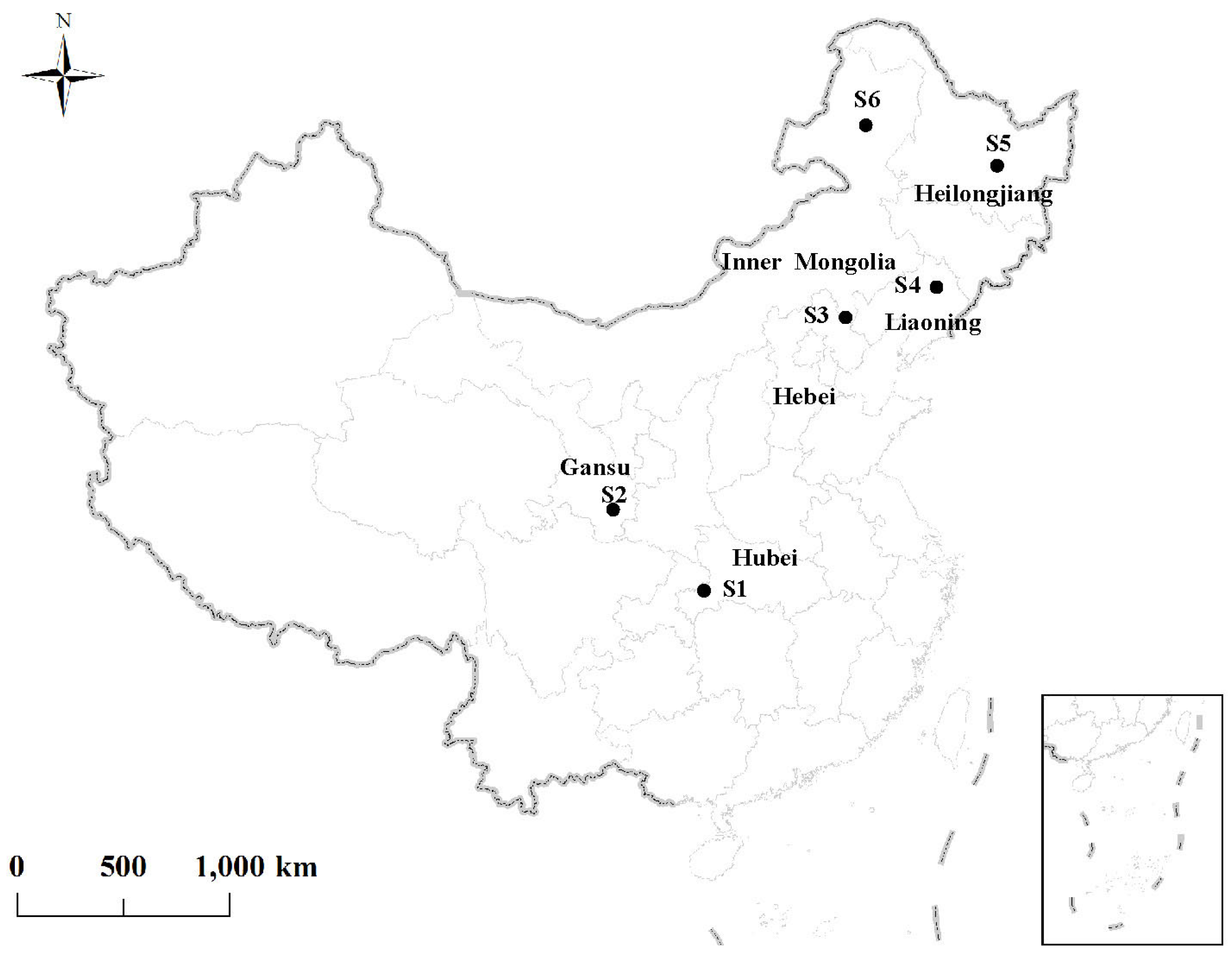
The biomass data of 360 sample trees from 209 plots were used in this study, which were collected via destructive sampling from Larch plantations in China between 2009 and 2013. The sample plots were located in Hubei, Gansu, Hebei, Liaoning, and Heilongjiang provinces and the Inner Mongolia autonomous region (Figure 1). The data covered the complete period of stand development for timber production, with stand age ranging from 3 to 45 years. The stem diameter at breast height (DBH), total height (HT), height to crown base (HCB), and crown width (CW) were recorded for each tree within the plots. The sample trees were chosen according to the dominant, average, and inferior tree outside the plot in the stand. Then the sample trees were felled as carefully as possible to minimize damage to their crowns. The tree height, live crown length, and height of lowest living branch of the trees were recorded, and subsequently the trees were stripped of their branches. The live crown was divided into three parts: top, middle, and bottom. From each part, two branches were selected for further sub-sampling in order to determine fresh and oven-dried biomass ratio. For about half of the sub-samples, shoots were further sub-sampled by removing all needles from the branches in order to determine needle to branch biomass ratio. All of the branches were removed and the tree length was recorded. Each stem was then divided into 1m sections. The fresh weight of each stem section was measured. From each section, a stem disc (2 cm wide) was taken as a sub-sample in order to determine the fresh to oven-dried biomass ratio for each stem section. The bark of each stem disc was removed and the bark to wood mass ratio was determined in the lab. The whole roots were manually excavated, and were then sorted into root stump, large roots (≥5 cm), medium roots (2–5 cm) and small roots (≤2 cm). The aboveground stumps that remained after tree felling were included in the root stump biomass. The fresh biomass of each root diameter class was determined in the field. Sub-samples of each class were taken and their fresh biomass was determined with an electronic balance. All sub-samples of branches, needles, stem wood, stem bark, and roots were oven-dried at 80 °C until a constant weight was reached (usually within 24–48 h). According to the ratios of fresh to oven-dried biomass, the total branch, needle, stem wood, stem bark, and root biomass were calculated. The biomass data of each component in different regions was summarized in Table 2.
2.3. Statistical Analysis
2.3.1. General Model
Allometric equations were widely used for estimating biomass [1,2,5,7]. The form of the equation provides a good balance between accurate predictions and low data requirements by using the most commonly and easily measured variable, which is DBH. We also used the following allometric equation as a base model to construct different biomass equations in this study:
where Y is the oven-dry weight of the biomass component of a tree, DBH is the diameter at breast height in cm, δ represents the multiplicative error term, and a and b are parameters.
Equation (1) can be changed into the following linear form by logarithmic transformation:
where: y = lnY, x = lnDBH, a0 = lna, .
2.3.2. Dummy Variable Model
The general form of the dummy variable model based on Equation (2) is expressed as follows:
where zi is the dummy variable, ai is the corresponding specific parameter of region i, other parameters are the same as in Equation (2).
2.3.3. Linear Mixed Effects Model
The general form of the linear mixed effects model is as follows [14,32,33]:
where is the ni-dimensional response vector for the ith region; β is the p-dimensional parameter vector for fixed-effects; is the ni × p design matrix for fixed-effects variables; ui is the q-dimensional region-specific vector of parameters for random effects (only one random effect); Zi is the ni × q design matrix for random-effect variables (random effect of the ith region); is the ni-dimensional error vector. It is assumed that: , , , . Further, it is common to assume that and are normally distributed and thus: and .
2.3.4. Bayesian Hierarchical Model
Equation (2) could be changed into the following form when the Bayesian hierarchical approach is used:
where , are cluster-specific random variables to be predicted and assumed to be , and , respectively. is assumed to be . Variance, or , measures the between-subject variability, while accounts for the within-subject variability for all the regions.
The relevant prior knowledge about the data can be incorporated into Bayesian analyses, which contrast the classical statistical approach [37]. In the study, we need to choose appropriate prior distributions for all parameters, including a and b. The prior distributions of a and b (total tree, root, stem wood, stem bark, branch, and needle) were obtained for 36 biomass equations from six Chinese larch publications (Appendix Table A1) [38,39,40,41,42,43]. We assume the parameters a and b are distributed as a bivariate normal distribution. The Bayesian hierarchical model was fitted using the MCMC method in the R package R2WinBUGS [44].
2.3.5. Model Fitting and Evaluating
The general model, dummy variable model, linear mixed model, and Bayesian hierarchical approach were used to establish the stem wood, stem bark, branch, needle, root, and total biomass models. All the models were fitted using the “R3.2.1” software. The following statistics were calculated to compare the effect of the region-level biomass for larch plantations: prediction determination coefficient (R2), root mean square error (RMSE), and absolute bias (MAB).
where is the observed biomass values, is the arithmetic mean of all observed biomass values, is the estimated biomass values based on models, and n is the sample number.
3. Results
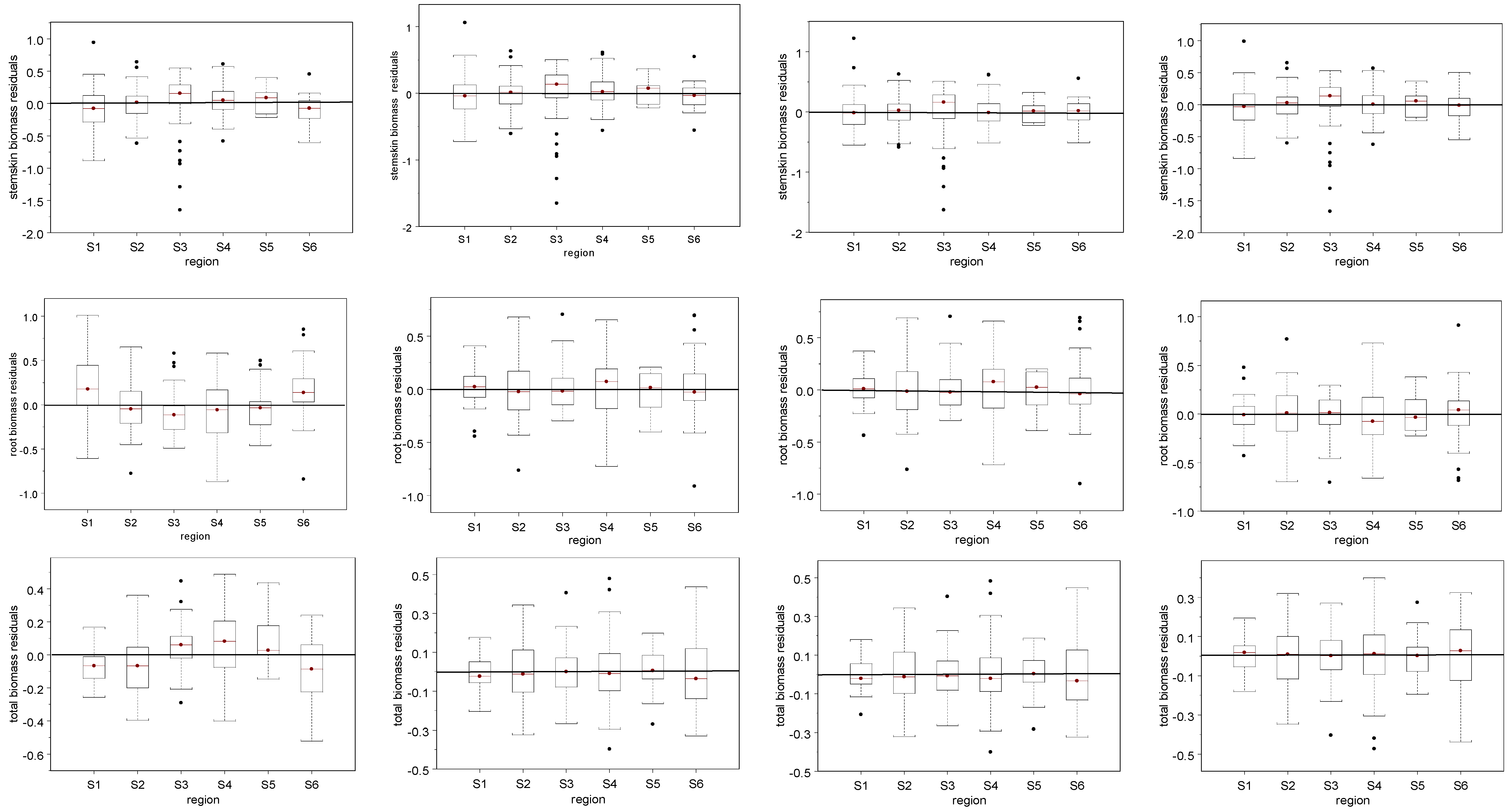
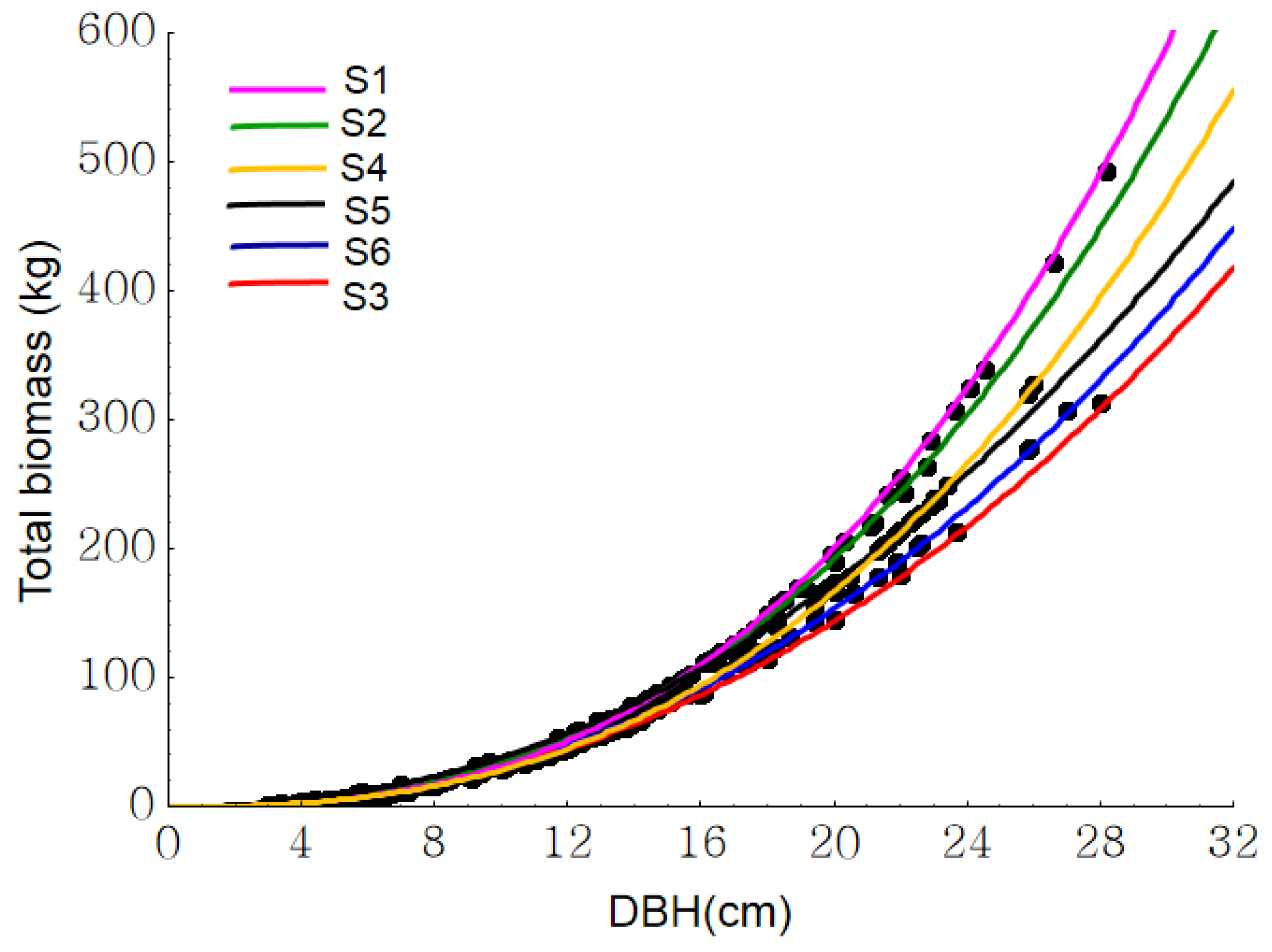
In this study, the general biomass model, Equation (2), the dummy variable model, Equation (3), linear mixed effects model, Equation (4), and the Bayesian hierarchical model, Equation (5), were used to fit the biomass data on 360 sample larch trees from six regions (S1, S2, S3, S4, S5, S6) in China, developing the model of total tree, root, stem wood, stem bark, branch, and needle biomass respectively. Parameter estimates of the models, Equations (2)–(5) are presented in Table 3, Table 4, Table 5 and Table 6. The parameters of each model were statistically significant (p < 0.01), and the parameters of the dummy variable model, linear mixed effects model, and Bayesian hierarchical model may predict the biomass of different regions. The residual distributions of the dummy variable model, linear mixed effects model, and Bayesian hierarchical model were better than the general biomass model, and they were more uniform and had no obvious residual trends (Figure 2). The special and random parameters of region type indicate that the biomass component of a tree in six regions are obviously different. In addition, the biomass of a tree with the same diameter gradually decreased from southern to northern regions in China, except in region S3, Weichang County in Hebei Province, in a temperate region. However, the differences were not statistically significant. For example, when the tree diameter at breast height was 25 cm, the total biomass of single tree was 356 kg on the Changlinggang farm in Hubei (S1) in the northern subtropical region; 333 kg in Tianshui City in Gansu (S2) in the warm–temperate region; 293 kg on the Dagujia farm in Liaoning (S4) in a temperate region; 286 kg on the Mengjiagang farm in Heilongjiang (S5) and 256 kg in the Wuerqihan Forestry Bureau in the Inner Mongolia autonomous region (S6), which are both located in a cold–temperate region; and 239 kg in Hebei (S3) (Figure 3). In terms of the three fit statistics (R2, MAB and RMSE) for the general biomass model (Equation (2)), the dummy variable model (Equation (3)), the linear mixed effects model (Equation (4)) and the Bayesian hierarchical model (Equation (5)) are presented in Table 7. It was found that the R2 values of Equations (3)–(5) were larger than Equation (2), and MAB and RMSE were lower than Equation (2), when they were used to estimate stem wood, stem bark, branch, needle, root, and total biomass. This indicated that the dummy variable model, mixed effect model, and Bayesian hierarchical model were better in the prediction of biomass than the general biomass model. Additionally, the fitting optimization index of the F-test also verified the results (Table 7). However, there were no significant differences among the results of fitting for the mixed effect model, dummy variable model, and Bayesian hierarchical model. In other words, the accuracy of prediction of biomass using the mixed effects model, dummy variable model, and Bayesian hierarchical model were similar. For the three models, the Bayesian hierarchical model was slightly better for predicting stem wood biomass. The predicted results of the biomass component indicated that the generalized R2 is highest for stem wood, bark, root, total biomass, and lowest for needle and branch biomass. This may be due to the difficulties with available sample crown. In short, in this study, each component biomass model and total biomass model were well developed in different regions. Based on RMSE, MAB, and R2 values, it could be concluded that the mixed model, dummy variable model, and Bayesian hierarchical model performed better than the general model, and the results of the three methods were approximate in their ability to describing the fit of the data.
4. Discussion
Larch is one of the most important afforestation tree species in China. The accurate estimation of larch biomass and carbon stock is critical. Allometric equations have been widely used to estimate forest biomass in many studies, but the use of allometric equations in regions outside the area in which they were developed or for different species, has been strongly debated in forestry literature. Some authors have even recommended using general allometric equations [12,13]. In this study, the scaling coefficient in allometric equations was varied in different biomass components (stem wood, branches, stem bark, needle, root and total biomass), and across different larch species and regions. Although it is generally known that the scaling exponent b is between two and three [12], it is also usually realized as a species-specific equation, with different coefficients a and b, because trees may differ in architecture as well as wood density [6,45]. West et al. [46] applied a process-based model which is called the WBE model, to estimate values of scaling exponents using a functional relationship; it indicated that the aboveground biomass of a tree species should scale against stem diameter with b = 8/3 (2.67), regardless of species, site, and age. However, Zianis and Mencuccini [12] estimated another empirical exponent (b = 2.36) based on a worldwide list of 279 biomass allometric equations, which is different from the scaling exponent (b ≈ 2.67). They indicated that the ratio of biomass and DBH for trees growing in different environmental conditions cannot be constant. In the study, the average value of parameter b was 2.42 for the total biomass model, and it did not differ from the theoretical value (2.67) and empirical value (2.36), because the scaling exponent (b = 2.67 or 2.36) is the average of all species. For larch plantation, the b value (2.42) may be more appropriate.
The larch data was collected from the six main ecological regions in China for larch plantation distribution and growth. The biomass equations suitable for application to regional forest biomass prediction are the linear mixed model, dummy variable model, and Bayesian hierarchical model. Based on the three evaluation statistics (R2, RMSE, MAB), the four models were compared: the general biomass model (Equation (2)), the dummy variable model (Equation (3)), the linear mixed model (Equation (4)), and the Bayesian hierarchical model (Equation (5)). There were no significant differences among the three statistics of fit in the dummy variable model, linear mixed model, and Bayesian hierarchical model. However, when compared with the general biomass model, dummy variable model, linear mixed model, and Bayesian hierarchical were significantly better; F-test and residual plots also verified the significant differences.
Some studies only compared the dummy variable model with the mixed effect model in solving large-scale forestry biomass and growth estimation accuracy problems [34,35]. In this study, an alternative method, the Bayesian hierarchical model, was used to model the large-scale tree biomass. Bayesian inference has been developed in forest biomass estimates [25,31]. The main difference between Bayesian and classical approaches is how to define their prior knowledge of the sample data. The classical approach assumes the parameters are a fixed and unknown constant, whereas the Bayesian approach assumes that the parameters follow some statistical distribution, especially for a bivariate normal distribution [25,31]. Due to known prior data, the Bayesian method has advantages in the prediction of small sample data. Zapata-Cuartas et al. [31] built the biomass model using the Bayesian and the classical approach to compare model precision of different sample sizes of 6, 10, 20, 30, 40, 50 and 60, and found that model efficiency (RMSE) of two approaches was almost similar when the sample size was larger than 60, otherwise the Bayesian approach was superior. Huang et al. [47] also indicated that the fitted precision for tree biomass using the Bayesian approach was better than the classical approach when the sample size was smaller than 50. Thus, using the Bayesian method, with small sample data to estimate forest biomass will significantly reduce the time and costs of sampling. The emphasis of this study is mainly on methodology. Choosing between the dummy model and mixed model for prediction of forest biomass has been a hot research topic with the aim of improving the accuracy of models for application in large regional scales [34,35]. For practical applications, the choice of model depends on a number of categories (i.e., regions) and the sample number in each category. If the number of categories is small (less than 10), the dummy model is preferred; if the number of categories is large, the mixed model is more appropriate [35]. However, the Bayesian hierarchical method has advantages in the prediction of small sample data (numbers < 60) [31,47]. In this paper, we defined the categories by the six geographical regions, and the number of samples per region was equal to 60. Furthermore, the sample trees from each region came from various larch plantations which covered different site conditions, stand ages, and stand densities. Thus, it is necessary to analyze the random effects, taking the specific region’s variables as random parameters in the mixed model. Because the sample number is equal to 60, the effect of the Bayesian hierarchical model is the same as the linear mixed model. Based on this knowledge, we tend to recommend the mixed model and the Bayesian hierarchical model for developing larch stem wood, branch, stem bark, needle, root, and total biomass models.
The three methods (dummy variable model, linear mixed model, and Bayesian hierarchical model) have no differences in regional biomass estimation ability. The modeling results showed that the total biomass of a tree with the same diameter gradually decreased from the southern to northern regions in China, except in Hebei Province (S3) (Figure 3). This may be because the water and heat conditions in the southeastern region are better and the trees have enough growing space, but from south to north, the water and heat conditions worsen, which impacts the growth and development of the trees. In addition, the sample plots in Hebei Province (S3) were located in a plateau region with high winds, sandy soil, and limited recipitation. The climate conditions may have resulted in larch having the lowest biomass in this region (S3).
5. Conclusions
Based on the biomass data for larch plantations in China, the generalized single tree biomass model suitable for regional scale forest biomass estimation was developed using the dummy variable model, linear mixed model, and Bayesian hierarchical model, which solved the problem of forest biomass estimate accuracy amongst different geographical scales. Our results indicate that using the mixed model, dummy variable model, and Bayesian hierarchical model improved the model-fitting results, providing an effective method for estimating larch biomass at the regional scale. Note that if the model fitting process accounts for differences in species and origins as a nested factor based on regional differences, the model fitting results should improve, and the mixed model, dummy variable model, and Bayesian hierarchical model would be more effective than the general allometric equations. The choice of the dummy variable model, mixed model, or Bayesian hierarchical model mainly depends on number of categories and samples. If the number of categories is larger, the mixed model and Bayesian hierarchical model should be the better choices. When the sample numbers are less than 60, the Bayesian hierarchical model may be more appropriate. In general, the mixed model and Bayesian hierarchical model are more flexible and applicable. The modeling results showed that the total biomass of a tree with the same diameter gradually decreased from southern to northern regions in China, except in Hebei Province (S3).
Acknowledgements
We would like to thank the National Natural Science Foundation (No. 31430017 and No. 31300536) and Special Fund for Basic Scientific Research Business of Central Public Research Institutes (No. CAFYBB2014QB005) for financial support for this study.
Author Contributions
Conceived and designed the experiments: D.-S.C. and S.-G.Z. Performed the experiments: D.-S.C. and X.-Z.H. Analyzed the data: D.-S.C. Contributed reagents/materials/analysis tools: X.-M.S. and S.-G.Z. Wrote the paper: D.-S.C.
Conflicts of Interest
The authors declare no conflicts of interest.
Appendix

Table A1.
a and b values of 36 biomass equations(total, root, stem wood, stem bark, branch, and foliage biomass) in six reports for larch in China.
Table A1.
a and b values of 36 biomass equations(total, root, stem wood, stem bark, branch, and foliage biomass) in six reports for larch in China.
| No. | Total | Root | Stem wood | Stem Bark | Branch | Foliage | Reference | ||||||
|---|---|---|---|---|---|---|---|---|---|---|---|---|---|
| a | b | a | b | a | b | a | b | a | b | a | b | ||
| 1 | −1.378 | 0.760 | −0.929 | 0.368 | −2.957 | 0.911 | −4.962 | 0.913 | −1.448 | 0.307 | −4.017 | −1.378 | (Wang, 2010) [38] |
| 2 | −1.952 | 0.844 | −4.075 | 0.915 | −2.797 | 0.888 | −3.352 | 0.670 | −2.957 | 0.633 | −3.817 | −1.952 | (Shen et al, 2011) [39] |
| 3 | −2.087 | 0.892 | −4.510 | 0.981 | −2.465 | 0.849 | −3.381 | 0.684 | −4.423 | 0.990 | −5.521 | −2.087 | (Liu, 2012) [40] |
| 4 | −2.079 | 0.901 | −4.510 | 0.982 | −2.659 | 0.927 | −3.352 | 0.694 | −3.037 | 0.628 | −3.058 | −2.079 | (Zhang, 2010) [41] |
| 5 | −1.091 | 0.735 | −5.116 | 1.024 | −1.845 | 0.789 | −1.917 | 0.389 | −1.514 | 0.318 | −0.942 | −1.091 | (Min, 2010) [42] |
| 6 | −2.419 | 0.929 | −3.474 | 0.866 | −3.170 | 0.960 | −4.269 | 0.813 | −5.298 | 0.972 | −4.962 | −2.419 | (Li, 2013) [43] |
References
- Jenkins, J.C.; Chojnacky, D.C.; Heath, L.S.; Birdsey, R.A. National-scale biomass estimators for United States tree species. For. Sci. 2003, 49, 12–35. [Google Scholar]
- Muukkonen, P. Generalized allometric volume biomass equations for some tree species in Europe. Eur. J. For. Res. 2007, 126, 157–166. [Google Scholar] [CrossRef]
- Case, B.; Hall, R.J. Assessing prediction errors of generalized tree biomass and volume equations for the boreal forest region of west-central Canada. Can. J. For. Res. 2008, 38, 878–889. [Google Scholar] [CrossRef]
- Lydia, R.O.; Halloran, E.T.; Borer, E.W.; Seabloom, A.S.; MacDougall, E.E.; Cleland, R.L.; McCulley, S.H.; Hobbie, W.; StanHarploe, N.M.; DeCrappeo, J.D.; et al. Regional Contingencies in the relationship between aboveground biomass and litter in the world’s grasslands. PLoS ONE 2013, 8, 1–9. [Google Scholar] [CrossRef] [Green Version]
- Ter-Mikaelian, M.T.; Korzukhin, M.D. Biomass equations for sixty-five North American tree species. For. Ecol. Manag. 1997, 97, 1–24. [Google Scholar] [CrossRef]
- Zianis, D.; Muukkonen, P.; Makipaa, R.; Mencuccini, M. Biomass and stem volume equations for tree species in Europe. Silva Fenn. Monogr. 2005, 4, 1–63. [Google Scholar]
- Návar, J. Allometric equations for tree species and carbon stocks for forests of northwestern Mexico. For. Ecol. Manag. 2009, 257, 427–434. [Google Scholar] [CrossRef]
- Adriano, L.; Rempei, S.; Gabriel, H.P.M.R.; Takuya, K.J.; Joaquim, D.S.; Roseana, P.S.; Cacilda, A.S.S.; Priscila, C.B.; Hideyuki, N.; Moriyoshi, I.; et al. Allometric models for estimating above- and below-ground biomass in Amazonian forests at Sao Gabriel da Cachoeira in the upper Rio Negro. Brazil. For. Ecol. Manag. 2012, 277, 163–172. [Google Scholar]
- Clark, D.B.; Clark, D.A. Landscape-scale variation in forest structure and biomass in a tropical rain forest. For. Ecol. Manag. 2000, 137, 185–198. [Google Scholar] [CrossRef]
- Chambers, J.Q.; Santos, J.D.; Ribeiro, R.J.; Higuchi, N. Tree damage, allometric relationships, and above-ground net primary production in central Amazon forest. For. Ecol. Manag. 2001, 152, 73–84. [Google Scholar] [CrossRef]
- Li, R.; Stewart, B.; Weiskittel, A. A Bayesian approach for modeling nonlinear longitudinal/hierarchical data with random effects in forestry. Forestry 2012, 85, 17–25. [Google Scholar] [CrossRef]
- Zianis, D.; Mencuccini, M. On simplifying allometric analyses of forest biomass. For. Ecol. Manag. 2004, 187, 311–332. [Google Scholar] [CrossRef]
- Pilli, R.; Anfodillo, T.; Carrer, M. Towards a functional and simplified allometry for estimating forest biomass. For. Ecol. Manag. 2006, 237, 583–593. [Google Scholar] [CrossRef]
- Ramon, C.L.; George, A.M.; Walter, W.S.; Russell, D.W.; Oliver, S. SAS for Mixed Model, 2nd ed.; SAS Institute Inc.: Cary, NC, USA, 2006. [Google Scholar]
- Fang, Z.; Bailey, R.L. Nonlinear mixed effects modeling for Slash pine dominant height growth following intensive silvicultural treatments. For. Sci. 2001, 47, 287–300. [Google Scholar]
- Daniel, B.H.; Michael, C. Multivariate multilevel nonlinear mixed effects models for timber yield predictions. Biometrics 2004, 60, 16–24. [Google Scholar]
- Zhang, Y.J.; Borders, B.E. Using a system mixed effects modeling method to estimate tree compartment biomass for intensively managed loblolly pines-an allometric approach. For. Ecol. Manag. 2004, 194, 145–157. [Google Scholar] [CrossRef]
- Trincado, G.; Burkhart, H.E. A generalized approach for modeling and localizing stem profile curves. For. Sci. 2006, 52, 670–682. [Google Scholar]
- Fehrmann, L.; Lehtonen, A.; Kleinn, C.; Tomppo, R. Comparison of linear and mixed-effect regression models and a k-nearest neighbor approach for estimation of singletree biomass. Can. J. For. Res. 2008, 38, 1–9. [Google Scholar] [CrossRef]
- Derek, F.S.; Philip, G.C.; Alexis, A. Branch models for white spruce (Piceaglauca. (Moench.) Voss) in naturally regenerated stands. For. Ecol. Manag. 2014, 325, 74–89. [Google Scholar]
- Anholt, B.R.; Werner, E.; Skelly, D.K. Effect of food and predators on the activity of four larval ranid frogs. Ecology 2000, 81, 3509–3521. [Google Scholar] [CrossRef]
- Berger, J.; Berry, D.A. Statistical analysis and the illusion of objectivity. Am. Sci. 1988, 76, 159–165. [Google Scholar]
- Jaynes, E.T. Probability Theory: The Logic of Science; Cambridge University Press: New York, NY, USA, 2003; pp. 19–55. [Google Scholar]
- Ellison, A.M. Bayesian inference in ecology. Ecol. Lett. 2004, 7, 509–520. [Google Scholar] [CrossRef]
- Zhang, X.Q.; Duan, A.G.; Zhang, J.G. Tree Biomass Estimation of Chinese fir (Cunninghamialanceolata.) based on Bayesian method. PLoS ONE 2013, 8, 1–11. [Google Scholar] [CrossRef]
- Bullock, B.P.; Boone, E.L. Deriving tree diameter distributions using Bayesian model averaging. For. Ecol. Manag. 2007, 242, 127–132. [Google Scholar] [CrossRef]
- Green, E.J.; Roesch, F.A.; Smith, F.M.; Strawderman, W.E. Bayesian estimation for the three-parameter Weibull distribution with tree diameter data. Biometrics 1994, 50, 254–269. [Google Scholar] [CrossRef]
- Clark, J.S.; Wolosin, M.; Dietze, M.; Ibanez, I.; Ladeau, S.; Welsh, M.; Kloeppel, B. Tree growth inference and prediction from diameter censuses and ring widths. Ecol. Appl. 2007, 17, 1942–1953. [Google Scholar] [CrossRef] [PubMed]
- Metcalf, C.J.E.; McMahon, S.M.; Clark, J.S. Overcoming data sparseness and parametric constraints in modeling of tree mortality: A new nonparametric Bayesian model. Can. J. For. Res. 2009, 39, 1677–1687. [Google Scholar] [CrossRef]
- Zhang, X.Q.; Zhang, J.G.; Duan, A.G. A hierarchical Bayesian model to predict self-thinning line for Chinese Fir in Southern China. PLoS ONE 2015, 10, 1–11. [Google Scholar] [CrossRef] [PubMed]
- Zapata-Cuartas, M.; Sierra, C.A.; Alleman, L. Probability distribution of allometric coefficients and Bayesian estimation of aboveground tree biomass. For. Ecol. Manag. 2012, 277, 173–179. [Google Scholar] [CrossRef]
- Tang, S.Z.; Li, Y. Statistical Foundation for Biomathematical Models; Science Press: Beijing, China, 2002; pp. 168–194. (In Chinese) [Google Scholar]
- Tang, S.Z.; Lang, K.J.; Li, H.K. Statistics and Computation of Biomathematical Models (For Stat Course); Science Press: Beijing, China, 2008; pp. 115–261. (In Chinese) [Google Scholar]
- Fu, L.Y.; Zeng, W.S.; Tang, S.Z.; Sharma, R.P.; Li, H.K. Using linear mixed model and dummy variable model approaches to construct compatible single tree biomass equations at different scales—A case study for Masson pine in Southern China. J. For. Sci. 2012, 58, 101–115. [Google Scholar]
- Wang, M.; Borders, B.E.; Zhao, D. An empirical comparison of two subject-specific approaches to dominant heights modeling, the dummy variable method and the mixed model method. For. Ecol. Manag. 2008, 255, 2659–2669. [Google Scholar] [CrossRef]
- China Forestry Bureau. The Eighth Forest Resource Survey Report; Chinese Forestry Press: Beijing, China, 2014; p. 18. (In Chinese)
- Wagner, H.; Tüchler, R. Bayesian estimation of random effects models for multivariate responses of mixed data. Comput. Stat. Data Anal. 2010, 54, 1206–1218. [Google Scholar] [CrossRef]
- Wang, H.Q. Research on the Biomass Model of Larix kaemferi Plantation in Northern Sub-Tropical Alpine area Based on Sample Plots and Remote Sensing. Master of Thesis, Chinese Academy of Forestry, Beijing, China, 2010; Science Press, Beijing, China, 2008. [Google Scholar]
- Shen, Y.Z.; Sun, X.M.; Zhang, J.T.; Du, Y.C.; Ma, J.W. Study on the individual tree biomass of Larix kaempferi plantation in Xiaolong mountain Gansu province. For. Res. 2011, 24, 517–522. (In Chinese) [Google Scholar]
- Liu, Y.Q. The Study of Single Biomass, Carbon Storage and Distribution of Larixprincipis-rupprechtii and Populus in Hebei Province. Master of Thesis, Agricultural University of Hebei, Baoding, China, 2012. (In Chinese). [Google Scholar]
- Zhang, H. Study on the Dominant Tree Biomass and Carbon Storage in Daqing Mountain. Master of Thesis, Inner Mongolia Agricultural University, Huhehaote, China, 2010. (In Chinese). [Google Scholar]
- Min, Z.Q. Study on Biomass Estimation Model of Larix olgensis. Master of Thesis, Beijing Forestry University, Beijing, China, 2010. (In Chinese). [Google Scholar]
- Li, Z.F. Biomass and Carbon Storage of the Larix gmelinii Forest’s Research. Master of Thesis, Inner Mongolia Agricultural University, Huhehaote, China, 2013. (In Chinese). [Google Scholar]
- Sturtz, S.; Ligges, U.; Gelman, A. R2WinBUGS: A package for running WinBUGS from R.J. Stat. Softw. 2005, 12, 1–16. [Google Scholar]
- Ketterings, Q.A.; Coe, R.; Van Noordwijk, M.; Ambagau, Y.; Palm, C.A. Reducing uncertainty in the use of allometric biomass equations for predicting above-ground tree biomass in mixed secondary forests. For. Ecol. Manag. 2001, 146, 199–209. [Google Scholar] [CrossRef]
- West, G.B.; Brown, J.H.; Enquist, B.J. A general model for the structure and allometry of plant vascular systems. Nature 1999, 400, 664–667. [Google Scholar]
- Huang, X.Z.; Chen, D.S.; Sun, X.M.; Zhang, S.G. Estimation of above-ground tree biomass based on probability distribution of allometric parameters. Sci. Silvae Sin. 2014, 50, 34–41. (In Chinese) [Google Scholar]
Figure 1.
The regions where the stem wood, branch, needle, stem bark, root, and total biomass data were collected. Black dots represent specific locations for data collection, S1 in Hubei Province (30°48′ N, 110°02′ E), S2 in Gansu Province (34°09′ N, 105°52′ E). S3 in Hebei Province (41°43′ N, 118°7′ E). S4 in Liaoning Province (42°21′ N, 124°52′ E). S5 in Heilongjiang Province (46°32′ N, 129°10′ E). S6 in Inner Mongolia (49°34′ N, 121°25′ E).

Figure 2.
Residual boxplots of the biomass component of all models (A–D) represent the general biomass model, linear mixed effects model, the dummy variable model, and the Bayesian hierarchical model respectively).
Figure 2.
Residual boxplots of the biomass component of all models (A–D) represent the general biomass model, linear mixed effects model, the dummy variable model, and the Bayesian hierarchical model respectively).
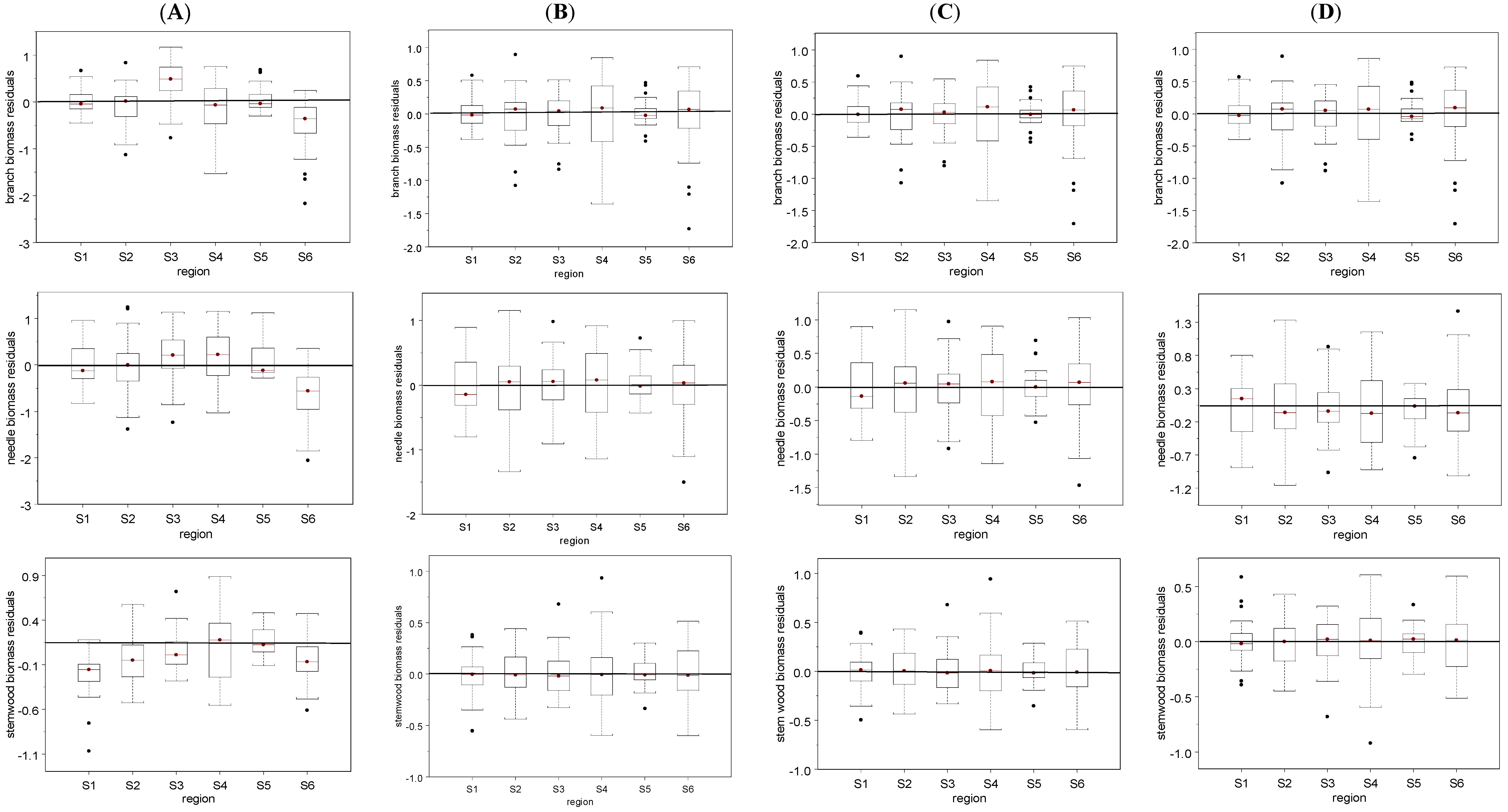

Figure 3.
The regression curves of the linear mixed model for different regions.

Table 1.
The code and basic featuresof study regions.
| Code | Site | Province | Latitude and Longitude | Climate Zone | Annual Average Temperature (°C) | Annual Precipitation (mm) | Larch Species |
|---|---|---|---|---|---|---|---|
| S1 | Changlinggang farm | Hubei province | 30.48° N, 110.02° E | Subtropics | 11.7 | 1884 | Larix kaempferi |
| S2 | Tianshui city | Gansu province | 34.09° N, 105.52° E | Warm temperate | 11 | 800 | Larix kaempferi |
| S3 | Weichang county | Hebei province | 41.43° N, 118.7° E | Temperate | 3.3 | 445 | Larix principis-rupprechtii |
| S4 | Dagujia farm | Liaoning province | 42.21° N, 124.52° E | Temperate | 6 | 806 | Larix kaempferi |
| S5 | Mengjiagang farm | Heilongjiang province | 46.32° N, 129.10° E | Cold temperate | 2.7 | 550 | Larix olgensis |
| S6 | Wuerqihan Forestry bureau | Inner Mongolia province | 49.34° N, 121.25° E | Cold temperate | 2.6 | 560 | Larix gmelinii |
Table 2.
Biomass of each larch component (kg tree−1) in six regions in China.
| Region | Sample Trees | Biomass Component | Min–Max | Mean(S.D.) | Region | Sample Trees | Biomass Component | Min–Max | Mean(S.D.) |
|---|---|---|---|---|---|---|---|---|---|
| S1 | 60 | branch | 0.81–16.97 | 10.66(0.84) | S4 | 60 | branch | 1.88–25.99 | 10.93(1.09) |
| needle | 0.46–5.7 | 3.31(0.20) | needle | 0.77–11.12 | 3.78(0.53) | ||||
| stem | 1.34–158.47 | 87.11(9.23) | stem | 0.82–181.25 | 68.96(9.78) | ||||
| bark | 0.28–16.97 | 9.49(0.84) | bark | 0.26–31.90 | 9.92(1.41) | ||||
| root | 0.63–42.57 | 20.46(2.35) | root | 2.32–50.28 | 23.59(2.25) | ||||
| total | 3.52–236.53 | 131.23(13.27) | total | 7.00–270.73 | 117.17(14.54) | ||||
| S2 | 60 | branch | 0.92–25.94 | 8.44(1.03) | S5 | 60 | branch | 0.4–26.09 | 6.28(1.13) |
| needle | 0.47–13.58 | 3.54(0.4) | needle | 0.06–7.07 | 1.64(0.26) | ||||
| stem | 2.42–306.17 | 78.41(12.24) | stem | 0.7–236.42 | 55.96(10.30) | ||||
| bark | 0.66–29.20 | 8.52(1.09) | bark | 0.35–22.96 | 6.47(1.06) | ||||
| root | 0.95–82.85 | 18.35(2.96) | root | 0.33–76.23 | 20.32(3.56) | ||||
| total | 5.44–457.74 | 117.25(17.25) | total | 2.2–362.41 | 90.68(16.07) | ||||
| S3 | 60 | branch | 0.48–27.39 | 7.01(0.96) | S6 | 60 | branch | 0.58–58.13 | 13.23(2.01) |
| needle | 0.2–8.7 | 2.28(0.31) | needle | 0.13–14.65 | 3.37(0.51) | ||||
| stem | 0.56–204.79 | 38.75(6.56) | stem | 1.53–144.4 | 35.14(5.00) | ||||
| bark | 0.22–20.19 | 5.65(0.83) | bark | 0.47–20.68 | 5.28(0.73) | ||||
| root | 0.23–76.79 | 13.20(2.33) | root | 0.41–59.34 | 11.23(1.81) | ||||
| total | 1.80–337.45 | 66.89(10.65) | total | 4.07–276.64 | 68.25(9.84) |
Table 3.
Parameter estimates of the general biomass model (Equation (2)).
| Biomass Component | Parameter | Estimate | S.D. | p-Value |
|---|---|---|---|---|
| Branch | a | −2.6813 | 0.1489 | <0.01 |
| b | 1.7831 | 0.0583 | <0.01 | |
| Needle | a | −3.2790 | 0.1748 | <0.01 |
| b | 1.5779 | 0.0685 | <0.01 | |
| Stemwood | a | −3.5205 | 0.0811 | <0.01 |
| b | 2.7278 | 0.0318 | <0.01 | |
| Stembark | a | −3.9267 | 0.0924 | <0.01 |
| b | 2.1516 | 0.0362 | <0.01 | |
| Root | a | −3.9618 | 0.0912 | <0.01 |
| b | 2.4586 | 0.0357 | <0.01 | |
| Total | a | −2.1166 | 0.0537 | <0.01 |
| b | 2.4199 | 0.0210 | <0.01 |
Table 4.
Parameter estimates of the dummy variable model(Equation (3)).
| Region | Biomass Component | Parameter | Estimate | S.D. | Region | Biomass Component | Parameter | Estimate | S.D. |
|---|---|---|---|---|---|---|---|---|---|
| S1 | Stem wood | a | −2.903 | 0.427 | S4 | Stem wood | a | −2.489 | 0.411 |
| b | 2.473 | 0.326 | b | 2.473 | 0.326 | ||||
| Stem bark | a | −3.541 | 0.449 | Stem bark | a | −3.499 | 0.405 | ||
| b | 2.049 | 0.167 | b | 2.049 | 0.167 | ||||
| Branch | a | −4.026 | 0.507 | Branch | a | −4.027 | 0.582 | ||
| b | 2.195 | 0.198 | b | 2.195 | 0.198 | ||||
| Needle | a | −4.288 | 0.656 | Needle | a | −4.214 | 0.633 | ||
| b | 1.954 | 0.207 | b | 1.954 | 0.207 | ||||
| Root | a | −3.793 | 0.482 | Root | a | −3.621 | 0.407 | ||
| b | 2.396 | 0.150 | b | 2.396 | 0.150 | ||||
| Total biomass | a | −2.084 | 0.221 | Total biomass | a | −1.780 | 0.207 | ||
| b | 2.419 | 0.105 | b | 2.419 | 0.105 | ||||
| S2 | Stem wood | a | −2.924 | 0.455 | S5 | Stem wood | a | −2.667 | 0.458 |
| b | 2.473 | 0.326 | b | 2.473 | 0.326 | ||||
| Stem bark | a | −3.637 | 0.602 | Stem bark | a | −3.651 | 0.423 | ||
| b | 2.049 | 0.167 | b | 2.049 | 0.167 | ||||
| Branch | a | −3.905 | 0.519 | Branch | a | −3.997 | 0.566 | ||
| b | 2.195 | 0.196 | b | 2.195 | 0.206 | ||||
| Needle | a | −4.332 | 0.639 | Needle | a | −4.510 | 0.701 | ||
| b | 1.954 | 0.207 | b | 1.954 | 0.207 | ||||
| Root | a | −3.698 | 0.356 | Root | a | −3.783 | 0.408 | ||
| b | 2.396 | 0.150 | b | 2.396 | 0.150 | ||||
| Total biomass | a | −2.078 | 0.233 | Total biomass | a | −1.943 | 0.208 | ||
| b | 2.419 | 0.105 | b | 2.419 | 0.105 | ||||
| S3 | Stem wood | a | −2.924 | 0.398 | S6 | Stem wood | a | −2.728 | 0.410 |
| b | 2.473 | 0.326 | b | 2.473 | 0.326 | ||||
| Stem bark | a | −3.571 | 0.308 | Stem bark | a | −3.643 | 0.305 | ||
| b | 2.049 | 0.167 | b | 2.049 | 0.167 | ||||
| Branch | a | −2.983 | 0.592 | Branch | a | −4.097 | 0.444 | ||
| b | 2.195 | 0.198 | b | 2.195 | 0.198 | ||||
| Needle | a | −3.683 | 0.621 | Needle | a | −4.793 | 0.655 | ||
| b | 1.954 | 0.207 | b | 1.954 | 0.207 | ||||
| Root | a | −3.641 | 0.396 | Root | a | −3.451 | 0.428 | ||
| b | 2.396 | 0.150 | b | 2.396 | 0.150 | ||||
| Total biomass | a | −1.864 | 0.207 | Total biomass | a | −1.931 | 0.197 | ||
| b | 2.419 | 0.105 | b | 2.419 | 0.105 |
Table 5.
Parameter estimates of the mixed effects model (Equation (4)).
| Biomass Component | Parameter | Estimate Values | S.D. | T-Value | p-Value |
|---|---|---|---|---|---|
| Stem wood | a | −3.684 | 0.284 | 12.983 | <0.01 |
| b | 2.783 | 0.102 | 27.233 | <0.01 | |
| σa | 0.068 | ||||
| σb | 0.008 | ||||
| σab | −0.024 | ||||
| ε | 0.223 | ||||
| Stem bark | a | −3.971 | 0.145 | 27.256 | <0.01 |
| b | 2.166 | 0.053 | 40.534 | <0.01 | |
| σa | 0.068 | ||||
| σb | 0.008 | ||||
| σab | −0.024 | ||||
| ε | 0.304 | ||||
| Branch | a | −2.668 | 0.314 | 8.485 | <0.01 |
| b | 1.783 | 0.141 | 12.662 | <0.01 | |
| σa | 0.491 | ||||
| σb | 0.104 | ||||
| σab | −0.207 | ||||
| ε | 0.384 | ||||
| Needle | a | −3.091 | 0.553 | 5.592 | <0.01 |
| b | 1.515 | 0.207 | 7.331 | <0.01 | |
| σa | 1.673 | ||||
| σb | 0.233 | ||||
| σab | −0.604 | ||||
| ε | 0.475 | ||||
| Root | a | −3.484 | 0.433 | 8.509 | <0.01 |
| b | 2.370 | 0.150 | 15.820 | <0.01 | |
| σa | 1.079 | ||||
| σb | 0.128 | ||||
| σab | −0.370 | ||||
| ε | 0.247 | ||||
| Total | a | −2.110 | 0.206 | 10.225 | <0.01 |
| b | 2.419 | 0.079 | 30.455 | <0.01 | |
| σa | 0.241 | ||||
| σb | 0.189 | ||||
| σab | −0.091 | ||||
| ε | 0.142 |
Table 6.
Parameter estimates of the Bayesian hierarchical model (Equation (5)).
| Region | Biomass Component | Parameter | Estimate Value | S.D. | Region | Biomass Component | Parameter | Estimate Value | S.D. |
|---|---|---|---|---|---|---|---|---|---|
| S1 | Stem wood | a | −4.284 | 0.210 | S4 | Stem wood | a | −3.843 | 0.153 |
| b | 3.061 | 0.080 | b | 2.836 | 0.061 | ||||
| Stem bark | a | −3.916 | 0.118 | Stem bark | a | −3.965 | 0.111 | ||
| b | 2.166 | 0.046 | b | 2.142 | 0.043 | ||||
| Branch | a | −2.354 | 0.322 | Branch | a | −3.277 | 0.255 | ||
| b | 1.605 | 0.123 | b | 1.835 | 0.101 | ||||
| Needle | a | −2.274 | 0.421 | Needle | a | −4.225 | 0.339 | ||
| b | 1.263 | 0.161 | b | 1.717 | 0.135 | ||||
| Root | a | −4.412 | 0.222 | Root | a | −4.030 | 0.186 | ||
| b | 2.600 | 0.084 | b | 2.551 | 0.074 | ||||
| Total biomass | a | −2.650 | 0.137 | Total biomass | a | −2.540 | 0.104 | ||
| b | 2.649 | 0.052 | b | 2.554 | 0.041 | ||||
| S2 | Stem wood | a | −3.356 | 0.152 | S5 | Stem wood | a | −3.007 | 0.195 |
| b | 2.671 | 0.063 | b | 2.597 | 0.071 | ||||
| Stem bark | a | −3.904 | 0.106 | Stem bark | a | −3.897 | 0.115 | ||
| b | 2.150 | 0.043 | b | 2.153 | 0.042 | ||||
| Branch | a | −3.387 | 0.282 | Branch | a | −1.989 | 0.343 | ||
| b | 2.287 | 0.118 | b | 1.543 | 0.125 | ||||
| Needle | a | −4.702 | 0.337 | Needle | a | −1.659 | 0.422 | ||
| b | 2.268 | 0.141 | b | 1.020 | 0.154 | ||||
| Root | a | −4.653 | 0.170 | Root | a | −3.135 | 0.219 | ||
| b | 2.705 | 0.071 | b | 2.138 | 0.080 | ||||
| Total biomass | a | −2.298 | 0.095 | Total biomass | a | −1.451 | 0.134 | ||
| b | 2.519 | 0.040 | b | 2.208 | 0.049 | ||||
| S3 | Stem wood | a | −3.114 | 0.122 | S6 | Stem wood | a | −4.394 | 0.25 |
| b | 2.525 | 0.051 | b | 2.971 | 0.091 | ||||
| Stem bark | a | −3.927 | 0.102 | Stem bark | a | −3.971 | 0.134 | ||
| b | 2.146 | 0.042 | b | 2.151 | 0.048 | ||||
| Branch | a | −2.757 | 0.192 | Branch | a | −2.374 | 0.381 | ||
| b | 1.794 | 0.081 | b | 1.673 | 0.138 | ||||
| Needle | a | −2.958 | 0.258 | Needle | a | −2.867 | 0.477 | ||
| b | 1.429 | 0.108 | b | 1.434 | 0.173 | ||||
| Root | a | −3.929 | 0.133 | Root | a | −2.041 | 0.314 | ||
| b | 2.434 | 0.056 | b | 1.829 | 0.114 | ||||
| Total biomass | a | −1.849 | 0.076 | Total biomass | a | −1.878 | 0.159 | ||
| b | 2.277 | 0.032 | b | 2.307 | 0.058 |
Table 7.
Evaluation statistics of the general model, dummy variable model, mixed effects model, and Bayesian hierarchical model for biomass modeling.
Table 7.
Evaluation statistics of the general model, dummy variable model, mixed effects model, and Bayesian hierarchical model for biomass modeling.
| Model | Biomass Component | R2 | MAB | RMSE | F-Value | p-Value |
|---|---|---|---|---|---|---|
| General model | Stem wood | 0.967 | 0.213 | 0.275 | ||
| Dummy variable model | 0.977 | 0.169 | 0.230 | 18.610 | <0.01 | |
| Mixed effect model | 0.979 | 0.165 | 0.222 | 12.733 | <0.01 | |
| Bayesian hierarchical model | 0.987 | 0.166 | 0.219 | 11.532 | <0.01 | |
| General model | Stem bark | 0.934 | 0.224 | 0.313 | ||
| Dummy variable model | 0.935 | 0.217 | 0.310 | 2.955 | <0.01 | |
| Mixed effect model | 0.938 | 0.213 | 0.305 | 1.339 | <0.01 | |
| Bayesian hierarchical model | 0.937 | 0.217 | 0.303 | 1.256 | <0.01 | |
| General model | Branch | 0.790 | 0.361 | 0.505 | ||
| Dummy variable model | 0.857 | 0.279 | 0.392 | 25.911 | <0.01 | |
| Mixed effect model | 0.880 | 0.269 | 0.382 | 17.713 | <0.01 | |
| Bayesian hierarchical model | 0.879 | 0.272 | 0.378 | 16.321 | <0.01 | |
| General model | Needle | 0.682 | 0.456 | 0.592 | ||
| Dummy variable model | 0.776 | 0.372 | 0.487 | 20.019 | <0.01 | |
| Mixed effect model | 0.799 | 0.355 | 0.471 | 13.713 | <0.01 | |
| Bayesian hierarchical model | 0.798 | 0.356 | 0.465 | 12.722 | <0.01 | |
| General model | Root | 0.950 | 0.236 | 0.309 | ||
| Dummy variable model | 0.967 | 0.186 | 0.247 | 20.237 | <0.01 | |
| Mixed effect model | 0.968 | 0.184 | 0.246 | 13.785 | <0.01 | |
| Bayesian hierarchical model | 0.968 | 0.185 | 0.242 | 12.695 | <0.01 | |
| General model | Total biomass | 0.982 | 0.140 | 0.182 | ||
| Dummy variable model | 0.988 | 0.106 | 0.141 | 23.388 | <0.01 | |
| Mixed effect model | 0.989 | 0.105 | 0.141 | 16.056 | <0.01 | |
| Bayesian hierarchical model | 0.989 | 0.105 | 0.139 | 15.472 | <0.01 |
© 2017 by the authors. Licensee MDPI, Basel, Switzerland. This article is an open access article distributed under the terms and conditions of the Creative Commons Attribution (CC BY) license (http://creativecommons.org/licenses/by/4.0/).
Share and Cite
MDPI and ACS Style
Chen, D.; Huang, X.; Zhang, S.; Sun, X. Biomass Modeling of Larch (Larix spp.) Plantations in China Based on the Mixed Model, Dummy Variable Model, and Bayesian Hierarchical Model. Forests 2017, 8, 268. https://doi.org/10.3390/f8080268
AMA Style
Chen D, Huang X, Zhang S, Sun X. Biomass Modeling of Larch (Larix spp.) Plantations in China Based on the Mixed Model, Dummy Variable Model, and Bayesian Hierarchical Model. Forests. 2017; 8(8):268. https://doi.org/10.3390/f8080268
Chicago/Turabian StyleChen, Dongsheng, Xingzhao Huang, Shougong Zhang, and Xiaomei Sun. 2017. "Biomass Modeling of Larch (Larix spp.) Plantations in China Based on the Mixed Model, Dummy Variable Model, and Bayesian Hierarchical Model" Forests 8, no. 8: 268. https://doi.org/10.3390/f8080268
Note that from the first issue of 2016, this journal uses article numbers instead of page numbers. See further details here.