Simulation-Based Cost Analysis of Industrial Supply of Chips from Logging Residues and Small-Diameter Trees †


1
Department of Forest Biomaterials and Technology, Swedish University of Agricultural Sciences, 90183 Umeå, Sweden
2
Department of Energy and Technology, Swedish University of Agricultural Sciences, 75007 Uppsala, Sweden
*
Author to whom correspondence should be addressed.
†
This paper is an extended version of the sections published in the doctoral thesis “Improving supply chains for logging residues and small-diameter trees in Sweden”.
Forests 2020, 11(1), 1; https://doi.org/10.3390/f11010001
Submission received: 8 November 2019
/
Revised: 9 December 2019
/
Accepted: 12 December 2019
/
Published: 18 December 2019
(This article belongs to the Special Issue Supply Chain Optimization for Biomass and Biofuels)
Abstract
:Research Highlights: The use of terminals can increase supply costs by 5–11% (when compared to direct supply), but terminals help secure supply during peak demand and cope with operational problems in the supply fleet in cases where direct supply chains would be unable to meet demand on time. Background and Objectives: This work analyses the supply cost of chipped logging residues and small-diameter trees, from chipping at roadside storages to delivery to the end-user. Factors considered include demand curves (based on the requirements of a theoretical combined heat and power plant or biorefinery); demand volume; and mode of supply (direct or combined via terminal). The impact of longer trucking distances from the sites, and supply integration between forest and other land (varying relocation distances) was also assessed. Materials and Methods: The operational environment and work of a theoretical chip supplier in northern Sweden were modelled and simulated in ExtendSim®. Results: The mean supply cost of chips was 9% higher on average for combined chains than for direct chains. Given a high demand, 8% of the annual demand could not be delivered on time without using a terminal. High supply integration of forest and other land reduced supply costs by 2%. Contractors’ annual workloads were evened out by direct supply to the biorefinery (which has a relatively steady demand) or supply via-terminal independently of the end-user. Keeping distinct chips from different sites (implying that trucks were not always fully loaded) instead of mixing chips from different sites until the trucks were fully loaded increased supply costs by 12%. Conclusions: Terminals increase supply costs, but can enable demand to be met on time when direct supply chains alone might fail. Integrated supply planning could reduce supply costs by increasing the utilization of residual biomass from other land.
Keywords:
bioenergy; CHP; biorefinery; wood chips; forest biomass; discrete-event; terminal; logistics1. Introduction
Forests play a central role in the growing bioeconomy and climate change mitigation, providing renewable materials, energy and ecosystem services [1,2,3]. The increasing production of new lignocellulose-based products such as textiles, plastics and green chemicals in biorefineries (BRs) [4] will further increase the demand for forest biomass [5]. Large quantities of residual biomass could potentially be harvested sustainably in Sweden [6,7,8,9,10]. Notable sources of such biomass include logging residues (LR; tops and branches) originating primarily from clear-fellings and small-diameter trees (ST) from dense thinning forests and clearings of other land (power line corridors, roadsides, overgrown marginal land etc.). The supply of residual biomass from forest land can be integrated with that from other land, as shown by [11]. However, cost-competitive use of residual biomass requires efficient supply chains (SCs). In Sweden, bulky residual biomass is often comminuted at forest roadsides with mobile machines [12] such as forwarder-mounted chippers and chipper-trucks. The choice of comminution strategy depends on factors including the placement of the windrows in the storage site; windrows may be located by the roadside, on a larger landing or inside the stand [11]. Alternatively, uncomminuted residual biomass can be transported for chipping at terminals or at the end-user, using mobile, semi-stationary or stationary machines [13,14]. However, the cost-effectiveness of this option is limited by the inefficiency of road transport of bulky assortments (stumps, LR and undelimbed ST) other than for sub-standard (defect) industrial roundwood and delimbed ST (which can be transported from roadside to the terminal/end-user by conventional roundwood trucks).
Terminals can be important parts of biomass SCs, acting as intermediate nodes between the forest and industry that enable processes such as transloading (changing transportation modes), storage and upgrading of biomass (comminution, sieving, drying, etc.) before final delivery. Terminals for round- and fuelwood are common in Sweden, Finland and Austria; they may be placed close to the resource or the end-user, and are sometimes connected to a railway or adjacent to harbours [15,16,17,18]. Delivery via terminal inevitably introduces extra costs into the SC (compared to direct delivery) because of the investment necessary to build and maintain the terminal and increased material handling [19,20]. In addition, storage of comminuted biomass results in dry matter losses (DML) [21]. However, terminals can be essential because they increase the reliability of supply during peak demand and make it easier to cope with problems in the supply fleet such as machine breakdowns or extreme events (freeze-thaw melting, forest fires or windthrow) that may impede access to forest storage sites. Terminals also provide buffering for industries with limited storage capacity. Plants near urban areas usually have small buffers that can only store a few days’ worth of material, whereas plants outside urban areas can maintain much larger reserves [22]. A common practice in the forest fuel business is for industry and suppliers to agree on a delivery plan specifying the amount of chips to be supplied every month [23]. The demand curves of energy industries (heating plants and combined heat and power plants, CHPs) are strongly seasonal (i.e., demand is high in winter and low in summer), meaning that contractors must concentrate their operations during a few months of the year if supplying forest fuels directly from the forest. Conversely, annual demand from BRs can be expected to be relatively constant because new BRs are likely to be built around existing pulpmills [24]. Roundwood contractors commonly reduce supply around July, ramp it up in August and reach full capacity again in September, as shown by [25]. This means that contractors normally take holidays before production at the mills bottoms out and then resume supplying feedstock before the plants reach full production again. Current industries also tend to reduce or empty their stored reserves during summertime [26] and perform maintenance. Terminals can help to maintain consistent year-round operation of supply fleets, serving as storage sites during periods of machine overcapacity [27]. The need for terminals is increasing as the capacity of existing industries expands, necessitating larger uptake areas and reliable high-efficiency procurement solutions [28,29,30,31].
Simulations allow operational options for increasing efficiency, making it possible to offer advice to decision-makers without performing real-world experiments [32,33]. Discrete-event simulation has been used in several wood SC analyses [34]. For example [35], found that costs can be underestimated by circa 20% if delays caused by machine interactions and random elements (e.g., breakdowns) are neglected, which can be difficult to assess using analytical methods. Differences between static approaches and discrete-event simulations were assessed by finding that cost-efficiency could increase if machine capacity in hot systems is properly balanced and the utilization rate of comminution equipment increases [36,37]. Few simulation studies have quantified the increase in supply cost due to the use of terminals in forest chip SCs [38,39,40].
Therefore, the main aim of this study was to analyse the supply cost of chipped LR and ST, from chipping at forest storage sites to delivery to the end-user. Two end-user demand curves were considered, one for a theoretical CHP, and one for a theoretical BR. In addition, two different demand scenarios (low and high, referring to different annual demand volumes), and two possible modes of supply chain operation were considered: exclusive direct supply from the sites to the end-user and supply via a feed-in terminal (a combination of direct and via-terminal deliveries). Sensitivity analyses were conducted to evaluate the impact of varying the trucking distance from the sites to the terminal/end-user, and of chip supply integration between forest and other land (i.e., increasing/decreasing relocation distances).
2. Materials and Methods
2.1. General Description of the Model and Biomass Characteristics
A simulation model was constructed using discrete-event simulation in ExtendSim 9.2® [41,42]. An operational environment was designed to represent the environment of chipping operations in northern Sweden (resembling that studied by [11]) and the work of a theoretical chip supplier over one year was modelled. The model’s goal was to provide the defined end-users (a theoretical CHP and a theoretical BR) with chips from a mixture of LR and undelimbed ST seasoned in windrows at forest and other land storage sites (henceforth referred to as sites). To mimic real-world operations, the model included stochasticity based on probability distributions for biomass characteristics, process times (for machine activities), delays, and forecasted demand. Probability distributions for biomass characteristics were derived from a survey of 34 sites (which collectively contained 76 windrows) in the vicinity of Umeå (northern Sweden) reported by [11]. The surveyed characteristics were analysed using Stat::Fit® [43], to find probability distributions fitting the fieldwork data. Biomass harvesting had been conducted by conventional operations (clear fellings and thinnings) in forest land at 65% of the sites, by harvesting other land (overgrown edges of arable land, roadsides and industrial land) at 26% of the sites, and by a mixture of forest and other land operations in the remaining 9% of sites.
The simulation generated entities, dry tonnes (t) of chips, batched them into windrows and subsequently into sites and were chipped by two machine systems, which delivered chips to the end-user’s buffer (plant yard) (Figure 1). Attributes (Table 1) were allocated to the generated entities based on the derived probability distributions. The simulation made no distinction between assortments (a mixture was assumed), types of harvest (forest or other land) or forest owners. Input data were inserted directly into the model blocks, while relevant output data were exported to a spreadsheet for further analysis (Figure 2).
2.2. Demand and Supply
The supply of chips was modelled separately for two theoretical end-users with distinct demand profiles: a CHP and a BR (Figure 3). Both end-users were assumed to be located at the same place and consume the same chipped feedstock. Further processing of the incoming chips at the plant was outside the model’s boundaries. The CHP’s demand curve was derived from data on mean production at Dåva 2 in Umeå (565 GWh per year during 2012–2016, fuelled with a mix of biomasses) provided by Umeå Energi AB. The CHP’s demand peaked in January and was zero during July and August (in real-world operation, another plant fuelled with household waste met summer demand). The BR’s demand was assumed to be zero in July and August and constant otherwise (i.e., non-seasonal). Two demand scenarios (with different volumes of demand) were defined: low, corresponding to a demand of 21,000 dry t per annum, and high (29,000 dry t per annum). In both scenarios, it was assumed that the demand would be met by sites located at a maximum road distance of 99 km (one-way) from the plants (Table 1). A monthly delivery plan for the modelled chip supplier was calculated for each demand volume and end-user, matched against the monthly shares of forecasted demand. The delivery plan was calculated on a daily basis and interpolated to smooth increments and decrements between consecutive days (Figure 3). Since real volumes of demand and supply deviate from forecasts, a deviation of ±20% relative to forecasted values was incorporated, as in [40]. An average energy content of 4.8 MWh dry t−1 (for a mixture of LR and ST) was considered, calculated on the basis of a gross heating value of 19.8 MJ dry kg−1, an average moisture content (MC) of 45.3% (wet-basis) and ash content of 1.85% (dry-basis), as found during the fieldwork in [11].
2.3. Terminal Characteristics
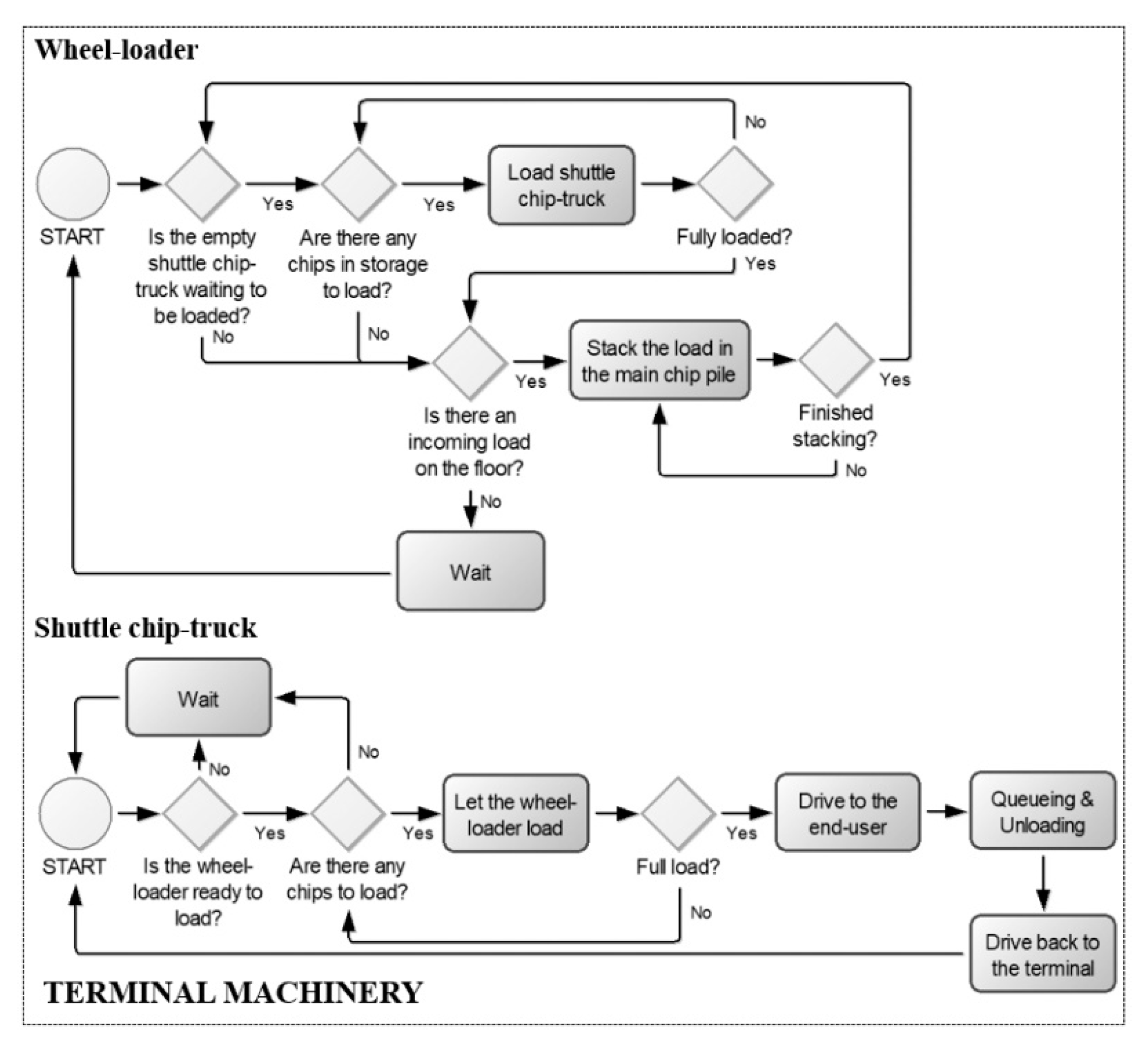
Two possible modes of SC operation were modelled in the simulation: exclusive direct supply from the sites to the end-user (“direct supply” henceforth) and supply via a feed-in terminal (a combination of direct and via-terminal deliveries, “combined supply” henceforth). The terminal was used for chip storage, primarily to increase supply reliability. A shuttle chip-truck was available, driving a 10 km (one-way) distance between the terminal and the end-user. A wheel-loader operated at the terminal, equipped with a scale to measure outbound deliveries and avoid overloading the shuttle chip-truck. Facilities and machinery were shared with other suppliers, but machinery was assumed to be available whenever needed (i.e., without waiting time) for the modelled supplier. The terminal lacked equipment such as a weighbridge and drying oven. Therefore, drivers of incoming trucks were expected to measure the chip volume in the cargo and the chips’ MC using handheld equipment. The logic of the terminal machines’ work is illustrated in Figure 4.
The terminal’s storage capacity when supplying the CHP was assumed to be identical to that when supplying the BR, corresponding to a buffer time of 1 month at the CHP (based on demand in January). Therefore, its maximum storage capacity (for the modelled supplier) was set to 3425 and 4729 dry t for the low- and high-demand scenarios, respectively. The area requirements for the chosen storage capacities were 4391 and 6063 m2, respectively, assuming a utilization of 0.78 dry t m−2 [17]. The terminal storage was empty at the beginning of the simulation, followed the first-in-first-out queuing principle, and gates were open during the machines’ working hours. In line with [44], a DML of 2% per 30 days of storage was modelled and calculated for each dry t, leaving the terminal based on its storage time at departure. Changes in MC during storage were not modelled.
The model included a buffer at each end-user’s storage yard (i.e., the delivery point at the plant). Plant buffers were equal in capacity for the CHP and BR, full at the start of the simulation, and corresponded to 4 days of mean demand in January at the CHP. The maximum storage capacity of the plant buffer (for the modelled chip supplier) was set to 548 and 757 dry t for the low- and high-demand scenarios, respectively. No restrictions in opening times were set; it was assumed that truck drivers could access the storage yards at any point during a working shift. Alarms based on storage levels at the end-user’s buffer pulled chips downstream, thereby controlling upstream SC operations in the model. In the direct supply scenarios, if storage levels exceeded 95% of total capacity, the model paused the generation of new entities. In the combined supply scenarios, if storage levels exceeded 95% of total capacity, chips were redirected to the terminal, and the generation of new entities by the model was paused; for levels between 60–95%, only direct deliveries from the sites were allowed; and when storage levels at the buffer fell below 60%, the terminal was opened for outbound deliveries, thus, combining direct and via-terminal deliveries. The same alarm levels were set for both the CHP and the BR, aiming to achieve a chip flow through the terminal of 10–30% of total supply, as in real-world operation [23,45,46].
2.4. Systems for Comminution and Transport to the Terminal or End-User
2.4.1. Description of Systems
The modelled fleet working for the chip supplier (for both direct and combined supply) consisted of two systems for comminution and transport of biomass from the sites (Figure 5), with one unit of each system. The simulated systems were identical for all scenarios save for the terminal machinery, which was exclusively used in combined SCs. The machine capacity was independent of the simulated demand volume (low or high) and end-user (CHP or BR). The model was designed such that systems could not compete; thus, all work of a particular type at any given site was conducted by the same system.
System 1 comprised a forwarder-mounted chipper (Bruks 805 CT, with a self-dumping chip-bin of 21 m3) and two self-loading chip-trucks. The chipper worked by the forest roadsides or inside the stand in cases where windrows were unreachable from the road, and tipped over the chip-bin by the roadside. Afterwards, the self-loading chip-trucks loaded and transported the chips to the terminal or end-user, depending on the current alarm levels at the plant buffer. Relocation of the forwarder-mounted chipper between sites was performed by driving on the road by itself (over short distances) or by a truck with a low-bed trailer. The break-even distance for selecting between relocation modes was set to 10 km based on practice and cost calculations described by [47].
System 2 consisted of a chipper-truck (of the same make as in System 1) used for roadside comminution and transport to the terminal or end-user (Figure 5). In practice, windrows must be within circa 9 m of the roadside to be reached by the chipper-truck [11]. It was found that about 42% of the sampled windrows were not reachable from the roadside. Therefore, this proportion of sites was prioritised to System 1, and the rest could be handled by either system. The distribution of site characteristics was randomised to maximise the similarity of the sites handled by the two systems.
2.4.2. Input Data
Table 2 and Table 3 present efficiency data for the modelled machines based on literature measurements conducted in Swedish or similar operational environments resembling those considered in the model. The input data were based on an average for LR and undelimbed ST (i.e., a mixture of biomass types was assumed). Efficiency data for the forwarder-mounted chipper were reported by [48] and corresponded to its operation in the windrow storages described by [11]. Data for the chipper-truck were obtained by [48,49,50]. Since the generated sites could contain multiple windrows, the relocation of machines between windrows was also modelled (resulting in extra terrain driving). The mean time to repair the comminution equipment was assumed to follow a triangular distribution (minimum, mode, maximum), triang (0.1, 10, 136) min, derived from the work of [51]. The wheel-loader’s mean time to repair (5 min) was assumed to follow a negative exponential distribution. The mean time between failures was adjusted in the simulation environment such that machines worked according to the utilization rates specified in Table 4. Utilization rate for the forwarder-mounted chipper was derived from the work of [51], and [52] for the rest of machines.
The mean driving speed of all trucks (empty and loaded) was assumed to vary log-normally according to Equation (1), as in [53,54], where v denotes the average speed (km h−1) and d denotes the one-way transport distance (km):
The model dynamically computed the size of every chip load in every truck, which depended on the current chip MC and was limited by the truck frame (cargo) volume, tare weight and Sweden’s legally imposed upper payload limit of 64 tons [55]. As highlighted by [54], the limiting factor for relatively dry material would be the cargo volume, but weight would be limiting for relatively wet material. A break-even MC value for the transition between these two regimes was calculated (Table 3) based on the truck’s specifications and a chip loose volume of 6.2 m3 dry t−1 [56]. Trucks were only allowed to drive to the terminal or end-user if they were fully loaded, thus, they had to relocate between sites until reaching a full load. Truck efficiency data were obtained from [57]. Since queues of trucks may form at the delivery point of the terminal or end-user during real operation [58,59], a queuing time was added based on the triangular distribution triang (0, 5, 15) min. Transportation from the terminal to the end-user was performed by a shuttle chip-truck. The productive time consumption of the wheel-loader was set to 1.1 min per bucket (stacking) and 1.7 min per bucket (loading) based on the work of [52]. The volume of its bucket (10 m3) limited the chip load size to 1.6 dry t.
2.4.3. Working Shifts
Machines were scheduled to work 200 days annually (Monday to Friday), using the same shift configuration for both end-users. Therefore, in the simulation environment, the machines were set off-shift from the middle of June to the end of August (i.e., it was assumed that the annual holidays of personnel would be concentrated during this period). The length of single shifts was set to 8 h, with a 0.5 h lunch break after 4 h. From September to the end of February, the forwarder-mounted chipper, self-loading chip-trucks and chipper-truck were scheduled to perform double shifts per day (0.5 h break between shifts to change driver). From March until the middle of June, these machines performed single shifts per day, halving the chip flow from forest roadsides. This was done to simulate an extreme weather event, as observed during fieldwork in [11]. It was assumed that the forest roads would sometimes be untrafficable during March-May due to freeze-thaw and snow melting (allowing the machines to operate for only one shift per day on average), and because of the need to avoid soil damage. Single shift operation was assumed from May to June because of the decline in demand (Figure 3) and to avoid accumulating large stocks of material at the terminal during summer. Based on these shift configurations, the summed scheduled working time for the forwarder-mounted chipper, self-loading chip-trucks, and chipper-truck amounted to 2648 scheduled machine hours (SMh) each. SMh comprised machine working time including delays due to operator or mechanical breakdowns and maintenance, and machine relocation. Eventual return to garage during off-shift time was not modelled; it was assumed that changes of driver between shifts could occur elsewhere than the garage. The wheel-loader and shuttle chip-truck were scheduled to work double shifts from September to the end of April, and single shifts from May to the middle of June, amounting to 2992 SMh each.
2.5. Cost Calculation
The hourly cost of machines and the terminal operational cost (Table 4 and Table 5) were computed using the “FLIS” machine-cost calculator [52], which is based on the work of [60,61]. The terminal operational cost (i.e., the cost of handling biomass passing through the terminal) included the costs of one managerial employee and the establishment costs presented by [20]. All calculations assumed a 5.5% interest rate and were performed from the contractor’s point of view, including wages but excluding margin for profit or risk. Hourly costs were calculated on the basis of year-round double shifts (3200 SMh) even though the simulated machines were only available to work for the modelled chip supplier for either 2648 or 2992 SMh. This assumption meant that contractors were expected to work for other suppliers during off-shift time in the model (and during idle time due to lack of material) until reaching 3200 SMh. The hourly cost of a truck with a low-bed trailer to relocate the forwarder-mounted chipper was set to 106 € SMh−1. These relocations, in addition to driving time to the next site, included 70 min per relocation for the truck (driving to the current site, loading and unloading the chipper) and 45 min for the forwarder-mounted chipper (waiting for the truck, loading and unloading).
The total supply cost (€) comprised the modelled operations in the SC (comminution and transport), relocations and terminal activities (wheel-loader operation, shuttle chip-truck operation and terminal operational cost). Total supply cost included the production cost of biomass lost during terminal storage in combined SCs. Mean supply cost (€ dry t−1) was calculated as the total supply cost divided by the actual delivered biomass to the end-user. Costs due to machine idling, stumpage, tied up capital at roadsides/terminal storages, snow shovelling (to access the sites and clean the terminal) and upstream forest operations (e.g., harvesting and forwarding) were excluded. An exchange rate of 1 € (euro) = 9.6 SEK (Swedish krona) was used.
2.6. Experimental Design
Simulations were performed for eight defined scenarios (Table 6). Inputs and system configurations were kept constant between runs. Five replicate simulations were performed for each scenario. Results were compared by one-way ANOVA with Tukey’s post-hoc test, using a significance threshold of p < 0.05.
2.7. Sensitivity Analysis
Sensitivity analysis was performed in scenarios 3, 4, 7 and 8, i.e., those with high end-user demand volumes (Table 6). These analyses examined the cost impact of increasing the site-to-terminal or site-to-end-user trucking distances by 25 and 50%, while keeping the terminal-to-end-user trucking distance constant. The cost impact of supply integration of chips from forest and other land was also investigated based on the assumption that an integrated biomass supply from multiple sources should increase biomass concentrations and reduce relocation distances between storage sites. To this end, analyses were performed assuming a “high” level of integration with 50% shorter relocation distances, and a “low” level involving 50% longer relocation distances. Each analysis was run in five replicates. The results of the sensitivity analysis were compared to the ground settings for scenarios 3, 4, 7 and 8 by one-way analysis of variance (ANOVA) with Tukey’s post-hoc test, using a significance threshold of p < 0.05.
2.8. Verification and Validation
The model built in ExtendSim® was verified using subjective methods, namely visualization (assisted by the software’s graphical interface) and walkthroughs [62]. Model validation was performed using both subjective and objective approaches, including a discussion with experts familiar with the modelled systems (including forest practitioners), checking that the model’s behaviour reproduced that of real systems, and checking that some of the model’s key preliminary outputs (relating to factors such as machine efficiency, work time elements’ distribution and costs) were consistent with previous studies. All these tests indicated the model to be reasonable.
3. Results
3.1. Main Results
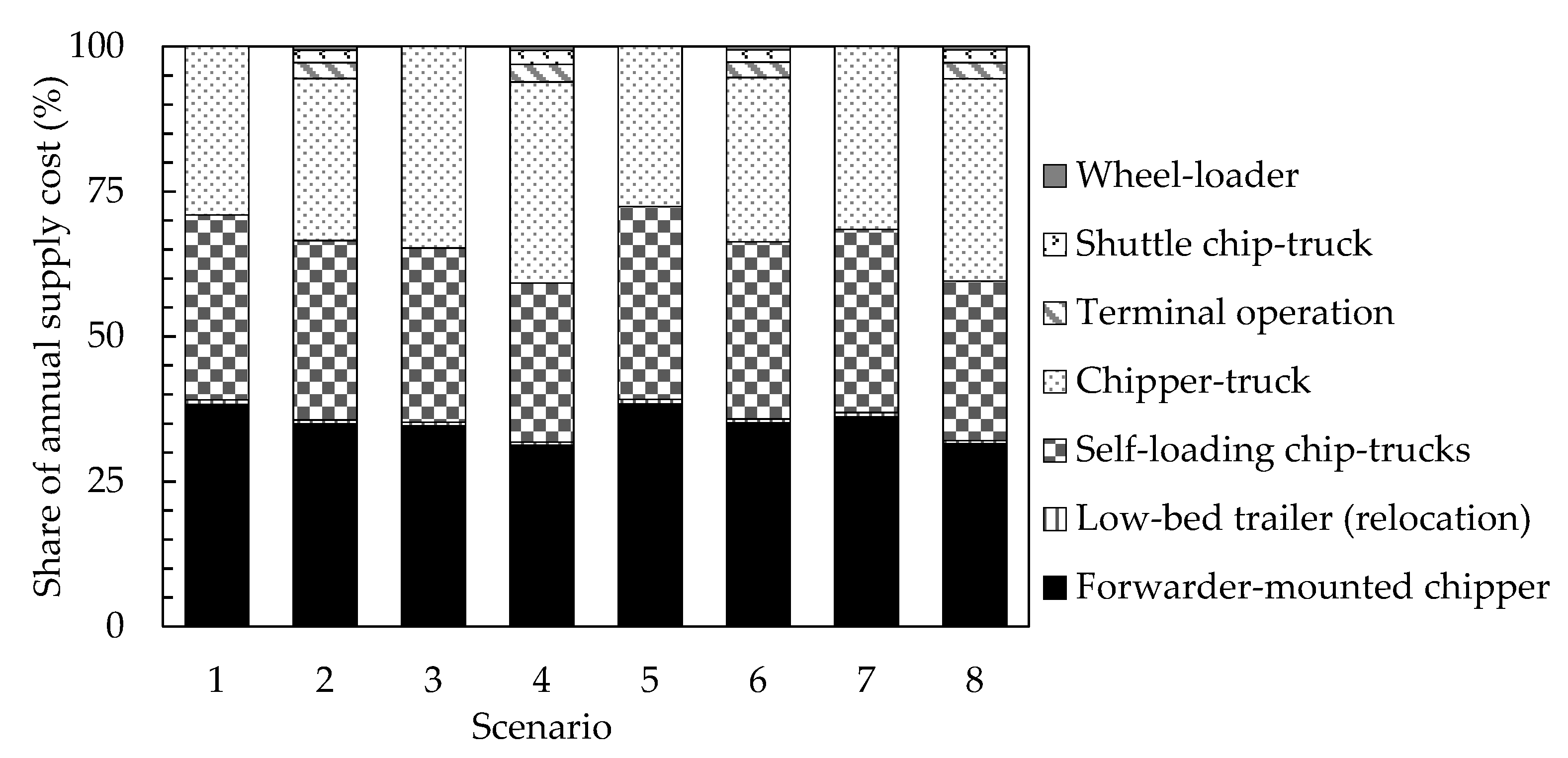
The simulations revealed that the mean supply cost of chips (Table 7) was 9% higher on average (47.0 versus 43.2 € dry t−1, range: 5–11%) in the combined SC scenarios than the direct SC scenarios. The cost of direct and combined supply to the CHP averaged 42.7 € dry t−1 and 47.0 € dry t−1 across scenarios, respectively, while those of direct and combined supply to the BR averaged 43.8 € dry t−1 and 47.0 € dry t−1, respectively. No significant differences in mean supply costs or annual supply costs of chips (evaluated by comparing scenario 2 against 6 and 4 against 8) were found between end-users in the combined supply scenarios. Nevertheless, direct supply to the BR yielded a 3% higher mean cost than direct supply to the CHP. System 1 (comprising a forwarder-mounted chipper and two self-loading chip-trucks) accounted for 59–72% of the annual supply costs, including relocations (Figure 6), while System 2 (chipper-truck) was responsible for 28–35%. The higher priority given to System 1 led to a comparatively high use of the forwarder-mounted chipper (Figure 7), explaining its larger share of the total supply cost. System 1 also had an 8% higher operational cost than System 2 (44.2 versus 40.8 € dry t−1) (Table 8). Terminal activities (wheel-loader operation, shuttle chip-truck operation and terminal operational cost) accounted for 5–6% of the annual supply cost in the combined SCs.
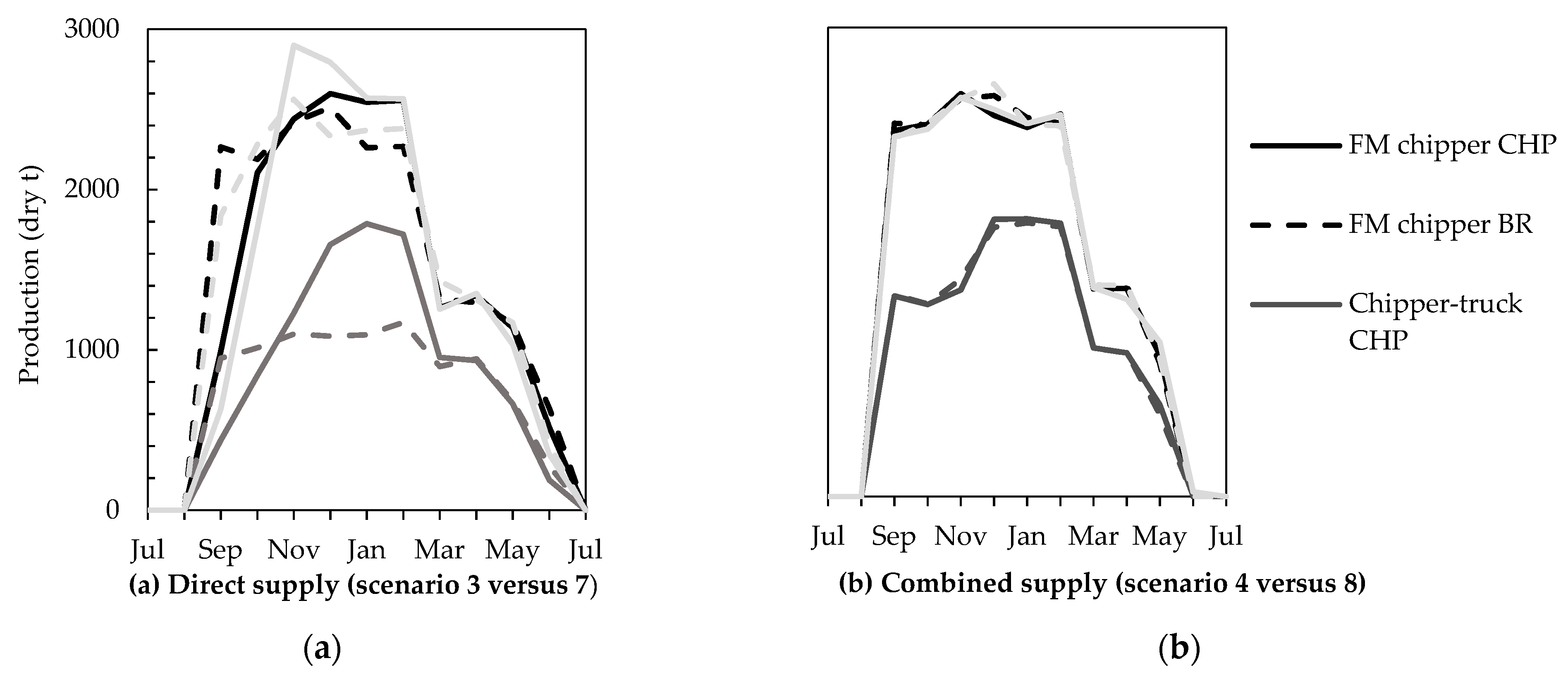
The actual use (spent SMh divided by available SMh in the simulation) of machines was similar between end-users, but combined scenarios enabled higher use than direct supply scenarios, especially for the chipper-truck (whose use was 3–19% higher in combined scenarios) (Figure 7). Comminution machinery was highly used in the high-demand scenarios: the use rates for the forwarder-mounted chipper and chipper-truck were 100% and 78–97%, respectively. The actual use rates of the self-loading chip-trucks were between 41–53% per truck, while those for the shuttle chip-truck and wheel-loader were 5–10% and 3–5%, respectively. The distribution of workload (represented by monthly production) over the year when supplying the BR directly (Figure 8) was more even than when directly supplying the CHP, which has a seasonal demand (Figure 3). Additionally, regardless of the end-user, combined supply via terminal evened out the contractors’ annual workload. The forwarder-mounted chipper and chipper-truck spent 53% and 37% of their productive work time on chipping, respectively (Figure 9).
3.2. Material Flows
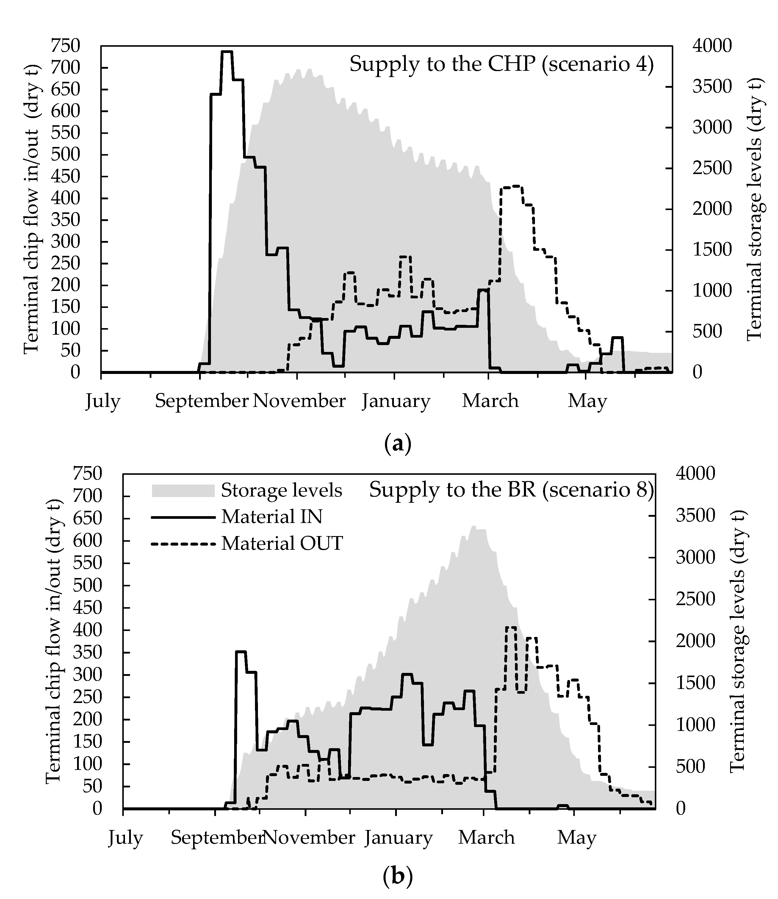
In the low-demand scenarios (1, 2, 5 and 6), the modelled chip supplier provided all biomass on time (Table 9). In the high-demand scenarios, supply was only delivered on time in the combined supply scenarios (4 and 8). In direct supply scenarios (3 and 7), a volume representing circa 8% of the annual demand was not provided on time. In scenario 3, the CHP’s demand was not met on time for several days in January and February, and also for several days from March until the beginning of May. In scenario 7, the BR’s demand was not met on time for several days from the middle of March until the middle of May. For combined SC scenarios, at the high-demand volume, the amount of biomass passing through the terminal ranged between 15 and 17% of total supply (4486–4927 dry t, in scenario 4 and 8, respectively). When supplying the CHP (Figure 10), the storage of material at the terminal increased from September and peaked in November. Outbound deliveries began at the end of October and increased in December and January. The majority of outbound deliveries occurred between the end of February and the beginning of May, greatly reducing the storage level at the terminal. Conversely, when supplying the BR, terminal storage accumulated more uniformly, peaking at the beginning of March. The majority of outbound deliveries occurred from March onwards.
Mean storage time at the terminal was 4–22% greater when supplying the CHP than the BR (28 versus 27 weeks and 15 versus 12 weeks, in the low and high-demand scenarios, respectively) (Table 10). The longer storage times, together with the higher mean storage levels, resulted in 12–43% greater DML when supplying the CHP than the BR (547 versus 488 dry t and 400 versus 279 dry t, in the low- and high-demand scenarios, respectively). DML when supplying the CHP corresponded to 2.5–1.4% of annual supply and 2.3–0.9% when supplying the BR, in the low- and high-demand scenarios, respectively.
3.3. Sensitivity Analysis
Sensitivity analyses (Table 11) revealed that increasing trucking distances from sites to the terminal/end-user by 25% (from circa 40 to 50 km) increased supply costs by 5% on average, while increasing trucking distances by 50% (from circa 40 to 60 km) increased them by 11%. Increasing trucking distances by 25 and 50% increased the chipper-truck’s operational cost by 8 and 15%, respectively, and increased that of the self-loading chip trucks by 10 and 19%, respectively. Reducing the integration of chip supply from forests and other land (increasing relocation distances from circa 13 to 20 km) increased supply costs by circa 2% based on the average for both end-users. Conversely, increasing integration (by reducing relocation distances from circa 13 to 7 km) when supplying the CHP reduced mean supply costs by circa 2%. A similar decrease was observed when supplying the BR directly (scenario 7), but the decrease was not significant (p = 0.065) when compared to combined supply (scenario 8). The mean operational cost of the forwarder-mounted chipper (which includes the cost of relocations) increased by 4% upon reducing integration (Table 12) and decreased by 4% upon increasing integration. The effect of supply integration was not significant for the chipper-truck (p = 0.550 and p = 0.847 for low and high integration, respectively).
4. Discussion
This study demonstrated the importance of terminals for increasing the reliability of supply. Relying only on direct deliveries was feasible in the low-demand scenarios, in which case using a terminal could be seen as an unnecessary cost. Conversely, at higher volumes of demand, the agreed volumes could only be delivered on time when using the terminal. On average for scenarios 4 and 8, the terminal increased mean supply cost by 7% (Table 7). However, if the terminal was not used (scenario 3 and 7), 8% of the annual demand could not be delivered on time (Table 9). The cost of not meeting demand on time (which could bring the plant to a standstill) can be difficult to quantify in real-world operation of industries (such as a CHP or a BR plant), thus, it may be convenient to use a terminal to reduce risks despite the quantified increase in the cost of supply. The simulation assumed a single theoretical supplier. In reality, the total demand can be met by only one (often, small heating plants but also large CHP plans) or several dealers. Deviations from the delivery plans may be compensated by purchase from other suppliers [63]. Therefore, if one supplier failed to provide an agreed volume on time, the end-user would attempt to buy supplementary material from another dealer. Alternatively, the current dealer could increase its machine capacity by temporarily hiring other contractors. However, other industries may face similar problems at the same time, leading to competition for raw material and labour in the area (probably leading to shortages and cost increases). The simulated demand volumes (low: 21,000 dry t, high: 29,000 dry t) represented circa 40 and 55%, respectively, of the mean supply of primary forest fuels for heat and power in Umeå (256 GWh per year during 2012–2016) [64].
The supply costs for combined SCs were 5–11% higher than for direct SCs (Table 7), in keeping with the results of [39], 7–9%, and [40], 2–12%. However, in absolute terms, the mean supply cost in our study was 19–27% higher than that reported by [40], due to differences in machine systems and model settings. In general, the choice of comminution strategy is determined by aspects of the operational environment [65] such as the placement of the windrows, transport distances to the end-user and legislation. According to [37], there is no perfect system; each one has its own advantages and drawbacks. Our average cost of direct supply (43.2 € dry t−1) of LR and ST is on the lower end of the range of stump supply costs reported by [54]. However, direct comparisons with other simulation studies can be difficult and misleading because specific results are only valid for a given set of input data and relationships between model components (which are often unique to the case study), and should not be extrapolated to other regions or countries.
Material flowed relatively steadily through the terminal when supplying the BR, because unlike the CHP (Figure 3), its demand profile was not seasonal (Figure 10). The variation in storage levels when supplying the CHP was similar to that reported by [66]. The amount of material flowing through the terminal ranged from 15 to 17% of the total supply, in keeping with the findings of [40]; this may be partly because both studies used similar alarm levels. The analysis revealed (Figure 8) that direct supply of feedstock to the BR and combined supply via-terminal to the CHP or the BR evened out the contractors’ annual workload, enabling more steady operation. DML during terminal storage were 12–43% higher when supplying the CHP than when supplying the BR (Table 10). When managing terminals, DML should be minimised by using optimal storage methods, as shown by [67], and finding a balance between maintaining low storage levels and being able to rapidly fulfil demand when required [68].
Found that site size, trucking distance and machine productivity were the factors with the largest impact on the supply cost of stumps. Sensitivity analyses (Table 11 and Table 12) indicated that mean supply cost increased by 5–11% upon increasing trucking distances by 25–50%. The simulation used real trucking distances (Table 1) from a case study, and assumed that sufficient biomass would be available within a road distance of 99 km from the plants (37 km on average). Nevertheless, the transportation distances considered in the simulation were shorter than the average for primary forest fuels in northern Sweden (66 km) [69]. Therefore, the real biomass availability in the study area should be accounted to better estimate transportation costs. Neither transportation nor relocation distances were optimised in the simulation, which could have reduced total supply costs. However, [11] observed that the real-world operation of the chipper differed from the planning: the chipper often deviated from planned routes to find alternative sites because some forest roads became untrafficable due to freeze-thaw and snow melting during March–April.
The simulation used MC of supplied chips (Table 1) from a single case study [11]. These MC measurements were originally made during the period March–April, but they were used throughout the year in the simulation. For instance, 95% of MC values were found to be between 44–48%, which can be considered a narrow range of variation when compared to other studies [40,70]. Therefore, seasonal variations in MC of supplied chips should be expected if using larger datasets (lower MC for chips delivered in summer, higher MC in winter), as shown by [71]. This would affect the simulation results, since a higher or lower MC would increase or decrease, respectively, the required amount of chips to fulfil a given demand of energy, and consequently, supply costs.
The analysis showed that mean supply costs felled by 2% upon increasing the integration of chip supply from forests and other land (by reducing relocation distances by 50%). This enabled the forwarder-mounted chipper to perform more relocations by itself. Conversely, lower integration necessitated more frequent relocation of the forwarder-mounted chipper using a truck with a low-bed trailer. Some integration of supply was assumed in the modelled operational environment because the relocation distances used in the simulations were derived from sites in forest and other land. However, the concept of supply integration should not be limited to comminution and transport; it should also encompass upstream operations such as harvesting, forwarding, and managerial work (which generates overhead costs). Therefore, the effects of integration would be greater if flexible harvesting systems were used for diverse cutting operations, which would also reduce relocation distances for harvesting machines [72]. Integration can be relevant to private forest owners’ associations because contractors work in relatively small sites and must relocate several times per year.
The use rates of the studied machines were below 100% in most scenarios (Figure 7), indicating high levels of idle time. Idle time was not accounted for in the cost calculations; hourly costs were calculated based on a working time of 3200 SMh, on the assumption that contractors would find additional work outside the model until this figure was reached. Hourly costs for machinery can be difficult to estimate, especially when performing isolated analysis as in this work. A machine’s expected annual working time strongly affects its calculated hourly costs, thus, the results presented here must be treated as only an approximation of reality. In real-world operation, transport contractors can be flexible and rapidly directed towards other landings, while chipping contractors may be confined within a smaller region due to their comparatively high relocation costs.
The logic of the work of the self-loading chip trucks (Figure 5) assumed that, after unloading at the terminal/end-user, the truck would drive back to the site if there were any chips left to load (a fact verified when unloading was finished). However, in real-world operation, truck drivers could inform each other if they could load all remaining chips at the roadside (telling the other truck to drive directly to the next site), or if there is a need to drive back to the same site. Consequently, total trucking distances may be overestimated in the simulation, resulting in higher transportation and total supply costs.
The simulation assumed that the chipper-truck and self-loading chip-trucks would relocate between sites until they were fully loaded. However, when forest owners’ associations supply chips, deliveries must be kept distinct to compensate each landowner based on the amount of energy they deliver. This requires scaling the load or measuring bulk chip volume and sampling for MC determination [73]. Consequently, trucks arriving at the terminal or end-user may not always be fully loaded. Therefore, simulations were performed to investigate the effect of keeping chips from different sites separate, allowing partially loaded trucks to drive to the end-user. This increased supply costs by 12% on average (48.2–51.5 € dry t−1 for direct and combined SCs, respectively). The integration of scales in the trucks [74] and the use of handheld equipment for MC determination [75] may allow material from different landowners to be mixed, making it easier to achieve full loads, and thus, increasing cost-efficiency. Using larger trailers with electronic steering systems can also increase SC competitiveness [76].
The methodology in our study (discrete-event simulation) has already been applied in many studies in the area of biomass SCs, as shown by [34]. However, this work contributes to expand the knowledge in the research area because of the use of detailed empirical data from a case study (low abstraction level). Combined with other studies (in turn, using data from other geographical locations), the research community can gain a greater understanding of real-world systems and identify general patterns. In addition to the supply of chips to a CHP plant (which has been extensively analysed in last decades), the current study included a BR as an alternative end-user of the biomass. If the transition towards a bioeconomy continues, the demand for forest biomass from new biorefining industries is expected to increase. Finally, this study evaluated the impact on cost of chip supply integration between forest and other lands. To our knowledge, this has not been reported before from a Swedish perspective and results indicated this should be addressed further in future research efforts.
5. Conclusions
This study showed that a terminal can help secure supply during peak demand and cope with operational problems in the supply fleet in cases where direct SCs would be unable to meet demand on time. However, more comprehensive studies are needed to assess the effect of increasing supply integration between forest and other land. The model presented here could be tailored to different cases by changing the input values and modelling alternative systems or end-users, depending on the simulation’s purpose. It could also be useful for SC engineering in industry or academia, and as a decision-support tool. The growth of the bioeconomy may spur an increase in the use of terminals as new industries flourish and existing industries increase in capacity, necessitating the construction of safe and efficient SCs.
Author Contributions
Conceptualization, D.B., R.F.-L. and A.E.; methodology, R.F.-L., A.E. and D.B.; software, R.F.-L. and A.E.; validation, R.F.-L., A.E. and D.B.; formal analysis, R.F.-L.; investigation, R.F.-L.; resources, R.F.-L.; data curation, R.F.-L.; writing—original draft preparation, R.F.-L.; writing—review and editing, R.F.-L., A.E. and D.B.; visualization, R.F.-L.; supervision, D.B. and A.E.; project administration, D.B.; funding acquisition, D.B. All authors have read and agreed to the published version of the manuscript.
Funding
This research was funded by the BOTNIA-ATLANTICA PROGRAMME (part of the European Regional Development Fund), and it was conducted within the BioHub project (http://biofuelregion.se/projekt/biohub/).
Acknowledgments
The authors gratefully acknowledged Kaj Johansson Åkeri AB, Norrlandsjord and Miljö AB, Swecon Anläggningsmaskiner AB and Mellanskog for fruitful discussions regarding the work of machine contractors and terminals; Umeå Energi AB for supplying data; and the organisations that provided financial support.
Conflicts of Interest
The authors declare no conflict of interest.
References
- Scarlat, N.; Dallemand, J.-F.; Monforti-Ferrario, F.; Nita, V. The role of biomass and bioenergy in a future bioeconomy: Policies and facts. Environ. Dev. 2015, 15, 3–34. [Google Scholar] [CrossRef]
- Berndes, G.; Abt, B.; Asikainen, A.; Cowie, A.; Dale, V.; Gustaf, E.; Lindner, M.; Marelli, L.; Paré, D.; Pingoud, K.; et al. Forest Biomass, Carbon Neutrality and Climate Change Mitigation; From Science to Policy 3; European Forest Institute (EFI): Joensuu, Finland, 2016; ISBN 978-952-5980-27-1; ISBN 978-952-5980-28-8. [Google Scholar]
- Winkel, G. Towards a Sustainable European Forest-Based Bioeconomy—Assessment and the Way Forward; What Science Can Tell Us 8; European Forest Institute (EFI): Bonn, Germany, 2017; p. 162. ISBN 978-952-5980-42-4. [Google Scholar]
- SP Processum. The Future Needs Green Alternatives– We Mean to Create Them; The Biorefinery of the Future; Processum Biorefinery Initiative AB: Örnsköldsvik, Sweden, 2016. [Google Scholar]
- Mantau, U.; Saal, U.; Prins, K.; Steierer, F.; Lindner, M.; Verkerk, H.; Eggers, J.; Leek, N.; Oldenburger, J.; Asikainen, A.; et al. EUwood – Real Potential for Changes in Growth and Use of EU Forests; Final Report; Centre of Wood Science, University of Hamburg: Hamburg, Germany, 2010. [Google Scholar]
- Fernandez-Lacruz, R.; Di Fulvio, F.; Bergström, D. Productivity and profitability of harvesting power line corridors for bioenergy. Silva. Fenn. 2013, 47. [Google Scholar] [CrossRef] [Green Version]
- Fernandez-Lacruz, R.; Bergström, D. Assessment of high-frequency technologies for determining the moisture content of comminuted solid wood fuels. Wood Mater. Sci. Eng. 2015, 11, 13–24. [Google Scholar] [CrossRef]
- Routa, J.; Asikainen, A.; Bjorheden, R.; Laitila, J.; Röser, D. Forest energy procurement: State of the art in Finland and Sweden. Wires Energy Environ. 2013, 2, 602–613. [Google Scholar] [CrossRef]
- Andersson, R.; Emanuelsson, U.; Ebenhard, T.; Eriksson, L.; Hansson, P.-A.; Hultåker, O.; Lind, T.; Nilsson, D.; Ståhl, G.; Forsberg, M.; et al. Sly – en Outnyttjad Energiresurs; Swedish Biodiversity Centre at Swedish University of Agricultural Sciences and Uppsala University: Uppsala, Sweden, 2016; ISBN 978-91-88083-10-4. [Google Scholar]
- Fernandez Lacruz, R. Improving Supply Chains for Logging Residues and Small-Diameter Trees in Sweden. Ph.D. Thesis, Department of Forest Biomaterials and Technology, Swedish University of Agricultural Sciences, Umeå, Sweden, 2019. Doctoral thesis no. 2019:44. Available online: https://pub.epsilon.slu.se/16161/ (accessed on 9 January 2019).
- Fernandez-Lacruz, R.; Bergström, D. Windrowing and fuel-chip quality of residual forest biomasses in northern Sweden. Int. J. Forest Eng. 2017, 28, 186–197. [Google Scholar] [CrossRef]
- Eliasson, L.; von Hofsten, H. Prestation och Bränsleförbrukning för en Stor Mobil Flishugg–Albach 2000 Diamant; Skogforsk: Uppsala, Sweden, 2017. [Google Scholar]
- Kuhmaier, M.; Erber, G. Research Trends in European Forest Fuel Supply Chains: A Review of the Last Ten Years (2007–2016) - Part Two: Comminution, Transport & Logistics. Croat. J. Eng. 2018, 39, 139–152. [Google Scholar]
- Wolfsmayr, U.J.; Rauch, P. The primary forest fuel supply chain: A literature review. Biomass Bioenergy 2014, 60, 203–221. [Google Scholar] [CrossRef]
- Gunnarsson, H. Supply Chain Optimization in the Forest Industry. Department of Mathematics; Linköpings universitet: Linköping, Sweden, 2007. [Google Scholar]
- Kanzian, C.; Holzleitner, F.; Stampfer, K.; Ashton, S. Regional Energy Wood Logistics—Optimizing Local Fuel Supply. Silva. Fenn. 2009, 43, 113–128. [Google Scholar] [CrossRef] [Green Version]
- Kons, K.; Bergström, D.; Eriksson, U.; Athanassiadis, D.; Nordfjell, T. Characteristics of Swedish forest biomass terminals for energy. Int. J. Forest Eng. 2014, 25, 238–246. [Google Scholar] [CrossRef]
- Kons, K. Management of Forest Biomass Terminals; Swedish University of Agricultural Sciencies, Forest Biomaterials and Technology: Umeå, Sweden, 2019. [Google Scholar]
- Eriksson, L.O.; Björheden, R. Optimal storing, transport and processing for a forest-fuel supplier. Eur. J. Oper. Res. 1989, 43, 26–33. [Google Scholar] [CrossRef]
- Virkkunen, M.; Kari, M.; Hankalin, V.; Nummelin, J. Solid Biomass Fuel Terminal Concepts and a Cost Analysis of a Satellite Terminal Concept; VTT Technical Research Centre of Finland: Espoo, Finland, 2015. [Google Scholar]
- Jirjis, R. Storage and drying of wood fuel. Biomass Bioenergy 1995, 9, 181–190. [Google Scholar] [CrossRef]
- Olsson, O.; Eriksson, A.; Sjöström, J.; Anerud, E. Keep that fire burning: Fuel supply risk management strategies of Swedish district heating plants and implications for energy security. Biomass Bioenergy 2016, 90, 70–77. [Google Scholar] [CrossRef]
- Johansson, S. Flödesstyrning av Biobränsle Till Kraftvärmeverk– En Fallstudie av Ryaverket; Department of Forest Products, Swedish University of Agricultural Sciences: Uppsala, Sweden, 2013. [Google Scholar]
- Bergström, D.; Matisons, M. Forest Refine, 2012–2014: Efficient Forest Biomass Supply Chain Management for Biorefineries—Synthesis Report; Department of Forest Biomaterials and Technology, Swedish University of Agricultural Sciences: Umeå, Sweden, 2014. [Google Scholar]
- Erlandsson, E. The Triad Perspective on Business Models for Wood Harvesting Tailoring for Service Satisfaction within Forest Owners Associations; Department of Forest Biomaterials and Technology, Swedish University of Agricultural Sciences: Umeå, Sweden, 2016. [Google Scholar]
- Swedish Forest Agency. Lager av Barrsågtimmer, Massaved och Massaflis; Swedish Forest Agency: Jonkoping, Sweden, 2018.
- Raitila, J.; Korpinen, O.-J. The Concept of Terminal in the Supply Chain; Sikanen, L., Korpinen, O.-J., Tornberg, J., Saarentaus, T., Leppänen, K., Jahkonen, M., Eds.; Natural Resources Institute Finland: Helsinki, Finland, 2016. [Google Scholar]
- Tahvanainen, T.; Anttila, P. Supply chain cost analysis of long-distance transportation of energy wood in Finland. Biomass Bioenergy 2011, 35, 3360–3375. [Google Scholar] [CrossRef]
- Ranta, T.; Korpinen, O.-J.; Jäppinen, E.; Karttunen, K. Forest Biomass Availability Analysis and Large-Scale Supply Options. Open J. Forest 2012, 2, 33–40. [Google Scholar] [CrossRef] [Green Version]
- Palander, T.S.; Voutilainen, J.J. Modelling fuel terminals for supplying a combined heat and power (CHP) plant with forest biomass in Finland. Biosyst. Eng. 2013, 114, 135–145. [Google Scholar] [CrossRef]
- Virkkunen, M.; Raitila, J.; Korpinen, O.-J. Cost analysis of a satellite terminal for forest fuel supply in Finland. Scand. J. Forest Res. 2016, 31, 175–182. [Google Scholar] [CrossRef]
- Banks, J.; Carson, J.; Nelson, B.; Nicol, D. Discrete-Event System Simulation, 5th ed.; International version; Pearson Education: Upper Saddle River, NJ, USA, 2010. [Google Scholar]
- Aalto, M. Agent-Based Modeling as Part of Biomass Supply System Research; Lappeenranta-Lahti University of Technology: Lappeenranta, Finland, 2019. [Google Scholar]
- Kogler, C.; Rauch, P. Discrete event simulation of multimodal and unimodal transportation in the wood supply chain: A literature review. Silva. Fenn. 2018, 52. [Google Scholar] [CrossRef]
- Asikainen, A. Chipping terminal logistics. Scand. J. Forest Res. 1998, 13, 386–392. [Google Scholar] [CrossRef]
- She, J.; Chung, W.; Kim, D. Discrete-Event Simulation of Ground-Based Timber Harvesting Operations. Forests 2018, 9, 683. [Google Scholar] [CrossRef] [Green Version]
- Eriksson, A. Improving the Efficiency of Forest Fuel Supply Chains; Department of Energy and Technology, Swedish University of Agricultural Sciences: Uppsala, Sweden, 2016. [Google Scholar]
- Karttunen, K.; Lättilä, L.; Korpinen, O.-J.; Ranta, T. Cost-efficiency of intermodal container supply chain for forest chips. Silva. Fenn. 2013, 47. [Google Scholar] [CrossRef] [Green Version]
- Belbo, H.; Talbot, B. Systems Analysis of Ten Supply Chains for Whole Tree Chips. Forests 2014, 5, 2084–2105. [Google Scholar] [CrossRef] [Green Version]
- Väätäinen, K.; Prinz, R.; Malinen, J.; Laitila, J.; Sikanen, L. Alternative operation models for using a feed-in terminal as a part of the forest chip supply system for a CHP plant. Gcb Bioenergy 2017, 9, 1657–1673. [Google Scholar] [CrossRef] [Green Version]
- Fernandez-Lacruz, R. Supply Chain Simulation. Available online: https://youtu.be/PSmoPRMh3tY (accessed on 5 April 2019).
- Rivera, J. Modeling with Extend; IEEE Computer Society Press: Washington, DC, USA, 1998; pp. 257–262. [Google Scholar]
- Geer Mountain Software. Stat::Fit® Version 3. Distribution Fitting Software. Available online: https://www.geerms.com/Fitting-Distributions.html (accessed on 5 December 2019).
- Nilsson, D.; Thörnqvist, T. Lagring av Flisad Grot Vid värmeverk: En Jämförande Studie Mellan Vinter och Sommar Förhållanden; Faculty of Technology, Linnaeus University: Växjö, Sweden, 2013. [Google Scholar]
- Hansson, E. Metoder För att Minska Kapitalbindningen i Stora Enso Bioenergis Terminallager; Department of Forest Products, Swedish University of Agricultural Sciences: Uppsala, Sweden, 2010. [Google Scholar]
- Asmoarp, V. Terminalstrategier För Skogsflis på Södra Skogsenergi; Department of Forest Resource Management, Swedish University of Agricultural Sciences: Umeå, Sweden, 2013. [Google Scholar]
- Jönsson, P. Hjula eller traila? Kalkylverktyg [Drive or use trailer? Calculation tool]. Available online: https://www.skogforsk.se/kunskap/kunskapsbanken/2012/hjula-eller-traila/ (accessed on 9 December 2019).
- Bergström, D.; Fernandez-Lacruz, R.; Forsman, M.; Lundbäck, J.; Nilsson, Å.; Bredberg, C. Skog, Klimat och Miljö – Ett Projekt i Norr- och Västerbotten 2012–2014; Länsstyrelsen Västerbotten: Umeå, Sweden, 2015; p. 48. [Google Scholar]
- Eliasson, L.; Picchi, G. Huggbilar Med Lastväxlare Och Containrar; Skogforsk: Uppsala, Sweden, 2010. [Google Scholar]
- Andersson, R. Tidsstudie av Containerhuggbil; Department of Forest Resource Management, Swedish University of Agricultural Sciences: Umeå, Sweden, 2011. [Google Scholar]
- Spinelli, R.; Visser, R.J.M. Analyzing and estimating delays in wood chipping operations. Biomass Bioenergy 2009, 33, 429–433. [Google Scholar] [CrossRef]
- Von Hofsten, H.; Lundström, H.; Nordén, B.; Thor, M. Systemanalys För Uttag av Skogsbränsle - Ett Verktyg för Fortsatt Utveckling (FLIS); Skogforsk: Uppsala, Sweden, 2006. [Google Scholar]
- Ranta, T.; Rinne, S. The profitability of transporting uncomminuted raw materials in Finland. Biomass Bioenergy 2006, 30, 231–237. [Google Scholar] [CrossRef]
- Eriksson, A.; Eliasson, L.; Jirjis, R. Simulation-based evaluation of supply chains for stump fuel. Int. J. Forest Eng. 2014, 25, 23–36. [Google Scholar] [CrossRef]
- Asmoarp, V.; Enström, J.; Bergqvist, M.; von Hofsten, H. Effektivare Transporter på Väg. Slutrapport För Projekt ETT 2014–2016; Skogforsk: Uppsala, Sweden, 2018. [Google Scholar]
- Nylinder, M.; Kockum, F. WeCalc – Räkna på Skogsbränsle [WeCalc - forest fuel calculator]; Skogforsk: Uppsala, Sweden, 2016. [Google Scholar]
- Liss, J.-E. Studier på Nytt Fordon För Transport av Skogsflis; Institutionen för matematik, naturvetenskap och teknik, Högskolan Dalarna: Garpenberg, Sweden, 2006. [Google Scholar]
- Väätäinen, K.; Asikainen, A.; Eronen, J. Improving the Logistics of Biofuel Reception at the Power Plant of Kuopio City. Int. J. Forest Eng. 2005, 16, 51–64. [Google Scholar] [CrossRef]
- Aalto, M.; Korpinen, O.-J.; Loukola, J.; Ranta, T. Achieving a smooth flow of fuel deliveries by truck to an urban biomass power plant in Helsinki, Finland – an agent-based simulation approach. Int. J. Forest Eng. 2018, 29, 21–30. [Google Scholar] [CrossRef]
- Miyata, E. Determining Fixed and Operating Costs of Logging Equipment; General Technical Report NC-55; U.S. Dept. of Agriculture, Forest Service, North Central Forest Experiment Station: St. Paul, MN, USA, 1980.
- Brinker, R.W.; Kinard, J.; Rummer, B.; Lanford, B. Machine Rates for Selected Forest Harvesting Machines; United States Department of Agriculture: Washington, DC, USA, 2002; Volume Circular, p. 29.
- Balci, O. Validation, verification, and testing techniques throughout the life cycle of a simulation study. Ann. Oper. Res. 1994, 53, 121–173. [Google Scholar] [CrossRef] [Green Version]
- Dahlin, B.; Fjeld, D. OPERATIONS | Logistics in Forest Operations. In Encyclopedia of Forest Sciences; Burley, J., Ed.; Elsevier: Oxford, UK, 2004; pp. 645–649. [Google Scholar]
- Energy Companies Sweden (Energiföretagen Sverige). Tillförd energi till kraftvärme och fjärrvärmeproduktion och fjärrvärmeleveranser [Supplied energy to combined heat and power and district heating production and district heating supply]. Available online: https://www.energiforetagen.se/statistik/fjarrvarmestatistik/tillford-energi/ (accessed on 2 January 2018).
- Röser, D. Operational Efficiency of Forest Energy Supply Chains in Different Operational Environments; School of Forest Sciences, Faculty of Science and Forestry, University of Eastern Finland: Joensuu, Finland, 2012. [Google Scholar]
- Korpinen, O.-J.; Aalto, M. Assessing the Performance of Biomass Terminals and Supply Systems with Simulation Approaches; Natural Resources Institute Finland: Helsinki, Finland, 2016. [Google Scholar]
- Anerud, E.; Jirjis, R.; Larsson, G.; Eliasson, L. Fuel quality of stored wood chips – Influence of semi-permeable covering material. Appl. Energy 2018, 231, 628–634. [Google Scholar] [CrossRef]
- Eriksson, A.; Eliasson, L.; Hansson, P.-A.; Jirjis, R. Effects of Supply Chain Strategy on Stump Fuel Cost: A Simulation Approach. Int. J. Forest Res. 2014, 2014, 11. [Google Scholar] [CrossRef] [Green Version]
- Davidsson, A.; Asmoarp, V. Skogsbrukets Vägtransporter 2016; En Nulägesbeskrivning av Flöden av Biomassa från skog till industri; Skogforsk: Uppsala, Sweden, 2019. [Google Scholar]
- Eriksson, A.; Eliasson, L.; Sikanen, L.; Hansson, P.-A.; Jirjis, R. Evaluation of delivery strategies for forest fuels applying a model for Weather-driven Analysis of Forest Fuel Systems (WAFFS). Appl. Energy 2017, 188, 420–430. [Google Scholar] [CrossRef]
- Acuna, M.; Anttila, P.; Sikanen, L.; Prinz, R.; Asikainen, A. Predicting and Controlling Moisture Content to Optimise Forest Biomass Logistics. Croat. J. Eng. 2012, 33, 225–238. [Google Scholar]
- Di Fulvio, F.; Bergström, D. Analyses of a single-machine system for harvesting pulpwood and/or energy-wood in early thinnings. Int. J. Forest Eng. 2013, 24, 2–15. [Google Scholar] [CrossRef]
- Björklund, L.; Fryk, H. Mätning av Trädbränslen; VMF: Sundsvall, Sweden, 2014. [Google Scholar]
- Von Hofsten, H. Vägning av Hela Fordonslass − Möjligheter Och Felkällor; Skogforsk: Uppsala, Sweden, 2018. [Google Scholar]
- Fridh, L.; Eliasson, L.; Bergström, D. Precision and accuracy in moisture content determination of wood fuel chips using a handheld electric capacitance moisture meter. Silva. Fenn. 2018, 52. [Google Scholar] [CrossRef]
- Prinz, R.; Väätäinen, K.; Laitila, J.; Sikanen, L.; Asikainen, A. Analysis of energy efficiency of forest chip supply systems using discrete-event simulation. Appl. Energy 2019, 235, 1369–1380. [Google Scholar] [CrossRef]
Figure 1.
Outline of the combined supply chains (direct and via-terminal deliveries).
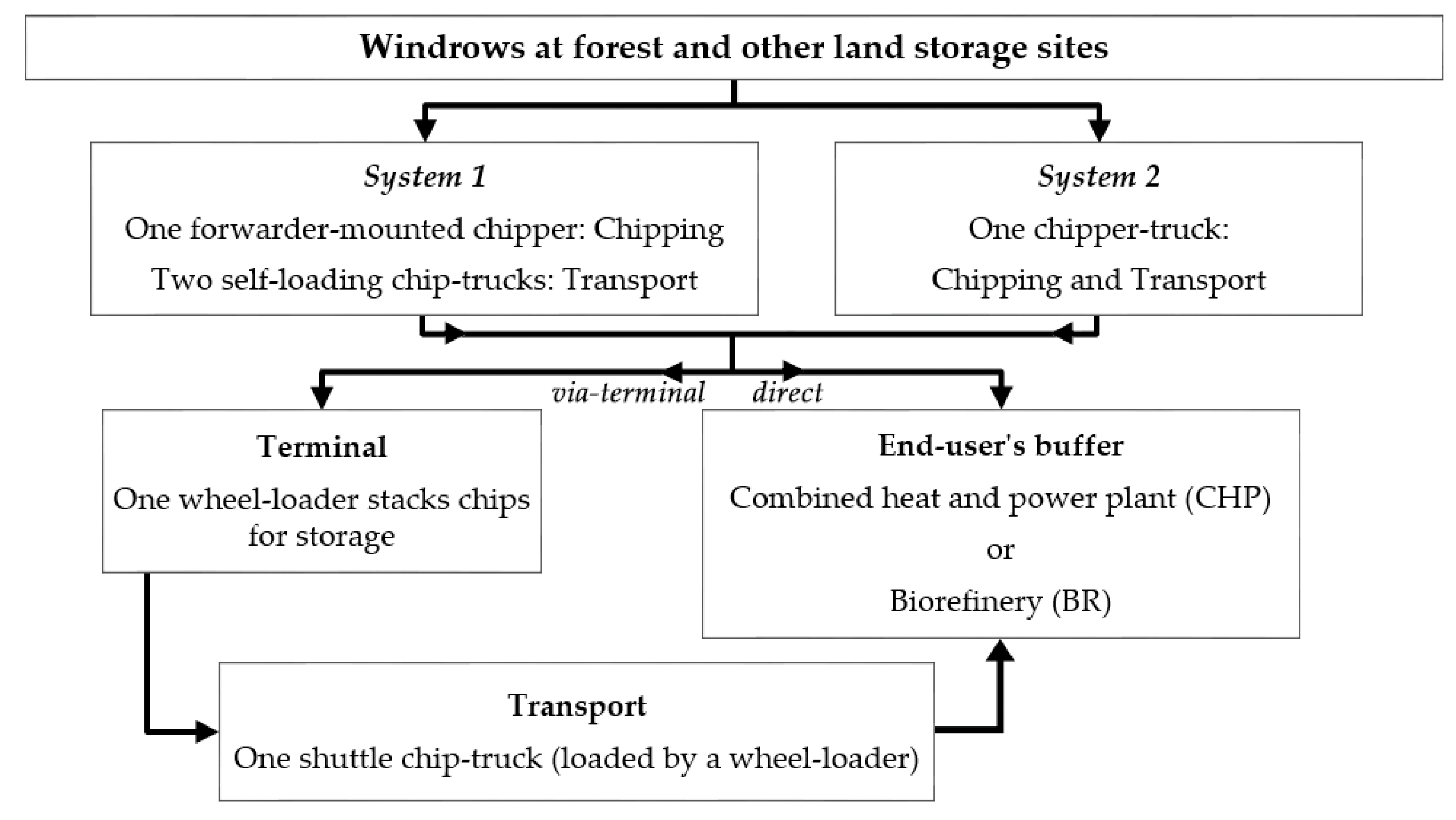
Figure 2.
Summary of the simulations’ main inputs and outputs.
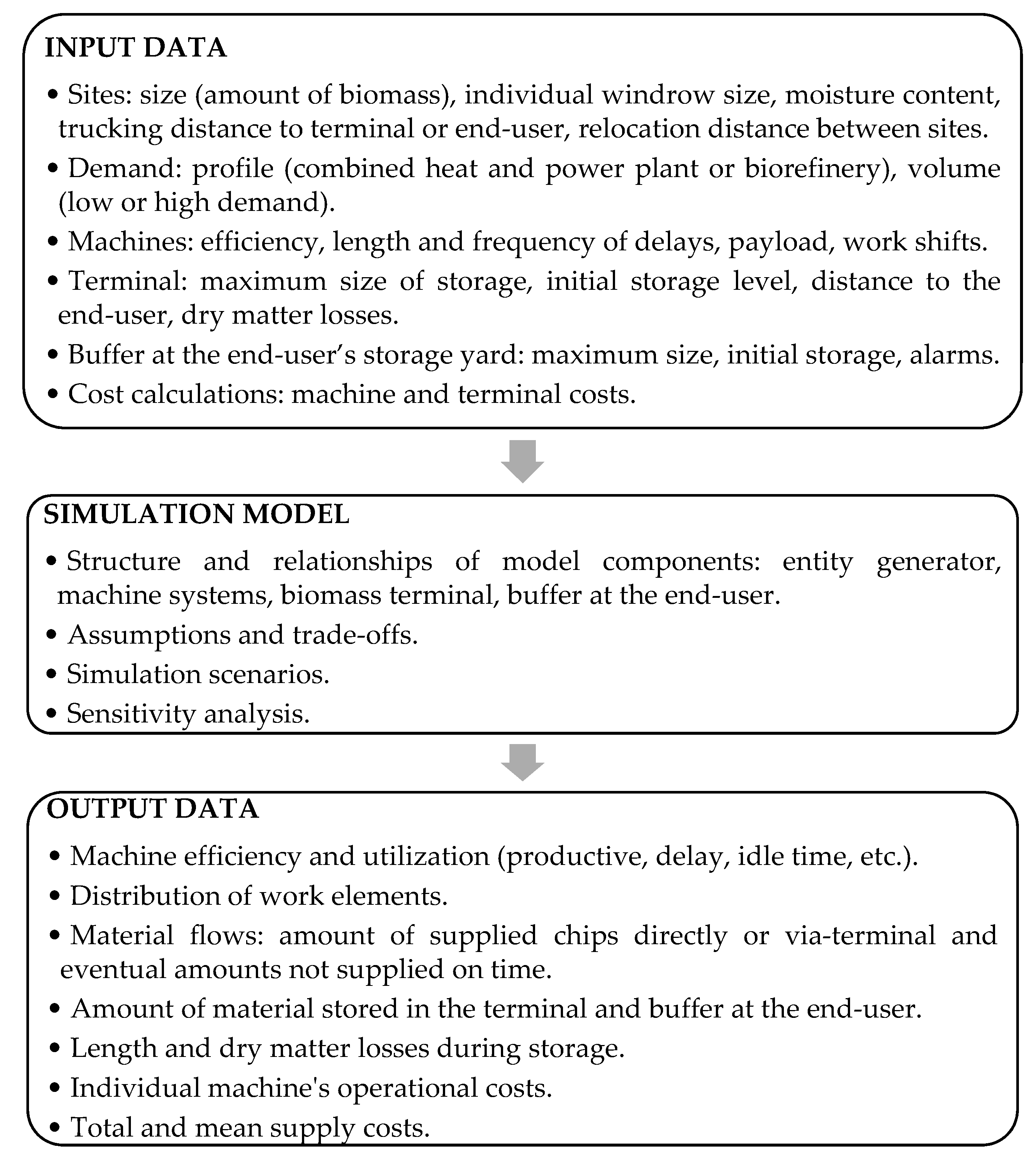
Figure 3.
Mean daily chip demand for each end-user (input values for high-demand scenarios).
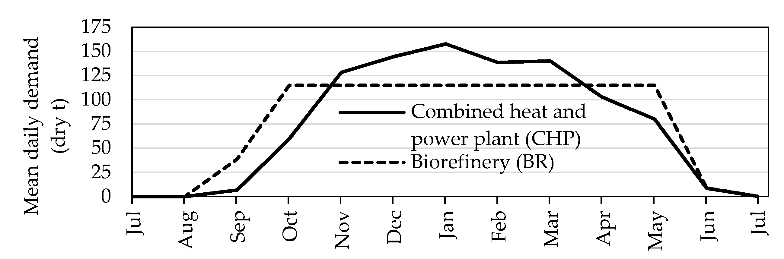
Figure 4.
Flowcharts of the logic of the work of terminal machinery.

Figure 5.
Flowcharts of the logic of the work of machines in System 1 and System 2.
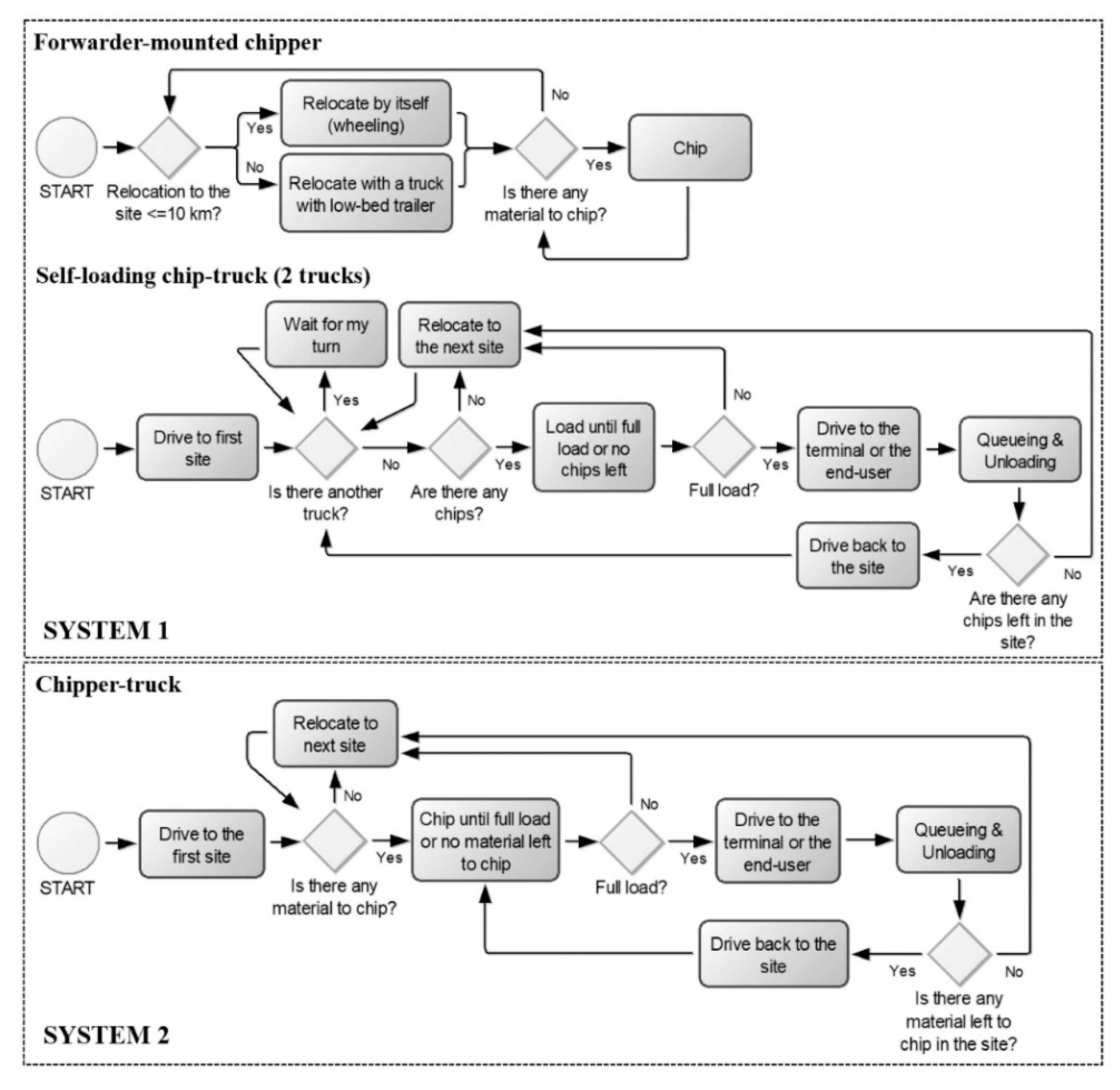
Figure 6.
Contributions of individual machines to the annual (total) supply cost.

Figure 7.
Mean actual use (%, spent SMh divided by available SMh) of machines in the simulation.
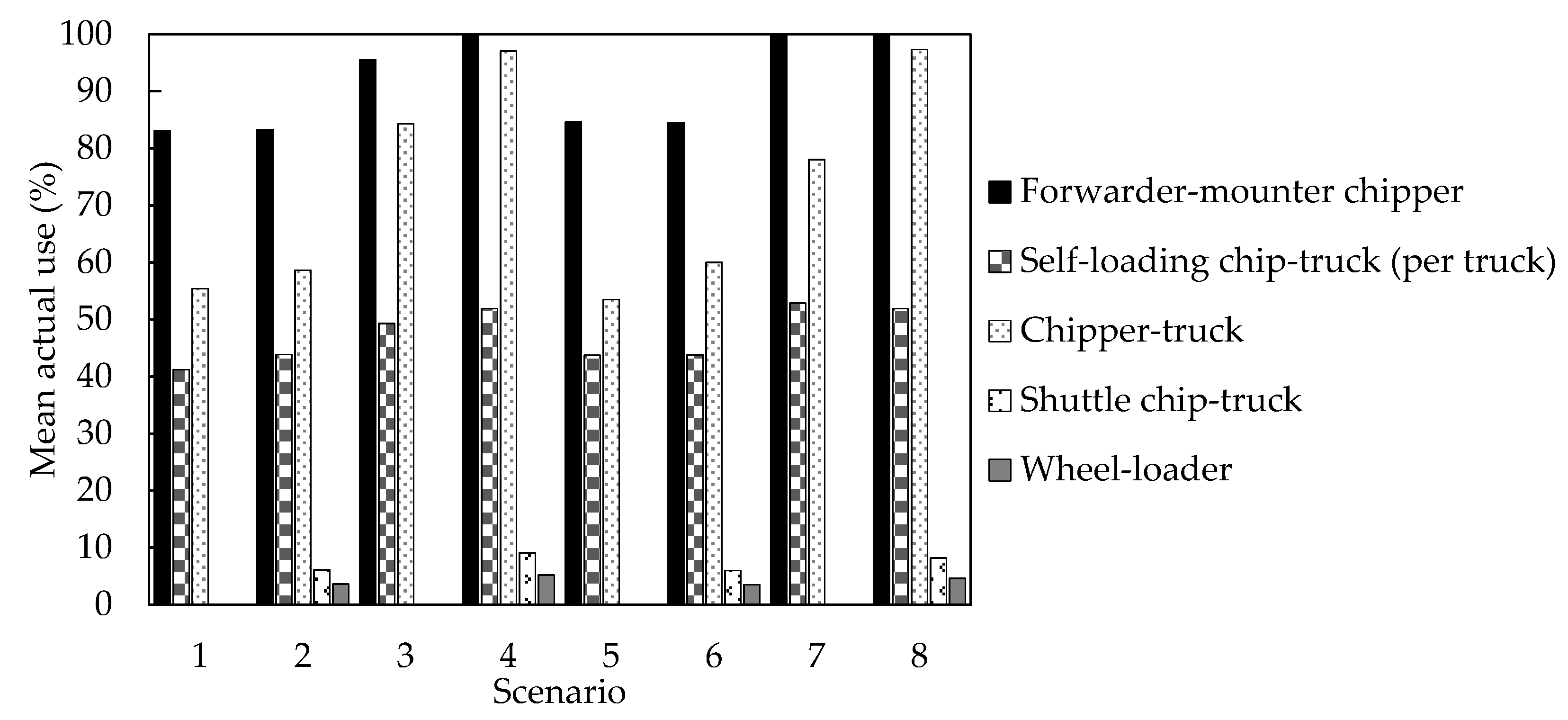
Figure 8.
Mean monthly production (dry t) of the supply fleet for direct (a) and combined chains (b) when supplying the combined heat and power plant (CHP) and biorefinery (BR) at the high-demand scenarios. FM = forwarder-mounted; SL = self-loading.
Figure 8.
Mean monthly production (dry t) of the supply fleet for direct (a) and combined chains (b) when supplying the combined heat and power plant (CHP) and biorefinery (BR) at the high-demand scenarios. FM = forwarder-mounted; SL = self-loading.

Figure 9.
Productive work time consumption (%, mean for all runs and scenarios) divided into work elements of the modelled forwarder-mounted chipper (a) and chipper-truck (b). Road transport for the chipper-truck entails relocation between sites and driving to/from the terminal or end-user.
Figure 9.
Productive work time consumption (%, mean for all runs and scenarios) divided into work elements of the modelled forwarder-mounted chipper (a) and chipper-truck (b). Road transport for the chipper-truck entails relocation between sites and driving to/from the terminal or end-user.
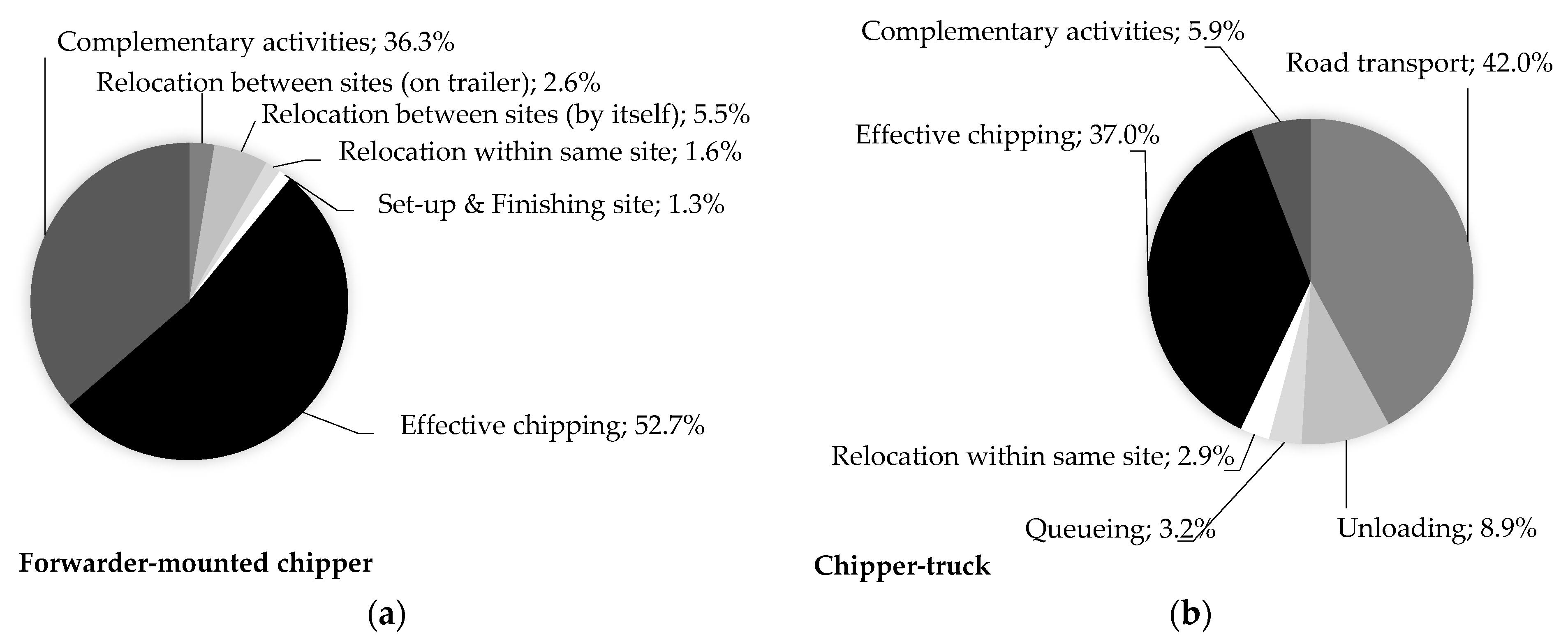
Figure 10.
Mean chip flow in/out of the terminal (weekly) and storage levels (daily) when supplying the combined heat and power plant (CHP) (a) and biorefinery (BR) (b) at the high-demand scenarios.
Figure 10.
Mean chip flow in/out of the terminal (weekly) and storage levels (daily) when supplying the combined heat and power plant (CHP) (a) and biorefinery (BR) (b) at the high-demand scenarios.

Table 1.
Attributes allocated to the generated entities, representative of sites in forest and other land containing LR and ST windrows as in [11]. To ease the interpretation of the distributions, the range of variation (around the median) of 95% of the measurements was determined.
Table 1.
Attributes allocated to the generated entities, representative of sites in forest and other land containing LR and ST windrows as in [11]. To ease the interpretation of the distributions, the range of variation (around the median) of 95% of the measurements was determined.
| Attributes | Unit | Distribution | 95% of Values between |
|---|---|---|---|
| Site size 1 | dry t | Gamma (12, 1.53, 44.6) 2 | 42–88 |
| Individual windrow size | dry t | Gamma (12, 3.43, 10.9) 3 | 30–55 |
| Moisture content (MC) | % | Triangular (26, 45, 61) 4 | 44–48 |
| Trucking distance from sites to the terminal or end-user 5 | |||
| May-November | km | Triangular (40, 49, 99) 4 | 45–54 |
| December-April | km | Triangular (4, 27, 35) 4 | 20–29 |
| Relocation distance between sites 6 | km | Beta (0.10, 68, 0.56, 4.83) 7 | 5–15 |
1 The number of windrows at a surveyed site ranged from 1 to 10; 2 Gamma (minimum, shape parameter, scale parameter), with an upper boundary of 350 dry t; 3 Gamma (minimum, shape parameter, scale parameter), with an upper boundary of 111 dry t; 4 Triangular (minimum, mode, maximum); 5 Observed trucking distances to a CHP during fieldwork. Distances were clustered into two groups: one for sites that were far from end-users (during the low heating season) and the other for sites close to end-users (during the high heating season). The distribution of trucking distances between the sites and terminal was assumed to be identical to that for distances between sites and end-users; 6 Distances were calculated based on the chipper’s routes observed during fieldwork. The routes were originally planned by the chip supplier; 7 Beta (minimum, maximum, lower shape parameter, upper shape parameter).
Table 2.
Main efficiency data (productive work time) of the modelled comminution equipment.
| Work Element | Unit | Description and Distribution | |
|---|---|---|---|
| Forwarder-Mounted Chipper | Chipper-Truck | ||
| Set-up at site | min | After relocation to new site: unload chains, tracks, portable wooden bridge and a log. | − |
| Triangular (2, 3, 6) 1 | |||
| Finishing site | min | Before relocation to new site: loading of elements in set-up. If road damages, the ground was flattened with a log and forwarder’s front-mounted shovel. | − |
| Triangular (2, 3, 6) 1 | |||
| Chipping | min dry t 1 | Chipping including crane work. | Chipping including crane work. |
| Triangular (2.3, 4.1, 6.1) 1 | Triangular (3.2, 4.8, 6.2) 1 | ||
| Complementary activities to chipping | min dry t 1 | Comprises terrain driving empty/full between the windrow-tipping point at the roadside and along the windrow, tipping over the chip-bin, engine start/shutdownometimes compaction of a snow surface for tipping chips over. | Comprises preparations: the driver changing cabin, eventual relocation along the windrow and engine start/shutdown. |
| Triangular (0.8, 2.0, 5.7) 1 | Triangular (0.6, 0.7, 0.9) 1 | ||
| Terrain driving for relocation within the site | min | Number of windrows: 2–6: Power Function (0,50, 0.77) 2 ≥7: Power Function (0,75, 0.77) 2 | Number of windrows: 2–6: Power Function (0,22, 0.77) 2 ≥7: Power Function (0,34, 0.77) 2 |
1 Triangular (minimum, mode, maximum); 2 Power Function (minimum, maximum, shape parameter).
Table 3.
Main specifications and efficiency data (productive work time) of the modelled transport vehicles.
Table 3.
Main specifications and efficiency data (productive work time) of the modelled transport vehicles.
| Variable | Unit | Chipper-Truck | Self-Loading Chip-Truck | Shuttle Chip-Truck |
|---|---|---|---|---|
| Cargo volume | m3 | 102 | 120 | 140 |
| Tare weight | tonnes | 33 | 30 | 22 |
| Payload | tonnes | 31 | 34 | 42 |
| Break-even moisture content (MC) | % | 46.1 | 42.6 | 45.8 |
| Work element | ||||
| Loading | min | − | Triangular (41, 53, 65) 1 | − |
| Unloading (incl. load measurement and MC sampling) | min | Triangular (14, 18, 23) 1 | Triangular (14, 18, 23) 1 | Triangular (14, 18, 23) 1 |
1 Triangular (minimum, mode, maximum).
Table 4.
Summary of main assumptions made when calculating machine hourly costs.
| Machine | Investment k€ | Useful life of Asset Years | Utilization Rate % | Cost € SMh−1 |
|---|---|---|---|---|
| Forwarder-mounted chipper | 547 | 5 | 89 | 159 |
| Chipper-truck | 640 | 5 | 95 | 181 |
| Self-loading chip-truck + trailer | 458 | 7 | 100 | 133 |
| Shuttle chip-truck + trailer | 372 | 7 | 100 | 119 |
| Wheel-loader | 208 | 5 | 95 | 55 |
Table 5.
Summary of main variables for calculating terminal operational cost.
| Variable | Unit | Value |
|---|---|---|
| Total terminal area | ha | 2 |
| Area devoted to storage | % | 90 |
| Area paved | % | 100 |
| Purchase price of land | € m−2 | 0.5 |
| Gravel paved cost | € m−2 | 30 |
| Depreciation time | year | 15 |
| Interest rate | % | 5.5 |
| Space utilization | dry t m−2 | 0.78 |
| Material turnover | times per year | 1.5 |
| Operational cost | € dry t−1 | 8.3 |
Table 6.
Simulated scenarios.
| End-User | Demand Volume | Supply Alternative | Scenario |
|---|---|---|---|
| Combined heat and power plant (CHP) | Low (21,000 dry t) | Direct (only) | 1 |
| Combined (direct and via-terminal) | 2 | ||
| High (29,000 dry t) | Direct (only) | 3 | |
| Combined (direct and via-terminal) | 4 | ||
| Biorefinery (BR) | Low (21,000 dry t) | Direct (only) | 5 |
| Combined (direct and via-terminal) | 6 | ||
| High (29,000 dry t) | Direct (only) | 7 | |
| Combined (direct and via-terminal) | 8 |
Table 7.
Mean and annual (total) supply cost of chips. Different superscripted lowercase letters indicate significant differences (p < 0.05) between scenarios (row-wise). Standard deviation (SD) in parentheses.
Table 7.
Mean and annual (total) supply cost of chips. Different superscripted lowercase letters indicate significant differences (p < 0.05) between scenarios (row-wise). Standard deviation (SD) in parentheses.
| End-User | Combined Heat and Power Plant (CHP) | Biorefinery (BR) | ||||||
|---|---|---|---|---|---|---|---|---|
| Demand | Low | High | Low | High | ||||
| Supply | Direct | Combined | Direct | Combined | Direct | Combined | Direct | Combined |
| Scenario | 1 | 2 | 3 | 4 | 5 | 6 | 7 | 8 |
| Mean cost (€ dry t−1) | 43.0 d,e (0.7) | 47.8 a (0.4) | 42.4 e (0.1) | 46.2 b (0.2) | 44.0 c (0.6) | 48.2 a (0.2) | 43.6 c,d (0.2) | 45.8 b (0.3) |
| Annual cost (k€) | 914 a (10) | 1004 b (9) | 1161 c (11) | 1340 d (4) | 929 e (5) | 1014 b (3) | 1184 f (6) | 1335 d (3) |
Table 8.
Mean operational cost and productivity of machinery (all runs and scenarios, SD in parentheses), including relocations. Productive machine hours (PMh) refer to machine working time excluding delays.
Table 8.
Mean operational cost and productivity of machinery (all runs and scenarios, SD in parentheses), including relocations. Productive machine hours (PMh) refer to machine working time excluding delays.
| Cost € Dry t−1 | Overall Productivity Dry t PMh−1 | Productivity Only Chipping Dry t PMh−1 | |
|---|---|---|---|
| Forwarder-mounted chipper | 23.8 (0.3) | 7.7 (0.1) | 14.4 (0.2) |
| Self-loading chip-truck (per truck) | 20.4 (0.4) | 6.5 (0.1) | − |
| Chipper-truck | 40.8 (1.2) | 4.7 (0.1) | 12.5 (0.1) |
| Shuttle chip-truck | 6.5 (0.1) | 18.2 (0.3) | − |
| Wheel-loader | 0.8 (0.0) | 71.9 (1.6) | − |
| Terminal operation | 8.3 (0.0) | − | − |
Table 9.
Annual material flows with mean amount of chips supplied directly, via-terminal and missing (i.e., not supplied on time to fulfil demand) for each scenario (SD in parentheses).
Table 9.
Annual material flows with mean amount of chips supplied directly, via-terminal and missing (i.e., not supplied on time to fulfil demand) for each scenario (SD in parentheses).
| End-User | Demand | Supply | Scenario | Annual Material Flows | ||||||
|---|---|---|---|---|---|---|---|---|---|---|
| Direct | Via-Terminal | Missing | Sum Supplied | |||||||
| Dry t | % | Dry t | % | Dry t | % | Dry t | ||||
| CHP | Low | Direct | 1 | 21,272 (290) | 100 | − | − | 0 | 0 | 21,272 (290) |
| CHP | Low | Combined | 2 | 17,713 (56) | 84 | 3293 (73) | 16 | 0 | 0 | 21,006 (41) |
| CHP | High | Direct | 3 | 27,413 (192) | 92 | − | − | 2289 (282) | 8 | 27,413 (192) |
| CHP | High | Combined | 4 | 24,100 (280) | 83 | 4927 (129) | 17 | 0 | 0 | 29,027 (159) |
| BR | Low | Direct | 5 | 21,087 (351) | 100 | − | − | 0 | 0 | 21,087 (351) |
| BR | Low | Combined | 6 | 17,764 (47) | 84 | 3259 (107) | 16 | 0 | 0 | 21,023 (87) |
| BR | High | Direct | 7 | 27,158 (108) | 92 | − | − | 2483 (167) | 8 | 27,158 (108) |
| BR | High | Combined | 8 | 24,662 (95) | 85 | 4486 (97) | 15 | 0 | 0 | 29,148 (116) |
Table 10.
Mean storage time, storage levels and annual dry matter losses at the terminal (SD in parentheses).
Table 10.
Mean storage time, storage levels and annual dry matter losses at the terminal (SD in parentheses).
| End-User | Demand | Scenario | Mean Storage Time | Mean Storage Levels | Annual Dry Matter Losses | |
|---|---|---|---|---|---|---|
| Weeks | dry t | dry t | % of Annual Supply | |||
| CHP | Low | 2 | 28 (0.5) | 2095 (18) | 547 (16) | 2.5 |
| CHP | High | 4 | 15 (0.9) | 1563 (129) | 400 (20) | 1.4 |
| BR | Low | 6 | 27 (0.5) | 1998 (35) | 488 (24) | 2.3 |
| BR | High | 8 | 12 (0.6) | 1182 (66) | 279 (12) | 0.9 |
Table 11.
Mean supply cost (€ dry t−1) in sensitivity analyses. Deviations from the reference cost for scenarios 3, 4, 7 and 8 are shown in parentheses. Reference trucking distances are specified in Table 1.
Table 11.
Mean supply cost (€ dry t−1) in sensitivity analyses. Deviations from the reference cost for scenarios 3, 4, 7 and 8 are shown in parentheses. Reference trucking distances are specified in Table 1.
| Scenario | Reference Cost | 25% Longer Trucking Distances | 50% Longer Trucking Distances | Low Integration (50% Longer Relocations) | High Integration (50% Shorter Relocations) |
|---|---|---|---|---|---|
| 3 | 42.2 | 44.9 (+6.0%) | 46.9 (+10.7%) | 43.2 (+1.9%) | 41.8 (−1.4%) |
| 4 | 46.2 | 48.2 (+4.3%) | 51.2 (+11.0%) | 47.1 (+2.0%) | 45.2 (−2.1%) |
| 7 | 43.6 | 45.8 (+5.0%) | 48.1 (+10.4%) | 44.4 (+1.7%) | 42.7 (−2.1%) |
| 8 | 45.8 | 48.3 (+5.3%) | 50.5 (+10.2%) | 46.6 (+1.8%) | 45.2 (−1.3%) |
Table 12.
Mean machine operational cost (€ dry t−1) in sensitivity analyses. Deviations from the reference cost for scenarios 3, 4, 7 and 8 are shown in parentheses.
Table 12.
Mean machine operational cost (€ dry t−1) in sensitivity analyses. Deviations from the reference cost for scenarios 3, 4, 7 and 8 are shown in parentheses.
| Machine (Common for Scenarios 3, 4, 7, 8) | Reference Cost | 25% Longer Trucking Distances | 50% Longer Trucking Distances | Low Integration (50% Longer Relocations) | High Integration (50% Shorter Relocations) |
|---|---|---|---|---|---|
| Forwarder-mounted chipper | 23.7 | − | − | 24.5 (+3.6%) | 22.7 (−3.9%) |
| Self-loading chip-truck | 20.4 | 22.3 (+9.7%) | 24.2 (+19.1%) | − | − |
| Chipper-truck | 40.2 | 43.4 (+7.9%) | 46.2 (+15.0%) | 40.4 (+0.5%) | 40.1 (−0.3%) |
© 2019 by the authors. Licensee MDPI, Basel, Switzerland. This article is an open access article distributed under the terms and conditions of the Creative Commons Attribution (CC BY) license (http://creativecommons.org/licenses/by/4.0/).
Share and Cite
MDPI and ACS Style
Fernandez-Lacruz, R.; Eriksson, A.; Bergström, D. Simulation-Based Cost Analysis of Industrial Supply of Chips from Logging Residues and Small-Diameter Trees. Forests 2020, 11, 1. https://doi.org/10.3390/f11010001
AMA Style
Fernandez-Lacruz R, Eriksson A, Bergström D. Simulation-Based Cost Analysis of Industrial Supply of Chips from Logging Residues and Small-Diameter Trees. Forests. 2020; 11(1):1. https://doi.org/10.3390/f11010001
Chicago/Turabian StyleFernandez-Lacruz, Raul, Anders Eriksson, and Dan Bergström. 2020. "Simulation-Based Cost Analysis of Industrial Supply of Chips from Logging Residues and Small-Diameter Trees" Forests 11, no. 1: 1. https://doi.org/10.3390/f11010001
Note that from the first issue of 2016, this journal uses article numbers instead of page numbers. See further details here.