The Smallest Grammar Problem as Constituents Choice and Minimal Grammar Parsing

Abstract
: The smallest grammar problem—namely, finding a smallest context-free grammar that generates exactly one sequence—is of practical and theoretical importance in fields such as Kolmogorov complexity, data compression and pattern discovery. We propose a new perspective on this problem by splitting it into two tasks: (1) choosing which words will be the constituents of the grammar and (2) searching for the smallest grammar given this set of constituents. We show how to solve the second task in polynomial time parsing longer constituent with smaller ones. We propose new algorithms based on classical practical algorithms that use this optimization to find small grammars. Our algorithms consistently find smaller grammars on a classical benchmark reducing the size in 10% in some cases. Moreover, our formulation allows us to define interesting bounds on the number of small grammars and to empirically compare different grammars of small size.1. Introduction
The smallest grammar problem—namely, finding a smallest context-free grammar that generates exactly one sequence—is of practical and theoretical importance in fields such as Kolmogorov complexity, data compression and pattern discovery.
The size of a smallest grammar can be considered a computable variant of Kolmogorov complexity, in which the Turing machine description of the sequence is restricted to context-free grammars. The problem is then decidable, but still hard: the problem of finding a smallest grammar with an approximation ratio smaller than
is NP-HARD [1]. Nevertheless, a
 (log3 n) approximation ratio—with n the length of the sequence—can be achieved by a simple algorithmic scheme based on an approximation to the shortest superstring problem [1] and a smaller
(log n/g) (where g is the size of a smallest grammar) approximation ratio is possible through more complex mappings from the LZ77-factorization of the sequence to a context-free grammar with a balanced parsing tree [1,2].
(log3 n) approximation ratio—with n the length of the sequence—can be achieved by a simple algorithmic scheme based on an approximation to the shortest superstring problem [1] and a smaller
(log n/g) (where g is the size of a smallest grammar) approximation ratio is possible through more complex mappings from the LZ77-factorization of the sequence to a context-free grammar with a balanced parsing tree [1,2].
If the grammar is small, storing the grammar instead of the sequence can be interesting from a data compression perspective. Kieffer and Yang developed the formal framework of compression by Grammar Based Codes from the viewpoint of information theory, defining irreducible grammars and demonstrating their universality [3]. Before this formalization, several algorithms allowing to compress a sequence by context-free grammars had already been proposed. The LZ78-factorization introduced by Ziv and Lempel in [4] can be interpreted as a context-free grammar. Let us remark that this is not true for LZ77, published one year before [5]. Moreover, it is a commonly used result that the size of a LZ77-factorization is a lower bound on the size of a smallest grammar [1,2]. The first approach that generated explicitly a context-free grammar with compression ability is Sequitur [6]. Like LZ77 and LZ78, Sequitur is an on-line algorithm that processes the sequence from left to right. It incrementally maintains a grammar generating the part of the sequence read, introducing and deleting production to ensure that no digram (pair of adjacent symbols) occurs more than once and that each rule is used at least twice. Other algorithms consider the entire sequence before choosing which repeated substring will be rewritten by the introduction of a new rule. Most of these offline algorithms proceed in a greedy manner, selecting in each iteration one repeated word w according to a score function and replacing all the (non-overlapping) occurrences of the repeat w in the whole grammar by a new terminal N and adding the new production N → w to the grammar. Different heuristics have been used to choose the repeat: the most frequent one [7], the longest [8] and the one that reduces the most the size of the resulting grammar (Compressive [9]). Greedy [10] belongs to this last family but the score used for choosing the words is oriented toward directly optimizing the number of bits needed to encode the grammar rather than minimizing its size. The running time of Sequitur is linear and linear-time implementations of the first two algorithms exists: RePair [11] and Longest First [12], while the existence of a linear-time algorithm for Compressive and Greedy remains an open question.
In pattern discovery, a smallest grammar is a good candidate for being the one that generates the data according to Occam's razor principle. In that case, the grammar may not only be used for compressing the sequence but also to unveil its structure. Inference of the hierarchical structure of sequences was the initial motivation of Sequitur and has been the subject of several papers applying this scheme to DNA sequences [6,13,14], musical scores [15] or natural languages [7,16]. It can also be a first step to learn more general grammars along the lines of [17]. In all the latter cases, a slight difference in the size of the grammar, which would not matter for data compression, can dramatically change the results with respect to the structure. Thus, more sophisticated algorithms than those for data compression are needed.
In this article, which is an extended version of [18], we focus on how to choose occurrences that are going to be rewritten. This issue was generally handled straightforwardly in former algorithms by selecting all the non-overlapping occurrences in a left to right order. Moreover, once an occurrence had been chosen for being rewritten, the result was definitive and was not altered by the words chosen in the following iterations. In order to remedy these flaws, we show how to globally optimize the choice of the occurrences to be replaced by non-terminals. We are then able to improve classical greedy algorithms by introducing this optimization step at each iteration of the algorithm. This optimization allows us to define the smallest grammar problem in terms of two complementary optimization problems: the choice of non-terminals and the choice of their occurrences. We redefine the search space, prove that all solutions are contained in it and propose a new algorithm performing a wider search by adding the possibility to discard non-terminals previously included in the grammar. Thanks to our new formulation, we are able to analyze the number of different grammars with the same minimal size and present empirical results that measure the conservation of structure among them.
The outline of this paper is the following: in Section 2 we formally introduce the definitions and in Section 3 the classical offline algorithms. Section 4 contains our main contributions. In Section 4.1 we show how to optimize the choice of occurrences to be replaced by non-terminals for a set of words and then extend offline algorithms by optimizing the choice of the occurrences at each step in Section 4.2. We present our search space and show that this optimization can also be used directly to guide the search in a new algorithm in Section 4.3. We present experiments on a classical benchmark in Section 5 showing that the occurrence optimization consistently allows to find smaller grammars. In Section 6 we consider the number of smallest grammars that may exist and discuss the consequences of our results on structure discovery.
2. Previous work and definitions
2.1. Definitions and Notation
We start by giving a few definitions and setting up the nomenclature that we use along the paper. A string s is a sequence of characters s1 … sn, its length, |s| = n. ∊ denotes the empty string, and s[i : j] = si … sj, s[i : j] = ∊ if j < i. We say that a word w occurs at position i, if w = s[i : i + |w| − 1]. w is a repeat of s if it occurs more than once in s and |w| > 1. We denote by repeats(s) the set of substrings of s that occur more than once and of length greater than one. For example repeats(abaaab) = {ab, aa} and aa occurs at position 2 and 3.
A context-free grammar is a tuple 〈Σ,
 ,
,
 , S〉, where Σ is the finite set of terminals and
the finite set of non-terminals,
and Σ disjoint. S ∈
is called the start symbol and
is the set of productions. Each production (also called rule) is of the form A → α where its left-hand side A is a non-terminal and its right-hand side α belongs to (Σ ∪
)*. We say
, if α is of the form δCδ′, β = δγδ′ and C → γ is a production. A sequence
is called a derivation and in this case we say that α produces β and that β derives from α (denoted by α ⇒ β).
, S〉, where Σ is the finite set of terminals and
the finite set of non-terminals,
and Σ disjoint. S ∈
is called the start symbol and
is the set of productions. Each production (also called rule) is of the form A → α where its left-hand side A is a non-terminal and its right-hand side α belongs to (Σ ∪
)*. We say
, if α is of the form δCδ′, β = δγδ′ and C → γ is a production. A sequence
is called a derivation and in this case we say that α produces β and that β derives from α (denoted by α ⇒ β).
Given a string α over (
∪ Σ)*, its constituents (cons(α)) are the possible strings of terminals that can be derived from α. Formally, cons(α) = {w ∈ Σ* : α ⇒ w}. The constituents of a grammar are all the constituents of its non-terminals. The language is the set of constituents of the start symbol S, cons(S).
Because the Smallest Grammar framework seeks for a context-free grammar whose language contains one and only one string, the grammars we consider here neither branch (every non-terminal occurs at most once as a left-hand side of a rule) nor loop (if B occurs in any derivation starting with A, then A will not occur in a derivation starting with B). In this type of grammars, any substring of the grammar has a unique constituent, in which case we will drop the set notation and define cons(α) as the only terminal string that can be derived from α. Note that if the grammar is in Chomsky Normal Form [19], it is equivalent to a straight-line program.
Several definitions of the grammar size exist. Following [9], we define the size of the grammar G, denoted by |G|, to be the length of its encoding by concatenation of its right-hand sides separated by end-of-rule markers: |G| =ΣA→α∈
 (|α| + 1).
3. IRR
3.1. General Scheme
Most offline algorithms follow the same general scheme. First, the grammar is initialized with a unique initial rule S → s where s is the input sequence and then they proceed iteratively. At each iteration, a word ω occurring more than once in s is chosen according to a score function f, all the (non-overlapping) occurrences of ω in the grammar are replaced by a new non-terminal Nω and a new production Nω → ω is added to the grammar. We give pseudo-code for this general scheme that we name Iterative Repeat Replacement (IRR) in Algorithm 1. There,
is the set of production rules being built: this defines a unique grammar G(
) and therefore we define |
| = |G(
)|. The set of repeats of size longer than one of the right-hand sides of
is denoted by repeats(
) and
ω↦N is the result of the substitution of ω by the new symbol N in the right-hand sides of
as detailed in the next paragraph.
When occurrences overlap, one has to specify which occurrences have to be replaced. One solution is to choose all the elements in the canonical list of non-overlapping occurrences of ω in s, which we define to be the list of non-overlapping occurrences of ω in a greedy left to right way (all occurrences overlapping with the first selected occurrence are not considered, then the same thing with the second non-eliminated occurrence, etc.). This ensures that a maximal number of occurrences will be replaced. When searching for the smallest grammar, one has to consider not only the occurrences of a word in s but also their occurrence in right-hand sides of rules that are currently part of the grammar. A canonical list of non-overlapping occurrences of ω can be defined for each right-hand side appearing in the set of production rules
. This provides a straightforward list of occurrences used in the scoring function or the replacement step by our pseudo-code defining IRR.
The IRR schema instantiates different algorithms, depending on the score function f(ω,
) it uses. Longest First corresponds to f(ω,
) = fML(ω,
) = |ω|. Choosing the most frequent repeat, like in RePair, corresponds to use f(ω,
) = fMF(ω,
) = o (ω), where o (ω) is the length of the canonical non-overlapping list of ω in the right-hand sides of rules in
. Note however the difference that IRR is more general than RePair and may select a word which is not a digram.
In order to derive a score function corresponding to Compressive, note that replacing a word ω by a non-terminal results in a contraction of the grammar of (|ω| − 1)*o (ω) and its inclusion in the grammar adds |ω| + 1 to the grammar size. This defines f(ω,
) = fMC(ω,
) = (|ω| − 1)*(o (ω) − 1) − 2. We call these three algorithms IRR-ML (maximal length), IRR-MF (most frequent) and IRR-MC (maximal compression), respectively.
| Algorithm 1 Iterative Repeat Replacement. | |
| IRR(s, f) | |
| Require: s is a sequence, and f is a score function | |
| 1: | ← {Ns → s} |
| 2: | while ∃ω : ω ← argmaxα∈repeats(
) f(α,
) ∧ |
ω↦Nω| < |
| do |
| 3: |
←
ω←Nω ∪ {Nω → ω} |
| 4: | end while |
| 5: | return G(
) |
The complexity of IRR when it uses one of these scores is
(n3) since for a sequence of size n, the computation of the scores involving only o (ω) and |ω| of the
(n2) possible repeats can be done in
(n2) using a suffix tree structure [20] and the number of iterations is bounded by n since the size of the grammar strictly decreases at each step.
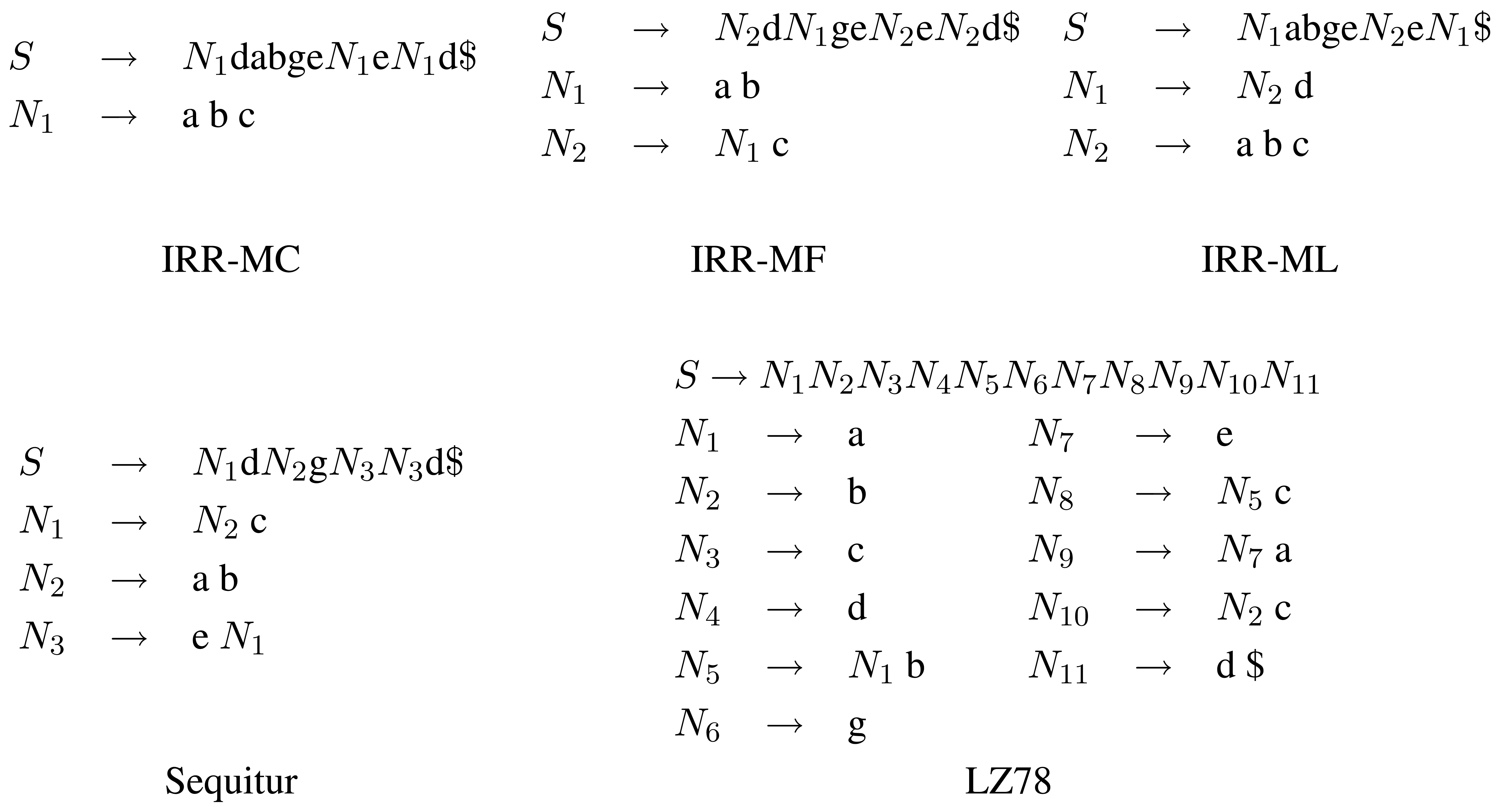
The grammars found by the three IRR algorithms, plus Sequitur and LZ78 are shown on a small example in Figure 1. A comparison of the size of the grammars returned by these algorithms over a standard data compression corpus are presented in Section 5. These results confirm that IRR-MC finds the smallest grammars as was suggested in [9]. Until now, no other polynomial time algorithm (including theoretical algorithms that were designed to achieve a low approximation ratio [1,2,21]) has proven (theoretically nor empirically) to perform better than IRR-MC.
3.2. Limitations of IRR
Even though IRR algorithms are the best known practical algorithms for obtaining small grammars, they present some weaknesses. In the first place, their greedy strategy does not guarantee that the compression gain introduced by a selected word ω will still be interesting in the final grammar. Each time an iteration selects a substring of ω, the length of the production rule is reduced; and each time a superstring is selected, its number of occurrences is reduced. Moreover, the first choices mark some breaking points and future words may appear inside them or in another parts of the grammar, but never span over these breaking points.
It could be argued that there may exist a score function that for every sequence scores the repeats in such a way that the order they are presented to IRR results in a smallest grammar. The following theorem proves that this is not the case.
Theorem 1
There are infinitely many sequences sk, over a constant alphabet, such that for any score function f, |IRR(sk, f)| is greater than the size of a smallest grammar for sk.
Proof
Consider the infinite set of sequences
Note that Theorem 1 does not make any assumptions over the possible score function f (like, for example, polynomial running time). In order to find G*, the choice of occurrences that will be rewritten should be flexible when considering repeats introduced in future iterations.
4. Choice of Occurrences
4.1. Global Optimization of Occurrences Replacement
Once an IRR algorithm has chosen a repeated word ω, it replaces all non-overlapping occurrences of that word in the current grammar by a new non-terminal N and then adds N → ω to the set of production rules. In this section, we propose to perform a global optimization of the replacement of occurrences, considering not only the last non-terminal but also all the previously introduced non-terminals. The idea is to allow occurrences of words to be kept (instead of being replaced by non-terminals) if replacing other occurrences of words overlapping them results in a better compression.
We propose to separate the choice of which terminal strings will be final constituents of the final grammar from the choice of which of the occurrences of these constituents will be replaced by non-terminals. First, let us assume that a set of constituents {s} ∪ Q is given and we want to find a smallest grammar whose constituent set is {s} ∪ Q. If we denote this set by {s = ω0, ω1, …, ωm}, we need to be able to generate these constituents and for each constituent ωi the grammar must thus have a non-terminal Ni such that ωi = cons(Ni). In the smallest grammar problem, no unnecessary rule should be introduced since the grammar has to generate only one sequence. More precisely such a grammar must have exactly m + 1 non-terminals and associate production rules.
For this, we define a new problem, called Minimal Grammar Parsing (MGP) Problem. An instance of this problem is a set of strings {s} ∪ Q, such that all strings of Q are substrings of s. A Minimal Grammar Parsing of {s} ∪ Q is a context-free grammar G = 〈Σ,
,
, S〉 such that:
all symbols of s are in Σ.
S derives only s.
for each string ωℓ {s} ∪ Q there is a non-terminal Nℓ that derives only ωℓ and
![Algorithms 04 00262i2]() = {N0 … Nm}.
= {N0 … Nm}.for each non-terminal N there is a string s′ of {s} ∪ Q such that N derives s′.
|G| is of minimal size for all possible grammars that satisfy conditions 1–4.
Note that this is similar to the Smallest Grammar Problem, except that all constituents for the non-terminals of the grammar are also given. The MGP problem is related to the problem of static dictionary parsing [22] with the difference that the dictionary also has to be parsed. This recursive approach is partly what makes grammars interesting to both compression and structure discovery.
As an example consider the sequence s = ababbababbabaabbabaa and suppose the constituents are {s, abbaba, bab}. This defines the set of non-terminals {N0, N1, N2}, such that cons(N0) = s, cons(N1) = abbaba and cons(N2) = bab. A minimal parsing is N0 → aN2N2N1N1a, and N1 → abN2a, N2 → bab.
This problem can be solved in a classical way in polynomial time by searching for a shortest path in |Q| + 1 graphs as follows. Given the set of constituents, s = {ω0, ω1, …, ωm}.
Let {N0, N1, …, Nm} be the set of non-terminals. Each Nℓ will be the non-terminal whose constituent is ωℓ.
Define m + 1 directed acyclic graphs Γ0 … Γm, where Γℓ = 〈Mℓ, Eℓ〉. If |ωℓ| = k then the graph Γℓ will have k + 1 nodes: Mℓ = {1 … |ωℓ| + 1}. The edges El are of two types:
for every node i there is an edge to node i + 1 labeled with ωℓ[i].
there will be an edge from node i to j + 1 labeled by Nm if there exists a non-terminal Nm different from Nℓ such that ωℓ[i : j] = ωm.
For each Γℓ, find a shortest path from 1 to |ωℓ| + 1.
Return the labels of these paths.
The right-hand side for non-terminal Nℓ is the concatenation of the labels of a shortest path of Γℓ. Intuitively, an edge from node i to node j + 1 with label Nm represents a possible replacement of the occurrence ωℓ[i : j] by Nm. There may be more than one grammar parsing with minimal size. If Q is a subset of the repeats of the sequence s, we denote by mgp({s} ∪ Q) the set of production rules
corresponding to one of the minimal grammar parsing of {s} ∪ Q.
The list of occurrences of each constituent over the original sequence can be stored at the moment it is chosen. Supposing then that the graphs are created, and as the length of each constituent is bounded by n = |s|, the complexity of finding a shortest path for one graph with a classical dynamic programming algorithm lies in
(n × m). Because there are m + 1 graphs, computing mgp({s} ∪ Q) is in
(n × m2).
Note that in practice the graph Γ0 contains all the information for all other graphs: any Γℓ is a subgraph of Γ0. Therefore, we call Γ0 the Grammar Parsing graph (GP-graph).
4.2. IRR with Occurrence Optimization
We can now define a variant of IRR, called Iterative Repeat Choice with Occurrence Optimization (IRCOO) whose pseudo-code is given in Algorithm 2. Different from IRR, what is maintained is a set of terminal strings, and the current grammar in each moment is a Minimal Grammar Parsing over this set of strings. Recall that cons(ω) gives the only terminal string that can be derived from ω (the “constituent”). Again, we define IRCCO-MC, IRCOO-MF, IRCOO-ML the instances of Algorithm 2 where the score function is defined as fMC, fMF, fML.
The computation of the argmax function depends only on the number of repeats, assuming that f is constant, so that its complexity lies in
(n2). Like for IRR, the total number of times the while loop is executed is bounded by n. The complexity of this generic scheme is thus
(n × (n2 + n × m2)).
| Algorithm 2 Iterative Repeat Choice with Occurrences Optimization. | |
| IRCOO(s, f) | |
| Require: s is a sequence, and f is a score function on words | |
| 1: |  ← {s} ← {s} |
| 2: | ← {S → s} |
| 3: | while (∃ω : ω ← argmaxα∈repeats(
) f(α,
)) ∧ |mgp(
∪ {cons(ω)})| < |
| do |
| 4: |
←
∪ {cons(ω)} |
| 5: |
← mgp(
) |
| 6: | end while |
| 7: | return G(
) |
As an example, consider again the sequence from Section 3.2, where α, β and γ have length one. After three iterations of IRRCOO-MC the words xax, xbx and xcx are chosen, and a MGP of these words plus the original sequence results in G*.
IRRCOO extends IRR by performing a global optimization at each step of the replaced occurrences but still relies on the classical score functions of IRR to choose the words to introduce. But the result of the optimization can be used directly to guide the search in a hill-climbing approach that we introduce in the next subsection.
4.3. Widening the Explored Space
In this section we divert from IRR algorithms by taking the idea presented in IRRCOO a step forward. Here, we consider the optimization procedure (mgp) as a scoring function for sets of substrings.
We first introduce the search space, defined over all possible sets of substrings, for the Smallest Grammar Problem and, second, an algorithm performing a wider exploration of this search space than the classical greedy methods.
4.3.1. The Search Space
The mgp procedure permits us to resolve the problem of finding a smallest grammar given a fixed set of constituents. The Smallest Grammar Problem reduces then to find this good set of constituents. This is the idea behind the search space we will consider here.
Consider the lattice 〈(s), ⊆〉, where (s) is the collection of all possible sets of repeated substrings in s: (s) = 2repeats(s). Every node of this lattice corresponds to a set of repeats of s. We then define a score function over the nodes of the lattice as score(η) = |mgp({s} ∪ η)|.
An algorithm over this search space will look for a local or global minimum. To define this, we first need some notation:
Definition 1
Given a lattice 〈L, ⪯〉:
ancestors(η) = {θ ≠ η | η ⪯ θ ∧ (∄κ, κ ≠ η,θ s.t. η ⪯ κ ⪯ θ)}
descendants(η) = {θ ≠ η | θ ⪯ η ∧ (∄κ, κ ≠ η,θ s.t. θ ⪯ κ ⪯ η)}
The ancestors of node η are the nodes exactly “over” η, while the descendants of node η are the nodes exactly “under” η.
Now, we are able to define a global and local minimum.
Definition 2
Given a lattice 〈L, ⪯〉 and an associate score function over nodes, g(η):
A node η is a global minimum if g(η) ≤ g(θ) for all θ ∈ L.
A node η is a local minimum if g(η) ≤ g(θ) for all θ ∈ ancestors(η) ∪ descendants(η).
Unless otherwise noted the default score function for nodes will be score(η) (defined above). Finally, let

 (s) be the set of all grammars of minimal size for the sequence s. Similarly, we define
({s} ∪ η) the set of minimal grammars with constituents {s} ∪ η. With this definition, we can state formally that this lattice is a “good” search space:
(s) be the set of all grammars of minimal size for the sequence s. Similarly, we define
({s} ∪ η) the set of minimal grammars with constituents {s} ∪ η. With this definition, we can state formally that this lattice is a “good” search space:
Theorem 2
Proof
To see the first inclusion (⊆), take a smallest grammar G*. All strings in cons(G*) have to be repeats of s, so cons(G*)\{s} corresponds to a node η in the lattice and G* has to be in
({s} ∪ η). Conversely (⊇), all grammars of the right expression have the same size, which is minimal, so they are all smallest grammars.
Because of the NP-hardness of the problem, it is fruitless (supposing P ≠ NP) to search for an efficient algorithm to find a global minimum. We will present therefore an algorithm that looks for a local minimum on this search space.
4.3.2. The Algorithm
In contrast with classical methods, we can now define algorithms discarding also constituents. To perform a wider exploration of the search space, we propose a new algorithm performing a succession of greedy search in ascending and descending directions in the lattice until a local minimum is found.
This algorithm explores the lattice in a zigzag path. Therefore we denote it ZZ. It explores the lattice by an alternation of two different phases: bottom-up and top-down. The bottom-up can be started at any node, it moves upwards in the lattice and at each step it looks among its ascendants for the one with the lowest score. In order to determine which is the one with the lowest score, it inspects them all. It stops when no ascendant has a better score than the current one. As in bottom-up, top-down starts at any given node but it moves downwards looking for the node with the smallest score among its descendants. Going up or going down from the current node is equivalent to adding or removing a substring to or from the set of substrings in the current node respectively.
ZZ starts at the bottom node, that is, the node that corresponds to the grammar S → s and it finishes when no improvements are made in the score between two bottom-up-top-down iterations. A pseudo-code is given in Algorithm 3.
| Algorithm 3 Zigzag algorithm. | |
| ZZ(s) | |
| Require: s is a sequence | |
| 1: | ← 〈(s), ⊆〉 |
| 2: | η ← ∅ |
| 3: | repeat |
| 4: | while ∃η′ ∈ : (η′ ← argminη′ ∈ancestors(η)score(η′)) ∧ score(η′) ≤ score(η)) do |
| 5: | η ← η′ |
| 6: | end while |
| 7: | while ∃η′ : (η′ ← argminη′∈descendants(η)score(η′)) ∧ score(η′) ≤ score(η)) do |
| 8: | η ← η′ |
| 9: | end while |
| 10: | until score(η) doesn't decrease |
| 11: | return G (mgp(η)) |
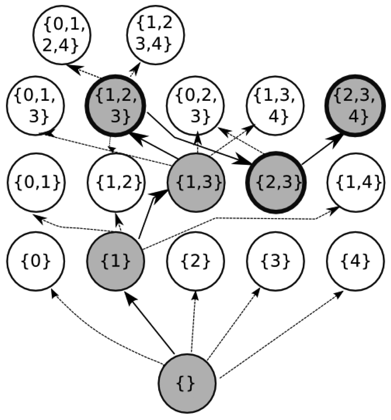
For example, suppose that there are 5 substrings that occur more than once in s and that they all have length greater than two. Let these strings be numbered from 0 to 4. We start the ZZ algorithm at the bottom node. It inspects nodes {0}, {1}, {2}, {3}, and {4}. Suppose that {1} produces the best grammar, then ZZ moves to that node and starts over exploring the nodes above it. Figure 2 shows a part of the lattice being explored. Dotted arrows point to nodes that are explored while full arrows point to nodes having the lowest score. Suppose that the algorithm then continues up until it reaches node {1, 2, 3} where no ancestor has lower score. Then ZZ starts the top-down phase, going down to node {2, 3} where no descendant has lower score. At this point a bottom-up-top-down iteration is done and the algorithm starts over again. It goes up, suppose that it reaches node {2,3,4} where it stops. Bold circled nodes correspond to nodes were the algorithm switches phases, grey nodes correspond to nodes with the best score among its siblings.
Computational Complexity
In the previous section we showed that the computational complexity of computing the score function for each node is
(n × m2), where n is the length of the target string and m is the number of substrings in the node. Every time ZZ looks for a substring to add or remove it has to inspect all possible candidates with the aim of finding the one that minimizes the score. Depending on the number of substrings that are already in the node, there might be at most
(n2) candidate strings. As a consequence, each step upwards or downwards is made in
(n2 × n × m2). Next, we need to give an upper bound for the length of the path that is potentially traversed by the algorithm. In order to define it, we first note two important properties: the score of the bottom node is equal to n and the score of any node containing more than n/2 substrings is at least n. The bottom-up phase visits at most n/2 nodes, and consequently, the top-down can only go down at most n/2 steps. Adding them together, it turns out that a bottom-up-top-down iteration traverses at most n nodes. Now, each of these iteration decreases the score by at least 1, otherwise the algorithm stops. Since the initial score is n plus the fact that the score is always positive, there can be at most n bottom-up-top-down iterations. This results in a complexity for the ZZ algorithm of
(n5 × m2).
4.3.3. Non-Monotonicity of the Search Space
We finish this section with a remark on the search space. In order to ease the understanding of the proof, we will suppose that the size of the grammar is defined as |G| = ΣA→α∈
(|α|). The proof extends easily if we consider our definition of size, but is more cumbersome (basically, instead of taking blocks of size two in the proof, take them of size three).
We have presented an algorithm that finds a local minimum on the search space. Locality is defined in terms of its direct neighborhood, but we will see that the local minimality of a node does not necessarily extend further:
Proposition 1
The lattice 〈(s), ⊆〉) is not monotonic for function score(η) = |mgp(η ∪ {s}|. That is, suppose η is a local minimum. There may be a node θ such that η ⪯ θ and score(η) > score(θ).
Proof
Consider the following sequence:
The set of possible constituents is {ab, bc, cd, de, ef, fa, da, fc, be}, none of which has size longer than 2. Note that the digrams that appear in the middle of the first blocks (of size four) appear repeated twice, while the others only once. Also, the six four-size blocks are all compositions of constituents {ab, cd, ef} (each of which is only repeated once at the end). Consider now the following grammar:
5. Experiments
In this section we experimentally compare our algorithms with the classical ones from the literature. For this purpose we use the Canterbury Corpus [23] which is a standard corpus for comparing lossless data compression algorithms. Table 1 lists the sequences of the corpus together with their length and number of repeats of length greater than one.
Not all existing algorithms are publicly available, they resolve in different ways the case when there are more than two words with the best score, they do not report results on a standard corpus or they use different definitions of the size of a grammar. In order to standardize the experiments and score, we implemented all the offline algorithms presented in this paper in the IRR framework. For the sake of completeness, we also add to the comparison LZ78 and Sequitur. Note that we have post-processed the output of the LZ78 factorizations to transform them into context-free grammars. The first series of experiments aims at comparing these classical algorithms and are shown in the middle part of Table 2. On this benchmark, we can see that IRR-MC always outputs the smallest grammars, which are on average 4.22% smaller than those of the second best (IRR-MF), confirming the partial results of [9] and showing that IRR-MC is the current state-of-the-art practical algorithm for this problem.
Then, we evaluate how the optimization of occurrences improves IRR algorithms. As shown in the IRRCOO column of Table 2, each strategy for choosing the word is improved by introducing the occurrence optimization. The sole exceptions are for the MF strategy on grammar.lsp and xargs.1, but the difference in these cases is very small and the sequences are rather short. More importantly, we can see that IRRCOO-MC is becoming the new state-of-the-art algorithm, proposing for each test a smaller grammar than IRR-MC, and being outperformed only on plrabn12.txt by IRRCOO-MF.
If given more time, these results can still be improved by using ZZ. As shown in column ZZ of Table 2, it obtains in average 3.12% smaller grammars than IRR-MC, a percentage that increases for the sequences containing natural language (for instance, for alice29.txt the gain is 8.04%), while it is lower for other sequences (only 0.1% for kennedy.xls for example). For the latter case, one can remark that the compression ratio is already very high with IRR-MC and that it may be difficult or impossible to improve it, the last few points of the percentage gain being always the hardest to achieve. As expected, ZZ improves over previous approaches mainly because it explores a much wider fraction of search space. Interestingly enough, the family of IRRCOO algorithms also improves state-of-the-art algorithms but still keeps the greedy flavour, and more importantly, it does so with a complexity cost similar to pure greedy approaches. The price to be paid for computing grammars with ZZ is its computational complexity. This problem already showed up with plrabn12.txt, lcet10.txt (where each repeat individually does not compress the sequence much, so lots of iterations are necessary) and ptt5 (which contains about 99 millions of repeats).
6. Non-Uniqueness of Smallest Grammar and Structure Discovery
Depending on the implementation, the mgp algorithm could return different small grammars using the same set of constituents because there is usually more than one shortest path in the GP-graph, and therefore there are multiple paths from which the algorithm can choose. From the point of view of data discovery, all these grammars are equally interesting if we only consider their size, but different grammars might have different structures despite having the same size.
In this section we investigate these phenomena from two different perspectives. From a theoretical point of view, we provide bounds on the number of different smallest grammars, both globally and locally (fixing the set of constituents). And from an empirical point of view, we explore and compare the actual structural variances among different grammars on some real-life sequences.
6.1. Bounds on the Number of Smallest Grammars
It is clear that a smallest grammar is not necessarily unique. Not so clear is how many smallest grammars there can be. First we will prove that for a certain family of sequences, any node of the search space corresponds to a smallest grammar. As in the proof of Proposition 1 and only to ease the understanding of the proof, we will use |G| = ΣA→α∈
(|α|) as the definition of grammar size.
Proposition 2
Let m(k) = maxs : |s|=n(number of global minima for 〈(s), ⊆〉).
Then, m(n) ∈ Ω(cn), with c > 1 constant.
Proof
It is sufficient to find one family of sequences for which the number of global minima is exponential. Consider the sequence
Now, we will suppose that the set of constituents is fixed and consider the number of smallest grammars that can be built with this set. Given a set of constituents Q we denote with
Q the set of all the smallest grammars that can be formed with Q. Different implementations of the mgp algorithm may return different grammars from
Q.
As the following Proposition shows, there are cases where the number of different smallest grammars can grow exponentially for a given set of constituents.
Proposition 3
Let .
Then m(n) ∈ Ω(cn), with c > 1 constant.
Proof
Let sk be the following sequence (aba)k and let Q be {ab, ba}. Then the mgp algorithm can parse each aba in only one of the two following ways: aA or Ba, where A and B derives ab and ba respectively. Since each occurrence of aba can be replaced by aA or Ba independently, we can see that there are 2k different ways of rewriting the body of rule sk. Moreover, all of them have the same minimal length, so there are 2k grammars of the same (minimal) size that can be formed for sk taking Q as its constituents.
Proposition 2 is complementary to Proposition 3. In the former, we prove that the number of global minima (and therefore, the number of grammars with the same minimal size) is exponential. To prove it, we provided a sequence with the property that any constituent set would yield a grammar with minimal size. In the latter we show that even if the set is fixed, still there can be an exponential number of smallest grammars with this constituent set. Not however that for the proof of Proposition 2 we needed an unbounded alphabet.
These two propositions suggest that it might not be possible to find one gold smallest grammar that could be used for structure discovery. If we consider only the size of the grammar, then all grammars in
Q are equally interesting, but different grammars might have different structures despite having the same size.
In the next section we analyze the differences among grammars of the same smallest size for a few real-life sequences. We explore their structural variances using similarity metrics and from different points of view.
6.2. An Empirical Analysis
We will now introduce a way of measuring the difference between any pair of grammars taken from
Q. Our measure is based on the fact that our grammars have a single string in their language and that string has only one derivation tree. Therefore it seems natural to use a metric that is commonly used to compare parse trees, such as Unlabeled Brackets F1 [24](also see [25] for a different explanation) in order to compare different grammars (hereafter UF1).
Summarizing the definition, the UF1 measures the overlap of the brackets sets of two parse trees. Given a grammar with a single string s in its language (which is equivalent to a parse tree) the set of brackets for that grammar is defined as the pairs of indexes in string s for which there is a non-terminal symbol that expands to that position. For instance, the initial symbol S of a grammar expands to s, so (0, |s| − 1) belongs to the bracket set of that grammar.
Full overlap of the brackets sets (UF1 = 1) implies that the two smallest grammars are equal, and the converse also holds: if two smallest grammars are equal then UF1 = 1. Also, given two smallest grammars over the same fixed constituent set, the opposite may happen. Consider again the sequence sk = (aba)k, as defined in Proposition 3, and take G1 as the grammar that rewrites every aba as aA while grammar G2 rewrites it as Ba. G1 and G2 do not share any brackets, so UF1(G1,G2) = 0.
In our experiments we will use UF1 as the way to compare structure between different smallest grammars.
Propositions 2 and 3 suggest that there are sequences for which the number of smallest grammars and the number of grammars for a given set of constituents are both exponential. Both results are based on sequences that were especially designed to show these behaviours. But it might be the case that this behaviour does not occur “naturally”. In order to shed light on this topic we present four different experiments. The first is directly focused on seeing how Proposition 3 behaves in practice and consists in computing the number of grammars with smallest size that are possible to build using the set of constituents found by the ZZ algorithm. The other three experiments analyze how different all these grammars are. Firstly, we compare the structure of different grammars randomly sampled from the set of possible grammars. Then we compare structure, as in the previous experiment, but this time, the used metric discriminates by the length of the constituents. Finally, we consider in how many different ways a single position can be parsed. The first experiment provides evidence supporting the idea of Proposition 3 being the general rule more than an exceptional case. The second group of experiments suggests that there is a common structure among all possible grammars. In particular, it suggests that longer constituents are more stable than shorter ones and that, if for each position we only consider the longest bracket that englobes it, then almost all of these brackets are common between smallest grammars.
All these experiments require a mechanism to compute different grammars sharing the same set of constituents. We provide an algorithm that not only computes this but also computes the total number of grammars that are possible to define for a given set of constituents. Let s be a sequence, and let Q be a set of constituents. An MGP-graph is a subgraph of the GP-graph used in Section 4.1 for the resolution of the MGP problem. Both have the same set of nodes but they differ in the set of edges. An edge belongs to an MGP-graph if and only if it is used in at least one of the shortest path from node 0 to node n + 1 (the end node). As a consequence, every path in an MGP-graph connecting the start node with the end one is in fact a shortest path in the GP-graph, and every path in MGP-graph defines a different way to write the rule for the initial non-terminal S. Similar subgraphs can be built for each of the non-terminal rules, and collectively we will refer to them as the MGP-graphs. Using the MGP-graphs it is possible to form a smallest grammar by simply choosing a smallest path for every MGP-graph. It only remains to explain how to compute a MGP-graph. We will do so by explaining the starting symbol case, for the rest of the non-terminals it follows in a similar fashion.
The algorithm traverses the GP-graph deleting edges and keeping those that belong to at least one shortest path. It does it in two phases. First it traverses the graph from left to right. In this phase, the algorithm assumes that the length of the smallest path from node 0 is known for every node j < i. Since all incoming edges to node i in the GP-graph come from previous nodes, it is possible to calculate the smallest path length from node 0 to node i and the algorithm only keeps those edges that are part of such paths deleting all others. The first phase produces a graph that includes paths that do not end in the final node. In order to filter out this lasts edges, the second phase of the algorithm runs a breadth-first search from the node n + 1 and goes backwards removing edges that are not involved in a smallest path.
In our experiments, we use alice29.txt, asyoulik.txt, and humdyst.chr. The first two are sequences of natural language from the Canterbury corpus, while the last one is a DNA sequence from the historical corpus of DNA used for comparing DNA compressors [26]. In all cases, the set of constituents was produced by the ZZ algorithm.
6.2.1. Counting
Using the MGP-graphs it is possible to recursively calculate the number of shortest paths that exist from the start node n0 to any other node ni. Clearly, the base case states that the number of shortest paths to n0 is equal to one. The recursive case states that the number of shortest paths to a node ni+1 is equal to the sum of the number of shortest paths of nodes nj, j ≤ i, that have an edge arriving to node ni+1.
Table 3 shows the number of different grammars that exist for our sequences. The experiments provide evidence that the number of small grammars is huge and that it might not even be tractable by a computer. These huge number of grammars pose an important question: How similar are these grammars?
6.2.2. UF1 with Random Grammars
To answer this question, we sample elements from
Q and compare them using UF1 as was described at the beginning of Section 6.2. We compare pairs of grammars, and we estimate and report average similarity between elements in
Q in Table 4.
In order to sample from
Q uniformly, we need to be able to sample each rule body, which means that we need to be able to sample complete paths (from start to end) in each MGP-graph. Using the previous algorithm for the number of smallest paths we can extend it to an algorithm that samples with uniform probability: starting at the end node, the algorithm can work its way back to the start node by repeatedly choosing one of the incoming edges with a probability proportional to the amount of smallest paths that go through that edge. The chosen edge labels form a rule body uniformly sampled among all possible ones.
6.2.3. Accounting for Constituent Sizes: UF1,k
Our second experiment aims to discover the class of brackets that make the main difference. Note that the standard UF1 measure gives the same weight to a bracket of size 2 than to longer brackets. The following experiment is quite similar to the previous one, but in order to evaluate the impact of smaller brackets in the score we introduce a new custom metric: UF1,k, which is the same that UF1 but the brackets whose length are equal or smaller than a given size k are ignored in the calculation. So when k = 1, UF1,k is equal to UF1, but for larger values of k more and more brackets are ignored in the calculation. Table 5 reports the results for different values of k. For each sequence, the table contains two columns: one for UF1,k and one for the percentage of the total brackets that were included in the calculation.
As it can be seen, the F-measure increases along k. This indicates that bigger brackets are found in most grammars of
Q, but it also shows that smaller brackets are much more numerous.
6.2.4. Conserved Parsing among Minimal Grammar Parsings
In the previous section we analyzed how different the grammars are considering different sizes of brackets. Here, we consider the differences between the grammars on single positions. The objective of this experiment is to measure the amount of different ways in which a single position of the original sequence s can be parsed by a minimal grammar. For this we will consider the partial parse tree where only the first level is retained. Doing this for each minimal grammar, we compute for each position the number of different subtrees it belongs to. This is equivalent to the number of edges that cover that position on the MGP-graph of s. If the number for one position is one for instance, this means that in all minimal grammars the same occurrence of the same non-terminal expands on this position.
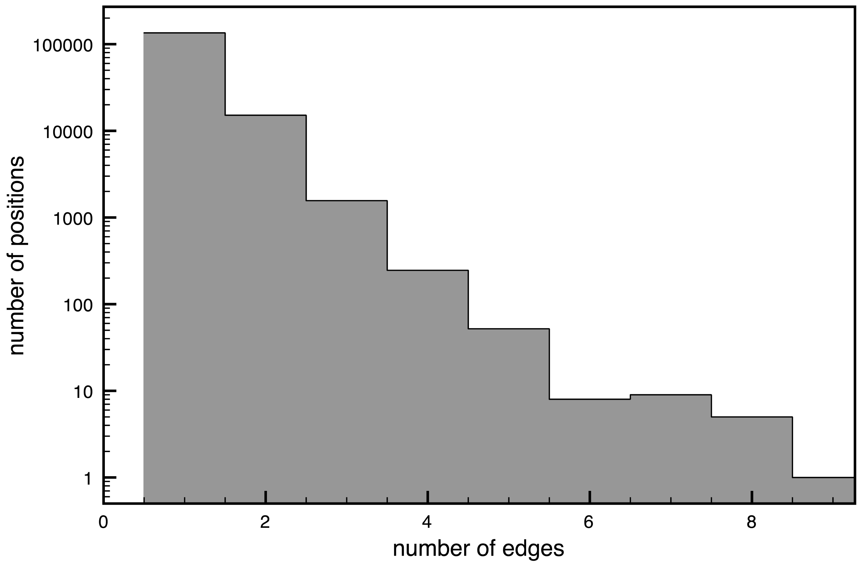
On alice29.txt, 89% of the positions are parsed exactly the same way. A histogram for all values of different parses can be seen in Figure 3. Note that the y-axis is in logarithmic scale and that the number of positions reduce drastically if the number of parses is increased: only 10% of positions are parsed in two different ways, 1% in three and all others in less than 0.2%.
There were two regions that presented peaks on the number of different symbols. Both correspond to parts in the text with long runs of the same character (white spaces): at the beginning, and in the middle during a poetry.
While this experiment is only restricted to the first level of the parse tree, it seems to indicate that the huge number of different minimal parses is due to a small number of positions where different parses have the same size. Most of the positions however are always parsed the same way.
6.3. Some Remarks
Summarising this section, we have the following theoretical results:
There can be an exponential amount of sets of constituents such that all of them produce smallest grammars (Proposition 2).
There might be two smallest grammars not sharing a single constituent other than s (from the proof of Proposition 2).
There can be an exponential amount of smallest grammars even if the set of constituents is fixed (Proposition 3).
Two smallest grammars with the same set of constituents might not share a single bracket other than the one for s (from the proof of Proposition 3).
Thus, from a theoretical point of view, there may exist structures completely incompatible between them, and nevertheless equally interesting according to the minimal size criteria. Given these results, it may be naive to expect a single, correct, hierarchical structure to emerge from approximations of a smallest grammar.
Accordingly, our experiments showed that the number of different smallest grammars grow well beyond an explicitly tractable amount.
Yet, the UF1 experiment suggested the existence of a common structure shared by the minimal grammars while the UF1,k experiment showed that this conservation involves more longer constituents than the smaller ones. The last experiment seems to indicate something similar, but concerning conservation of first-level brackets (which may not be the same as the longest brackets). One interpretation of these experiments is that, in practice, the observed number of different grammars is maybe due to the combination of all the possible parses by less significant non-terminals, while a common informative structure is conserved among the grammars. In that case, identifying the relevant structure of the sequence would require to be able to distinguish significant non-terminals, for instance by statistical tests. Meaningless constituents could also be discarded by modifying the choice function according to available background knowledge or by shifting from a pure Occam's razor point of view to a more Minimum Description Length oriented objective, which would prevent to introduce non informative non-terminals in the grammars.
7. Conclusions and Future Work
In this paper, we analyzed a new approach to the Smallest Grammar Problem, which consisted in optimizing separately the choice of words that are going to be constituents, and the choice of which occurrences of these constituents will be rewritten by non-terminals. Given a choice of constituents, we resolve the optimal choice of constituents with the polynomial-time algorithm mgp. We improve classical offline algorithms by optimizing at each step the choice of the occurrences. This permits to overcome a restriction of these classical algorithms which does not permit them to find smallest grammars.
The separation allows to define the search space as a lattice over sets of repeats where each node has an associated score corresponding to the size of the MGP of this node. We propose then a new algorithm that finds a local minimum. It explores this search space by adding, but also removing, repeats to the current set of words. Our experiments show that both approaches outperform state-of-the-art algorithms.
We then analyzed more closely how this approach can be used for structure discovery, a main application of the smallest grammar problem. While in applications of data compression and Kolmogorov complexity, we look for the size of a smallest grammar, in structure discovery the structure itself given by the grammar is the goal. We used our formalization of the smallest grammar problem to analyze the number of possible smallest grammars (globally and given a fixed set of constituents). We proved that there may be an exponential number of grammars with the same minimal size, and analyzed how different they are. Because finding the smallest grammar is intractable, we contented ourself here to study the differences between smallest grammars given the best set of constituents our algorithms were able to find. While in theory there may exist several incompatible smallest grammars, our experiments seem to confirm that, in practical cases, there is an overall stability of the different parses. We think that these results can give both some warnings and clues on how to use the result of an approximation to the smallest grammar problem for structure discovery.
The optimization of the choice of occurrences opens new perspectives when searching for the smallest grammars, especially for the inference of the structure of sequences. In future work, we want to study how this scheme actually helps to find better structure on real applications. Our efficiency concerns in this paper were oriented toward not being exponential. In future work we plan to investigate more efficient algorithms and study the compromise between execution time and final grammar size.


| Sequence | Length | # of Repeats |
|---|---|---|
| alice29.txt | 152,089 | 220,204 |
| asyoulik.txt | 125,179 | 152,695 |
| cp.html | 24,603 | 106,235 |
| fields.c | 11,150 | 56,132 |
| grammar.lsp | 3,721 | 12,780 |
| kennedy.xls | 1,029,744 | 87,427 |
| lcet10.txt | 426,754 | 853,083 |
| plrabn12.txt | 481,861 | 491,533 |
| ptt5 | 513,216 | 99,944,933 |
| sum | 38,240 | 666,934 |
| xargs.1 | 4,227 | 7,502 |
| Algorithms from the literature | Optimizing occurrences | ||||||||
|---|---|---|---|---|---|---|---|---|---|
| Sequences | Sequitur | LZ78 | IRR | IRRCOO | ZZ | ||||
| MF | ML | MC | MF | ML | MC | ||||
| alice29.txt | 49,147 | 116,296 | 42,453 | 56,056 | 41,000 | 39,794 | 52,351 | 39,251 | 37,701 |
| asyoulik.txt | 44,123 | 102,296 | 38,507 | 51,470 | 37,474 | 36,822 | 48,133 | 36,384 | 35,000 |
| cp.html | 9,835 | 22,658 | 8,479 | 9,612 | 8,048 | 8,369 | 9,313 | 7,941 | 7,767 |
| fields.c | 4,108 | 11,056 | 3,765 | 3,980 | 3,416 | 3,713 | 3,892 | 3,373 | 3,311 |
| grammar.lsp | 1,770 | 4,225 | 1,615 | 1,730 | 1,473 | 1,621 | 1,704 | 1,471 | 1,465 |
| kennedy.xls | 174,585 | 365,466 | 167,076 | 179,753 | 166,924 | 166,817 | 179,281 | 166,760 | 166,704 |
| lcet10.txt | 112,205 | 288,250 | 92,913 | 130,409 | 90,099 | 90,493 | 120,140 | 88,561 | – |
| plrabn12.txt | 142,656 | 338,762 | 125,366 | 180,203 | 124,198 | 114,959 | 164,728 | 117,326 | – |
| ptt5 | 55,692 | 106,456 | 45,639 | 56,452 | 45,135 | 44,192 | 53,738 | 43,958 | – |
| sum | 15,329 | 35,056 | 12,965 | 13,866 | 12,207 | 12,878 | 13,695 | 12,114 | 12,027 |
| xargs.1 | 2,329 | 5,309 | 2,137 | 2,254 | 2,006 | 2,142 | 2,237 | 1,989 | 1,972 |
| Sequence | humdyst.chr.seq | asyoulik.txt | alice29.txt |
|---|---|---|---|
| Sequence length | 38,770 | 125,179 | 152,089 |
| Grammar size | 10,035 | 35,000 | 37,701 |
| Number of constituents | 576 | 2391 | 2749 |
| Number of grammars | 2 × 10497 | 7 × 10968 | 8 × 10936 |
| Sequence | humdyst.chr.seq | asyoulik.txt | alice29.txt |
|---|---|---|---|
| UF1 mean | 66.02% | 81.48% | 77.81% |
| UF1 standard deviation | 1.19% | 1.32% | 1.52% |
| Smallest UF1 | 62.26% | 77.94% | 73.44% |
| Largest UF1 | 70.64% | 85.64% | 83.44% |
| k | asyoulik.txt.ij | alice29.txt.ij | humdyst.chr.seq.ij | |||
|---|---|---|---|---|---|---|
| UF1,k | Brackets | UF1,k | Brackets | UF1,k | Brackets | |
| 1 | 81.50% | 100.00% | 77.97% | 100.00% | 67.32% | 100.00% |
| 2 | 88.26% | 50.86% | 83.70% | 53.14% | 71.11% | 45.99% |
| 3 | 92.49% | 29.57% | 87.94% | 32.42% | 75.93% | 37.54% |
| 4 | 95.21% | 19.85% | 89.60% | 22.01% | 82.17% | 15.69% |
| 5 | 96.35% | 11.78% | 88.88% | 14.36% | 88.51% | 3.96% |
| 6 | 97.18% | 8.23% | 89.45% | 9.66% | 95.46% | 1.24% |
| 7 | 97.84% | 5.72% | 91.50% | 6.44% | 98.38% | 0.44% |
| 8 | 97.82% | 3.83% | 92.78% | 4.30% | 99.87% | 0.19% |
| 9 | 98.12% | 2.76% | 92.37% | 2.95% | 100.00% | 0.06% |
| 10 | 98.35% | 1.88% | 91.87% | 2.10% | 100.00% | 0.04% |
Acknowledgments
The work described in this paper was partially supported by the Program of International Scientific Cooperation MINCyT - INRIA CNRS.
References
- Charikar, M.; Lehman, E.; Liu, D.; Panigrahy, R.; Prabhakaran, M.; Sahai, A.; Shelat, A. The smallest grammar problem. IEEE Trans. Inf. Theory 2005, 51, 2554–2576. [Google Scholar]
- Rytter, W. Application of Lempel-Ziv factorization to the approximation of grammar-based compression. Theor. Comput. Sci. 2003, 302, 211–222. [Google Scholar]
- Kieffer, J.; Yang, E.H. Grammar-based codes: a new class of universal lossless source codes. IEEE Trans. Inf. Theory 2000, 46, 737–754. [Google Scholar]
- Ziv, J.; Lempel, A. Compression of Individual Sequences via Variable-Rate Coding. IEEE Trans. Inf. Theory 1978, 24, 530–536. [Google Scholar]
- Ziv, J.; Lempel, A. A Universal Algorithm for Sequential Data Compression. IEEE Trans. Inf. Theory 1977, 23, 337–343. [Google Scholar]
- Nevill-Manning, C.G. Inferring Sequential Structure. Ph.D. Thesis, University of Waikato, Hamilton, New Zealand, 1996. [Google Scholar]
- Wolff, J. An algorithm for the segmentation of an artificial language analogue. Br. J. Psychol. 1975, 66, 79–90. [Google Scholar]
- Bentley, J.; McIlroy, D. Data compression using long common strings. Proceeding of Data Compression Conference; IEEE: New York, NY, USA, 1999; pp. 287–295. [Google Scholar]
- Nevill-Manning, C.; Witten, I. On-line and off-line heuristics for inferring hierarchies of repetitions in sequences. Proceeding of Data Compression Conference; IEEE: New York, NY, USA, 2000; pp. 1745–1755. [Google Scholar]
- Apostolico, A.; Lonardi, S. Off-line compression by greedy textual substitution. Proc. IEEE 2000, 88, 1733–1744. [Google Scholar]
- Larsson, N.; Moffat, A. Off-line dictionary-based compression. Proc. IEEE 2000, 88, 1722–1732. [Google Scholar]
- Nakamura, R.; Inenaga, S.; Bannai, H.; Funamoto, T.; Takeda, M.; Shinohara, A. Linear-Time Text Compression by Longest-First Substitution. Algorithms 2009, 2, 1429–1448. [Google Scholar]
- Lanctot, J.K.; Li, M.; Yang, E.H. Estimating DNA sequence entropy. ACM-SIAM Symposium on Discrete Algorithms; Society for Industrial and Applied Mathematics: Philadelphia, PA, USA, 2000; pp. 409–418. [Google Scholar]
- Evans, S.C.; Kourtidis, A.; Markham, T.; Miller, J. MicroRNA Target Detection and Analysis for Genes Related to Breast Cancer Using MDLcompress. EURASIP J. Bioinf. Sys. Biol. 2007, 2007, 1–16. [Google Scholar]
- Nevill-Manning, C.G.; Witten, I.H. Identifying Hierarchical Structure in Sequences: A linear-time algorithm. J. Artif. Intell. Res. 1997, 7, 67–82. [Google Scholar]
- Marcken, C.D. Unsupervised language acquisition. Ph.D. Thesis, Massachusetts Institute of Technology, Cambridge, MA, USA, 1996. [Google Scholar]
- Sakakibara, Y. Efficient Learning of Context-Free Grammars from Positive Structural Examples. Inf. Comput. 1992, 97, 23–60. [Google Scholar]
- Carrascosa, R.; Coste, F.; Gallé, M.; Infante-Lopez, G. Choosing Word Occurrences for the Smallest Grammar Problem; LATA: Trier, Germany; May 24–28; 2010. [Google Scholar]
- Karpinski, M.; Rytter, W.; Shinohara, A. An efficient pattern-matching algorithm for strings with short descriptions. Nord. J. Comput. 1997, 4, 172–186. [Google Scholar]
- Gusfield, D. Algorithms on Strings, Trees, and Sequences—Computer Science and Computational Biology; Cambridge University Press: Cambridge, UK, 1997. [Google Scholar]
- Sakamoto, H.; Maruyama, S.; Kida, T.; Shimozono, S. A Space-Saving Approximation Algorithm for Grammar-Based Compression. IEICE Trans 2009, 92-D, 158–165. [Google Scholar]
- Schuegraf, E.J.; Heaps, H.S. A comparison of algorithms for data base compression by use of fragments as language elements. Inf. Storage Retr. 1974, 10, 309–319. [Google Scholar]
- Arnold, R.; Bell, T. A Corpus for the Evaluation of Lossless Compression Algorithms. Proceeding of Data Compression Conference; IEEE: Washington, DC, USA, 1997; p. 201. [Google Scholar]
- Abney, S.; Flickenger, S.; Gdaniec, C.; Grishman, C.; Harrison, P.; Hindle, D.; Ingria, R.; Jelinek, F.; Klavans, J.; Liberman, M.; Marcus, M.; Roukos, S.; Santorini, B.; Strzalkowski, T. Procedure for quantitatively comparing the syntactic coverage of English grammars. Proceedings of the Workshop on Speech and Natural Language; Black, E., Ed.; Association for Computational Linguistics: Stroudsburg, PA, USA, 1991; pp. 306–311. [Google Scholar]
- Klein, D. The Unsupervised Learning of Natural Language Structure. Ph.D. Thesis, University of Stanford, Stanford, CA, USA, 2005. [Google Scholar]
- Manzini, G.; Rastero, M. A simple and fast DNA compressor. Softw. Pract. Exp. 2004, 34, 1397–1411. [Google Scholar]
© 2011 by the authors; licensee MDPI, Basel, Switzerland. This article is an open access article distributed under the terms and conditions of the Creative Commons Attribution license (http://creativecommons.org/licenses/by/3.0/).
Share and Cite
Carrascosa, R.; Coste, F.; Gallé, M.; Infante-Lopez, G. The Smallest Grammar Problem as Constituents Choice and Minimal Grammar Parsing. Algorithms 2011, 4, 262-284. https://doi.org/10.3390/a4040262
Carrascosa R, Coste F, Gallé M, Infante-Lopez G. The Smallest Grammar Problem as Constituents Choice and Minimal Grammar Parsing. Algorithms. 2011; 4(4):262-284. https://doi.org/10.3390/a4040262
Chicago/Turabian StyleCarrascosa, Rafael, François Coste, Matthias Gallé, and Gabriel Infante-Lopez. 2011. "The Smallest Grammar Problem as Constituents Choice and Minimal Grammar Parsing" Algorithms 4, no. 4: 262-284. https://doi.org/10.3390/a4040262