A Finite Element Flux-Corrected Transport Method for Wave Propagation in Heterogeneous Solids

Abstract

When moving discontinuities in solids need to be simulated, standard finite element (FE) procedures usually attain low accuracy because of spurious oscillations appearing behind the discontinuity fronts. To assure an accurate tracking of traveling stress waves in heterogeneous media, we propose here a flux-corrected transport (FCT) technique for structured as well as unstructured space discretizations. The FCT technique consists of post-processing the FE velocity field via diffusive/antidiffusive fluxes, which rely upon an algorithmic length-scale parameter. To study the behavior of heterogeneous bodies featuring compliant interphases of any shape, a general scheme for computing diffusive/antidiffusive fluxes close to phase boundaries is proposed too. The performance of the new FE-FCT method is assessed through one-dimensional and two-dimensional simulations of dilatational stress waves propagating along homogeneous and composite rods.

1. Introduction

The propagation of waves in elastic solids is governed by a second-order, hyperbolic differential equation. Waves therefore travel inside bodies with a finite speed, and cause an abrupt change of the local velocity and stress fields across their fronts.

Numerical methods have to accurately track such moving inner discontinuities. Since standard dis-placement-based finite element (FE) schemes adopt continuous interpolation fields to mimic the discontinuous ones inside the modeled domain, non-physical high-frequency oscillations show up around wave fronts; these oscillations are a numerical artifact and need to be filtered out of the solution. Algorithmic treatments of this issue have been proposed in the literature, and they typically consist in artificial viscosity or mesh adaption. Focusing on time integration, algorithms like the $\alpha$-method [1] or the generalized $\alpha$-method [2] were also devised to damp oscillations. All these methods can reduce in size such spurious effects, but sometimes entail energy dissipation which is, again, non-physical.

An alternative treatment, whose roots can be traced back to the seminal work of Boris & Book [3,4], is the flux-corrected transport (FCT) method. The FCT algorithm consists of post-processing a standard FE solution: diffusive and antidiffusive fluxes, the latter being appropriately limited in size, are handled to improve the discrete velocity field around the discontinuities, and to filter out spurious oscillations. This method has been extensively used to simulate the propagation of shock waves in fluids [5,6]; recently, it has been adopted to simulate traveling stress waves in solids [7]. Noteworthy results have been obtained in [8] through a coupling of a displacement-based FE solution and the FCT algorithm; owing to the adopted structured meshes, results for bodies of arbitrary shapes were based on a partition-of-unity enrichment of the nodal shape functions.

In this work, to study the dynamics of heterogeneous bodies we propose two enhancements to the frame developed in [8,9]. First, to simulate the propagation of stress waves inside domains of arbitrary shape, an algorithmic length-scale ${\ell }_{\text{FCT}}$ is introduced: this length-scale allows to define local supports of finite size, which are independent of the space discretization, wherein diffusive/antidiffusive fluxes are computed. Second, the rationale behind the computation of diffusive/antidiffusive fluxes close to body or phase boundaries is revisited, so as to permit the treatment of compliant interphases confined along loci of zero measure (i.e. surfaces in three-dimensional frames and lines in two-dimensional frames).

These two enhancements are of paramount importance when dynamic failure of quasi-brittle polycrystals (like, e.g., polysilicon) needs to be modeled, since damaging phenomena at the micro-scale are incepted as soon as the tensile strength is locally attained. Because of the polycrystal micro-structure, traveling waves are partially reflected by each grain boundary, and eventually lead to complex stress patterns. If the numerical solution does contain the aforementioned fictitious oscillations, the amplitude of the local stress field may be artificially increased and, therefore, damage wrongly started. Through simulations of stress waves traveling along homogeneous as well as heterogeneous (bimaterial) rods, we show that the proposed FE-FCT method can be used to accurately study the evolution of the stress field in quasi-brittle polycrystals.

As far as notation is concerned, a matrix one will be adopted throughout the whole paper with uppercase and lowercase bold symbols respectively denoting matrices and vectors, a superscript ${}^{\text{T}}$ standing for transpose, and a superposed dot representing time rates.

2. Dynamics of heterogeneous bodies

2.1. Governing relations

Let Ω be a heterogeneous three-dimensional body; its smooth outer boundary, with unit outward normal $\mathbf{m}$, be constituted by the two disjoint sets ${\Gamma }_u$ and ${\Gamma }_{\tau }$, where displacements and tractions are respectively assigned. Without any loss of generality, let us assume that Ω is a continuum made of two phases (${\Omega }^{+}$ and ${\Omega }^{-}$, with $\Omega ={\Omega }^{+}\cup {\Omega }^{-}$), tied together in the initial configuration along the flat interface Γ, see Figure 1. Γ actually represents the interphase between ${\Omega }^{+}$ and ${\Omega }^{-}$; since the thickness of this interphase is usually at least one order of magnitude smaller than the characteristic size of Ω, the interphase itself is modeled as a zero-thickness interface. Damaging processes along Γ may cause opening (mode I) and/or sliding (mode II and mode III) displacement discontinuities in the $\mathbf{n}$ direction and in the ${\mathbf{s}}_1-{\mathbf{s}}_2$ plane, respectively.

Figure 1. Geometry of a two-phase body, and notation.

Figure 1. Geometry of a two-phase body, and notation.

The equilibrium of Ω at time t is governed by:

$$\begin{array}{cccc}\hfill {\mathcal{C}}^{\text{T}}\sigma +\overline{\mathbf{b}}=& \varrho \ddot{\mathbf{u}}\hfill & \hfill & \text{in}\Omega \setminus \Gamma \hfill \end{array}$$

(1)

$$\begin{array}{cccc}\hfill \mathcal{M}\sigma =& \overline{\tau }\hfill & \hfill & \text{on}{\Gamma }_{\tau }\hfill \end{array}$$

(2)

$$\begin{array}{cccc}\hfill \mathcal{N}\sigma =& -\tau \hfill & \hfill & \text{on}{\Gamma }^{+}\hfill \end{array}$$

(3)

$$\begin{array}{cccc}\hfill \mathcal{N}\sigma =& \tau \hfill & \hfill & \text{on}{\Gamma }^{-}\hfill \end{array}$$

(4)

where ${\Gamma }^{+}$ and ${\Gamma }^{-}$ are the sides of Γ respectively belonging to ${\Omega }^{+}$ and ${\Omega }^{-}$, and according to Voigt’s notation [10]: σ is the stress vector, which gathers the independent components of the stress tensor; $\overline{\mathbf{b}}$ and $\overline{\tau }$ are the assigned loads in the bulk $\Omega \setminus \Gamma$ and along ${\Gamma }_{\tau }$; ϱ is the mass density of the bulk material; $\ddot{\mathbf{u}}$ is the acceleration in $\Omega \setminus \Gamma$; $\mathcal{C}$ is the differential compatibility operator; $\mathcal{M}$ and $\mathcal{N}$ are the matrices collecting the components of the unit vectors $\mathbf{m}$ and $\mathbf{n}$.

In the small strain regime, compatibility reads:

$$\begin{array}{cccc}\hfill \epsilon =& \mathcal{C}\mathbf{u}\hfill & \hfill & \text{in}\Omega \setminus \Gamma \hfill \end{array}$$

(5)

$$\begin{array}{cccc}\hfill \mathbf{u}]=& \mathbf{u}{|}_{{\Gamma }^{+}}-\mathbf{u}{|}_{{\Gamma }^{-}}\hfill & \hfill & \text{on}\Gamma \hfill \end{array}$$

(6)

$$\begin{array}{cccc}\hfill \mathbf{u}=& \overline{\mathbf{u}}\hfill & \hfill & \text{on}{\Gamma }_u\hfill \end{array}$$

(7)

where: ε is the strain vector; $\mathbf{u}$ is the displacement in Ω; $\left[\mathbf{u}\right]$ is the displacement discontinuity along Γ; $\overline{\mathbf{u}}$ is the assigned displacement along ${\Gamma }_u$.

The body is conceived to be initially at rest, i.e.:

$${\mathbf{u}}_0=\mathbf{0},{\dot{\mathbf{u}}}_0=\mathbf{0}\text{in}\Omega$$

(8)

As far as constitutive modeling is concerned, the bulk is assumed to behave elastically according to:

$$\begin{array}{c}\hfill \sigma ={\mathbf{E}}_{\Omega }\epsilon \text{in}\Omega \setminus \Gamma \end{array}$$

(9)

where ${\mathbf{E}}_{\Omega }$ is the bulk elasticity matrix. Along Γ, damage can be incepted once a local strength criterion is satisfied; to simplify matters we assume that the stress waves do not cause any dissipative phenomena. The interface thus behaves elastically too, according to:

$$\begin{array}{c}\hfill \tau ={\mathbf{E}}_{\Gamma }\left[\mathbf{u}\right]\text{on}\Gamma \end{array}$$

(10)

${\mathbf{E}}_{\Gamma }$ being the interface elasticity matrix.

2.2. Space-time discretized solution

The weak form of the equilibrium equations (1)-(4), allowing for bulk and interface constitutive laws (9)-(10), reads [11,12,13]:

$$\begin{array}{cc}\hfill \text{find}\mathbf{u}\in \mathcal{U}:\underset{\Omega \setminus \Gamma }{\int }\varrho {\mathbf{v}}^{\text{T}}\ddot{\mathbf{u}}d\Omega +\underset{\Omega \setminus \Gamma }{\int }{\epsilon }_v^{\text{T}}{\mathbf{E}}_{\Omega }\epsilon d\Omega +& \underset{\Gamma }{\int }{\left[\mathbf{v}\right]}^{\text{T}}{\mathbf{E}}_{\Gamma }\left[\mathbf{u}\right]d\Gamma \hfill \\ \hfill =& \underset{\Omega \setminus \Gamma }{\int }{\mathbf{v}}^{\text{T}}\overline{\mathbf{b}}d\Omega +\underset{{\Gamma }_{\tau }}{\int }{\mathbf{v}}^{\text{T}}\overline{\tau }d{\Gamma }_{\tau }\forall \mathbf{v}\in {\mathcal{U}}_0\hfill \end{array}$$

(11)

where: $\mathbf{v}$ is the test function, and ${\epsilon }_v=\mathcal{C}\mathbf{v}$; $\mathcal{U}$ is the trial solution space, featuring displacement fields $\mathbf{u}$ continuous in $\Omega \setminus \Gamma$, possibly discontinuous along Γ, and fulfilling the boundary condition (7) on ${\Gamma }_u$; ${\mathcal{U}}_0$ is the relevant variation space. In view of the assumed linearized kinematics, $\Gamma \equiv {\Gamma }^{+}\equiv {\Gamma }^{-}$ holds for the interface.

Now, let the finite element approximation of the displacement, displacement jump and deformation fields be:

$$\begin{array}{cc}\hfill \mathbf{u}\cong & \Phi {\mathbf{u}}^h\hfill \end{array}$$

(12)

$$\begin{array}{cc}\hfill \mathbf{u}]\cong & {\mathbf{B}}_{\Gamma }{\mathbf{u}}^h\hfill \end{array}$$

(13)

$$\begin{array}{cc}\hfill \epsilon \cong & \mathcal{C}\Phi {\mathbf{u}}^h={\mathbf{B}}_{\Omega }{\mathbf{u}}^h\hfill \end{array}$$

(14)

where: ${\mathbf{u}}^h$ is the nodal displacement vector; Φ is the matrix of nodal shape functions; ${\mathbf{B}}_{\Gamma }$ and ${\mathbf{B}}_{\Omega }$ are, respectively, the interface and bulk compatibility matrices. The semi-discretized equations of motion of the solid turn out to be:

$$\mathbf{M}{\ddot{\mathbf{u}}}^h+\left({\mathbf{K}}_{\Omega }+{\mathbf{K}}_{\Gamma }\right){\mathbf{u}}^h=\mathbf{F}$$

(15)

where the mass matrix $\mathbf{M}$, the bulk and interface stiffness matrices ${\mathbf{K}}_{\Omega }$ and ${\mathbf{K}}_{\Gamma }$, and the external load vector $\mathbf{F}$ are:

$$\begin{array}{cc}\hfill \mathbf{M}=& \underset{\Omega \setminus \Gamma }{\int }\varrho {\Phi }^{\text{T}}\Phi d\Omega \hfill \end{array}$$

(16)

$$\begin{array}{cc}\hfill {\mathbf{K}}_{\Omega }=& \underset{\Omega \setminus \Gamma }{\int }{\mathbf{B}}_{\Omega }^{\text{T}}{\mathbf{E}}_{\Omega }{\mathbf{B}}_{\Omega }d\Omega \hfill \end{array}$$

(17)

$$\begin{array}{cc}\hfill {\mathbf{K}}_{\Gamma }=& \underset{\Gamma }{\int }{\mathbf{B}}_{\Gamma }^{\text{T}}{\mathbf{E}}_{\Gamma }{\mathbf{B}}_{\Gamma }d\Gamma \hfill \end{array}$$

(18)

$$\begin{array}{cc}\hfill \mathbf{F}=& \underset{\Omega \setminus \Gamma }{\int }{\Phi }^{\text{T}}\overline{\mathbf{b}}d\Omega +\underset{{\Gamma }_{\tau }}{\int }{\Phi }^{\text{T}}\overline{\tau }d{\Gamma }_{\tau }\hfill \end{array}$$

(19)

To advance the solution of (15) in time we employ an explicit Newmark method. Having partitioned the time interval of interest according to $\left[t_0{t}_N\right]={\cup }_{i=0}^{N_t-1}\left[t_i{t}_{i+1}\right]$, within the time step $\left[t_i{t}_{i+1}\right]$ a predictor-integrator-corrector splitting is followed according to:

• predictor:

  $$\begin{array}{cc}\hfill {\tilde{\mathbf{u}}}_{i+1}=& {\mathbf{u}}_i+\Delta t{\dot{\mathbf{u}}}_i+\Delta t^2\left({\displaystyle \frac{1}{2}}-\beta \right){\ddot{\mathbf{u}}}_i\hfill \end{array}$$

  (20)

  $$\begin{array}{cc}\hfill {\dot{\tilde{\mathbf{u}}}}_{i+1}=& {\dot{\mathbf{u}}}_i+\Delta t(1-\gamma ){\ddot{\mathbf{u}}}_i\hfill \end{array}$$

  (21)

  where $\Delta t=t_{i+1}-t_i$;
• explicit integrator:

  $${\ddot{\mathbf{u}}}_{i+1}={\mathbf{M}}^{-1}\left({\mathbf{F}}_{i+1}-\left({\mathbf{K}}_{\Omega }+{\mathbf{K}}_{\Gamma }\right){\tilde{\mathbf{u}}}_{i+1}\right)$$

  (22)
• corrector:

  $$\begin{array}{cc}\hfill {\mathbf{u}}_{i+1}=& {\tilde{\mathbf{u}}}_{i+1}+\Delta t^2\beta {\ddot{\mathbf{u}}}_{i+1}\hfill \end{array}$$

  (23)

  $$\begin{array}{cc}\hfill {\dot{\overline{\mathbf{u}}}}_{i+1}=& {\dot{\tilde{\mathbf{u}}}}_{i+1}+\Delta t\gamma {\ddot{\mathbf{u}}}_{i+1}\hfill \end{array}$$

  (24)

To resemble the average acceleration scheme, which is unconditionally stable and second-order accurate, $\beta =0.25$ and $\gamma =0.5$ are adopted in the preceding equations.

The time step size $\Delta t$ has been always set so as to fulfill the Courant condition in the bulk $\Omega \setminus \Gamma$. Moreover, to speed up the explicit integrator phase (22), the mass matrix $\mathbf{M}$ has been diagonalized via row-sum lumping [14].

Customary FE methods finally assume ${\dot{\mathbf{u}}}_{i+1}={\dot{\overline{\mathbf{u}}}}_{i+1}$, without any treatment to avoid the occurrence of spurious oscillations. With the FCT scheme, instead, a post-processing stage is added to deal with such an issue; details on this phase are furnished in Section 3

3. Flux-corrected transport method

We already pointed out that the accuracy of customary FE simulations of moving discontinuities, as obtained via the procedure outlined in Section 2.2, is usually spoiled by oscillations first arising around the discontinuity fronts, where both the velocity and stress fields are discontinuous.

Figure 2. Deployment of points for the computation of FCT diffusive/antidiffusive fluxes: (a) structured mesh case; (b) unstructured mesh case.

Figure 2. Deployment of points for the computation of FCT diffusive/antidiffusive fluxes: (a) structured mesh case; (b) unstructured mesh case.

To avoid such kind of fictitious oscillations, the FCT algorithm has been adopted in [8,15,16]: it amounts to post-processing the local velocity field, which actually suffers discontinuities, via viscous-like diffusive and antidiffusive fluxes, the latter ones being appropriately limited in size. For ease of notation, we detail here the algorithm in the case of a one-dimensional domain Ω; pointing to the $j-$th node of the space discretization and assuming the mesh to be structured, the standard version of the FCT algorithm reads:

• compute diffusive fluxes:

  $$\begin{array}{cc}\hfill {\phi }_D^{j-1/2}=& {\eta }_D({\dot{u}}_i^j-{\dot{u}}_i^{j-1})\hfill \end{array}$$

  (25)

  $$\begin{array}{cc}\hfill {\phi }_D^{j+1/2}=& {\eta }_D({\dot{u}}_i^{j+1}-{\dot{u}}_i^j)\hfill \end{array}$$

  (26)
• update the solution through diffusive fluxes:

  $$\begin{array}{c}\hfill {\dot{\widehat{u}}}_{i+1}^j={\dot{\overline{u}}}_{i+1}^j+{\phi }_D^{j+1/2}-{\phi }_D^{j-1/2}\end{array}$$

  (27)
• compute anti-diffusive fluxes:

  $$\begin{array}{cc}\hfill {\phi }_A^{j-1/2}=& {\eta }_A({\dot{\overline{u}}}_i^j-{\dot{\overline{u}}}_i^{j-1})\hfill \end{array}$$

  (28)

  $$\begin{array}{cc}\hfill {\phi }_A^{j+1/2}=& {\eta }_A({\dot{\overline{u}}}_i^{j+1}-{\dot{\overline{u}}}_i^j)\hfill \end{array}$$

  (29)
• apply limitation to antidiffusive fluxes:

  $$\begin{array}{cc}\hfill {\overline{\phi }}_A^{j-1/2}=& S^{j-1/2}max\left\{0,min\left\{S^{j-1/2}\left({\dot{\widehat{u}}}_{i+1}^{j-1}-{\dot{\widehat{u}}}_{i+1}^{j-2}\right),\left|{\phi }_A^{j-1/2}\right|,S^{j-1/2}\left({\dot{\widehat{u}}}_{i+1}^{j+1}-{\dot{\widehat{u}}}_{i+1}^j\right)\right\}\right\}\hfill \end{array}$$

  (30)

  $$\begin{array}{cc}\hfill {\overline{\phi }}_A^{j+1/2}=& S^{j+1/2}max\left\{0,min\left\{S^{j+1/2}\left({\dot{\widehat{u}}}_{i+1}^j-{\dot{\widehat{u}}}_{i+1}^{j-1}\right),\left|{\phi }_A^{j+1/2}\right|,S^{j+1/2}\left({\dot{\widehat{u}}}_{i+1}^{j+2}-{\dot{\widehat{u}}}_{i+1}^{j+1}\right)\right\}\right\}\hfill \end{array}$$

  (31)

  where $S^{j-1/2}=\text{sign}\left({\phi }_A^{j-1/2}\right)$ and $S^{j+1/2}=\text{sign}\left({\phi }_A^{j+1/2}\right)$

Figure 3. Sketch of the shape of nodal supports, either when they are wholly included in Ω or when they intersect the boundary of any phase.

Figure 3. Sketch of the shape of nodal supports, either when they are wholly included in Ω or when they intersect the boundary of any phase.

• update the solution through limited antidiffusive fluxes:

  $$\begin{array}{c}\hfill {\dot{u}}_{i+1}^j={\dot{\widehat{u}}}_{i+1}^j-{\overline{\phi }}_A^{j+1/2}+{\overline{\phi }}_A^{j-1/2}\end{array}$$

  (32)
• enforce boundary conditions.

In the above equations: terms ${\dot{u}}^{j-1}$ and ${\dot{u}}^{j+1}$ respectively denote the velocities at the nodes on the left and right sides of the $j-$th one, see Figure 2(a); ${\eta }_D$ and ${\eta }_A$ are the diffusive and antidiffusive coefficients. In two- and three-dimensional settings the above procedure can be generalized by following the same path to correct the velocity component aligned with each reference axis.

As far as the computational burden of the proposed FE-FCT scheme is concerned, it can said that: the explicit Newmark time integration consists of the five loops (20)-(24) over the nodes; the FCT algorithm consists of the eight loops (25)-(32) over the nodes, and of some additional operations in (30)-(31) (i.e. min, max, positive part). Hence, in terms of computing time, simulations run with the present FE-FCT scheme turn out to be at least $\frac{13}{5}=2.6$ times longer than the corresponding customary FE ones.

When discontinuities travel inside irregular domains, ad-hoc procedures have been followed to fulfill boundary conditions or to model the response of multi-phase materials, see e.g. [8]. In this work we offer a simple procedure to allow also the adoption of unstructured meshes: in the above equations, instead of using nodal information to update the velocity field, we handle information on a local grid centered at the $j$-th node and characterized by a constant spacing among grid points, see Figure 2(b). This spacing between grid points, termed ${\ell }_{\text{FCT}}$, is not to be meant as the distance between neighboring nodes, but instead an algorithmic parameter to be tuned. The velocity at each point of this grid is obtained from the nodal ones through interpolation, using the shape functions gathered in Φ (see Equation 12).

A proof of the conservation of local momenta, or error estimators for the conservation laws are beyond the goals of this paper, and are left for future investigations.

Figure 4. Longitudinal wave propagation in a two-phase rod: sketch of geometry and loading condition.

Figure 4. Longitudinal wave propagation in a two-phase rod: sketch of geometry and loading condition.

Figure 5. Wave propagating along a homogeneous rod discretized with a structured mesh: stress field at (a) $t=0.5·{10}^{-2}$ s and at (b) $t=1.8·{10}^{-2}$ s. Blue solid line: FE solution; black solid line: standard FE-FCT solution; orange dashed line: newly proposed FE-FCT solution.

Figure 5. Wave propagating along a homogeneous rod discretized with a structured mesh: stress field at (a) $t=0.5·{10}^{-2}$ s and at (b) $t=1.8·{10}^{-2}$ s. Blue solid line: FE solution; black solid line: standard FE-FCT solution; orange dashed line: newly proposed FE-FCT solution.

To deal with compliant interfaces, whose behavior is described by constitutive laws like Equation (5), a specific treatment of phase boundaries is needed. Here we propose the following rationale: during the FCT correction step, each phase is assumed to be an independent body. Therefore, if a local support intersects either the outer boundary ${\Gamma }_u\cup {\Gamma }_{\tau }$ or the interface Γ, it is re-shaped according to what sketched in Figure 3. Since in Equations (25)-(32) the $(j-2)$-th, $(j-1)$-th, $(j+1)$-th and $(j+2)$-th terms are dropped when the relevant points (or nodes in the standard formulation) fall outside Ω, the algorithm is enhanced by adopting the same criterion if grid points fall outside the phase the $j$-th node belongs to. If this procedure is not followed, the FCT correction step can not feel interfaces endowed with their own constitutive laws.

Forthcoming results will show that the two enhancements here proposed permit to increase much the accuracy of FE results, specially close to stress wave fronts, by preventing macroscopic fluctuations to show up in the velocity and stress fields, even when unstructured space discretizations are adopted.

Figure 6. Wave propagating along a homogeneous rod discretized with an unstructured mesh: stress field at $t=1.8·{10}^{-2}$ s. Blue solid line: FE solution; black solid line: standard FE-FCT solution; orange dashed line: newly proposed FE-FCT solution.

Figure 6. Wave propagating along a homogeneous rod discretized with an unstructured mesh: stress field at $t=1.8·{10}^{-2}$ s. Blue solid line: FE solution; black solid line: standard FE-FCT solution; orange dashed line: newly proposed FE-FCT solution.

4. Longitudinal waves in homogeneous and heterogeneous rods

To assess the capability of the newly proposed FE-FCT method, the propagation of (longitudinal) waves in homogeneous as well as heterogeneous slender bodies (rods) is simulated. To check the accuracy of the method, results are compared to an analytical solution derived next.

4.1. Analytical solution

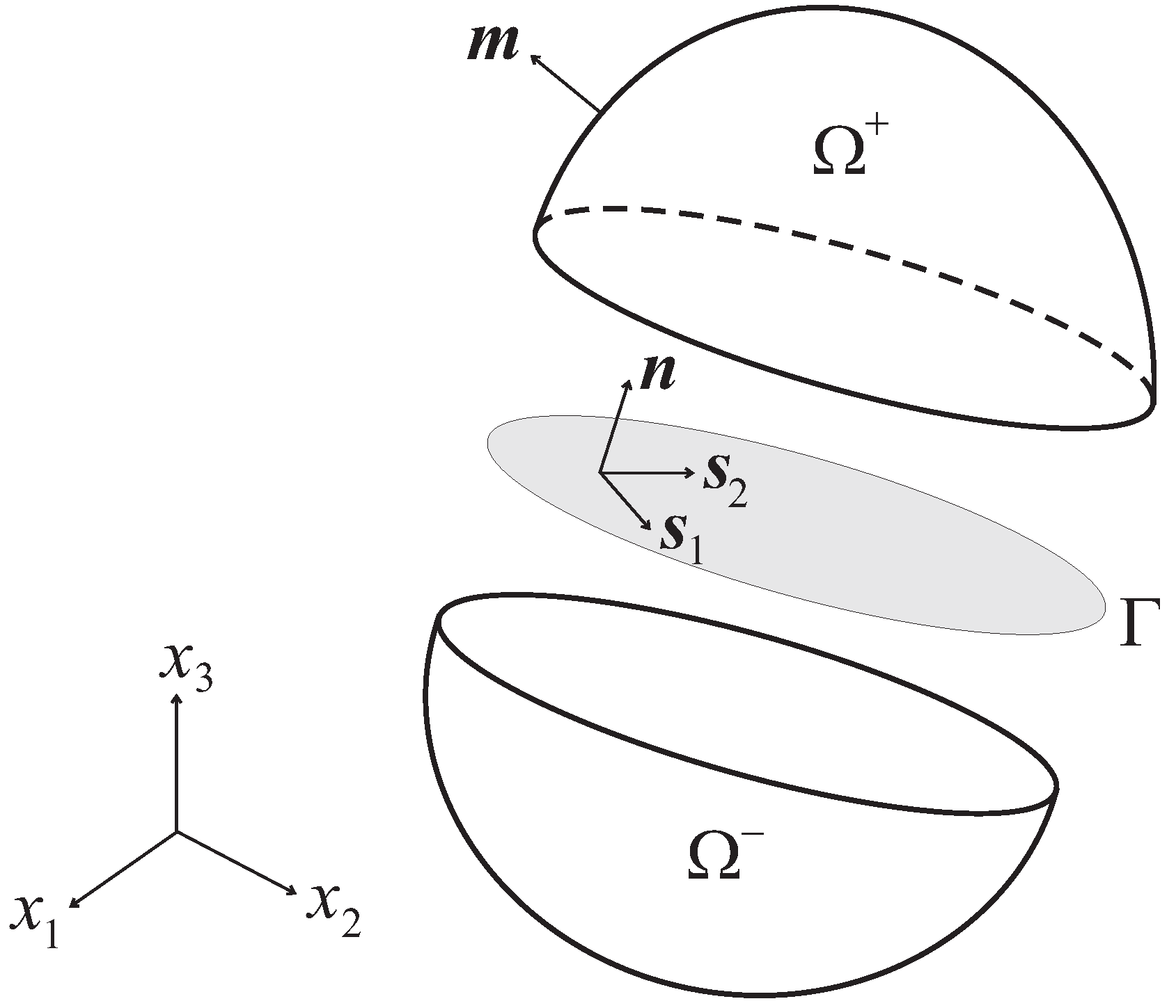
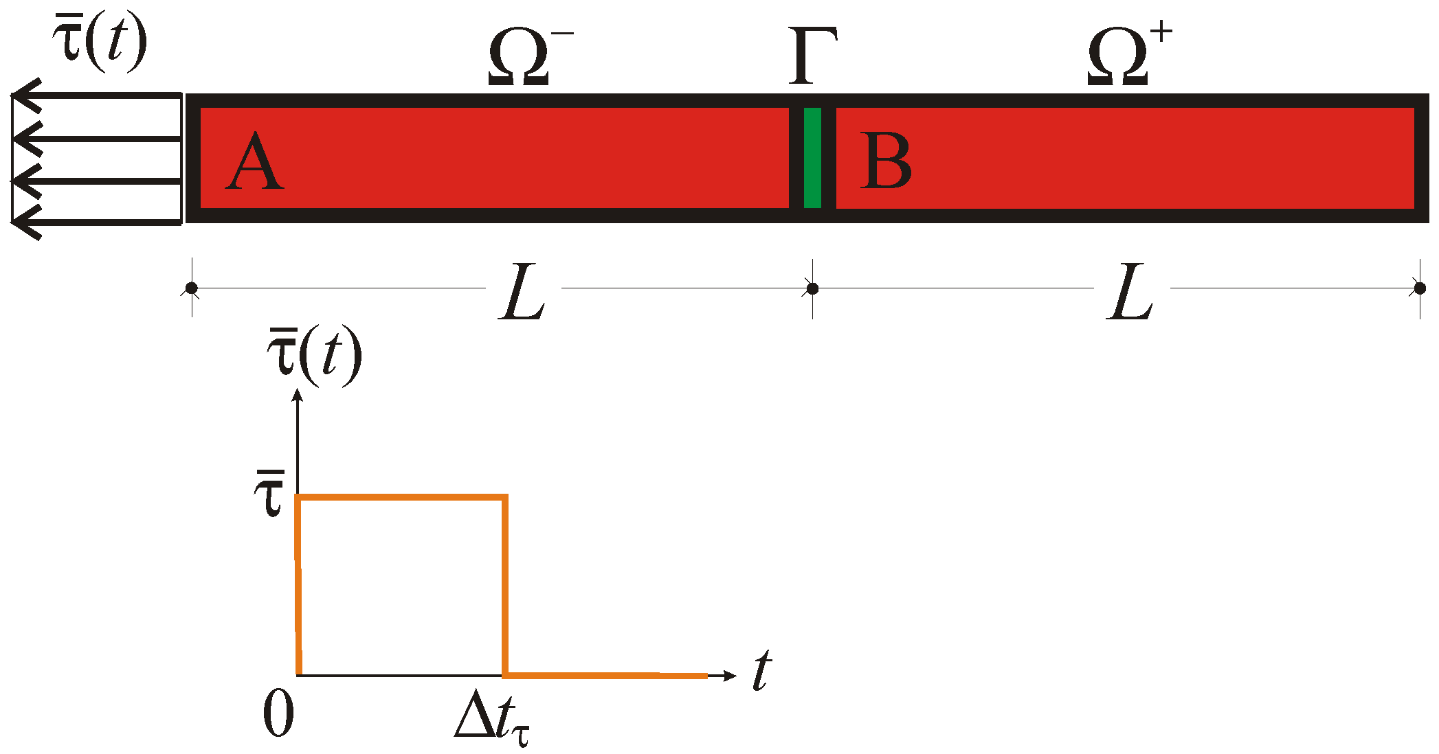
Let Ω be a slender body, such that only the propagation of longitudinal waves is of interest. According to the schematic of Figure 4, the body is assumed to be loaded by a constant pressure $\overline{\tau }$, acting over the time interval $\Delta t_{\tau }$. To get insights into the effect of inner boundaries on wave reflection and dispersion, a two-phase body in considered, with phases A and B (of length L in the direction of wave propagation) respectively featuring Young’s moduli $E_A$ and $E_B$, and mass densities ${\varrho }_A$ and ${\varrho }_B$; the relevant longitudinal wave speeds thus are $c_A=\sqrt{\frac{E_A}{{\varrho }_A}}$ and $c_B=\sqrt{\frac{E_B}{{\varrho }_B}}$.

In view of the elastic response of the bulk, a tensile wave propagating inside material A turns out to be characterized by the following relationship between the stress amplitude ${\sigma }_{\text{in}}$ and the particle velocity $v_{\text{in}}$:

$${\sigma }_{\text{in}}=-{\varrho }_A{c}_A{v}_{\text{in}}$$

(33)

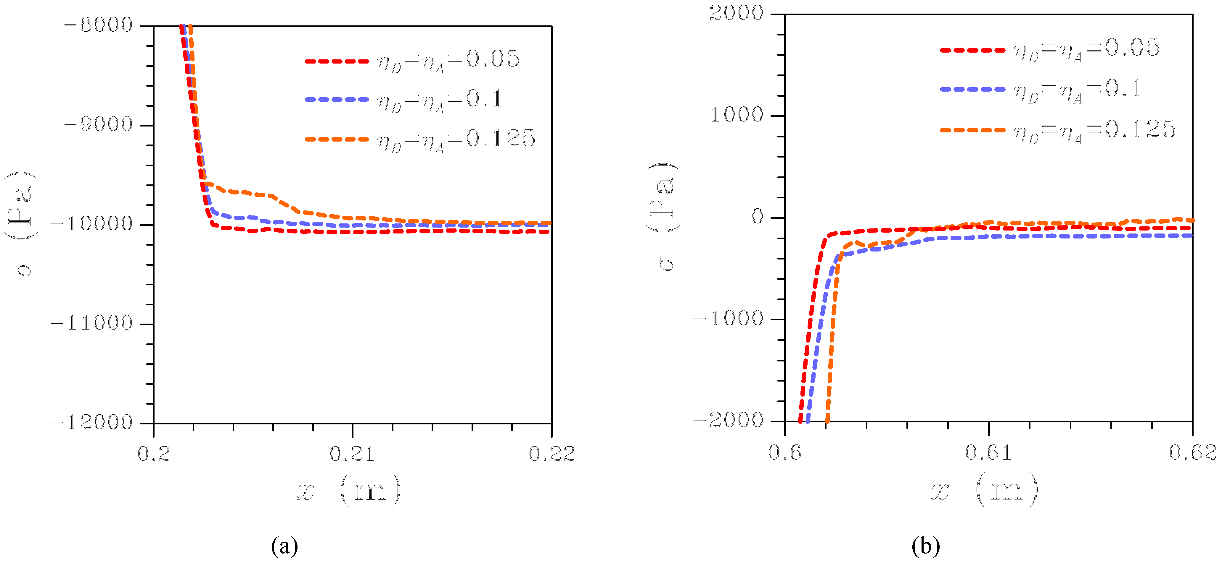
Figure 7. Wave propagating along a homogeneous rod discretized with an unstructured mesh: stress field at $t=1.8·{10}^{-2}$ s. Effect of parameters ${\eta }_D={\eta }_A$ on the capability of the newly proposed FE-FCT scheme to accurately track the stress discontinuity across the wave fronts.

Figure 7. Wave propagating along a homogeneous rod discretized with an unstructured mesh: stress field at $t=1.8·{10}^{-2}$ s. Effect of parameters ${\eta }_D={\eta }_A$ on the capability of the newly proposed FE-FCT scheme to accurately track the stress discontinuity across the wave fronts.

After impinging upon the interface Γ at $t=\overline{t}$, the incident wave induces reflected and transmitted waves, respectively characterized by relations [17]:

$$\begin{array}{cc}\hfill {\sigma }^{-}=& +{\varrho }_A{c}_A{v}^{-}\hfill \end{array}$$

(34)

$$\begin{array}{cc}\hfill {\sigma }^{+}=& -{\varrho }_B{c}_B{v}^{+}\hfill \end{array}$$

(35)

where ${\sigma }^{-}$ and ${\sigma }^{+}$ are the amplitudes of the reflected and transmitted stress waves, and $v^{-}$ and $v^{+}$ are the relevant particle velocities. Equilibrium across Γ requires:

$$\begin{array}{c}\hfill {\sigma }_{\text{in}}+{\sigma }^{-}={\sigma }^{+}\end{array}$$

(36)

while compatibility reads:

$$\begin{array}{c}\hfill \left[\dot{u}\right]=v^{+}-\left(v_{\text{in}}+v^{-}\right)\end{array}$$

(37)

$\left[\dot{u}\right]$ being the opening velocity on Γ. Account taken of the interface constitutive law (10), written for mode I loadings as $\tau \equiv {\sigma }^{+}=E_{\Gamma }\left[u\right]$, one arrives at the differential equation:

$$\begin{array}{c}\hfill {\dot{\sigma }}^{+}={\displaystyle \frac{1}{t_c}}\left({\sigma }_{\text{in}}-{\displaystyle \frac{\gamma +1}{2\gamma }}{\sigma }^{+}\right)\end{array}$$

(38)

where: $t_c=\frac{{\varrho }_A{c}_A}{2E_{\Gamma }}$ is the time-scale of the opening process along interface Γ (sometimes called characteristic relaxation time [17]); $\gamma =\frac{{\varrho }_B{c}_B}{{\varrho }_A{c}_A}$. Upon integration of (38), the solution in terms of time histories of the reflected and transmitted waves reads:

$$\begin{array}{cc}\hfill {\sigma }^{-}=& \left({\displaystyle \frac{\gamma -1}{2\gamma }}-exp\left[-\frac{\gamma +1}{2\gamma }\frac{t-\overline{t}}{t_c}\right]\right){\displaystyle \frac{2\gamma }{\gamma +1}}{\sigma }_{\text{in}}\hfill \end{array}$$

(39)

$$\begin{array}{cc}\hfill {\sigma }^{+}=& \left(1-exp\left[-\frac{\gamma +1}{2\gamma }\frac{t-\overline{t}}{t_c}\right]\right){\displaystyle \frac{2\gamma }{\gamma +1}}{\sigma }_{\text{in}}\hfill \end{array}$$

(40)

Figure 8. Wave propagating along a homogeneous rod discretized with a two-dimensional unstructured mesh: longitudinal stress field at (top) $t=0.5·{10}^{-2}$ s and (bottom) $t=1.8·{10}^{-2}$ s.

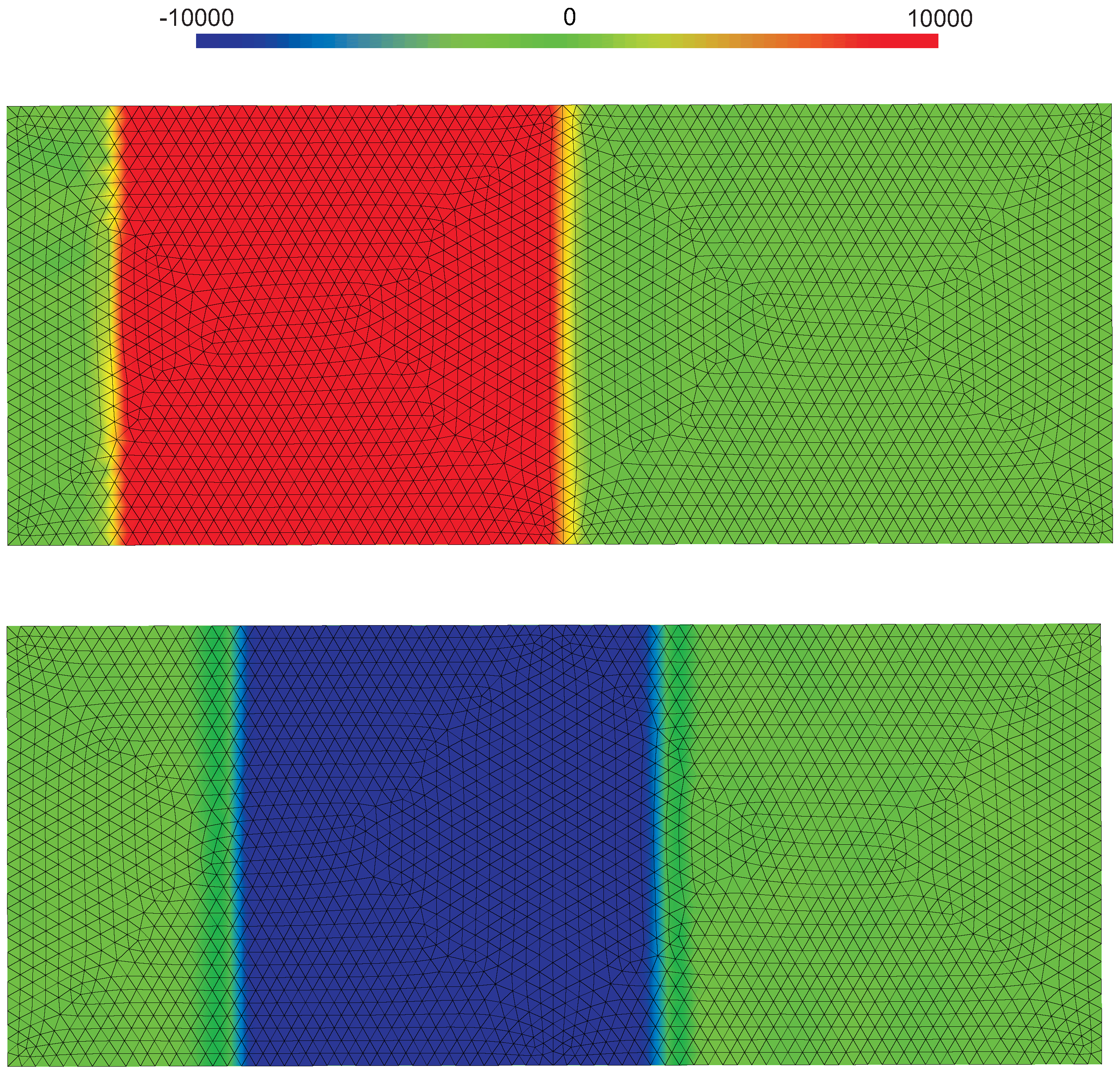
Figure 8. Wave propagating along a homogeneous rod discretized with a two-dimensional unstructured mesh: longitudinal stress field at (top) $t=0.5·{10}^{-2}$ s and (bottom) $t=1.8·{10}^{-2}$ s.

In case of perfect adhesion between the two phases, i.e. in case of $E_{\Gamma }\to \infty$, the exponential terms in (39) and (40) drop to zero. The time-dependent feature of the solution is thus lost in view of the non-evolving microstructure along the interface.

4.2. FE-FCT results

Similarly to what done in [9], all the results to follow have been obtained by adopting: $L=0.5$ m; ${\varrho }_A={\varrho }_B={10}^2$ kg/m${}^3$; $\overline{\tau }={10}^4$ Pa, so as to initially cause the propagation of a tensile wave inside material A of magnitude ${\sigma }_{\text{in}}={10}^4$ Pa; $\Delta t_{\tau }=4·{10}^{-3}$ s. As for the FCT parameters, if not otherwise stated we have adopted: ${\eta }_D={\eta }_A=0.125$ [9], and ${\ell }_{\text{FCT}}=\frac{L}{1000}$.

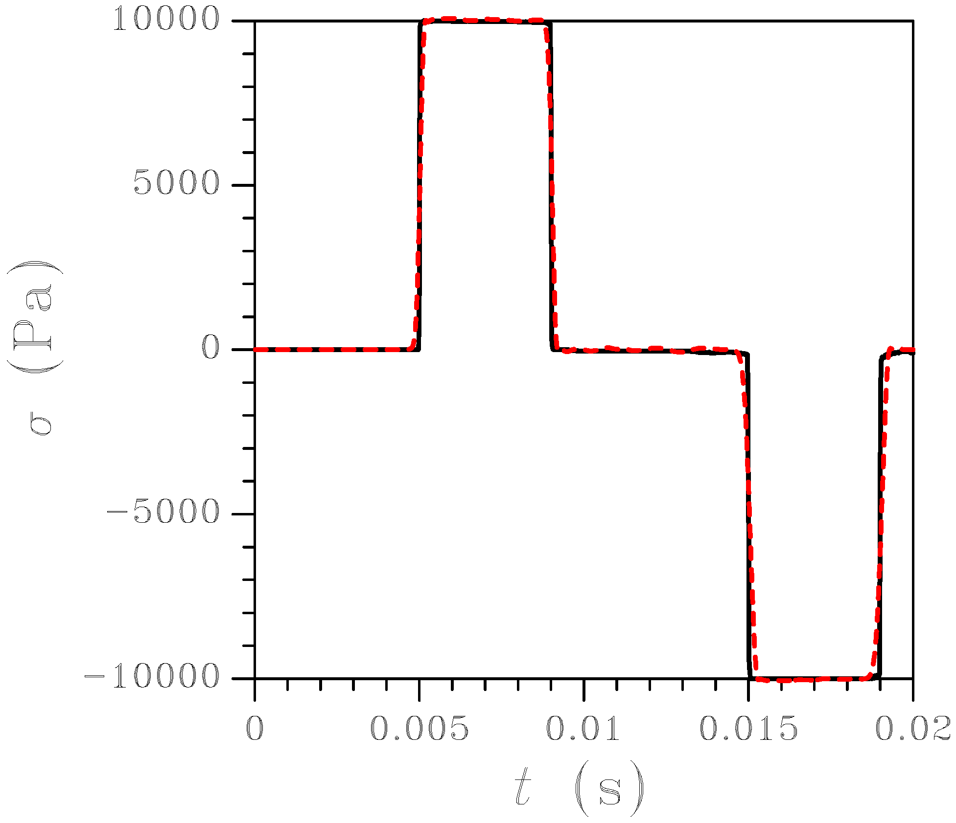
Figure 9. Wave propagating along a homogeneous rod discretized with unstructured meshes: comparison between the evolutions of the longitudinal stress at $x=0.5$ m, as obtained through one-dimensional (black solid line) and two-dimensional (red dashed line) simulations.

Figure 9. Wave propagating along a homogeneous rod discretized with unstructured meshes: comparison between the evolutions of the longitudinal stress at $x=0.5$ m, as obtained through one-dimensional (black solid line) and two-dimensional (red dashed line) simulations.

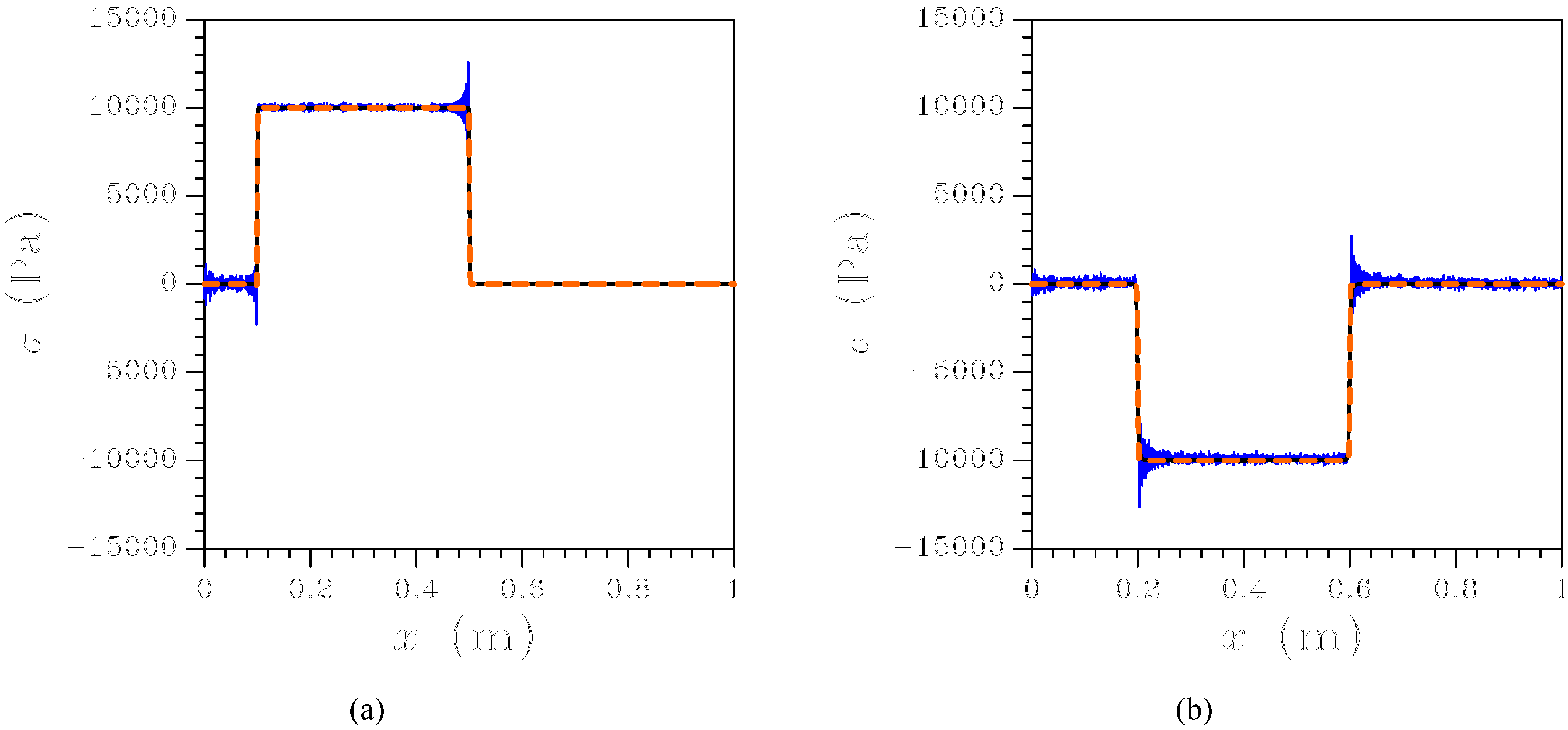
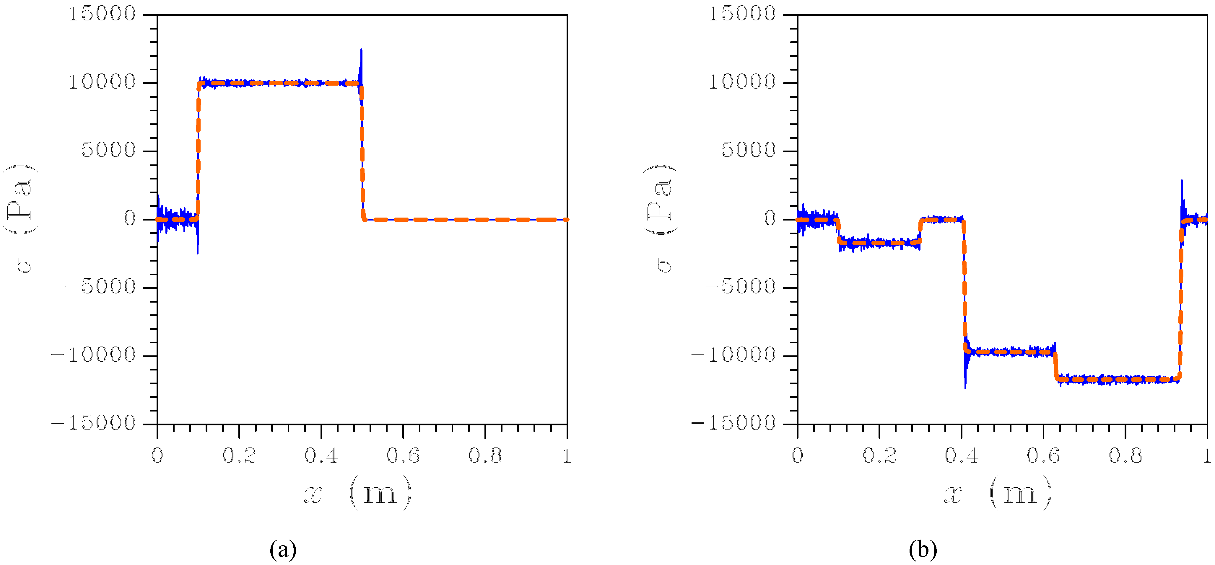
Figure 10. Wave propagating along a heterogeneous rod with perfect bonding between phases, discretized with an unstructured mesh: stress field at (a) $t=0.5·{10}^{-2}$ s and at (b) $t=1.3·{10}^{-2}$ s. Blue solid line: FE solution; orange dashed line: newly proposed FE-FCT solution.

Figure 10. Wave propagating along a heterogeneous rod with perfect bonding between phases, discretized with an unstructured mesh: stress field at (a) $t=0.5·{10}^{-2}$ s and at (b) $t=1.3·{10}^{-2}$ s. Blue solid line: FE solution; orange dashed line: newly proposed FE-FCT solution.

Figure 11. Wave propagating along an interface-containing homogeneous rod ($E_{\Gamma }=5·{10}^7$ N/m${}^3$) discretized with an unstructured mesh: stress field at $t=0.9·{10}^{-2}$ s. Black dotted line: analytical solution; blue solid line: FE solution; orange dashed line: newly proposed FE-FCT solution.

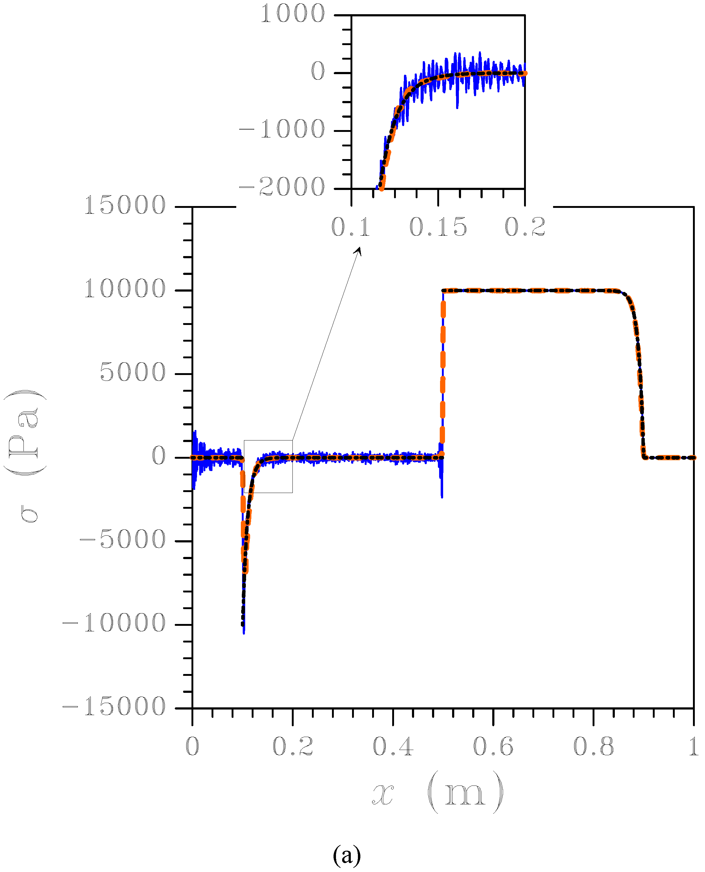
Figure 11. Wave propagating along an interface-containing homogeneous rod ($E_{\Gamma }=5·{10}^7$ N/m${}^3$) discretized with an unstructured mesh: stress field at $t=0.9·{10}^{-2}$ s. Black dotted line: analytical solution; blue solid line: FE solution; orange dashed line: newly proposed FE-FCT solution.

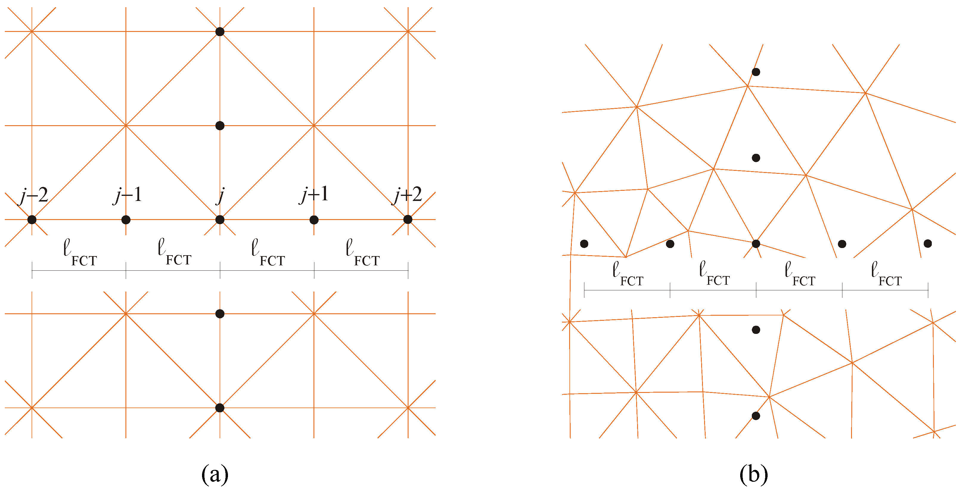
In a first example the rod has been assumed homogeneous, i.e. made of two phases featuring the same Young’s modulus $E_A=E_B={10}^6$ Pa and perfectly bonded together. In the absence of wave reflection along inner surfaces, the present outcomes are meant to assess the robustness of the new FE-FCT scheme when either structured or unstructured space discretizations are adopted. In our analysis, unstructured one-dimensional meshes have been obtained from the relevant structured ones as follows. Starting with a nodal spacing $\Delta x$ (here $\Delta x=5·{10}^{-4}$ m, meaning that 1000 quadratic elements, with characteristic size ${\ell }_e^{1D}=2\Delta x=\frac{L}{500}$, have been adopted to discretize the whole specimen), a random sequence $\text{ran}[-0.50.5]$ is generated so as:

$$\begin{array}{c}\hfill x_{\text{unstruct}}^j=x_{\text{struct}}^j+\chi \Delta x·\text{ran}[-0.50.5]\end{array}$$

(41)

where: $x_{\text{struct}}^j$ and $x_{\text{unstruct}}^j$ are the longitudinal coordinates of the $j-$th node in the structured and unstructured meshes, respectively; $\chi =0.6$ is a scaling factor, introduced to ensure positivity of the length of each element in the unstructured mesh.

Figure 5 shows the stress distribution in the rod at time instants $t=0.5·{10}^{-2}$ s and $t=1.8·{10}^{-2}$ s; it can be seen that the tensile wave, after reflection at the rear free surface of the specimen, becomes a compressive wave of same amplitude. These results have been obtained with a structured mesh, hence the standard [8] and the newly proposed FE-FCT schemes furnish the same outcomes. Moreover, the analytical solution can not be distinguished from the FE-FCT ones; on the other hand, ripples show up in the FE solution, initially just behind the wave fronts (see Figure 5(a), where the discontinuities are propagating from left to right) and eventually spoiling the accuracy of the solution along the whole specimen (see Figure 5(b)).

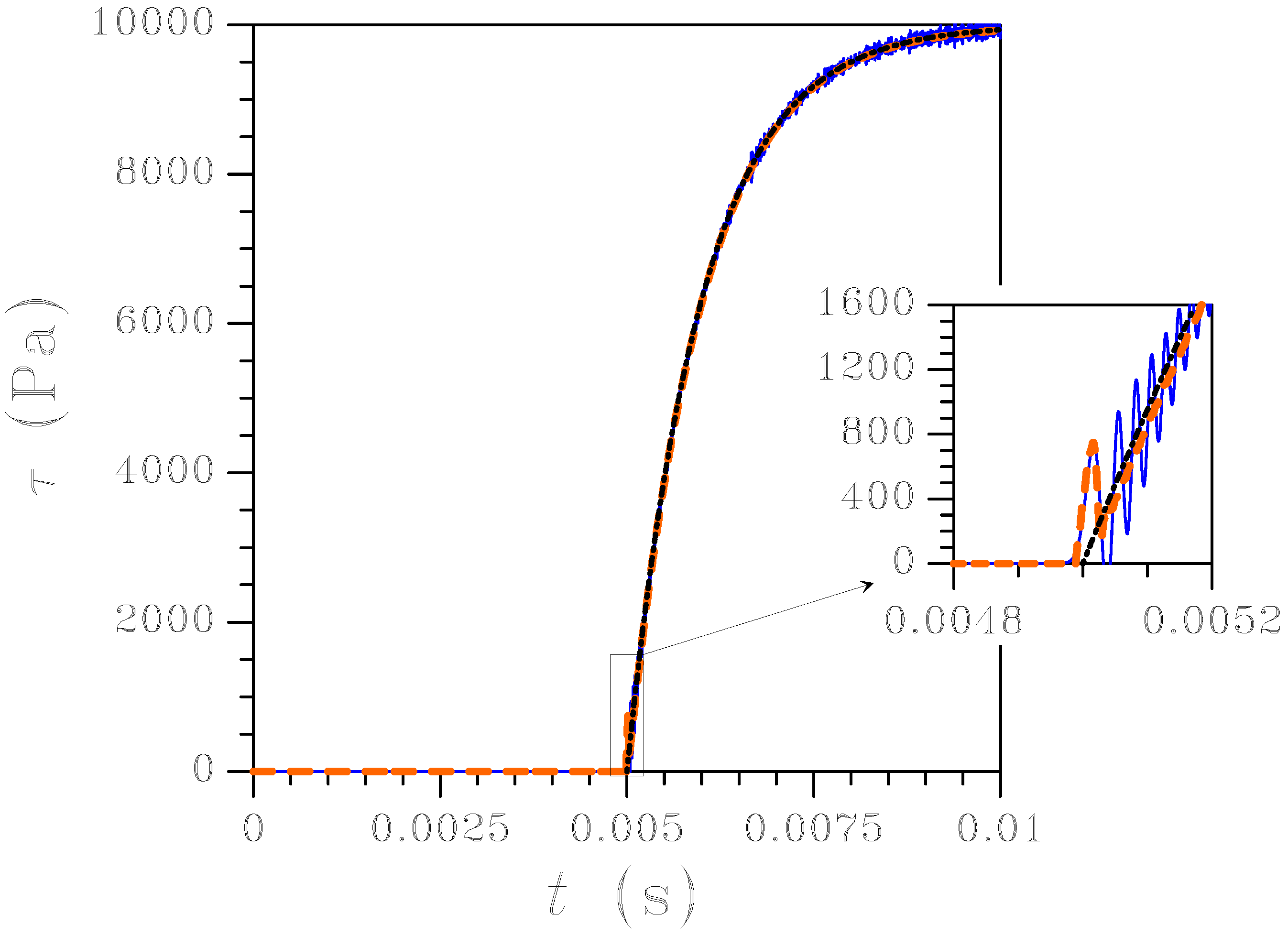
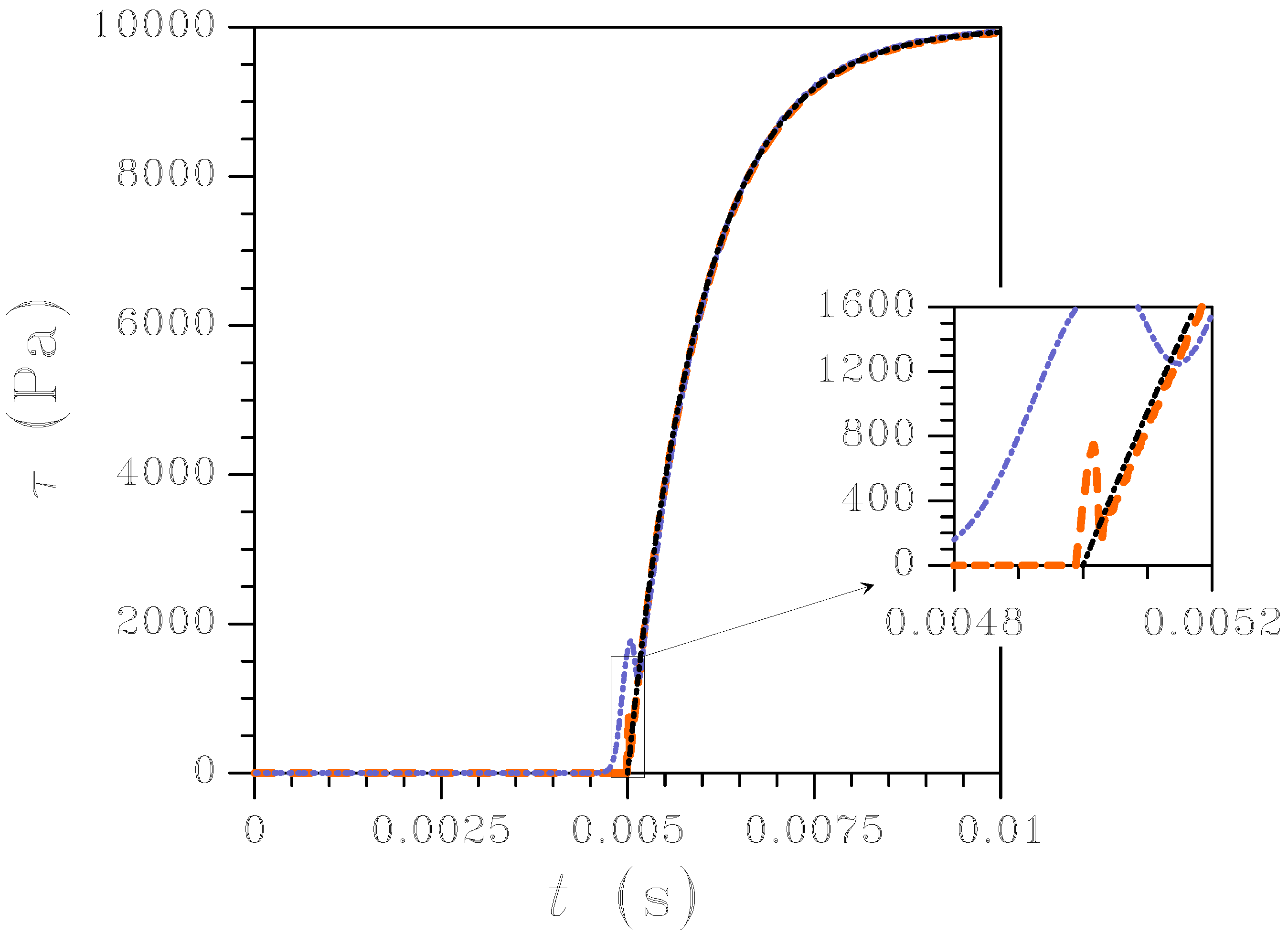
Figure 12. Wave propagating along an interface-containing homogeneous rod ($E_{\Gamma }=5·{10}^6$ N/m${}^3$) discretized with an unstructured mesh: evolution in time of the normal traction τ at the interface. Black dotted line: analytical solution; blue solid line: FE solution; orange dashed line: newly proposed FE-FCT solution.

Figure 12. Wave propagating along an interface-containing homogeneous rod ($E_{\Gamma }=5·{10}^6$ N/m${}^3$) discretized with an unstructured mesh: evolution in time of the normal traction τ at the interface. Black dotted line: analytical solution; blue solid line: FE solution; orange dashed line: newly proposed FE-FCT solution.

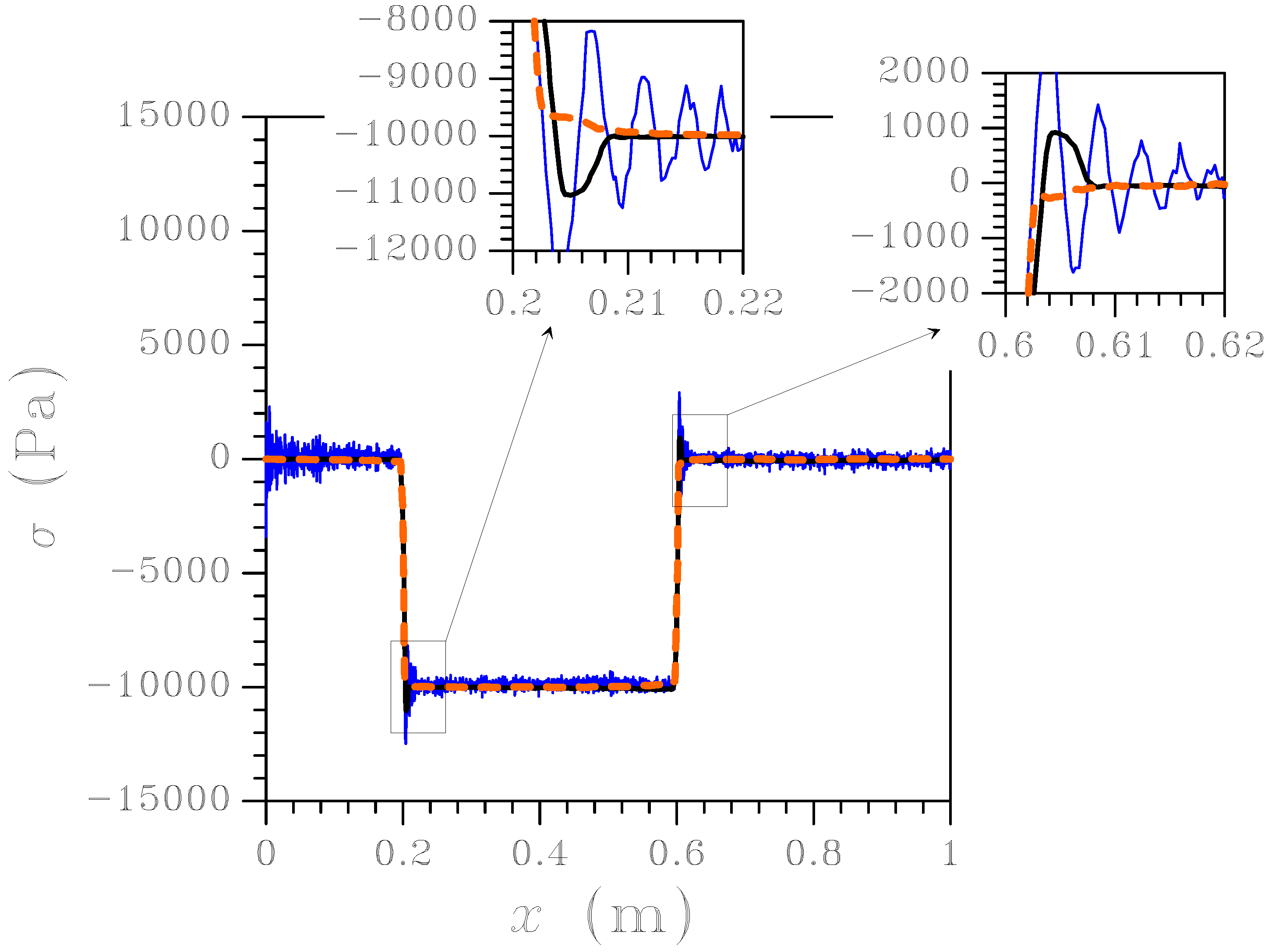
In case of unstructured meshing, the methods here compared furnish the results summarized in Figure 6 in terms of stress field at $t=1.8·{10}^{-2}$ s. As expected, the FE solution wildly oscillates, with ripples of increased amplitude as compared to the structured mesh case; the standard FE-FCT scheme is no more able to fully damp oscillations, whereas the new one works properly and prevents the birth of spurious maxima/minima. It must be noticed that the small delay of the new FE-FCT method in the attainment of the analytical solution (characterized by sharp discontinuities), as shown in the two insets of Figure 6, may be avoided or reduced in duration by a fine tuning of Newmark parameters β, γ and FCT parameters ${\eta }_D$, ${\eta }_A$. To prove it, Figure 7 shown the effect of ${\eta }_D={\eta }_A$ on the aforementioned delay; as far as this feature of the solution is concerned, it can be seen that smaller parameter values strongly reduce the delay, even if the value of the longitudinal stress may get affected. Only results relevant to ${\eta }_D={\eta }_A$ are here reported; on the one hand, if ${\eta }_D>{\eta }_A$ the solution is characterized by an excessive diffusion around the discontinuities, with fronts smeared over too many FEs; on the other hand, if ${\eta }_D<{\eta }_A$ the solution has a tendency to instability, characterized by ripple amplitudes continuously increasing in time.

For comparison purposes, outcomes of a two-dimensional simulation are depicted in Figure 8 in terms of contour plots of the longitudinal stress before (Figure 8(a)) and after (Figure 8(b)) reflection at the rear free surface. In this two-dimensional case a much coarser space discretization has been adopted, with 6-node triangular elements featuring a characteristic size ${\ell }_e^{2D}=\frac{L}{100}$. It can be seen that the stress wave maintain sharp fronts, always perpendicular to the propagation direction independently of local mesh features. Because of the coarse discretization, it is expected that spurious oscillations are here characterized by an increased amplitude when compared to the one-dimensional case. Figure 9, where the time history of the longitudinal stress at $x=0.5$ m is reported, testifies the performance of the proposed FE-FCT scheme: even though the ratio between the characteristic sizes of FEs is $\frac{{\ell }_e^{1D}}{{\ell }_e^{2D}}=5$, the discrepancy between the two solutions amounts at most to 2%.

Figure 13. Wave propagating along an interface-containing homogeneous rod ($E_{\Gamma }=5·{10}^6$ N/m${}^3$) discretized with one-dimensional and two-dimensional unstructured meshes: evolution in time of the normal traction τ at the interface. Black dotted line: analytical solution; orange dashed line: one-dimensional FCT-FE solution; blue dotted line: two-dimensional FCT-FE solution.

Figure 13. Wave propagating along an interface-containing homogeneous rod ($E_{\Gamma }=5·{10}^6$ N/m${}^3$) discretized with one-dimensional and two-dimensional unstructured meshes: evolution in time of the normal traction τ at the interface. Black dotted line: analytical solution; orange dashed line: one-dimensional FCT-FE solution; blue dotted line: two-dimensional FCT-FE solution.

In a second example, to start assessing the efficiency of the FE-FCT scheme in the presence of inner boundaries, it has been assumed that $E_B=2·{10}^6$ Pa at fixed values of all the other material parameters; perfect adherence between the two phases was also assigned. FE and FE-FCT results are shown in Figure 10 in terms of stress field at $t=0.5·{10}^{-2}$ s and $t=1.3·{10}^{-2}$ s. At $t=0.5·{10}^{-2}$ s (Figure 10(a)), since the leading front of the stress wave has not impinged yet upon the interface (placed at $x=0.5$ m) the results are similar to those of Figure 5(a), showing again that the FCT scheme properly damps oscillations (as before, the analytical solution is not reported here since it can not be distinguished from the FE-FCT one). Moreover, when waves are partially reflected by the inner surface the solution still proves accurate, even without explicitly accounting for the acoustic impedance of each phase as done in [9].

In a third example, the behavior of a homogeneous two-phase specimen ($E_A=E_B={10}^6$ Pa) containing a compliant interface has been studied. In the case $E_{\Gamma }=5·{10}^7$ N/m${}^3$, results in terms of the stress field at $t=0.9·{10}^{-2}$ s are depicted in Figure 11; even in the presence of a compliant interface, it can be seen that the new FE-FCT method correctly reproduces the response of the body without spurious oscillations. To further assess the accuracy of the method, the time history of the normal traction τ across Γ is shown in Figure 12. To increase the duration of the transitory stage and to get insights into the performance of the FE-FCT method, the interface stiffness has been decreased to $E_{\Gamma }=5·{10}^6$ N/m${}^3$, and the loading interval $\Delta t_{\tau }$ has been slightly increased accordingly, so as to ensure completion of interface opening till ${\left[u\right]}^{☆}=\frac{\overline{\tau }}{E_{\Gamma }}$. Once again, the FE solution looks oscillatory; this behavior becomes a serious issue in case of nonlinear, irreversible interface modes, since spurious unloadings and overshoots may cause a drift of the computed solution away from the exact one. The FE-FCT solution instead presents only an oscillation just after the leading front of the stress wave has impinged upon the interface; afterwards, the FCT scheme filters out possible subsequent ripples. This is also shown in Figure 13, where results of one-dimensional and two-dimensional simulations are compared; in the two-dimensional case, the same space discretization depicted in Figure 8 has been adopted. According to previous results, the higher oscillation amplitude around $t=0.005$ s in the two-dimensional simulation is caused by the coarser mesh; subsequently, the FCT scheme completely damps ripples.

The small time discrepancy (amounting to $\Delta t^{☆}\cong {10}^{-5}$ s in the one-dimensional case) between FE-FCT and exact solutions is due to the dispersive properties of the FE solution and can be explained as follows. While the analytical solution is characterized by sharp wave fronts, in the FE-FCT one discontinuities are smeared over the resolved length-scale, which is typically one element wide; $\Delta t^{☆}$ is about the time interval required by the stress wave to travel across $\Delta x$ (or the corresponding node spacing in the unstructured mesh case) at speed $c_A=c_B$.

5. Concluding remarks

In this paper we have proposed a finite element flux-corrected transport (FE-FCT) method for the simulation of stress wave propagation in homogeneous as well as heterogeneous bodies.

Through a comparative assessment of existing remedies for the oscillatory behavior of standard FE simulations of moving discontinuities, the FCT algorithm emerged as a very promising tool. It consists of post-processing the velocity field, as furnished by a customary FE scheme, via diffusive and antidiffusive fluxes, the latter being appropriately limited in size. The main limitations of present implementations, already foreseen e.g. in [8,9], are the need of structured space discretizations, which entails an ad-hoc treatment of irregular boundaries of the body, and the former knowledge of the acoustic impedance of each phase in case of waves traveling inside heterogeneous bodies. This second issue prevents the simulation of the dynamics of polycrystals (i.e. highly heterogeneous solids) in the presence of defective, compliant interphase boundaries, since acoustic impedances turn out to be influenced by the interphase compliances and by the angle between the wave propagation direction and each phase boundary. We have here proposed a new FCT scheme, which is able to deal with irregular and compliant phase boundaries; this new scheme relies upon an algorithmic length-scale, used to define the size of the nodal support within which the velocity field is corrected through the diffusive/antidiffusive fluxes. Close to phase boundaries, alike close to boundaries of the whole body, the aforementioned local support is properly re-shaped: this permits to account for possible interphase compliances.

Through one-dimensional and two-dimensional simulations of stress waves propagating along slender bodies (rods), it has been shown that the newly proposed FE-FCT method is effective and robust. Results, never showing macroscopic fluctuations in the stress and velocity fields, turned out to be very accurate when compared to available analytical solutions, and independent of the (unstructured) space discretizations adopted.