An Unknown Radar Emitter Identification Method Based on Semi-Supervised and Transfer Learning

Abstract

Aiming at the current problem that it is difficult to deal with an unknown radar emitter in the radar emitter identification process, we propose an unknown radar emitter identification method based on semi-supervised and transfer learning. Firstly, we construct the support vector machine (SVM) model based on transfer learning, using the information of labeled samples in the source domain to train in the target domain, which can solve the problem that the training data and the testing data do not satisfy the same-distribution hypothesis. Then, we design a semi-supervised co-training algorithm using the information of unlabeled samples to enhance the training effect, which can solve the problem that insufficient labeled data results in inadequate training of the classifier. Finally, we combine the transfer learning method with the semi-supervised learning method for the unknown radar emitter identification task. Simulation experiments show that the proposed method can effectively identify an unknown radar emitter and still maintain high identification accuracy within a certain measurement error range.

1. Introduction

Radar emitter identification is the key link in radar reconnaissance. It extracts the characteristic parameters and working parameters on the basis of radar signal sorting. Based on these parameters, we can obtain the information such as the system, use, type and platform of the target radar, and further deduce the battlefield situation, threat level, activity rule, tactical intention, etc., and provide important intelligence support for one’s own decision-making [1]. The most commonly used radar emitter identification method is the pulse described word-based method. As new radar systems are born, and the radar is becoming more complex, the method is difficult to cope with the complex electromagnetic environment of modern battlefields. In order to obtain better identification results, researchers began to extract a variety of new features in the time domain [2], frequency domain [3] and time-frequency domain [4] for the identification of radar emitters.

With the rise of deep learning techniques, more and more researchers have applied CNN and DBN in the radar emitter identification task, which achieves good performance. Zhou Z et al. [5] developed a novel deep architecture for automatic waveform recognition, which outperformed the existing shallow algorithms and other hand-crafted, feature-based methods. Cain L et al. [6] investigated an application of convolutional neural networks (CNN) for rapid and accurate classification of electronic warfare emitters. Sun J et al. [7] proposed a deep learning model named as unidimensional convolutional neural network (U-CNN) to classify the encoded high-dimension sequences with big data.

Kong M et al. [8] used the CNN deep learning algorithm to identify the radar radiation sources, which could extract more detailed features of the radar and improve the recognition rate. To cope with the complex electromagnetic environment and varied signal styles, Wang X et al. [9] proposed a novel method based on the energy cumulant of short time Fourier transform and reinforced deep belief network to gain a higher correct recognition rate for radar emitter intra-pulse signals at a low signal-to-noise ratio.

In the past battlefields, the types of radar emitters are single and limited, and the above methods can solve the problem of radar emitter identification well. However, with the increasing number and variety of radar emitters, many unknown emitters will appear in the future battlefield. As time goes by and the location changes, the current identification methods will face two problems. First, the training data and testing data no longer satisfy the same-distribution hypothesis, resulting in a decrease in the classification performance of the machine learning model. Second, the number of available labeled samples for unknown emitters is seriously insufficient, which may lead to over-fitting of the machine learning model.

In recent years, the transfer learning methods [10] and the semi-supervised learning methods [11] have gained more and more attention. Transfer learning does not require that the training data and testing data meet the conditions of the same distribution in the model training process, and utilizes the knowledge in a large number of known samples for training, which is good for cross-domain learning. However, the transferring of a large amount of irrelevant information will also cause negative transfer, which reduces the effect of identification. Semi-supervised learning can use the information in a small number of labeled samples and find patterns from a large number of unlabeled samples, and then perform classification, avoiding the use of only a small number of labeled samples for training, which may result in over-fitting. However, as information continues to increase, the training data and testing data will also not satisfy the same-distribution hypothesis.

In view of the different characteristics of transfer learning and semi-supervised learning, this paper combines the two methods to propose an unknown radar emitter identification method based on semi-supervised and transfer learning. Firstly, we construct the support vector machine model based on transfer learning, using the information of labeled samples in the source domain to train in the target domain, which can solve the problem that the training data and the testing data do not satisfy the same-distribution hypothesis. Then we design a semi-supervised, co-training algorithm, using the information of unlabeled samples to enhance the training effect, which can solve the problem that insufficient labeled data results in inadequate training of the classifier. Finally, we combine the transfer learning method with the semi-supervised learning method for the unknown radar emitter identification task.

Our major contributions are summarized as follows: (1) Focusing on the actual application scenarios to study radar emitter identification, and simultaneously solving the problem that training data and testing data do not satisfy the same-distribution hypothesis and the problem of insufficient labeled data, which provides a good thinking way for future research in this area; (2) proposing a method combining support vector machine based on transfer learning with semi-supervised co-training algorithm; (3) verifying the interaction between the transfer learning method and the semi-supervised learning method for unknown radar emitter identification task.

2. Relevant Research

2.1. Transfer Learning

Transfer learning refers to learning the knowledge in the source domain $D_s$, and using in the target domain $D_t$ that is not the same distribution with $D_s$ but is related to $D_s$, which makes good the problem of insufficient training data. Unlike traditional machine learning methods, transfer learning [12] does not require training data and testing data to satisfy the same-distribution hypothesis. It can discover and extract knowledge in the source domain $D_s$ that matches the distribution of the target domain $D_t$ and is useful for identification in the target domain $D_t$.

Then it establishes classification models in the target domain $D_t$, which can make efficient use of existing labeled samples to avoid re-labeling in the target domain $D_t$.

From the perspective of transfer methods, transfer learning includes four basic methods: sample-based transfer [13], feature-based transfer [14], model-based transfer [15] and relationship-based transfer [16]. The sample-based transfer method refers to producing rules according to certain weights, and reusing data samples for transfer learning. The feature-based transfer method refers to mutual transfer by feature transformation, which reduces the gap between the source domain and the target domain, or transforms the data features of the source domain and the target domain into a unified feature space, and then utilizes the traditional machine learning methods for identification. The model-based transfer method refers to finding the parameter information shared between the source domain and the target domain to implement transferring. The relationship-based transfer method has a completely different approach from the above three methods, focusing on the similarity between the source domain samples and target domain samples.

2.2. Semi-Supervised Learning

The commonly used machine learning methods can be divided into three categories: supervised learning, unsupervised learning and semi-supervised learning. Supervised learning refers to only using labeled samples for training, and may not obtain a model with high generalization ability in the case of fewer labeled samples. Unsupervised learning refers to only using unlabeled samples for training, regardless of labeled samples, which results in a waste of samples. Semi-supervised learning can process a small number of labeled samples and a large number of unlabeled samples at the same time, combining the advantages of supervised learning and unsupervised learning.

The four most commonly used algorithms for semi-supervised learning are Self-Training [17], Co-Training [18], Generative Model [19] and Graph-Based Semi-supervised [20]. The Self-Training algorithm refers to the use of a self-classifier to continuously generate high-confidence samples for improving the final classification performance. The Co-Training algorithm refers to separately training the classifier on two views, which is representative of multi-view learning. The Generative Model-based method means that the data of different categories meets different distributions, and if its conditional probability distribution is known, the parameters of the model can be solved. The Graph-Based, Semi-supervised method refers to passing the label information of labeled samples to unlabeled samples according to the adjacency relationship in the graph, thereby realizing the classification of the unlabeled samples.

3. Unknown Radar Emitter Identification Based on Semi-Supervised and Transfer Learning

In this section, we use the support vector machine model as the base classifier. Firstly, we construct the support vector machine based on transfer learning, and define the calculation index to measure the transfer ability. Then we study the training effect enhancement method based on the semi-supervised co-training algorithm. Finally, we combine the transfer learning method with the semi-supervised learning method for the unknown radar emitter identification task.

3.1. Support Vector Machine Based on Transfer Learning

The support vector machine (SVM) model has the characteristics of simple structure and global optimization, and is good at solving small sample and nonlinear problems. Therefore, this section chooses the support vector machine model as the base classifier to perform radar emitter identification.

In the process of constructing the SVM model based on transfer learning, it is necessary to utilize the data in two domains at the same time, namely source domain $D_s$ and target domain $D_t$. The data in source domain $D_s$ refers to the known radar emitters that are detected during non-wartime, and the data in target domain $D_t$ refers to the emerging radar emitters in wartime.

When the amount of data in source domain $D_s$ is large, noise in source domain $D_s$ affects the use of the data in target domain $D_t$.

In order to better optimize the target equation, this section filters the data with high similarity in the source domain $D_s$ in the process of transferring the SVM model, and uses the Euclidean distance to define the distance function $\sigma (V_s^i,D_t^j)$, which can measure the similarity between the source domain data and the target domain data. Its formula is as follows:

$$\sigma (V_s^i,D_t^j)=-\frac{1}{k}{\displaystyle \sum _{(x_j,y_j)\in D_t}\exp \{-\beta \parallel V_s^i-x_j{\parallel }_2^2\}}$$

(1)

where $V_s^i$ is the support vector for source domain, $\beta$ is the importance degree of $V_s$, $(x_j,y_j)$ is the sample in target domain $D_t$ and its real category, $\parallel V_s^i-x_j{\parallel }_2^2$ is the Euclidean distance between $V_s$ and $D_t$, k is the number of samples in target domain $D_t$.

The specific steps of the support vector machine based on transfer learning are shown in Algorithm 1.

Algorithm 1. Support vector machine based on transfer learning Train the initial SVM model in the source domain $D_s$ to get the support vector $V_s$, and calculate the similarity distance function $\sigma (V_s^i,D_t^j)$. Add $V_s$ to the source domain data, and add the similarity distance function $\sigma$ to the objective function of the SVM model as follows: $\underset{w}{\min }0.5\parallel w{\parallel }_2^2+C{\displaystyle \sum _{j=1}^k{\epsilon }_j}+{\displaystyle \sum _{i=1}^m\sigma (V_s^i,D_t^j){\overline{\epsilon }}_i}$ Where m is the number of samples in source domain $D_s$, C is the penalty term, w is the weights of classification hyperplane in the SVM model. Generate new training set $\tilde{D}$ in target domain $D_t$, and retrain the SVM model. The optimization problem of the objective function is described with the Lagrangian coefficient as follows: $\max L(\alpha )={\displaystyle \sum _{i=1}^{m+k}{\alpha }_i}-0.5{\displaystyle \sum _{i=1}^{m+k}{\displaystyle \sum _{j=1}^{m+k}{\alpha }_i{\alpha }_j{y}_i{y}_j(x_i\ast x_j)}}$ Where $x_i\ast x_j$ is the inner product of the vector $x_i$ and the vector $x_j$, $y_i$ is the real category label of $x_i$, $y_j$ is the real category label of $x_j$, ${\alpha }_i$ and ${\alpha }_j$ are the Lagrangian multipliers, $\alpha ={({\alpha }_1,{\alpha }_2,\cdots ,{\alpha }_{m+k})}^T$ is the Lagrangian multiplier vector. Solve the above optimization problem and get the optimal solution ${\alpha }^{\ast }$, which means getting the final SVM model. Its form is as follows: $f(x)=sign[{\displaystyle \sum _{j=1}^{m+k}{y}_i{\alpha }^{\ast }(x_i\ast x_j)}+y_i-{\epsilon }_i-{({\displaystyle \sum _{i=1}^{m+k}{\alpha }^{\ast }{x}_i{y}_i})}^T{x}_i]$

3.2. Transfer Ability

The transfer ability can reflect the influencing ability of the samples in source domain $D_s$ on the target domain $D_t$. The calculation process involves two important indices: the similarity between the sample in source domain $D_s$ and the sample in target domain $D_t$; the consistency between the prediction result of the sample $x_i$ in the classifier f and its real category. Therefore, the calculation formula of transfer ability is as follows:

$${\alpha }_i=\sigma (V_s^i,D_t^j)\ast 〚f(x_i)==y_i〛$$

(2)

where $\sigma (V_s^i,D_t^j)$ is the similarity distance function, f is the SVM classifier trained by the above transfer learning method, $f(x_i)$ is the predicted value of $x_i$ in source domain $D_s$ by the classifier f, $y_i$ is the real category label of $x_i$. By calculating the transfer ability, it is helpful to select the samples in source domain $D_s$ which are related to target domain $D_t$.

3.3. Training Effect Enhancement Based on Semi-Supervised Co-Training Algorithm

The transfer learning-based support vector machine can select the appropriate samples from source domain $D_s$ for the training on target domain $D_t$, which can improve the final identification performance. Unlike the above, semi-supervised learning can use the unlabeled samples in target domain $D_t$ to enhance the final training effect. This section constructs the semi-supervised co-training algorithm based on the base classifier SVM model. The specific steps are shown in Algorithm 2.

Algorithm 2. Semi-supervised co-training algorithm For the radar emitter identification task, define and construct a feature set $x$, and divide it into two parts $x_1$ and $x_2$. Train the base classifier SVM model on the small number of labeled samples in target domain $D_t$ by using the feature sets $x_1$ and $x_2$ respectively, and obtain the classifiers $f_1$ and $f_2$. For t = 1: N Perform identification on the unlabeled samples in target domain $D_t$ by using the classifiers $f_1$ and $f_2$, respectively, and obtain the posterior probabilities of the samples belonging to each emitter category, and select p samples with the highest confidence for each category; Add the selected samples to the training set and retrain the classifiers $f_1$ and $f_2$ on the training set. End

The two feature sets $x_1$ and $x_2$ in the co-training algorithm refer to two views and need to satisfy sufficient redundancy and conditional independence. Through continuous iterative training, unlabeled samples in the target domain $D_t$ are available for labeling, which helps to enhance the training effect.

3.4. Combination of Transfer Learning Method and Semi-Supervised Learning Method

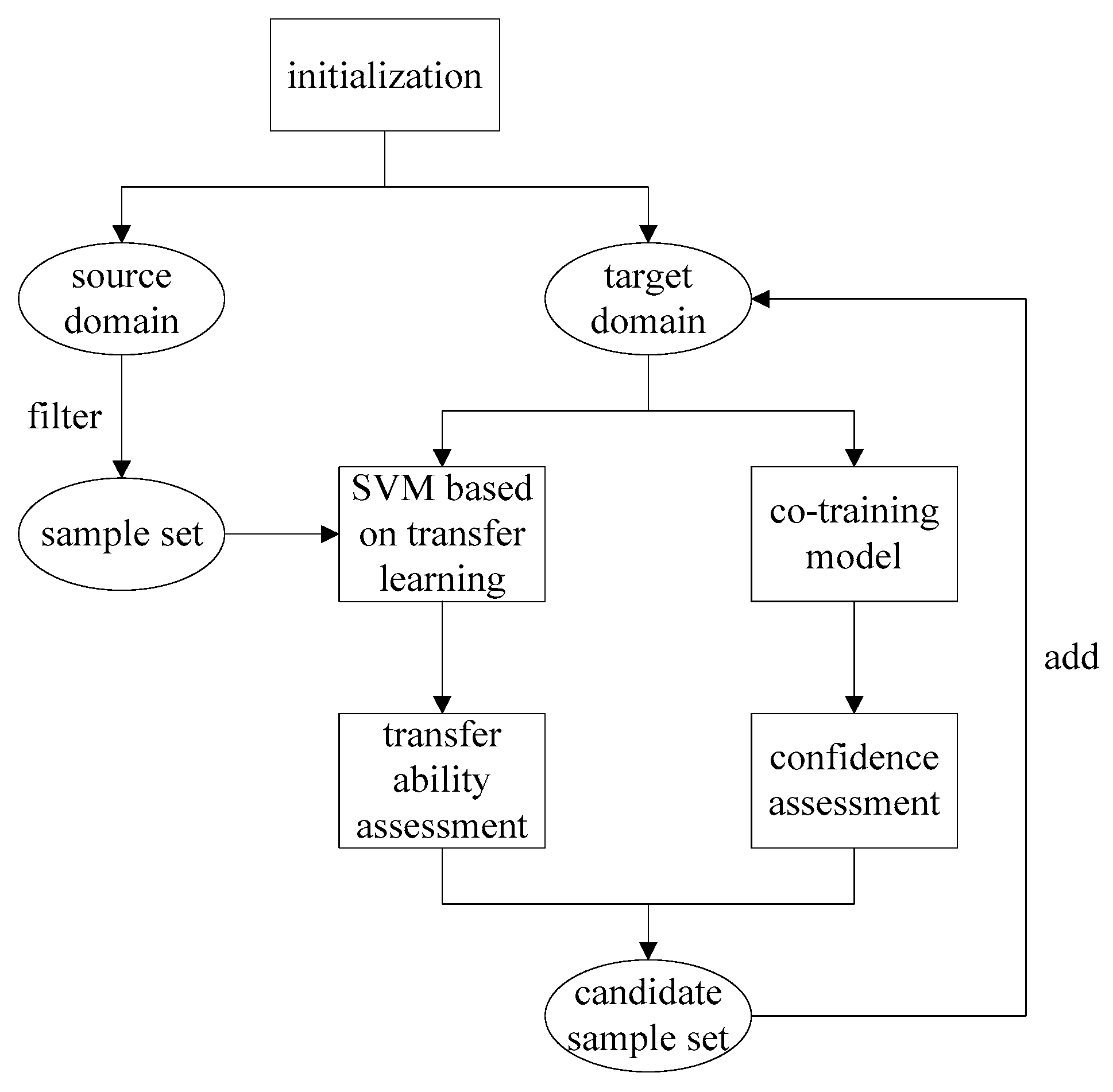
This section combines the transfer learning method with the semi-supervised learning method, while taking advantage of the two methods, which can use useful information in source domain $D_s$ for cross-domain learning, and can enhance the training effect with unlabeled samples in target domain $D_t$. The specific process is shown in Figure 1.

The basic idea of the semi-supervised transfer learning algorithm is to first use the small number of labeled samples in the target domain as training data to train two different classification models, namely the SVM model based on transfer learning and the semi-supervised co-training model; then we select some samples from source domain, use the SVM model based on transfer learning to evaluate the transfer ability of each sample, delete the samples that are not related to the target domain and obtain candidate sample set. After this we select some unlabeled samples from the target domain, use the semi-supervised co-training model to evaluate the confidence of each sample, delete the samples with lower confidence and add the remaining samples to the candidate sample set.

In the process of selection training samples, not only must we consider the transfer ability, but we must assess the confidence of the sample’s category. Then we add the samples satisfying the conditions to the training set. The above sample selection method is based on the basic assumptions of transfer learning and semi-supervised learning. By repeating the process, the number of labeled samples in target domain $D_t$ can be continuously increased.

4. Experiments

4.1. Experiment Settings

4.1.1. Experiment Environment

We build the simulation experiment development environment of Windows7 + Matlab2017b + Libsvm3.22, where Libsvm3.22 is used to implement the SVM model as the base classifier. Its kernel function is based on the radial basis function $\exp (-\frac{|x-x_i{|}^2}{{\sigma }^2})$. On this basis we use Matlab to realize the transfer learning and semi-supervised learning method in this paper.

4.1.2. Experiment Data

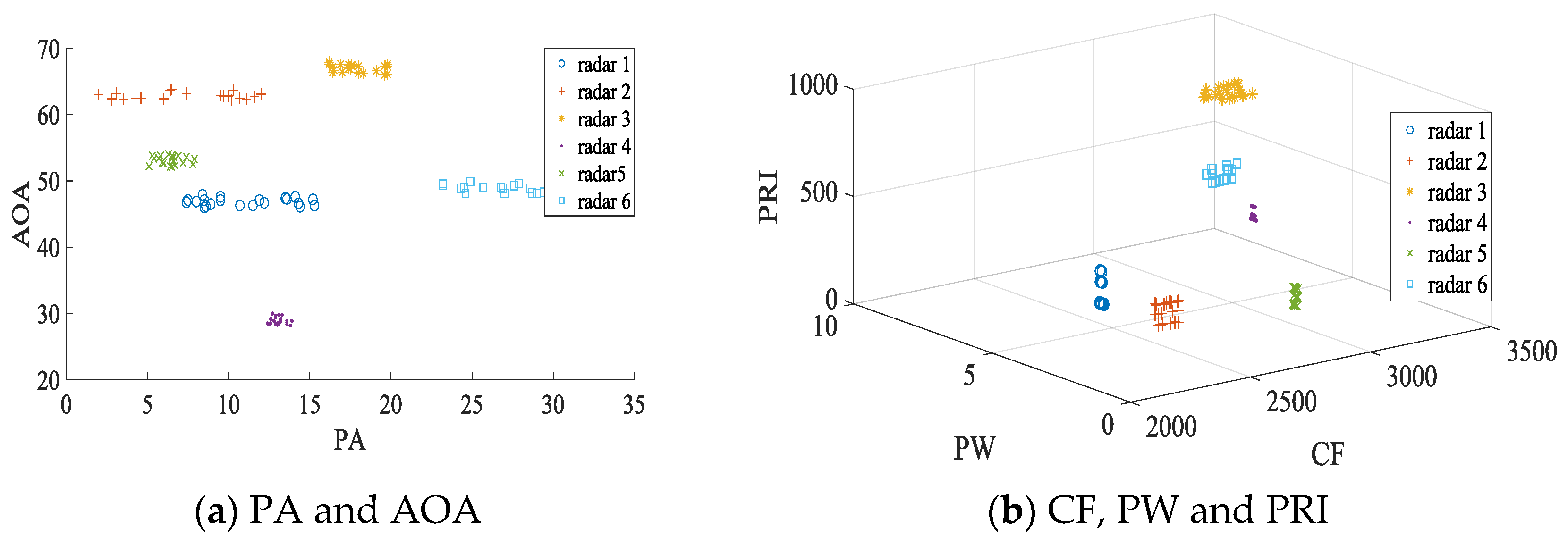
We use the characteristic parameters such as pulse amplitude(PA), carrier frequency (CF), pulse width (PW), pulse repetition interval (PRI) and angle of arrival (AOA) to simulate generating the emitter data of six system-like radars. For the signal parameters, they are set at the same intermediate frequency: 10 MHz, and the sampling frequency is 100 MHz. 1000 signal samples are generated using the above five pulse description words for radar 1, radar 2 and radar 3, respectively, and a total of 3000 signal samples are as known radar emitter data corresponding to the source domain data above.

In addition, 1000 signal samples are generated for radar 4, radar 5 and radar 6, respectively, and a total of 3000 signal samples are as unknown radar emitter data corresponding to the target domain data above. The mean values and standard deviations after normalization of the known radar emitter data and the unknown radar emitter data are significantly different, so they no longer satisfy the assumption of the same distribution, which can be used to verify the transfer learning and semi-supervised learning method. The details of the experiment data are shown in

Table 1. Known radar emitter data.

Known Radar	PA	CF/MHz	$\mathbf{PW}/\mathit{\mu }\mathit{s}$	$\mathbf{PRI}/\mathit{\mu }\mathit{s}$	$\mathbf{AOA}/°$
radar 1	[6, 16]	[2019, 2020]	[1.1, 1.3]	400/500/550	[46, 48]
radar 2	[2, 12]	[2150, 2250]	[0.3, 0.5]	300/350/400	[62, 64]
radar 3	[16, 20]	[3121, 3333]	[7.1, 7.2]	800/830/860	[66, 68]

and

Table 2. Unknown radar emitter data.

Unknown Radar	PA	CF/MHz	$\mathbf{PW}/\mathit{\mu }\mathit{s}$	$\mathbf{PRI}/\mathit{\mu }\mathit{s}$	$\mathbf{AOA}/°$
radar 4	[12, 14]	[2545, 2546]	[0.2, 0.4]	710/730/770	[28, 30]
radar 5	[5, 8]	[2763, 2773]	[0.6, 0.8]	240/280/320	[52, 54]
radar 6	[23, 31]	[2855, 3003]	[4.7, 4.8]	600/640/660	[48, 50]

.

A radar signal sample is written as $W_i={[P{A}_i,C{F}_i,P{W}_i,PR{I}_i,AO{A}_i]}^T$. The distribution of the specific parameters of the radar is shown in Figure 2, (a) describes the entire data set from the perspective of parameters PA and AOA, and (b) describes the entire data set from the perspective of parameters of CF, PW and PRI.

4.2. Interaction between Transfer Learning Method and Semi-Supervised Learning Method

The experiment uses the known radar emitter data as labeled samples for auxiliary training, and the unknown radar emitter data as unlabeled samples to be identified. The number of unlabeled samples and labeled samples can be adjusted to verify the interaction between the transfer learning method and the semi-supervised learning method.

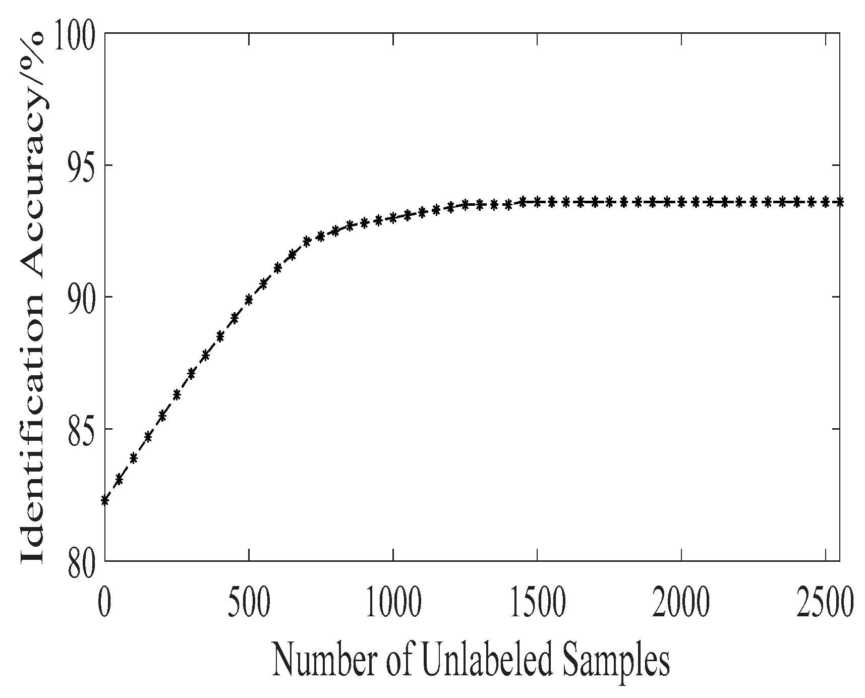
First, we keep the number of labeled samples unchanged, and adjust the number of unlabeled samples to verify the impact of the semi-supervised learning method on the transfer learning method. The results are shown in Figure 3. It can be seen from the experiment results that when the number of unlabeled samples is zero, that is, we only carry out transfer learning without semi-supervised learning, the identification accuracy is 11.3% lower than the optimal identification accuracy.

When the number of unlabeled samples is slowly increasing, the identification accuracy will also continue to rise, indicating that the unlabeled samples help to make the transfer learning method select high-similarity samples from the unknown radar emitter data; that is, the semi-supervised learning method is positively correlated with the transfer learning method, and has not weakened it. As the number of unlabeled samples increases further, the identification accuracy will gradually stabilize, indicating that the high-similarity samples in the unknown radar emitter data have been completely screened out, and the optimal recognition rate can reach 93.6%.

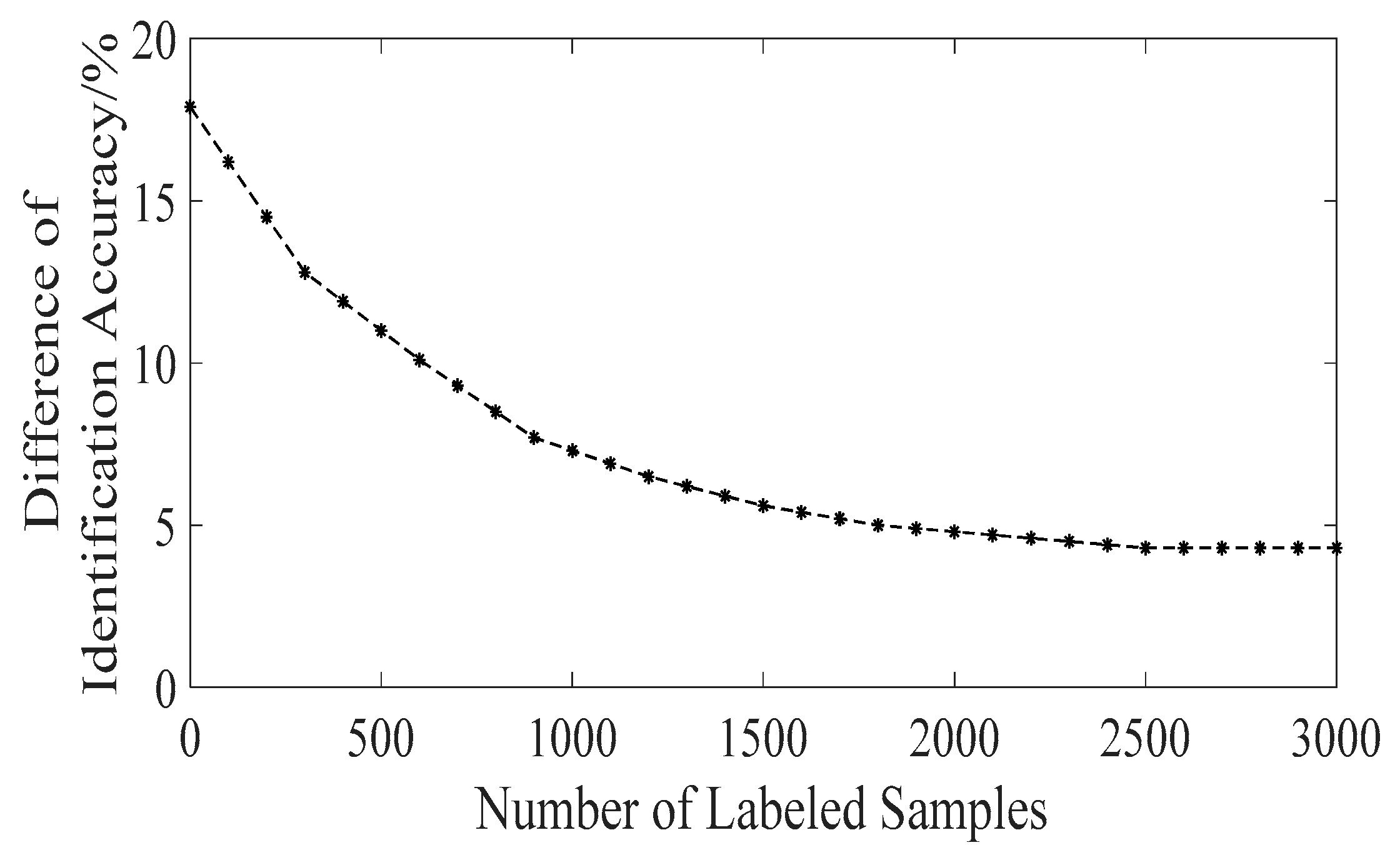
Secondly, we keep the number of unlabeled samples unchanged, and adjust the number of labeled samples to verify the impact of the transfer learning method on the semi-supervised learning method. The results are shown in Figure 4. It can be seen from the experiment results that when the number of labeled samples is zero, that is, we only carry out semi-supervised learning without transfer learning, the difference between the maximum identification accuracy and the minimum identification accuracy in the classification identification results reaches 17.9%, indicating that the use of semi-supervised learning alone makes the model less stable. When the number of labeled samples is slowly increased, the difference between the maximum identification accuracy and the minimum identification accuracy in the classification identification results will continue to drop to 4.3%, indicating that the transfer learning method helps to make self-correction of the semi-supervised learning method.

It can be seen from the above experiment results that the semi-supervised and transfer learning method proposed in this paper can comprehensively utilize the information of unlabeled samples and labeled samples. When the number of unlabeled samples is greater than 1000, and the number of labeled samples is greater than 1500, the performance of the model will tend to be stable and achieve the highest identification accuracy. Therefore, in the following we use 1500 known radar emitter samples and 1000 unknown radar emitter samples to train the model for contrast experiments.

4.3. Contrast Experiments

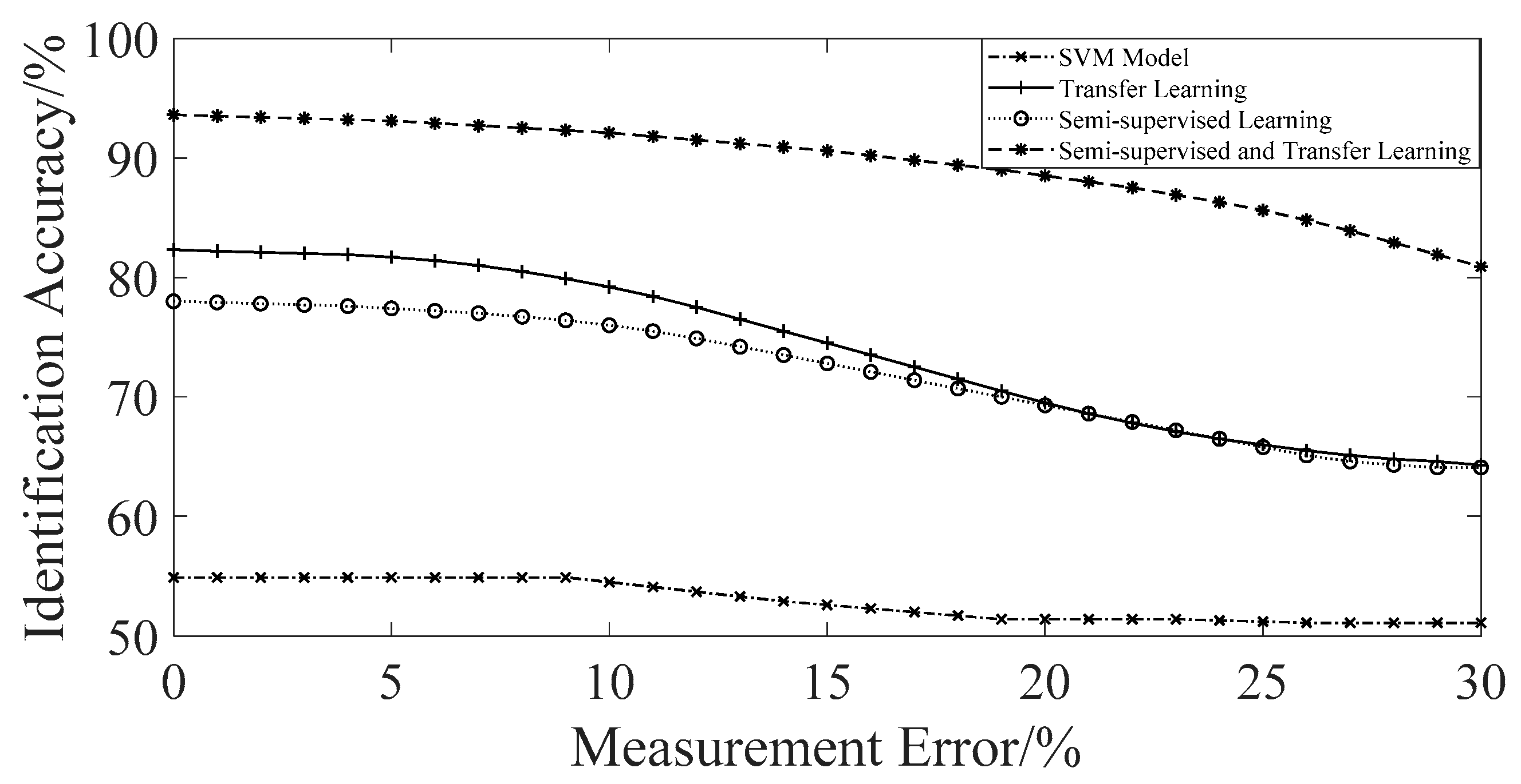
In order to further verify the effectiveness of the proposed method, we train the base classifier SVM model, the SVM model based on transfer learning, the SVM model based on semi-supervised learning and the SVM model based on semi-supervised and transfer learning respectively to identify the unknown radar emitter samples. In addition, in order to verify the adaptability of the model to the measurement error, we introduce an error deviation level test algorithm [21]. The specific experiment results are shown in Figure 5.

From the contrast experiment results, it can be known that when only using the base classifier SVM model for identification, the identification accuracy obtained is less than 55%. The main reason is that the known radar emitter data and the unknown radar emitter data do not satisfy the same-distribution hypothesis, resulting in an inability to obtain a valid classifier. When using the SVM model based on semi-supervised and transfer learning for identification, the optimal identification accuracy can be achieved within a certain measurement error range. Identification accuracy can reach more than 90% in the measurement error range of 15%, indicating that the method has good noise adaptability, and is obviously superior to the SVM model based on transfer learning, and the SVM model based on semi-supervised learning. The main reason is that the semi-supervised and transfer learning can make full use of sample information to achieve good performance without a lot of iteration.

The identification accuracy obtained by the SVM model based on transfer learning is slightly better than that obtained by the SVM model based on semi-supervised learning. The main reason is that there are not many available training samples in the target domain, which leads to the fact that only using the semi-supervised learning method cannot enhance the training effect. When the measurement error is greater than 10%, the identification accuracy of the transfer learning method and the semi-supervised learning method will be significantly reduced, indicating that their noise adaptability is not good.

4.4. Results Discussion

For the radar emitter identification task, deep learning models can often achieve the best results. Therefore, in this section, we construct the CNN model [6] and the U-CNN model [7] to compare with our method proposed in this paper. In the two deep learning models, radar pulse description words are used to represent radar signals, and as input to the model, which is the same as the processing of our method, so it is appropriate to compare CNN, U-CNN and our method together. The specific experiment results of different models are shown in

Table 3. Identification accuracy of different models.

Model	Identification Accuracy
	Traditional Scenario	Unknown Scenario
CNN	98.1%	72.2%
U-CNN	98.5%	76.3%
our method	95.3%	91.6%

. In the traditional identification scenario, that is, where we only use the labeled samples in source domain to train the models and then test on the source domain data, U-CNN can achieve the best performance. Its identification accuracy is up to 98.5%, while the identification accuracy of our method is only 95.3%. In the unknown identification scenario, that is, wherein we use the labeled samples in source domain and the unlabeled samples in target domain to train the models and then test on the unknown radar emitters in target domain, the identification accuracy of CNN and U-CNN decrease sharply. However, our method can still reach an identification accuracy of 91.6%. The experiment results show that compared with the currently most popular deep learning models, although our method still has disadvantages in the traditional identification scenario, it can achieve the best performance when facing unknown radar emitters.

5. Conclusions

In the radar emitter identification task, the traditional methods are often difficult to identify unknown radar emitters. Aiming at the problem, this paper proposes an unknown radar emitter identification method based on semi-supervised and transfer learning. The transfer learning method can solve the problem that the training data and testing data do not satisfy the same-distribution hypothesis, and the semi-supervised learning method can utilize the information of unlabeled samples to enhance the final training effect. Simulation experiments show that the proposed method can achieve an identification accuracy of 91.6% in the measurement error range of 15%, which is 15.3% higher than the deep learning model in the unknown identification scenario. The next step is to continue to optimize the model and lighten it for automatic compression, in order to minimize the running time of our method.

References

- Wiley, R.G. ELINT: The Interception and Analysis of Radar Signals, 1st ed.; Artech House: London, UK, 2006; p. 451. [Google Scholar]
- Jin, L.; Zhang, X.; Gong, J.Z.; Tang, J.T.; Ren, Z.Y.; Li, G.; Deng, Y.L.; Cai, J. Signal-Noise Identification of Magnetotelluric Signals Using Fractal-Entropy and Clustering Algorithm for Targeted DE-Noising. Fractals 2018, 26, 1840011. [Google Scholar]
- Li, J.C.; Ying, Y.L. Radar signal recognition algorithm based on entropy theory. In Proceedings of the 2014 2nd International Conference on Systems and Informatics (ICSAI), Shanghai, China, 15–17 November 2014. [Google Scholar]
- Yang, Z.T.; Qiu, W.; Sun, H.J.; Nallanathan, A. Robust Radar Emitter Recognition Based on the Three-Dimensional Distribution Feature and Transfer Learning. Sensors 2016, 16, 289. [Google Scholar] [CrossRef] [PubMed] [Green Version]
- Zhou, Z.W.; Huang, G.M.; Chen, H.Y.; Gao, J. Automatic Radar Waveform Recognition Based on Deep Convolutional Denoising Auto-Encoders. Circuits Syst. Signal Process 2018, 37, 4034–4048. [Google Scholar] [CrossRef]
- Cain, L.; Clark, J.; Pauls, E.; Ausdenmoore, B.; Clouse, R.; Josue, T. Convolutional neural networks for radar emitter classification. In Proceedings of the 2018 IEEE 8th Annual Computing and Communication Workshop and Conference (CCWC), Las Vegas, NV, USA, 8–10 January 2018; pp. 79–83. [Google Scholar]
- Sun, J.; Xu, G.L.; Ren, W.J.; Yan, Z.Y. Radar emitter classification based on unidimensional convolutional neural network. IET Radar Sonar Navig 2018, 12, 862–867. [Google Scholar] [CrossRef]
- Kong, M.X.; Zhang, J.; Liu, W.F.; Zhang, G.L. Radar Emitter Identification Based on Deep Convolutional Neural Network. In Proceedings of the 2018 International Conference on Control, Automation and Information Sciences (ICCAIS), Hangzhou, China, 24–27 October 2018; pp. 309–314. [Google Scholar]
- Wang, X.B.; Huang, G.M.; Zhou, Z.W.; Tian, W.; Yao, J.L.; Gao, J. Radar Emitter Recognition Based on the Energy Cumulant of Short Time Fourier Transform and Reinforced Deep Belief Network. Sensors 2018, 18, 3103. [Google Scholar] [CrossRef] [PubMed] [Green Version]
- Shi, Z.H.; Hao, H.; Zhao, M.H.; Feng, Y.N.; He, L.F.; Wang, Y.H.; Suzuki, K. A deep CNN based transfer learning method for false positive reduction. Multimed. Tools Appl. 2018, 78, 1–17. [Google Scholar] [CrossRef]
- Deng, H.; Ma, C.; Shen, L.J.; Yang, C.W. Semi-Supervised Learning Using Autodidactic Interpolation on Sparse Representation-Based Multiple One-Dimensional Embedding. Int. J. Wavelets Multiresolution Inf. Process. 2019, 17, 1950013. [Google Scholar] [CrossRef]
- Dainotti, A.; Pescape, A.; Claffy, K.C. Issues and future directions in traffic classification. IEEE Netw. 2012, 26, 35–40. [Google Scholar] [CrossRef] [Green Version]
- Zhu, Z.F.; Zhu, X.Q.; Guo, Y.F.; Xue, X.Y. Transfer incremental learning for pattern classification. In Proceedings of the 19th ACM Conference on Information and Knowledge Management (CIKM), Toronto, ON, Canada, 26–30 October 2010. [Google Scholar]
- He, Q.; Li, B.; Shen, B.; Xia, Y. Cross-Project Software Defect Prediction Using Feature-Based Transfer Learning. In Proceedings of the 7th Asia-Pacific Symposium, Wuhan, China, 6 November 2015. [Google Scholar]
- Montalto, A.; Marinazzo, D.; Kugiumtzis, D.; Nollo, J.; Faes, L. Comparing Model-Free and Model-Based Transfer Entropy Estimators in Cardiovascular Variability. In Proceedings of the Computing in Cardiology 2013, Zaragoza, Spain, 22–25 September 2013. [Google Scholar]
- Jefferson, T. Boosting Degree Completion and Transfer Rates: An Examination of Counseling/Advising Using the Relationship-Based Model. Online Submiss 2010, 36. Available online: https://eric.ed.gov/?id=ED538968 (accessed on 11 December 2019).
- Xu, X.P.; Zhu, X.W.; Liu, Q.Q. Can Self-Training in Mindfulness-Based Cognitive Therapy Alleviate Mild Depression Among Chinese Adolescents? Soc. Behav. Personal. Int. J. 2019, 47, 4. [Google Scholar] [CrossRef]
- Karamanolakis, G.; Hsu, D.; Gravano, L. Leveraging Just a Few Keywords for Fine-Grained Aspect Detection Through Weakly Supervised Co-Training. arXiv 2019, arXiv:1909.00415. [Google Scholar]
- Goodfellow, I.J.; Pouget-Abadie, J.; Mirza, M.; Xu, B.; Warde-Farley, D.; Ozair, S.; Courville, A.; Bengio, Y. Generative adversarial nets. In Proceedings of the Conference and Workshop on Neural Information Processing Systems, Montreal, QC, Canada, 8–13 December 2014; pp. 2672–2680. [Google Scholar]
- Kipf, T.N.; Welling, M. Semi-Supervised Classification with Graph Convolutional Networks. arXiv 2016, arXiv:1609.02907. [Google Scholar]
- Shieh, C.S.; Lin, C.T. A vector neural network for emitter identification. IEEE Trans. Antennas Propag. 2002, 50, 1120–1127. [Google Scholar]
Figure 1.
Specific process of the semi-supervised and transfer learning algorithm.
Figure 2.
Distribution and change characteristics of the five parameters of pulse amplitude (PA), carrier frequency (CF), pulse width (PW), pulse repetition interval (PRI) and angle of arrival (AOA).
Figure 3.
Impact of the semi-supervised learning method on the transfer learning method.
Figure 4.
Impact of the transfer learning method on the semi-supervised learning method.
Figure 5.
Contrast experiment results.