Planning the Schedule for the Disposal of the Spent Nuclear Fuel with Interactive Multiobjective Optimization


1
Department of Mathematics and Statistics, University of Turku, FI-20014 Turku, Finland
2
Laboratory of Mathematics, Tampere University of Technology, FI-28100 Pori, Finland
*
Author to whom correspondence should be addressed.
Algorithms 2019, 12(12), 252; https://doi.org/10.3390/a12120252
Submission received: 24 October 2019
/
Revised: 21 November 2019
/
Accepted: 22 November 2019
/
Published: 25 November 2019
(This article belongs to the Special Issue Nonsmooth Optimization in Honor of the 60th Birthday of Adil M. Bagirov)
Abstract
:Several countries utilize nuclear power and face the problem of what to do with the spent nuclear fuel. One possibility, which is under the scope in this paper, is to dispose of the fuel assemblies in the disposal facility. Before the assemblies can be disposed of, they must cool down their decay heat power in the interim storage. Next, they are loaded into canisters in the encapsulation facility, and finally, the canisters are placed in the disposal facility. In this paper, we model this process as a nonsmooth multiobjective mixed-integer nonlinear optimization problem with the minimization of nine objectives: the maximum number of assemblies in the storage, maximum storage time, average storage time, total number of canisters, end time of the encapsulation, operation time of the encapsulation facility, the lengths of disposal and central tunnels, and total costs. As a result, we obtain the disposal schedule i.e., amount of canisters disposed of periodically. We introduce the interactive multiobjective optimization method using the two-slope parameterized achievement scalarizing functions which enables us to obtain systematically several different Pareto optimal solutions from the same preference information. Finally, a case study adapting the disposal in Finland is given. The results obtained are analyzed in terms of the objective values and disposal schedules.
1. Introduction
The disposal of the spent nuclear fuel is a challenging task where the careful planning and optimization of processes definitely pays dividends. The difficulty of the decision making is increased also by the fact that the disposal continues for the distant future and many parameters are still unknown. Indeed, the decisions made now have long term consequences. Thus, it is only reasonable to investigate different scenarios by utilizing multiobjective optimization from the different perspectives.
The disposal is a topical issue since many of the countries utilizing nuclear power have not yet disposed of any spent nuclear fuel. Nevertheless, all of them have to do something for it sooner or later. Long-term storage in interim storage is not considered a safe or ethical solution [1]. At the same time, the geological disposal is stated to be widely accepted as a safe method [1]. Finland is going to be one of the first countries to dispose of the spent nuclear fuel by starting the disposal in 2020s [2].
The aim in the geological disposal is to isolate the spent nuclear fuel to the bedrock such that it has no more impacts on the environment than the regular background radiation. First, the fuel assemblies are removed from the reactor and stored in the water pool in the reactor hall in order to decrease the radiation and the decay heat power to the suitable level such that the assemblies can be transferred to the water pool in the interim storage facility for decades. When the assemblies are cool enough, they can be transferred to the encapsulation facility, where the assemblies are encapsulated into the copper-iron canisters. After that, the canister moves on towards the disposal facility, in depth of more than 400 m. The disposal facility consists of the central tunnel and several parallel disposal tunnels that are connected to the central tunnel. The canister is placed vertically in the hole on the floor of the disposal tunnel. Finally, the disposal tunnel is filled up and sealed. In this study, we divide the disposal process into three parts: the interim storage, the encapsulation facility, and the disposal facility.
As the entire nuclear waste management is a large task, optimization related studies about it are usually focused on some smaller entities. Some of these entities are concentrated more on political or social aspects like to determine where to put a disposal repository [3] or how to route the transfer of the nuclear waste, or hazardous waste in general [4,5]. More safety-related aspects are the optimization of the nuclear safeguards [6,7] and the safety assessment of nuclear waste repositories [8]. In our study, we aim to produce a disposal schedule such that several goals related to all the interim storage, the encapsulation facility, and the disposal facility are taken into account simultaneously with multiobjective optimization. Other studies aiming at a disposal schedule are, for example, [9] where a single-objective mixed-integer linear programming (MILP) model minimizing the costs is given and [10] trying to achieve the minimal area of the disposal facility with a linear transportation model. Another research related to the disposal facility is discussed in [11], where the multiobjective MILP problem is given to optimize the nuclear waste placement in the disposal facility. In addition, there are attempts to optimize the loading of canisters in Finland [9,12], Slovenia [13], and Switzerland [14].
This study continues the work of [9], where the aim was to minimize the total costs of the disposal in Finland by selecting the schedule of the disposal. Here, this work has been continued by remodeling the situation as the nonsmooth multiobjective mixed-integer nonlinear programming (MINLP) problem. As a nonsmooth optimization problem [15,16,17], the objectives and the constraints are not necessarily continuously differentiable functions. This allows us to model the situation more accurately. Indeed, many practical applications have nonsmooth nature (see e.g., [18,19,20]) even if they are modeled as differentiable problems in many cases in practice.
Many practical problems also involve several objectives [21,22,23,24]. As a problem of this scale, this application has several conflicting objectives to offer naturally. Besides total costs, it is reasonable to optimize, for instance, the area of the disposal facility. In our model, this is done by minimizing the lengths of both disposal and central tunnels. In total, our model contains nine objectives. In addition to the previous three objectives, we have three objectives related to the interim storage and three related to the encapsulation facility. In the interim storage, we want to minimize the maximum number of assemblies in the storage, the maximum storage time, and the average storage time. On the other hand, the operation time of the encapsulation facility is aimed to be minimized and al number of canisters, or in other words, the number of the empty assembly positions.
These objectives indeed are conflicting. For instance, we want the whole disposal process to be over as early as possible, but this raises the heat production load of the canister. This in its turn, increases the distances between the canisters in the disposal facility. However, the heat load of the canister can be decreased by leaving empty assembly positions, but then more canisters are needed. Another option is to increase the cooling time which again delays the end of the disposal, but if the disposal delays, more storage space is needed. Obviously, all of these decisions have an impact on costs. As exemplified, the minimization of only one objective may lead to an unsatisfactory solution with respect to some other objective. This leads us to a situation where compromises are certainly needed.
As a result of the multiobjective optimization, we obtain several mathematically equally good compromises, called Pareto optimal solutions. The final selection is left to the decision-maker who has more insight into the problem. In this paper, we propose an interactive procedure utilizing the achievement scalarizing function (ASF), in particular, the two-slope parameterized ASF [25] which bases on parameterized ASF [26] and two-slope ASF [27] generalizing both of them by combining their advantages. Via scalarization, the original multiobjective problem is transformed into one single-objective problem. The idea in brief with ASF is that the decision-maker gives a reference point including the decision maker’s wishes towards the final solution. Then, the closest optimal solution with respect to some metric is found. If we use only one metric, as is the case in general with ASF, the selected metric defines which solution is found [28,29,30]. With the parameterization, we are able to use several metrics, nine in this particular case, and thus, yield different solutions with reasonable distribution. This ability to systematically generate different solutions from the same preference information is utilized in the interactive framework.
This paper is organized as follows. In Section 2, we begin by depicting the situation under the consideration and give a nonsmooth multiobjective MINLP model for it. In Section 3, we first introduce some fundamental preliminaries about multiobjective optimization, and then describe the multiobjective interactive method utilizing two-slope parameterized ASFs (MITSPA). In Section 4, one special case study of the disposal in Finland is given and the solutions are analyzed. Finally, in Section 5 some concluding remarks are discussed.
2. Mathematical Model
In this section, we give a comprehensive description of the model for scheduling the disposal of the spent nuclear fuel. The aim is to provide general guidelines for the disposal schedule and we only plan how many canisters are disposed of rather than which assemblies are placed in which canister nor give any complex lay-out for the disposal facility. We model the situation adapting the disposal in Finland as described in the introduction with some limitations like we omit the transportation between the facilities. Furthermore, we suppose that nothing is disposed of yet and only one type of fuel is considered. Some other simplifying assumptions are that we have access to all the assemblies, assemblies are identical, and the bedrock is homogeneous such that we can build tunnels anywhere.
The model formulated is a nonsmooth multiobjective MINLP problem having nine objectives. One obvious objective is total costs. Due to the long term time perspective of the disposal, the costs will probably change during the years so we minimize also some cost factors as their own objectives. Besides being a cost factor, these objectives have also other reasons to be selected as an objective. The interim storage-related objectives minimize storage times and amounts. The faster the assemblies get under the ground, the safer it is. Other safety issues are handled as constraints, like the cooling time of the assembly must be sufficient, the maximum decay heat power of the canister is limited, and the distances between disposal tunnels and canisters depend on the heat load of the canister. While we allow empty positions in canisters, we still try to keep the total amount of the canisters as low as possible. The other objectives related to the encapsulation facility aim to get disposal done as soon as possible. Finally, the area of the disposal facility is minimized.
2.1. Parameters
The model involves several parameters mostly dealing with lower and upper bounds and costs. First, we begin with two parameters determining the size of the model. Let
| N | be a total number of disposal periods |
| Z | be a total number of removals from the reactor. |
In addition, we define two sets of indices: the set of periods and the set of removals from the reactor . Note that part of the removals are done before the first disposal period begins. In order to link the removals from the reactor and periods, we introduce two parameters:
| a | the last removal before the first disposal period |
| b | the disposal period when the last removal is done. |
In the following, we specify notation and measurement units for some physical magnitudes:
| number of assemblies belonging to the removal | |
| Q | length of one disposal tunnel [m] |
| storage time of an assembly belonging to the removal | |
| in the period [period] | |
| decay heat power of an assembly belonging to the removal | |
| in the period [W]. |
The next seven parameters describe the cost information needed as an input data for the model:
| storage cost per one assembly per period [€] | |
| costs related to the interim storage per period [€] | |
| cost of a storage place per one assembly [€] | |
| cost of one canister [€] | |
| costs related to operating the encapsulation facility per period [€] | |
| cost of a disposal tunnel per meter [€] | |
| cost of a central tunnel per meter [€]. |
Finally, we give some parameters related to the upper and lower bounds:
| R | minimum storage time of an assembly [period] |
| K | maximum capacity of a canister |
| T | minimum number of canisters disposed in one period |
| U | maximum number of canisters disposed in one period |
| , | lower and upper bound for the maximum average power of |
| a canister [W] | |
| , | lower and upper bound for the distance between canisters [m] |
| lower and upper bound for the distance between disposal | |
| tunnels [m]. |
2.2. Continuous Variables
The model involves continuous variables such that they all are assumed to be non-negative. The continuous variables used are:
| number of assemblies belonging to the removal disposed during | |
| the period | |
| number of canisters disposed during the period | |
| number of assemblies belonging to the removal being in storage | |
| at the end of the period | |
| maximum average power of a canister | |
| distance between two adjacent disposal tunnels | |
| distance between two adjacent canisters in a disposal tunnel. |
Note that the first three variables have integer nature, but in order to ease the computation, they are relaxed as continuous variables.
2.3. Binary Variables
Besides continuous variables, the model consists also binary variables listed below:
| encapsulation starts in the beginning of the period | |
| encapsulation ends in the beginning of the period | |
| encapsulation facility is in operation during the period | |
| assemblies belonging to the removal take off from disposal | |
| at the beginning of the period | |
| indicates that assemblies belonging to the removal | |
| can be disposed during the period . |
2.4. Objectives
The model involves nine objectives such that six of them are nonlinear and three are linear. These objectives are:
Note that from nonlinear objectives, the objectives (1), (2), (5) and (9) are also nonsmooth. The objectives (1)–(3) are related to the interim storage such that (1) minimizes the maximum number of assemblies in the storage, (2) minimizes the maximum storage time, and (3) minimizes the average storage time. In the objective (1), with the first component we take into account the first a removals from the reactor where all the assemblies must be stored simultaneously. The second component handles the cases when removals are accomplished during the disposal periods. Finally, with the third component the cases when all removals are done are considered.
The next three objectives (4)–(6) are related to the encapsulation facility. The objective (4) minimizes the total number of canisters, (5) aims to stop the disposal as early as possible, and (6) minimizes the time which the encapsulation facility is in operation.
The objectives (7) and (8) aim to minimize the size of the disposal facility such that (7) minimizes the total length of disposal tunnels and (8) minimizes the length of the central tunnel.
Finally, the ninth objective (9) minimizes the total costs of the disposal process. The costs taken into account are related to the storage, cost of individual canisters, the encapsulation facility operating costs, and the building costs of the disposal and central tunnels.
2.5. Constraints—Interim Storage
The first set of constraints are related to the interim storage. All of these constraints are linear.
The constraints (10)–(12) define the variables depicting the amount of assemblies in storage. The constraint (13) enforces all the assemblies to be disposed once. With the constraints (14)–(16) the variables are defined. The constraint (17) ensures that the production capacity is not exceeded and the constraint (18) ensures that the assembly disposed has been cooling long enough.
2.6. Constraints—Encapsulation Facility
In order to guarantee the acceptable encapsulation, the following linear constraints are needed.
The constraints (19) and (20) ensures that the encapsulation facility is switched on and off exactly once meaning that all the canisters must be encapsulated at once. The constraints (21) and (22) define the variable . The constraints (23)–(25) guide the encapsulation process: (23) guarantees that there exist enough canisters such that all the assemblies can be disposed, (24) keeps the number of canisters under the production capacity, and (25) forces the minimum production to be fulfilled.
2.7. Constraints—Disposal Facility
The number of constraints related to the disposal facility is such that of them are nonlinear, and three of the constraints are box constraints.
The constraints (26) and (27) are the nonlinear constraints of this model. The constraint (26) ensures that the heat power of the canisters disposed is allowable while the constraint (27) defines the dependence between the variables , , and . In our case, this nonlinear function is approximated with a piece-wise linear function (see Appendix A). Finally, the box constraints (28)–(30) give lower and upper bounds for variables , , and , respectively.
Finally, we give some boundaries for the variables:
To conclude, the model has nine objectives such that 6 are nonlinear and 3 are linear. The rest of the dimensions of the model are depending on two parameters: the number of periods N and the number of the removals from the reactor Z. Number of constraints is , where are linear, nonlinear and 3 box constraints. The total number of variables is and of them are non-negative continuous variables and are binary variables. Evidently, with any realistic values of N and Z, for example and when one period is five years, the size of the problem will come quite large.
3. Multiobjective Optimization Approach
In this section, we define some fundamental aspects on multiobjective optimization, and then, describe the family of two-slope parameterized achievement scalarizing functions (ASFs) [25] with its properties. Finally, the interactive method utilizing two-slope parameterized ASFs is introduced.
3.1. Mathematical Background
We consider the following multiobjective MINLP problem of the form
where is a decision variable, C is the set of constraints, and X is a nonempty and compact set of feasible solutions. The objectives for all are assumed to be lower semicontinuous with respect to and at least partially conflicting. Therefore, we cannot find a minimal solution for every objective simultaneously and the minimization of only one objective may lead to an arbitrary bad solution with respect to other objectives. In order to compare the objectives, for we denote by if for all and if for all .
In multiobjective optimization, we say that a solution is Pareto optimal if we cannot improve any objective without causing a deterioration for some other objective at the same time. Mathematically speaking, a solution is Pareto optimal if there does not exist any solution such that and for at least one index . It is noteworthy that usually we do not have a unique Pareto optimum but a set of Pareto optimal solutions, called the Pareto set. All these Pareto optimal solutions belong also to a larger class of weakly Pareto optimal solutions. The solution is an element of this class if there does not exist another solution such that .
In order to obtain some information about the Pareto set, we can define an ideal and a nadir vector, and , to give the lower and the upper bound for a Pareto optimal solution, respectively. The ideal vector consists of individual minima of the objectives. This means that the component is calculated as a solution of the problem . Due to the conflicting objectives, the ideal vector is not feasible. The nadir vector, in its turn, represents the worst objective values in the Pareto set. Unfortunately, the exact calculation of the nadir vector needs the maximization of objectives over the set of Pareto optimal solutions being a hard task. Thus, the nadir vector needs to be approximated, for example, with a pay-off table (see e.g., [31,32]).
3.2. Two-Slope Parameterized ASFs
We approach the multiobjective mixed-integer problem with a special type of achievement scalarizing functions. In general, the utilization of the achievement scalarizing function (ASF) aims to find a Pareto optimal solution being as close as possible to a so-called reference point . The components , include the decision maker’s wishes for each objective. This search is done by transforming the multiobjective optimization problem to a certain type of a scalarized problem and then applying some suitable single-objective optimization method.
We use here the two-slope parameterized ASF, proposed in [25], which is a generalization of the parameterized ASF [26] and the two-slope ASF [27]. Usually, to find the closest point to the reference point , the distance from is measured with only one metric. With the parameterization used in the parameterized ASF and the two-slope parameterized ASF, we can combine different metrics such that and metrics are the extreme cases. Thus, by systematically producing different Pareto optimal solutions from the same preference information, we can give the decision maker a wider perspective to the range of Pareto optimal solutions. Another benefit of the two-slope parameterized ASF, as well as the two-slope ASF, is that we do not need to test the achievability of the reference point. This is due to the fact that the different weights are used depending on if the reference point is achievable (i.e., the reference point belongs to the image of the feasible solutions in the objective space) or unachievable. The use of different weights is reasonable since the decision-maker usually prefers different solutions if the reference point is achievable or not, as was suggested in [28].
In order to solve the model described in Section 2, we apply the two-slope parameterized ASF. Once the multiobjective problem is converted to the single-objective one, we obtain a scalarized version of the problem (31) in the form [25]
where the weighting vectors for all are for the unachievable and the achievable reference point, respectively. The parameter specifies which metric is used and is a set containing q integers from the interval , where k is the total number of objectives. Then, the maximization is taken over all the sets including q integers from the interval . In order to gain the benefits of the parameterization, or in other words, to use more metrics than only (i.e., ) and (i.e., ), the problem must contain at least three objectives while the maximum number of different metrics equals the number of the objectives.
Next, we are interested to know what can be deduced from the optimal solution of the scalarized problem. As the justification for the use of the two-slope parameterized ASF, we can proof the following results by adapting the proofs from [25].
Theorem 1
Proof.
(i) Assume that is an optimal solution of the problem (32) but not a weakly Pareto optimal solution of the problem (31). Then there exists a feasible solution such that . For any , denote , and as the objective of the scalarized problem (32). Now
yielding to a contradiction.
(ii) Assume that is an optimal solution of the problem (32) but not a Pareto optimal solution of the problem (31). Therefore, there exists such that and at least one index such that . Similarly to (i), we can deduce that . If the equality holds, is an optimal solution for the problem (32) and Pareto optimal for the problem (31). In the case of strict inequality, this yields to a contradiction with an assumption that is an optimal solution for the problem (32).
(iii) First, we observe that is strictly increasing (i.e., for any having and ). Indeed, by taking such that , we see that
Thus, we know that every Pareto optimal solution can be obtained and the solution of the scalarized problem (32) is weakly Pareto optimal for the original multiobjective problem. In order to guarantee the Pareto optimality of solutions, a so-called augmentation term [32]
may be added to the objective of the scalarized problem (32) [25]. Note that similarly to Theorem 8 in [25] it can be proven that if the set X and the objectives , are convex, then preserves the convexity.
3.3. Multiobjective Interactive Method Utilizing the Two-Slope Parameterized ASFs
In the following, we state an outline of the multiobjective interactive solution approach utilizing the two-slope parameterized ASFs (MITSPA) applying reference point based preference information. The general framework of interactive methods is usually similar: firstly, some range for Pareto optimal solutions is given the decision-maker, secondly, the decision-maker provides some preference information, thirdly, some solutions are presented for the decision-maker, and fourthly, the decision-maker express his/her opinion on the solutions and modify the preference information as a base for the new solutions. The process is stopped when the decision-maker is satisfied with the solution. The main differences in various interactive methods can be found in the ways the preference information is given and which solvers are applied (see e.g., [32,33]).
Similar approaches to ours in terms of the utilization of scalarization functions and the reference point as preference information are proposed, for instance, in [32,33,34,35,36,37,38]. Compared with these, in our case with the two-slope parameterized ASFs, we can systematically produce different Pareto optimal solutions to obtain a reasonably distributed selection of Pareto set.
Multiobjective interactive method utilizing the two-slope parameterized ASFs (MITSPA)
- Step 0.
- Give the ideal vector , the nadir vector , and/or some Pareto optimal solution to the decision maker in order to illustrate the Pareto set.
- Step 1.
- Set the iteration counter and select the maximum number of iterations . Ask the decision maker to provide the reference point and the number of solutions presented for each reference point. Initialize the positive coefficients and .
- Step 2.
- Step 3.
- Present s solutions to the decision maker and ask the decision maker to select the most preferable solution among them as the current solution and go to Step 5 or if more solutions for the current reference point are needed go to Step 4.
- Step 4.
- Present supplementary solutions to the decision maker. Ask the decision maker to select the most preferable solution among the previous s solutions and the supplementary solutions as the current solution and go to Step 5.
- Step 5.
- If or the decision maker is satisfied with the current solution , stop with the current solution as the final solution . Otherwise, ask the decision maker to specify the new reference point as the current reference point, set , and go to Step 2.
Some remarks about the above algorithm are in order. Step 0 consists of the illustration of the Pareto set. Some Pareto optimal solutions for the decision-maker to start with can be calculated, for example, by using the two-slope parameterized ASF (32) with an ideal vector as a reference point or by applying some suitable no-preference method like descent methods [39,40,41,42,43]. In Step 3, solutions are presented to the decision-maker, where the k is the number of objectives. As mentioned, with the two-slope parameterized ASF we are able to solve as many different solutions as there are objectives. If the number of objectives is high, it facilitates the task of the decision-maker if only some of these solutions are presented. However, if the decision-maker is willing to see more solutions from the same reference point, this is enabled in step 4. If more than k solutions are needed in total for one reference point, they can be obtained by varying the coefficients and . During the solution process, the decision maker is able to learn about the model and after seeing some solutions, the decision maker has more insight into the problem and might want to change the opinion on the good reference point. Thus, in Step 5, a new reference point is allowed and new solutions are solved in Step 2.
4. Case Study: The Disposal in Finland
In practice, the scalarized problem (32) with an augmentation term (33) in Step 2 of MITSPA is solved with a branch-and-cut type method for single-objective MINLP problems called BARON [44,45] in GAMS [46]. The CPU time of solving each problem (32) presented here varies from 9 s to 28000 s while the average CPU time is 3475 s and the median CPU time is 142 s. The weighting vectors used are of the form
such that and as suggested in [27]. The approximation of the nadir vector used is obtained with a pay-off table [31,32].
We investigate the disposal of the spent nuclear fuel from the European pressurized water reactor (EPR) produced by Olkiluoto 3 in Finland starting to operate in the near future. The length of one disposal period is selected to be 5 years, and the parameters N and Z are 19 and 11, respectively. The other parameters used are given in Appendix A, except the cost parameters that are omitted due to their commerce-related nature. This parameter selection yields a multiobjective MINLP problem with 9 objectives, 440 continuous and 475 binary variables, 1144 linear constraints, 20 nonlinear constraints, and three box constraints. Apart from these, we need some auxiliary variables and constraints to overcome the non-smoothness of the problem. Indeed, the two-slope parameterized ASFs are nonsmooth, but due to their min-max structure, the problem (32) can be written in the MINLP form as in [25]. Similarly, this trick can be applied also for the nonsmooth objectives. After that, we have to solve a single-objective problem with 441 continuous and 484 binary variables, 1153 linear constraints, 21–146 nonlinear constraints and 3 box constraints.
Before we proceed to the solution process, we discuss the trade-offs of the problem. There are three parts in the final disposal of spent nuclear fuel: the interim storage, the encapsulation facility, and the disposal facility. These three parts interact with each other as is exemplified in the following.
- Interim storage versus disposal facility: The interim storage-related goals all imply transferring the spent nuclear fuel from the interim storage as rapidly as possible. However, in order to minimize the disposal facility-related goals, the cooling times should be maximized.
- Encapsulation facility versus interim storage: By delaying the start of disposal, it is possible to shorten the operation time of the encapsulation facility, and thus, decrease the operating costs. Again, the delay at the start of the encapsulation can cause an increase of the inventories in the interim storage.
- Encapsulation facility versus disposal facility: The disposal should be started and ended as soon as possible. Both of these aims have a tendency to increase the canister heat load, and hence, affect the disposal facility goals. To minimize the operation time of the encapsulation facility, empty assembly positions can be used. However, the price to pay is the increased number of canisters. In addition, a larger number of canisters necessitates an increase in the disposal facility area.
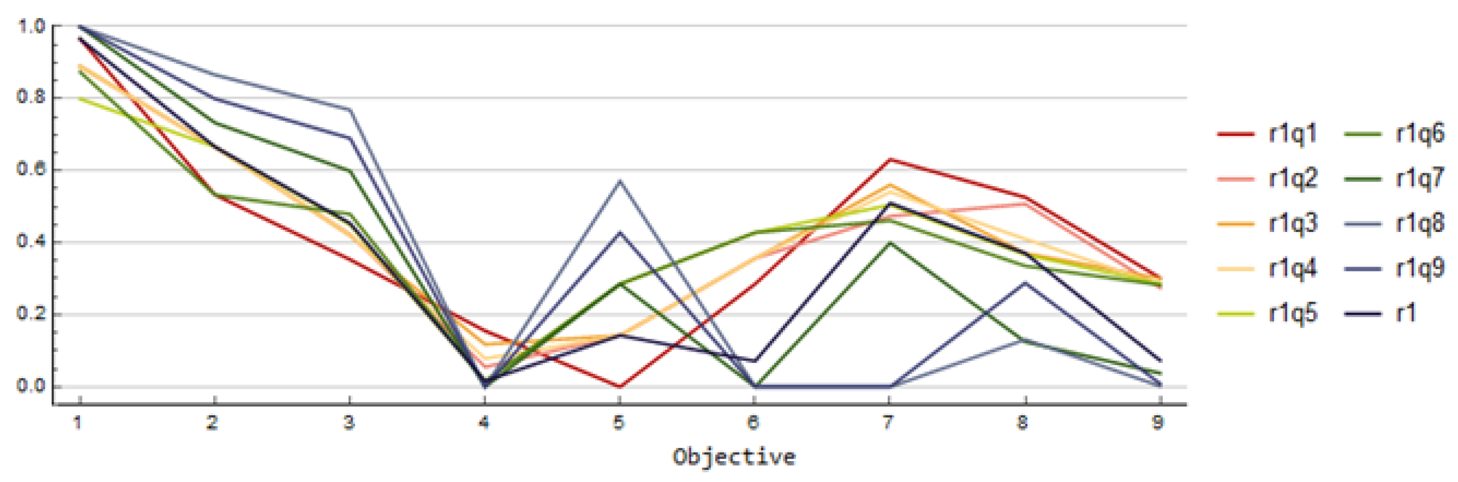
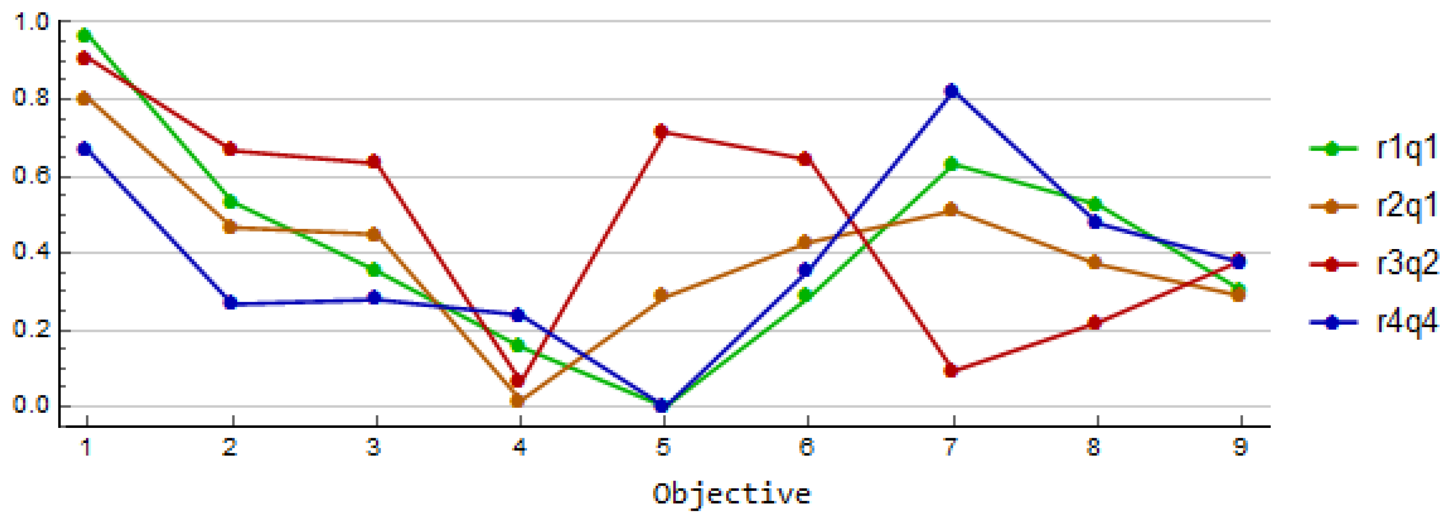
In order to investigate these, and other trade-offs, the interactive method MITSPA is employed. In each iteration of MITSPA, some new preference information is asked from the decision-maker reflecting his/her preferences. For each iteration, we compute nine solutions by using the current reference point with different metrics by varying the value of the parameter q from 1 to 9 in Step 2. In order to exemplify this, the nine solutions computed using reference point 1 are shown in Figure 1. These nine solutions represent different trade-offs between objective function values. The results obtained are scaled to the interval from 0 to 1 such that 0 is the value of the ideal vector and 1 is the value of the nadir vector for the objective under consideration. The different solutions are labeled based on the reference point used and the value of the parameter q. For example, the solution r1q1 is the result obtained by using the reference point 1 and . Moreover, the reference point 1 is labeled with r1.
In Step 3, two solutions are selected to be presented for the decision-maker for the closer inspection. The number of presented solutions s is restricted to two in order to aid the decision maker’s task to select best out of only two options and in order to keep the presentation clear. At each iteration, one solution with a smaller value of q and one with a larger value of q are presented and different values of q are demonstrated in order to exemplify the variety of solutions. Next, we present four iterations of MITSPA.
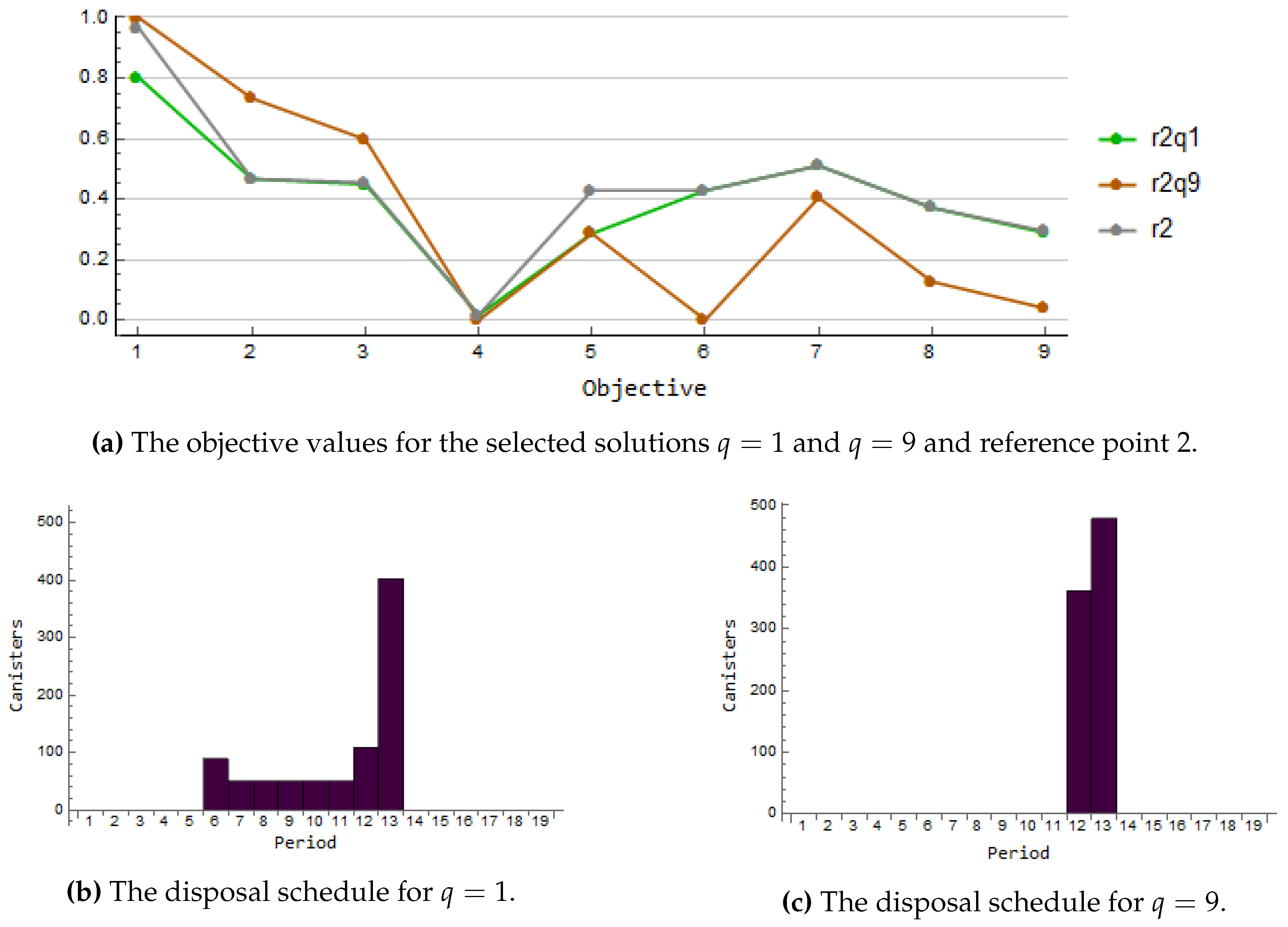
Iteration 1. At the first iteration, the decision maker begins by investigating the trade-off between operation time of the encapsulation facility and the cooling times of assemblies by deciding to start with the unachievable reference point such that the operation time is short and the cooling time is long. The two solutions chosen for reference point 1 are shown in Figure 2a together with reference point 1. The solution obtained by using value (r1q1) shown in the green line corresponds to the early starting time of disposal. The solution obtained by using value (r1q9) shown in the orange line corresponds to the late starting time of the disposal. In Figure 2b,c, the corresponding disposal schedules are given. The solution r1q9, has the shortest possible encapsulation time but the maximum cooling time is long. The solution r1q9, like r1q1, has a high maximum number of assemblies in the storage (see the objective (1)), but the maximum and average storage times (the objectives (2) and (3)) are slightly shorter. The solution r1q9 does not allow any empty positions in canisters while the solution r1q1 does (see (4)), but the encapsulation ends much later (see (5)) in the solution r1q9 than in r1q1. However, the operation time of the encapsulation facility (see (6)) is shorter in the solution r1q9 than in r1q1. When the disposal facility-related objectives (see (7) and (8)) are compared, the solution r1q9 needs a smaller area than the solution r1q1. Moreover, the solution r1q9 is cheaper than the reference, while the solution r1q1 is more expensive than the reference (see (9)). Mainly due to the significant difference in the costs, the decision maker selects the solution r1q9 as the current solution .
Iteration 2. In order to learn more about the trade-off between the operation time of the encapsulation facility and the cooling time, another reference point (reference point 2) is selected. In this case, the reference point is achievable. Now we try to find solutions such that the operation time is longer and cooling time shorter. The two solutions chosen for reference point 2 are shown in Figure 3a and the corresponding disposal schedules in Figure 3b,c. Again, the solution obtained with the small value (r2q1) represents the early starting time of the disposal. This is depicted with the green line in Figure 3a while the orange line depicts the solution obtained using value (r2q9) corresponding to the late starting time of the disposal.
If we compare the disposal schedules in Figure 3b,c to the schedules for reference point 1 given in Figure 2b,c, we notice some similarity. Even though the starting and ending times differ as well as the total number of canisters, the solutions with the parameter q value 1 and value 9 have the same shape. The smaller q suggests the schedule such that first, we encapsulate a small number of canisters per period and the number of canisters is growing while the time goes by, whereas the larger q recommends the schedule where all the canisters are encapsulated within two periods. The solution r2q1 captures the reference point well since they coincide with respect to other objectives than the objectives (1) and (5) which are better than the reference values. Thus, the decision maker is willing to continue with the solution r2q1 as the current solution .
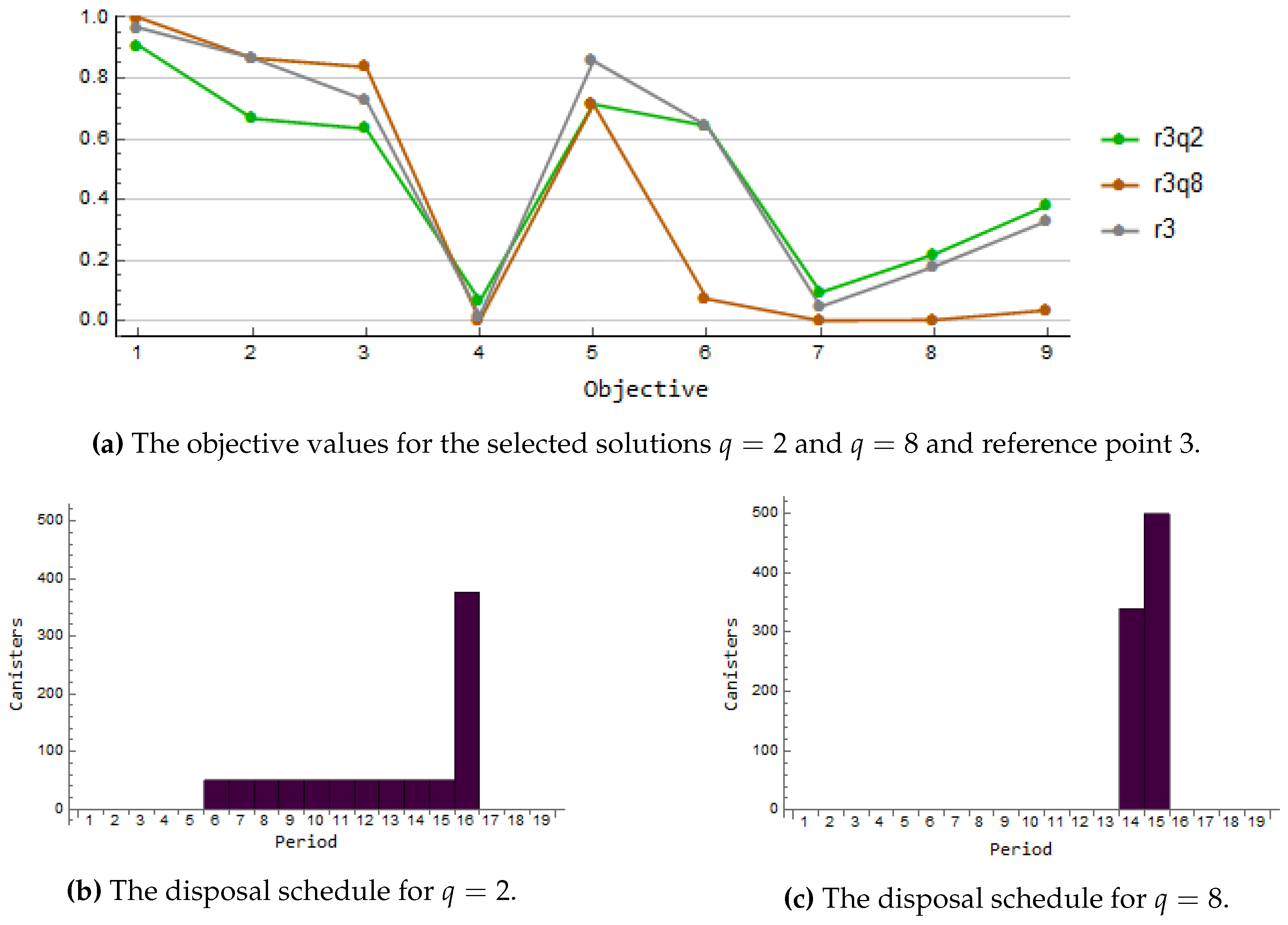
Iteration 3. The long operation time of the encapsulation facility (the objective (6)) is still under the microscope at the third iteration but the decision-maker is tempted by the short central tunnel appeared in the previous iteration and combines the long operation time with small disposal facility area. Like the first reference point, also this is unachievable. The solution obtained by using (r3q2) is shown in green and the solution obtained with (r3q8) is shown in orange in Figure 4a. Figure 4b illustrates that the solution r3q2 yields a schedule with an early starting date and the disposal takes the longest time while the solution r3q8 starts the disposal later but it is performed faster as seen in Figure 4c. The solution r3q8 yields almost ideal value for the costs, and we can deduce that in order to achieve lower costs we have to give up in the objectives related to the storage capacity and times. Moreover, the disposal ends rather late. For the current solution the decision-maker selects the solution r3q8 due to the low costs and small disposal facility area.
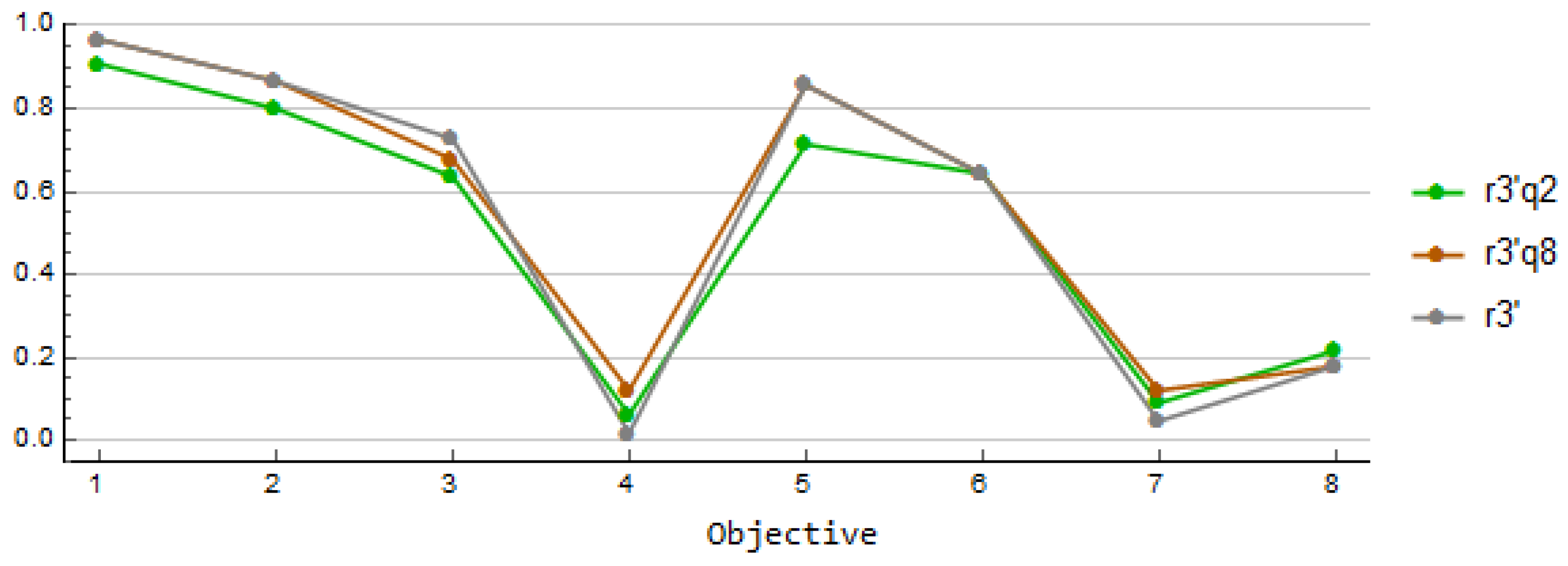
Since one motivation for this research was to take into account more goals than just the costs, we are eager to see what happens if we omit the costs and solve the problem with only the first eight objectives (1)–(8). The reference point 3’ is similar to the reference point 3 without the value for the costs. The results with (r3’q2) and (r3’q8) are given in Figure 5. Note that since there are now only eight objectives, the scalarized function is different than in the case of nine objectives. The solutions in Figure 5 are quite similar and there is less variation than in the solutions in Figure 4a.
Iteration 4. The current solution has high interim storage capacity and a small amount of canisters. At the fourth iteration, the decision maker is interested in to see if the opposite is possible, namely a solution with small interim storage capacity with allowing the higher number of canisters. Again, the reference point is unachievable. In Figure 6a, the reference point 4 and the solutions with (r4q4) and (r4q9) are illustrated. The solutions are shown in green and orange, respectively. Again, the corresponding disposal schedules are given in Figure 6b,c. As we see, the solution r4q4 satisfies the wishes towards the interim storage capacity as well as the utilization of the empty canister positions quite well. Additionally, the better values than the reference are obtained in the repository area related goals and the costs. The solution r4q9 express this as well, but the original wishes towards the interim storage capacity are not satisfied. Since the solution r4q4 captures better the ideas of the decision-maker, it is selected for the current solution .
Eventually, the decision maker is ready to make the final choice. During the solution process, we have learned that the solutions obtained from 4 different reference points can be split broadly into two main groups. The first group includes solutions where the disposal starts early while the other group includes the solutions with late starting. The most striking fact is that the solutions of the first group are obtained with smaller values of q and the solutions of the second group with the larger values of q. This phenomenon is repeated with all of four reference points. Interestingly, with the modified reference point 3 where only eight objectives were considered, mainly solutions with earlier starting time were obtained. In general, the earlier starting time of the disposal improves the objectives (1)–(3) and impairs others compared with the case where the disposal starts later. In general, we notice that the solutions obtained adapt the reference points quite well.
In Figure 7, the solutions related to the first group with an early starting time are illustrated. It can be seen that even if all these solutions suggest the early start of the disposal, they still have some differences. One can improve goals (7) and (8) by disposing of spent fuel with a small volume at the beginning. However, this declines goals (1)–(3), (5), (6) and (9) which can be seen from the solution r3q2. It is possible to improve the goals (1)–(3), (5) and (6) by allowing some canister positions to be empty. However, this in its turn declines goals (4) and (7)–(9) which can be seen from the solution r4q4. As the final solution, the decision maker likes to return to the reference point 2 and the solution r2q1 looks like a good compromise when disposal begins early.
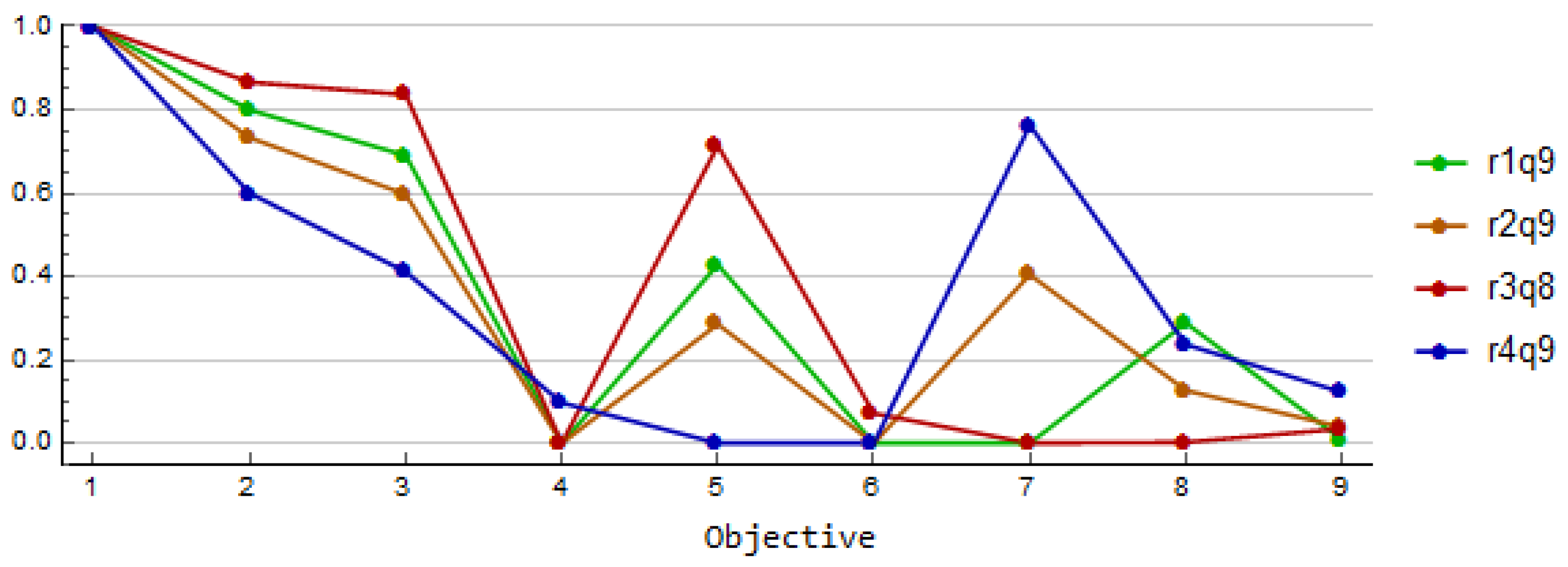
A similar examination is done for the solutions of the second group with the late starting time. The solutions in terms of the objective function values and the disposal schedules are given in Figure 8. Again, we can observe some differences. The differences depend on the number of years the start of disposal operations is prolonged. It can be seen from Figure 8, that the disposal volume is large in every solution where disposal starts late. On the one hand, one can improve goals (7)–(9) by delaying the start of disposal but on the other hand, this declines goals (2), (3) and (5), as illustrated in the solution r3q8. When the disposal starts late, empty canister positions have only a minor impact on the solution. One can improve goals (2), (3), and (5) by allowing empty canister positions. This yields to the impairing of the goals (4), and (7)–(9) which can be seen from the solution r4q9. Again, the decision maker is willing to return to the reference point 2 and consider the solution r2q9 as a satisfactory solution when the disposal starts late. Additionally, the decision maker selects this solution also for the final solution , since it yields a rather good solution for other objectives than the maximum storage. However, we learned that this is the price of the lower costs and smaller disposal facility area. Moreover, compared with the solution r2q1 also presented from the reference point 2, the later starting does not delay the ending of the disposal.
5. Conclusions
In this paper, we have proposed the nonsmooth multiobjective MINLP model to optimize the spent nuclear fuel disposal in order to obtain a disposal schedule. The modeled process is described and the model is presented in detail. Then, the two-slope parameterized ASF is briefly stated and validated the use of it. Additionally, we proposed an interactive solution method utilizing these ASFs. Finally, some numerical results from the case study are given. The solutions obtained are exemplified and analyzed in terms of objective function values and disposal schedules.
With slight modifications, the model presented is applicable to other countries than Finland as well, if the spent nuclear fuel is decided to dispose of the disposal facility. It is possible to change the objectives or leave some of them out. Indeed, this model has quite many objectives, and in some cases it may be advantageous to have fewer goals either to ease the decision maker’s task or reduce the computations needed.
The schedules obtained are realistic and viable. One conspicuous feature for the solutions is that they are segmented in two groups based on the value of the parameter q enabling the parameterization when the two-slope parameterized ASF is used. With the lower values of q (i.e., closer to metric), the disposal starts early and with the larger values of q (i.e., closer to metric) the later start of the disposal is suggested. If only one metric, for instance metric, was used, no solutions with late starting would have been obtained in these iterations. For further studies, it would be interesting to investigate, is this kind of phenomenon observable in other applications as well, if the two-slope parameterized ASF is used. The role of q is also fascinating in terms of which value of q yields the most desirable solution for the decision maker.
As future research, it would also be interesting to include all of the three different fuel types used in Finland. Another interesting topic would be including the possible hiatus for the operation of the encapsulation facility in the model.
Author Contributions
Conceptualization, O.M., T.R. and M.M.M.; methodology, O.M. and T.R.; software, O.M.; validation, O.M.; formal analysis, O.M.; investigation, O.M.; resources, M.M.M.; data curation, O.M. and T.R.; writing—original draft preparation, O.M.; writing—review and editing, O.M., T.R. and M.M.M.; visualization, O.M.; supervision, M.M.M.; project administration, M.M.M.; funding acquisition, O.M., T.R. and M.M.M.
Funding
The study is financial supported by Emil Aaltonen foundation, University of Turku Graduate School UTUGS Matti programme, Academy of Finland project No. 294002, University of Turku, and Tampere University of Technology.
Acknowledgments
The authors are grateful for Yury Nikulin and Jani Huttunen about their comments during the preparation of this paper. The authors wish also to congratulate Adil Bagirov on his 60th birthday!
Conflicts of Interest
The authors declare no conflict of interest.
Appendix A. Parameters of the Case Study
The parameters used in the case study given in Section 4 are
and the values for and are given in Table A1 and Table A2, respectively. Furthermore, the following approximation is used in the constraint (27):

Table A1.
Values for the parameters .
| 4 | 5 | 6 | 7 | 8 | 9 | 10 | 11 | 12 | 13 | 14 | 15 | 16 | 17 | 18 | 19 | 20 | 21 | 22 | |
| 3 | 4 | 5 | 6 | 7 | 8 | 9 | 10 | 11 | 12 | 13 | 14 | 15 | 16 | 17 | 18 | 19 | 20 | 21 | |
| 2 | 3 | 4 | 5 | 6 | 7 | 8 | 9 | 10 | 11 | 12 | 13 | 14 | 15 | 16 | 17 | 18 | 19 | 20 | |
| 1 | 2 | 3 | 4 | 5 | 6 | 7 | 8 | 9 | 10 | 11 | 12 | 13 | 14 | 15 | 16 | 17 | 18 | 19 | |
| 0 | 1 | 2 | 3 | 4 | 5 | 6 | 7 | 8 | 9 | 10 | 11 | 12 | 13 | 14 | 15 | 16 | 17 | 18 | |
| 0 | 1 | 2 | 3 | 4 | 5 | 6 | 7 | 8 | 9 | 10 | 11 | 12 | 13 | 14 | 15 | 16 | 17 | ||
| 0 | 1 | 2 | 3 | 4 | 5 | 6 | 7 | 8 | 9 | 10 | 11 | 12 | 13 | 14 | 15 | 16 | |||
| 0 | 1 | 2 | 3 | 4 | 5 | 6 | 7 | 8 | 9 | 10 | 11 | 12 | 13 | 14 | 15 | ||||
| 0 | 1 | 2 | 3 | 4 | 5 | 6 | 7 | 8 | 9 | 10 | 11 | 12 | 13 | 14 | |||||
| 0 | 1 | 2 | 3 | 4 | 5 | 6 | 7 | 8 | 9 | 10 | 11 | 12 | 13 | ||||||
| 0 | 1 | 2 | 3 | 4 | 5 | 6 | 7 | 8 | 9 | 10 | 11 | 12 |
Table A2.
Values for the parameters .
| 695 | 632 | 578 | 531 | 489 | 451 | 418 | 388 | 361 | 338 | 316 | 297 | 280 | 264 | 251 | 238 | 227 | 216 | 207 | |
| inf | 695 | 632 | 578 | 531 | 489 | 451 | 418 | 388 | 361 | 338 | 316 | 297 | 280 | 264 | 251 | 238 | 227 | 216 | |
| inf | inf | 695 | 632 | 578 | 531 | 489 | 451 | 418 | 388 | 361 | 338 | 316 | 297 | 280 | 264 | 251 | 238 | 227 | |
| inf | inf | inf | 695 | 632 | 578 | 531 | 489 | 451 | 418 | 388 | 361 | 338 | 316 | 297 | 280 | 264 | 251 | 238 | |
| inf | inf | inf | inf | 695 | 632 | 578 | 531 | 489 | 451 | 418 | 388 | 361 | 338 | 316 | 297 | 280 | 264 | 251 | |
| inf | inf | inf | inf | inf | 695 | 632 | 578 | 531 | 489 | 451 | 418 | 388 | 361 | 338 | 316 | 297 | 280 | 264 | |
| inf | inf | inf | inf | inf | inf | 695 | 632 | 578 | 531 | 489 | 451 | 418 | 388 | 361 | 338 | 316 | 297 | 280 | |
| inf | inf | inf | inf | inf | inf | inf | 695 | 632 | 578 | 531 | 489 | 451 | 418 | 388 | 361 | 338 | 316 | 297 | |
| inf | inf | inf | inf | inf | inf | inf | inf | 695 | 632 | 578 | 531 | 489 | 451 | 418 | 388 | 361 | 338 | 316 | |
| inf | inf | inf | inf | inf | inf | inf | inf | inf | 695 | 632 | 578 | 531 | 489 | 451 | 418 | 388 | 361 | 338 | |
| inf | inf | inf | inf | inf | inf | inf | inf | inf | inf | 695 | 632 | 578 | 531 | 489 | 451 | 418 | 388 | 361 |
References
- IAEA. The Long Term Storage of Radioactive Waste: Safety and Sustainability. A Position Paper of International Experts IAEA-LTS/RW; IAEA: Vienna, Austria, 2003. [Google Scholar]
- Posiva Oy. General Time Schedule for Final Disposal. Available online: http://www.posiva.fi/en/final_disposal/general_time_schedule_for_final_disposal#.XNUcxIpS-Uk (accessed on 10 May 2019).
- Taji, K.; Levy, J.K.; Hartmann, J.; Bell, M.L.; Anderson, R.M.; Hobbs, B.F.; Feglar, T. Identifying potential repositories for radioactive waste: Multiple criteria decision analysis and critical infrastructure systems. Int. J. Crit. Infrastruct. 2005, 1, 404–422. [Google Scholar] [CrossRef]
- Alumur, S.; Kara, B.Y. A new model for the hazardous waste location-routing problem. Comput. Oper. Res. 2007, 34, 1406–1423. [Google Scholar] [CrossRef]
- ReVelle, C.; Cohon, J.; Shobrys, D. Simultaneous siting and routing in the disposal of hazardous wastes. Transp. Sci. 1991, 25, 138–145. [Google Scholar] [CrossRef]
- Johnson, B.L.; Porter, A.T.; King, J.C.; Newman, A.M. Optimally configuring a measurement system to detect diversions from a nuclear fuel cycle. Ann. Oper. Res. 2019, 275, 393–420. [Google Scholar] [CrossRef]
- Shugart, N.; Johnson, B.; King, J.; Newman, A. Optimizing nuclear material accounting and measurement systems. Nucl. Technol. 2018, 204, 260–282. [Google Scholar] [CrossRef]
- Tosoni, E.; Salo, A.; Govaerts, J.; Zio, E. Comprehensiveness of scenarios in the safety assessment of nuclear waste repositories. Reliab. Eng. Syst. Saf. 2019, 188, 561–573. [Google Scholar] [CrossRef]
- Ranta, T. Optimization in the Final Disposal of Spent Nuclear Fuel. Ph.D. Thesis, Tampere University of Technology, Tampere, Finland, 2012. [Google Scholar]
- Rautman, C.A.; Reid, R.A.; Ryder, E.E. Scheduling the disposal of nuclear waste material in a geologic repository using the transportation model. Oper. Res. 1993, 41, 459–469. [Google Scholar]
- Johnson, B.; Newman, A.; King, J. Optimizing high-level nuclear waste disposal within a deep geologic repository. Ann. Oper. Res. 2017, 253, 733–755. [Google Scholar] [CrossRef]
- Ranta, T.; Cameron, F. Heuristic methods for assigning spent nuclear fuel assemblies to canisters for final disposal. Nucl. Sci. Eng. 2012, 171, 41–51. [Google Scholar] [CrossRef]
- Žerovnik, G.; Snoj, L.; Ravnik, M. Optimization of spent nuclear fuel filling in canisters for deep repository. Nucl. Sci. Eng. 2009, 163, 183–190. [Google Scholar] [CrossRef]
- Vlassopoulos, E.; Volmert, B.; Pautz, A. Logistics optimization code for spent fuel assembly loading into final disposal canisters. Nucl. Eng. Des. 2017, 325, 246–255. [Google Scholar] [CrossRef]
- Bagirov, A.; Karmitsa, N.; Mäkelä, M.M. Introduction to Nonsmooth Optimization: Theory, Practice and Software; Springer: Cham, Switzerland, 2014. [Google Scholar]
- Clarke, F.H. Optimization and Nonsmooth Analysis; John Wiley & Sons, Inc.: New York, NY, USA, 1983. [Google Scholar]
- Karmitsa, N.; Bagirov, A.; Mäkelä, M.M. Comparing different nonsmooth minimization methods and software. Optim. Methods Softw. 2012, 27, 131–153. [Google Scholar] [CrossRef]
- Bagirov, A.M.; Churilov, L. An Optimization-Based Approach to Patient Grouping for Acute Healthcare in Australia. In Computational Science—ICCS 2003; Sloot, P.M.A., Abramson, D., Bogdanov, A.V., Gorbachev, Y.E., Dongarra, J.J., Zomaya, A.Y., Eds.; Springer: Berlin/Heidelberg, Germany, 2003; pp. 20–29. [Google Scholar]
- Bagirov, A.M.; Mahmood, A. A comparative assessment of models to predict monthly rainfall in Australia. Water Resour. Manag. 2018, 32, 1777–1794. [Google Scholar] [CrossRef]
- Mäkelä, M.M.; Neittaanmäki, P. Nonsmooth Optimization: Analysis and Algorithms with Applications to Optimal Control; World Scientific Publishing Co.: Singapore, 1992. [Google Scholar]
- Handl, J.; Kell, D.B.; Knowles, J. Multiobjective optimization in bioinformatics and computational biology. IEEE/ACM Trans. Comput. Biol. Bioinform. 2007, 4, 279–292. [Google Scholar] [CrossRef] [PubMed]
- Mala-Jetmarova, H.; Barton, A.; Bagirov, A. Sensitivity of algorithm parameters and objective function scaling in multi-objective optimisation of water distribution systems. J. Hydroinform. 2015, 17, 891–916. [Google Scholar] [CrossRef]
- Mala-Jetmarova, H.; Barton, A.; Bagirov, A. Exploration of the trade-offs between water quality and pumping costs in optimal operation of regional multiquality water distribution systems. J. Water Resour. Plan. Manag. 2015, 141, 4014077. [Google Scholar] [CrossRef]
- Marler, R.; Arora, J. Survey of multi-objective optimization methods for engineering. Struct. Multidiscip. Optim. 2004, 26, 369–395. [Google Scholar] [CrossRef]
- Wilppu, O.; Mäkelä, M.M.; Nikulin, Y. New Two-Slope Parameterized Achievement Scalarizing Functions for Nonlinear Multiobjective Optimization. In Operations Research, Engineering, and Cyber Security; Daras, N.J., Rassias, T.M., Eds.; Springer: Berlin/Heidelberg, Germany, 2017; Volume 113, pp. 403–422. [Google Scholar]
- Nikulin, Y.; Miettinen, K.; Mäkelä, M.M. A new achievement scalarizing function based on parameterization in multiobjective optimization. OR Spectr. 2012, 34, 69–87. [Google Scholar] [CrossRef]
- Luque, M.; Miettinen, K.; Ruiz, A.B.; Ruiz, F. A two-slope achievement scalarizing dunction for interactive multiobjective optimization. Comput. Oper. Res. 2012, 39, 1673–1681. [Google Scholar] [CrossRef]
- Buchanan, J.; Gardiner, L. A comparison of two reference point methods in multiple objective mathematical programming. Eur. J. Oper. Res. 2003, 149, 17–34. [Google Scholar] [CrossRef]
- Miettinen, K.; Mäkelä, M.M. On scalarizing functions in multiobjective optimization. OR Spectr. 2002, 24, 193–213. [Google Scholar] [CrossRef]
- Miettinen, K.; Mäkelä, M.M. Synchronous approach in interactive multiobjective optimization. Eur. J. Oper. Res. 2006, 170, 909–922. [Google Scholar] [CrossRef]
- Ehrgott, M. Multicriteria Optimization, 2nd ed.; Springer: Berlin/Heidelberg, Germany, 2005. [Google Scholar]
- Miettinen, K. Nonlinear Multiobjective Optimization; Kluwer Academic Publishers: Boston, MA, USA, 1999. [Google Scholar]
- Miettinen, K.; Hakanen, J.; Podkopaev, D. Interactive Nonlinear Multiobjective Optimization Methods. In Multiple Criteria Decision Analysis: State of the Art Surveys; Greco, S., Ehrgott, M., Figueira, J.R., Eds.; Springer: New York, NY, USA, 2016; pp. 927–976. [Google Scholar]
- Buchanan, J.T. A naive approach for solving MCDM problems: The GUESS method. J. Oper. Res. Soc. 1997, 48, 202–206. [Google Scholar] [CrossRef]
- Jaszkiewicz, A.; Słowiński, R. The ‘Light Beam Search’ approach—An overview of methodology applications. Eur. J. Oper. Res. 1999, 113, 300–314. [Google Scholar] [CrossRef]
- Nakayama, H.; Sawaragi, Y. Satisficing Trade-off Method for Multiobjective Programming. In Interactive Decision Analysis; Grauer, M., Wierzbicki, A.P., Eds.; Springer: Berlin/Heidelberg, Germany, 1984; pp. 113–122. [Google Scholar]
- Vanderpooten, D. The interactive approach in MCDA: A technical framework and some basic conceptions. Math. Comput. Model. 1989, 12, 1213–1220. [Google Scholar] [CrossRef]
- Wierzbicki, A.P. A mathematical basis for satisficing decision making. Math. Model. 1982, 3, 391–405. [Google Scholar] [CrossRef]
- Désidéri, J.A. Multiple-gradient descent algorithm (MGDA) for multiobjective optimization. Compte Rendus De L’Académie Des Sci. Ser. I 2012, 350, 313–318. [Google Scholar] [CrossRef]
- Mäkelä, M.M.; Karmitsa, N.; Wilppu, O. Proximal Bundle Method for Nonsmooth and Nonconvex Multiobjective Optimization. In Mathematical Modeling and Optimization of Complex Structures; Tuovinen, T., Repin, S., Neittaanmäki, P., Eds.; Springer: Berlin/Heidelberg, Germany, 2016; Volume 40, pp. 191–204. [Google Scholar]
- Montonen, O.; Karmitsa, N.; Mäkelä, M.M. Multiple subgradient descent bundle method for convex nonsmooth multiobjective optimization. Optimization 2018, 67, 139–158. [Google Scholar] [CrossRef]
- Montonen, O.; Joki, K. Bundle-based descent method for nonsmooth multiobjective DC optimization with inequality constraints. J. Glob. Optim. 2018, 72, 403–429. [Google Scholar] [CrossRef]
- Qu, S.; Liu, C.; Goh, M.; Li, Y.; Ji, Y. Nonsmooth multiobjective programming with quasi-Newton methods. Eur. J. Oper. Res. 2014, 235, 503–510. [Google Scholar] [CrossRef]
- Kilinc, M.R.; Sahinidis, N.V. Exploiting integrality in the global optimization of mixed-integer nonlinear programming problems with BARON. Optim. Methods Softw. 2018, 33, 540–562. [Google Scholar] [CrossRef]
- Tawarmalani, M.; Sahinidis, N.V. A polyhedral branch-and-cut approach to global optimization. Math. Program. 2005, 103, 225–249. [Google Scholar] [CrossRef]
- GAMS Development Corporation. General Algebraic Modeling System (GAMS) Release 26.1.0. Washington, DC, USA. Available online: http://www.gams.com/ (accessed on 16 April 2019).
Figure 1.
The objective values of 9 solutions obtained using the reference point 1.

Figure 2.
Results for the iteration 1.
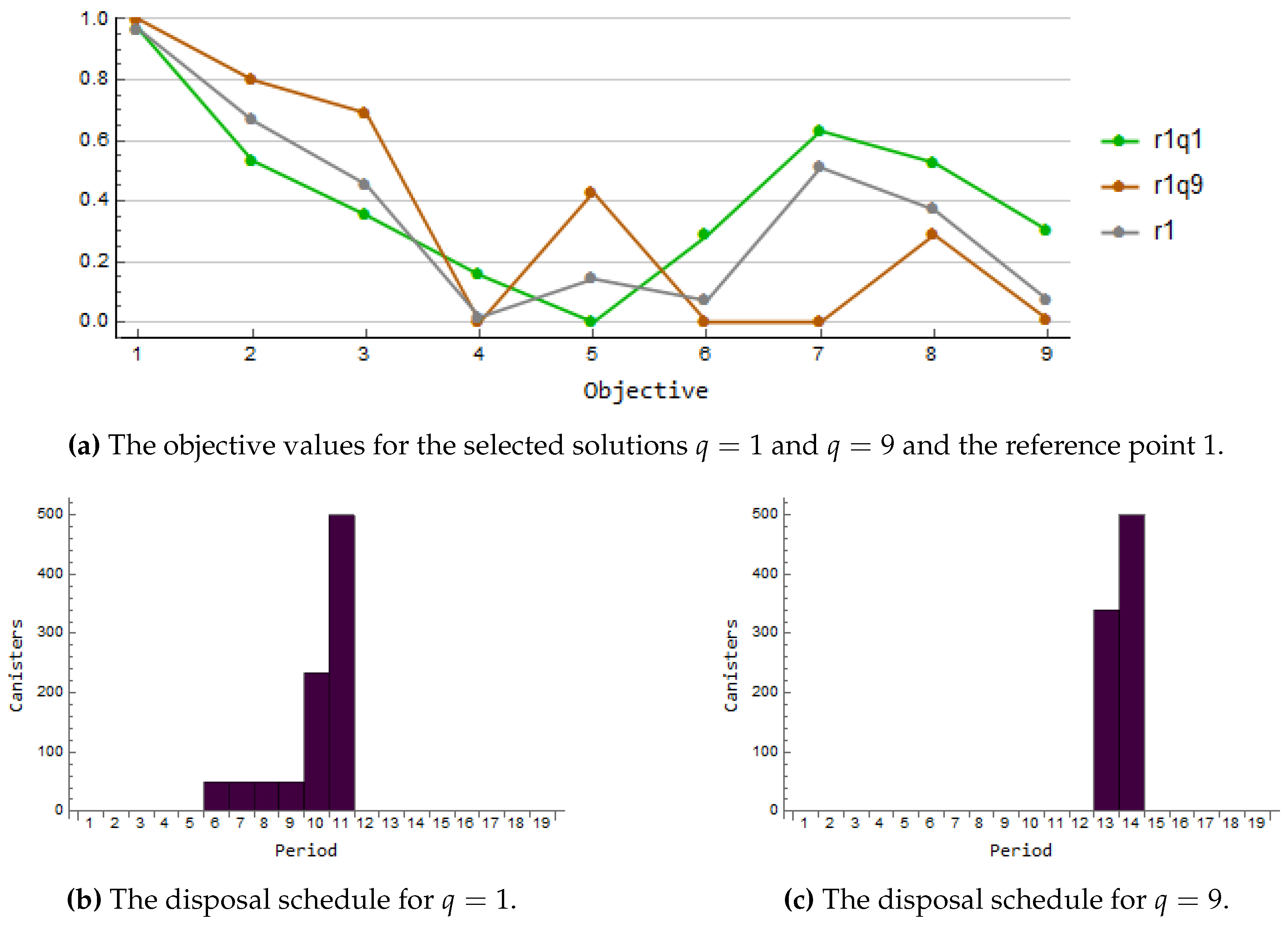
Figure 3.
Results for the iteration 2.

Figure 4.
Results for the iteration 3.

Figure 5.
The objective values corresponding the selected solutions and for the modified reference point 3 with objectives (1)–(8).
Figure 5.
The objective values corresponding the selected solutions and for the modified reference point 3 with objectives (1)–(8).

Figure 6.
Results for the iteration 4.
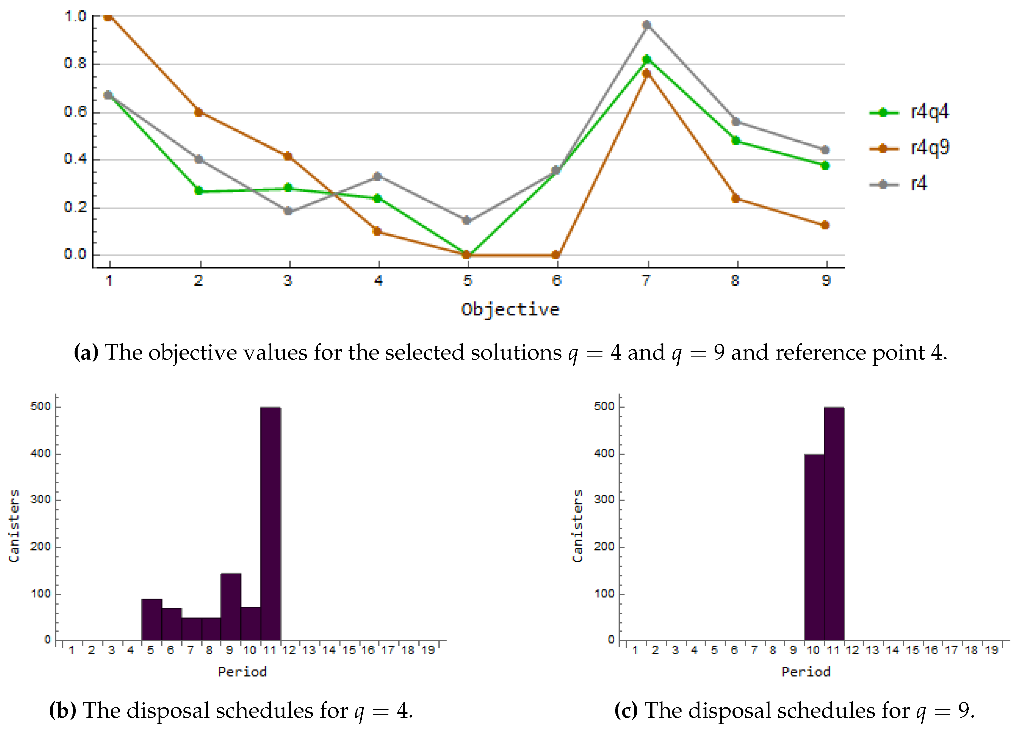
Figure 7.
The four solutions where disposal starts early.

Figure 8.
The four solutions where disposal starts late.

© 2019 by the authors. Licensee MDPI, Basel, Switzerland. This article is an open access article distributed under the terms and conditions of the Creative Commons Attribution (CC BY) license (http://creativecommons.org/licenses/by/4.0/).
Share and Cite
MDPI and ACS Style
Montonen, O.; Ranta, T.; Mäkelä, M.M. Planning the Schedule for the Disposal of the Spent Nuclear Fuel with Interactive Multiobjective Optimization. Algorithms 2019, 12, 252. https://doi.org/10.3390/a12120252
AMA Style
Montonen O, Ranta T, Mäkelä MM. Planning the Schedule for the Disposal of the Spent Nuclear Fuel with Interactive Multiobjective Optimization. Algorithms. 2019; 12(12):252. https://doi.org/10.3390/a12120252
Chicago/Turabian StyleMontonen, Outi, Timo Ranta, and Marko M. Mäkelä. 2019. "Planning the Schedule for the Disposal of the Spent Nuclear Fuel with Interactive Multiobjective Optimization" Algorithms 12, no. 12: 252. https://doi.org/10.3390/a12120252
Note that from the first issue of 2016, this journal uses article numbers instead of page numbers. See further details here.