Decision Tree Methods for Predicting Surface Roughness in Fused Deposition Modeling Parts


Department of Mechanical Engineering, University of Cordoba, Medina Azahara Avenue, 5–14071 Cordoba, Spain
*
Author to whom correspondence should be addressed.
Materials 2019, 12(16), 2574; https://doi.org/10.3390/ma12162574
Submission received: 20 July 2019
/
Revised: 8 August 2019
/
Accepted: 12 August 2019
/
Published: 12 August 2019
(This article belongs to the Special Issue Industrial Additive Manufacturing Process Planning: Process Evaluation, Metrology, and Post-Processing Techniques)
Abstract
:3D printing using fused deposition modeling (FDM) includes a multitude of control parameters. It is difficult to predict a priori what surface finish will be achieved when certain values are set for these parameters. The objective of this work is to compare the models generated by decision tree algorithms (C4.5, random forest, and random tree) and to analyze which makes the best prediction of the surface roughness in polyethylene terephthalate glycol (PETG) parts printed in 3D using the FDM technique. The models have been created using a dataset of 27 instances with the following attributes: layer height, extrusion temperature, print speed, print acceleration, and flow rate. In addition, a dataset has been created to evaluate the models, consisting of 15 additional instances. The models generated by the random tree algorithm achieve the best results for predicting the surface roughness in FDM parts.
1. Introduction
Additive manufacturing or 3D printing techniques allow small batches of parts to be produced directly, economically, and flexibly [1]. There are different additive manufacturing techniques; however, fused deposition modeling (FDM) printers are the most extended due to their low cost and the wide variety of materials that can be used [2,3,4].
FDM printers offer a large number of print parameters: print temperature, layer height, print speed, print acceleration, and flow rate, among others. When a part is printed, it is difficult to predict a priori if it will receive an adequate surface finish [5,6].
Data mining techniques are used to improve the quality of processes and products based on data gathered from previous experiences [7,8,9]: they are used to find out which parameters are most influential in surface finishing in electrical discharge machining (EDM) processes [10]. They are also used to predict the wear of a tool in milling processes [11] or to increase the accuracy of high-speed machining of titanium alloys [12].
Data mining techniques can be classified into supervised (classification, regression) and unsupervised (clustering, association rules, correlations). Classification techniques are widely utilized [9]. To use these techniques, different classes must be established in which each instance in the database must belong to a class; the rest of the attributes of the instance are used to predict that class. The objective of these algorithms is to maximize the accuracy ratio of the classification of new instances [13].
Decision trees are one of the most widely used classification techniques in data mining [13]. Tree nodes represent a condition relative to a given attribute. The leaves indicate the number of instances that belong to a class and that satisfy the conditions imposed in the previous nodes. By means of this type of algorithms, it is possible to create models that allow for predictions such as whether a register with certain attributes will belong to one class or another. There are several classification algorithms: C4.5 [14], random forest [15], random tree [16].
Previous work has focused on the use of classification techniques in additive manufacturing processes. Wu et al. [17,18] applied random forest, k-nearest neighbor, and anomaly detection techniques to detect defects caused by a cyberattack on an FDM printer during part fabrication. Amini and Chang [19] used classification techniques to reduce defects in metal parts manufacturing processes using selective laser melting (SLM) printers. Recently, Li et al. [20] have generated and checked models using different machine learning algorithms to predict the surface roughness of 3D printed parts using FDM; in this case, the authors used a design of experiments with three variables (layer height, print temperature, and print speed/flow rate) and measured the roughness in a unique direction.
The objective of this work is to analyze which decision tree algorithm (C4.5, random forest, or random tree) is the best to predict the surface finish (Ra,0 and Ra,90) of a FDM printed part. Data mining models have been developed from a training dataset consisting of 27 instances with attributes of layer height, print temperature, flow rate, print speed, print acceleration, Ra,0 class, and Ra,90 class. These models have been tested using a dataset with 15 additional instances.
2. Materials and Methods
Figure 1 shows the different stages that constitute the methodology followed in this work: 3D printing, surface roughness measurements, data mining, models generation, models testing, and comparison between algorithms.
2.1. 3D Printing and Surface Roughness Measurements
To carry out the present study, 27 specimens of dimensions 25.0 mm × 25.0 mm × 2.4 mm were printed, following a design of fractionated orthogonal experiments, with five factors and three levels. The parameters used and the values assigned to each level are shown in Table 1.
The specimens were designed using SolidWorks software. The selection of values for print parameters and numerical code (NC) generation was done using CURA software. The specimens were manufactured using an Ender 3 printer, with a diameter nozzle equal to 0.4 mm.
The polyethylene terephthalate glycol (PETG) filament was supplied by Smart Materials 3D (Smart Materials 3D, Alcalá la Real, Spain). Although there are not many published works on PETG, it is a filament increasingly used in the industry, having mechanical characteristics similar to ABS but printed with the ease of a PLA [21].
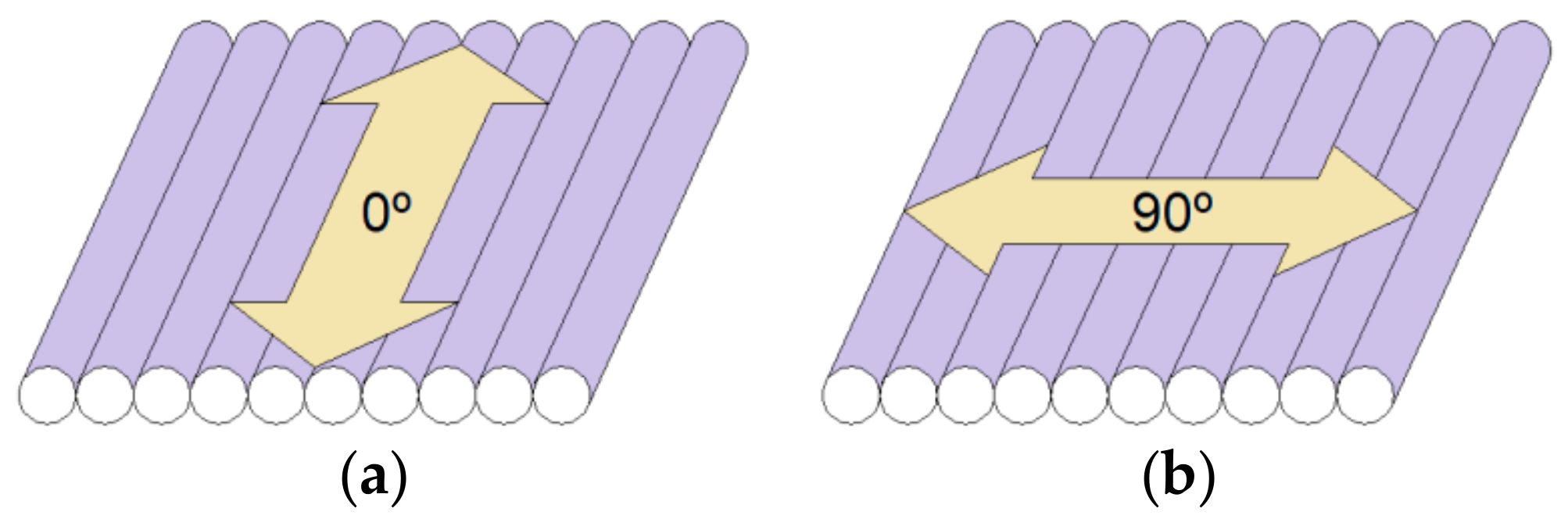
Once printed, the roughness of the specimens was measured using a Mitutoyo perthometer model SJ-201 (Mitutoyo, Kawasaki, Japan). Five measurements were made in each specimen and direction, 0° and 90°, as seen in Figure 2. The representative value was calculated as the arithmetic mean of the five measurements. The resulting values are shown in Table 2.
The models were generated using the free software WEKA (Waikato Environment for Knowledge Analysis). The roughness values were divided into two classes (class 1 and class 2) from the mean of the values of Ra,0 and Ra,90. For Ra,0, class 1 includes 0–4.43 μm and class 2 is from 4.43 to 10.64 μm. For Ra,90, class 1 includes 0–11.63 μm and class 2 includes 11.63–32.99 μm. To validate the model obtained, 15 additional specimens were printed using random values for the parameters under study, as seen in Table 3. Likewise, five roughness measurements were performed on each specimen and direction, obtaining the representative values by means of the arithmetic mean.
2.2. Data Mining and Decision Trees
The data mining process consists of several steps: (1) integration and data collection, which coincides with the previous paragraph; (2) selection, cleaning and transformation, in which the data were prepared in .arff format, which are files used by WEKA; (3) data mining, consisting of applying the algorithms to the data and generating patterns and models; (4) evaluation and interpretation of the information generated; (5) generation of knowledge and decision making.
In this work, three algorithms based on decision trees are compared: J48 (a variation of WEKA for C4.5), random forest, and random tree. The algorithms are briefly presented below.
2.2.1. J48 (C4.5)
The J48 is WEKA’s version of the C4.5 algorithm. Algorithm C4.5, created by Quinlan [14], allows the generation of decision trees. It is an iterative algorithm that consists of dividing the data in each stage into two groups using the concept of information entropy. This partitioning process is recursive and stops when all records of a sheet belong to the same class or category.
2.2.2. Random Forest
The random forest method was developed by Breiman [15]. It consists of constructing multiple decision trees using random combinations and orders of variables before constructing a random tree using bootstrap aggregating (also known as bagging). This highly accurate algorithm is capable of handling hundreds of variables without excluding any [16].
2.2.3. Random Tree
The random tree is an algorithm halfway between a simple decision tree and a random forest. Random trees are a set of predictor trees called forest. The classification mechanisms are as follows: the random tree classifier obtains the input characteristic vector, classifies it with each tree in the forest, and produces the class label that received the most “votes” [13].
3. Results
This work proposes the use of decision trees and data mining techniques to predict which values should be selected for the print parameters of PETG flat specimens, manufactured by FDM. The dataset used as a training dataset to develop the models is shown in Table 4.
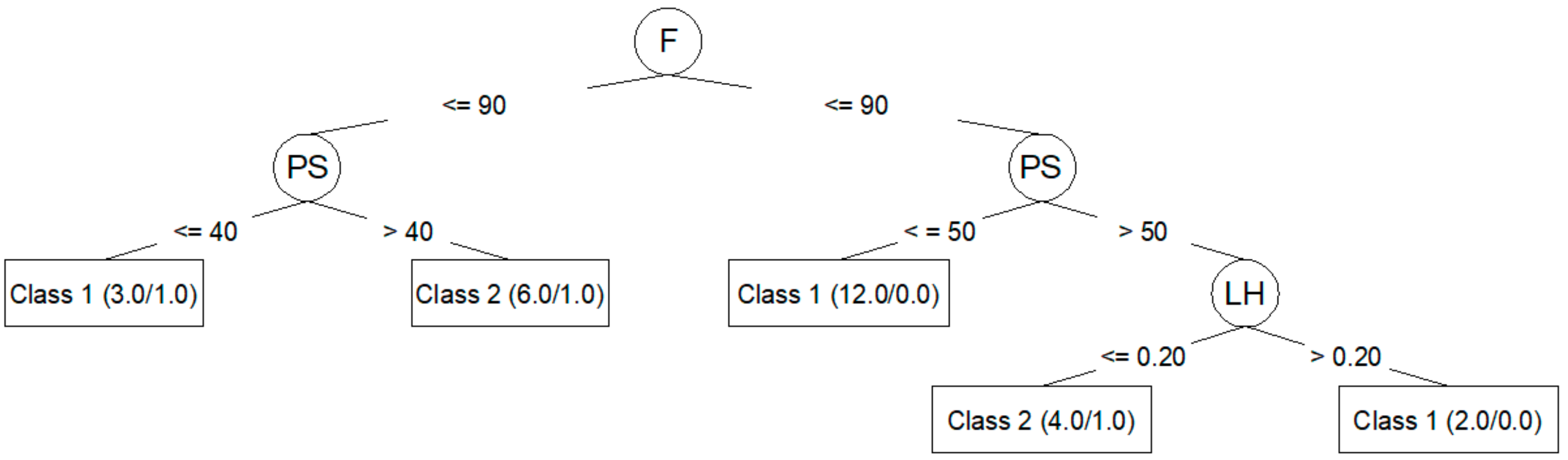
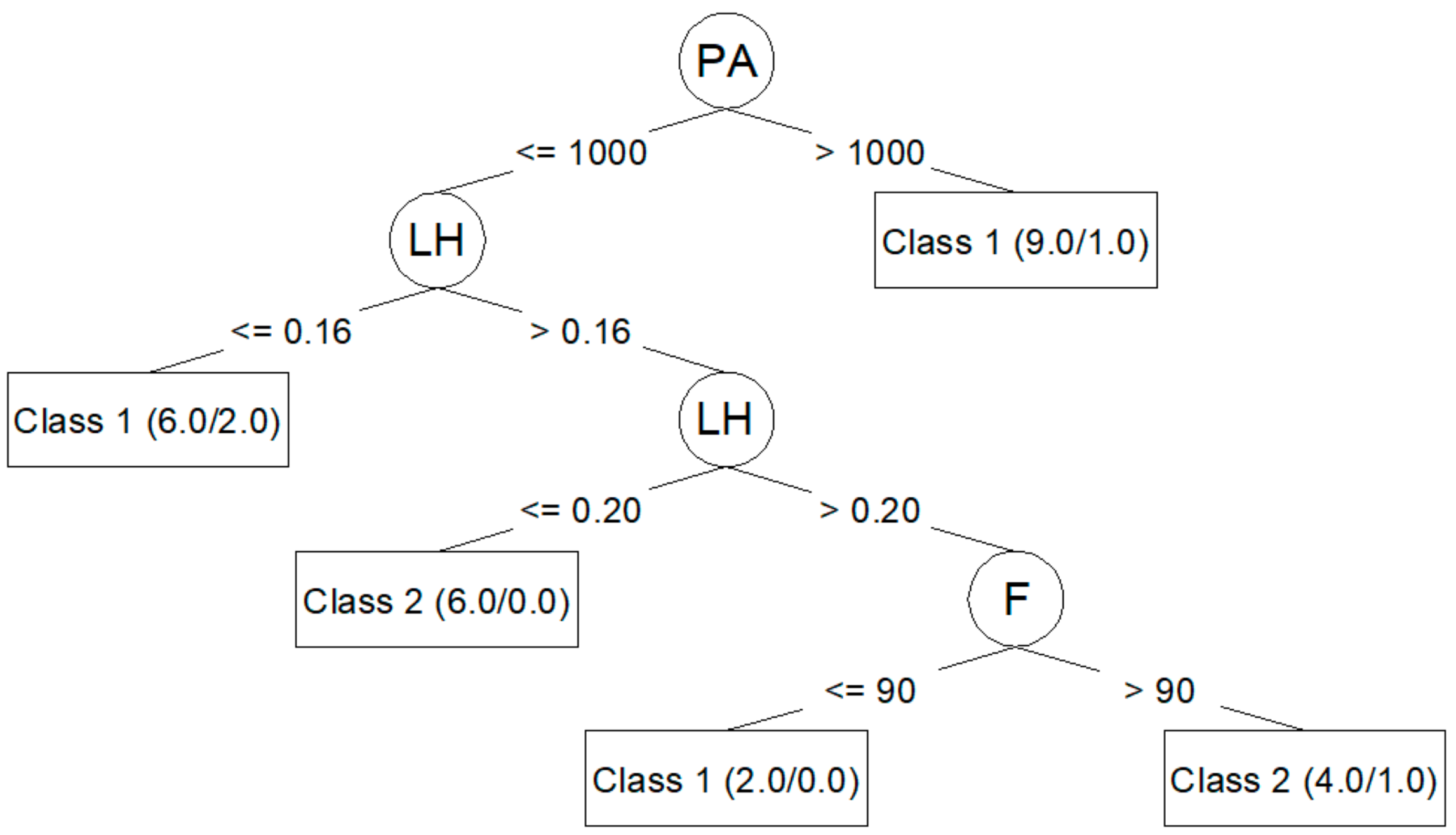
Algorithm J48 (C4.5) generates decision trees that can be represented graphically. Figure 3 shows the decision tree generated for Ra,0 from the corresponding training dataset. Figure 4 shows the decision tree generated for Ra,90.
Once the models have been generated using the algorithms studied, they have been checked using the dataset shown in Table 5. The results of each algorithm for the prediction of Ra,0 are shown in Table 6 and Table 7. Likewise, the results for the prediction of Ra,90 are presented in Table 8 and Table 9. Table 10 shows the time used by each algorithm to construct and validate the models.
The J48 algorithm allows for the generation of simple trees that can be easily understood and interpreted, as seen in Figure 3 and Figure 4. In these trees, it is clear which parameters are most important to reduce Ra,0 (PA, LH, F) and Ra,90 (F, PS, LH). However, the models created by means of the J48 algorithm are those that adjust the worst to the test data, as seen in Table 6 and Table 8: a 60.00% success rate for Ra,0; a 73.33% success rate for Ra,90; and a negative kappa statistic in both cases. Table 7 and Table 9 show that the precision for the models created using the J48 algorithm is lower than that achieved by the rest of the models, and that the value of the area under the ROC is very low.
The random forest algorithm slightly improves the results of J48, as seen in Table 6 and Table 8; the model created using this algorithm provides 66.67% success for Ra,0 and 80.00% success for Ra,90. In this case, the kappa statistic is close to zero for Ra,0 and negative for Ra,90. Table 7 and Table 9 show that the precision of both models increases, as does the area under ROC. This algorithm does not generate trees that can be plotted.
The models generated by the random tree algorithm are the ones that obtain the best results in this case, as seen in Table 6 and Table 8, with an 80% success rate for Ra,0 and 86.67% success rate for Ra,90. It obtains a positive kappa statistic in both cases: 0.2857 for Ra,0 and 0.5946 for Ra,90. These values can be classified as fair and moderate according to Table 11. Table 7 and Table 9 show that the precision of both models is higher than in the cases analyzed above; the area under ROC is 0.673 for the Ra,0 model and 0.923 for the Ra,90 model. In addition, as can be seen in Table 10, this algorithm took the least time to build the models.
4. Discussion
In the present work, three classification tree algorithms were used to predict the surface finish of FDM-printed PETG flat specimens. The algorithms used were J48, random forest, and random tree. The software used to generate the models was WEKA [13].
The J48 algorithm has been widely used to study problems in the manufacturing area related to quality improvement in production processes [10,22]. In this work, the J48 generated models that classified training dataset data very well. Additionally, this algorithm made it possible to create trees that can be plotted and that are easily understood [10,16,23,24]. This algorithm also allowed for the identification of the most influential parameters in roughness: PA, LH, and F for Ra,0; F, PS, and LH for Ra,90. These results coincide with those obtained by the authors in previous works [25]: PA is the parameter with the greatest influence on Ra,0; F, PS, and LH are the parameters with the greatest influence on Ra,90. However, in this case, the models created with J48 algorithm were not able to predict the data used in the test. This may be related to overfitting problems [13,26].
5. Conclusions
In the present work, three models were created and compared to predict the surface roughness of flat pieces printed on PETG by FDM. For this purpose, data mining classification were used, such as J48 (C4.5), random forest, and random tree. The software used to generate the models was the open source software WEKA.
The model generated by random tree obtains better results. It correctly classifies a priori 80% of the instances in the case of Ra,0 and 86.67% of the instances in the case of Ra,90. It is the only algorithm of the three evaluated that achieves a positive kappa statistic, qualified as fair for Ra,0 and moderate for Ra,90. It obtains the highest accuracy and area under ROC and is also the fastest algorithm of the three analyzed.
In future works, we intend to study whether the decision trees can be used to generate models that allow for the prediction of a better dimensional accuracy of the parts manufactured by FDM. The impact of other print factors on the surface properties of printed parts, such as nozzle diameter, will also be studied.
Author Contributions
Conceptualization, P.E.R.; methodology, P.E.R.; software, P.E.R.; validation, J.M.B. and P.E.R.; formal analysis, P.E.R.; investigation, J.M.B.; resources, P.E.R.; data curation, J.M.B.; writing—original draft preparation, J.M.B.; writing—review and editing, P.E.R.; visualization, J.M.B.; supervision, P.E.R.; project administration, P.E.R.; funding acquisition, P.E.R.
Funding
This research was funded by University of Cordoba, via “Plan Propio de Investigacion”.
Acknowledgments
The authors would like to thank Smart Materials 3D (www.smartmaterials3d.com) for the material supplied. We must also thank the laboratory technician Ana Martin Bernal for her help during the work.
Conflicts of Interest
The authors declare no conflict of interest.
References
- Lipson, H.; Kurman, M. Fabricated: The New World of 3D Printing; John Wiley & Sons Inc.: Indianapolis, IN, USA, 2013. [Google Scholar]
- Carneiro, O.S.; Silva, A.F.; Gomes, R. Fused deposition modeling with polypropylene. Mater. Des. 2015, 83, 768–776. [Google Scholar] [CrossRef]
- Ahn, S.; Montero, M.; Odel, D.; Roundy, S.; Wright, P.K. Anisotropic material properties of fused deposition modeling ABS. Rapid Prototyp. J. 2002, 8, 248–257. [Google Scholar] [CrossRef] [Green Version]
- Messimer, S.L.; Pereira, T.R.; Patterson, A.E.; Lubna, M.; Drozda, F.O. Full-density fused deposition modeling dimensional error as a function of raster angle and build orientation: Large dataset for eleven materials. J. Manuf. Mater. Process. 2019, 3, 6. [Google Scholar] [CrossRef]
- Nancharaiah, T.; Raju, D.R.; Raju, V.R. An experimental investigation on surface quality and dimensional accuracy of FDM components. Int. J. Emerg. Technol. 2010, 1, 106–111. [Google Scholar]
- Gordon, E.R.; Shokrani, A.; Flynn, J.M.; Goguelin, S.; Barclay, J.; Dhokia, V. A Surface Modification Decision Tree to Influence Design in Additive Manufacturing. In Sustainable Design and Manufacturing 2016. SDM2016. Smart Innovation, Systems and Technologies; Setchi, R., Howlett, R., Liu, Y., Theobald, P., Eds.; Springer: Cham, Switzerland, 2016; Volume 52, ISBN 9783319320984. [Google Scholar]
- Harding, J.A.; Shahbaz, M.; Srinivas, S.; Kusiak, A. Data Mining in Manufacturing: A review. J. Manuf. Sci. Eng. 2006, 128, 969–976. [Google Scholar] [CrossRef]
- Choudhary, A.K.; Harding, J.A.; Tiwari, M.K. Data mining in manufacturing: A review based on the kind of knowledge. J. Intell. Manuf. 2009, 20, 501–521. [Google Scholar] [CrossRef]
- Köksal, G.; Batmaz, I.; Testik, M.C. A review of data mining applications for quality improvement in manufacturing industry. Expert Syst. Appl. 2011, 38, 13448–13467. [Google Scholar] [CrossRef]
- Kuriakose, S.; Mohan, K.; Shunmugam, M.S. Data mining applied to wire-EDM process. J. Mater. Process. Technol. 2003, 142, 182–189. [Google Scholar] [CrossRef]
- Wu, D.; Jennings, C.; Terpenny, J.; Gao, R.X.; Kumara, S. A comparative study on machine learning algorithms for smart manufacturing: Tool wear prediction using random forests. J. Manuf. Sci. Eng. 2017, 139, 071018. [Google Scholar] [CrossRef]
- Krishnakumar, P.; Rameshkumar, K.; Ramachandran, K.I. Acoustic Emission-Based Tool Condition Classification in a Precision High-Speed Machining of Titanium Alloy: A machine learning approach. Int. J. Comput. Intell. Appl. 2018, 17, 1850017. [Google Scholar] [CrossRef]
- Witten, I.H.; Frank, E.; Hall, M.A. Data Mining: Practical Machine Learning Tools and Techniques, 3rd ed.; Morgan Kaufmann: Burlington, MA, USA, 2011. [Google Scholar]
- Quinlan, J.R. C4.5: Programs for Machine Learning; Morgan Kaufmann Publishers, Inc.: San Mateo, CA, USA, 2014. [Google Scholar]
- Breiman, L. Random forest. Mach. Learn. 2001, 45, 5–32. [Google Scholar] [CrossRef]
- Zhao, Y.; Zhang, Y. Comparison of decision tree methods for finding active objects. Adv. Space Res. 2008, 41, 1955–1959. [Google Scholar] [CrossRef]
- Wu, M.; Song, Z.; Moon, Y.B. Detecting cyber-physical attacks in CyberManufacturing systems with machine learning methods. J. Intell. Manuf. 2019, 30, 1111–1123. [Google Scholar] [CrossRef]
- Wu, M.; Zhou, H.; Lin, L.L.; Silva, B.; Song, Z.; Cheung, J.; Moon, Y. Detecting attacks in cybermanufacturing systems: Additive manufacturing example. MATEC Web Confer. 2017, 108, 06005. [Google Scholar] [CrossRef]
- Amini, M.; Chang, S.I. MLCPM: A process monitoring framework for 3D metal printing in industrial scale. Comput. Ind. Eng. 2018, 124, 322–330. [Google Scholar] [CrossRef]
- Li, Z.; Zhang, Z.; Shi, J.; Wu, D. Prediction of surface roughness in extrusion-based additive manufacturing with machine learning. Robot. Comput. Integr. Manuf. 2019, 57, 488–495. [Google Scholar] [CrossRef]
- Smart Materials 3D. Available online: https://www.smartmaterials3d.com/en/ (accessed on 17 January 2019).
- Kim, A.; Oh, K.; Jung, J.; Kim, B. Imbalanced classification of manufacturing quality conditions using cost-sensitive decision tree ensembles. Int. J. Comput. Integr. Manuf. 2017, 31, 701–717. [Google Scholar] [CrossRef]
- Ronowicz, J.; Thommes, M.; Kleinebudde, P.; Krysiński, J. A data mining approach to optimize pellets manufacturing process based on a decision tree algorithm. Eur. J. Pharm. Sci. 2015, 73, 44–48. [Google Scholar] [CrossRef]
- Rodríguez, J.; Quintana, G.; Bustillo, A.; Ciurana, J. A decision-making tool based on decision trees for roughness prediction in face milling. Int. J. Comput. Integr. Manuf. 2017, 30, 943–957. [Google Scholar] [CrossRef]
- Barrios, J.M.; Romero, P.E. Improvement of surface roughness and hydrophobicity in PETG parts manufactured via fused deposition modeling (FDM): An application in 3D printed self—Cleaning parts. Materials (Basel) 2019, 12, 2499. [Google Scholar] [CrossRef]
- Rokach, L. Decision forest: Twenty years of research. Inf. Fusion 2016, 27, 111–125. [Google Scholar] [CrossRef]
- Sathyadevan, S.; Nair, R.R. Comparative Analysis of Decision Tree Algorithms: ID3, C4.5 and Random Forest. In Computational Intelligence in Data Mining—Volume 1. Smart Innovation, Systems and Technologies; Jain, L., Behera, H., Mandal, J., Mohapatra, D., Eds.; Springer: New Delhi, India, 2015; Volume 31, pp. 549–562. ISBN 9788132222057. [Google Scholar]
- Kwon, B.; Won, J.; Kang, D. Fast Defect Detection for Various Types of Surfaces using Random Forest with VOV Features. Int. J. Precis. Eng. Manuf. 2015, 16, 965–970. [Google Scholar] [CrossRef]
- Ali, J.; Khan, R.; Ahmad, N.; Maqsood, I. Random Forests and Decision Trees. Int. J. Comput. Sci. Issues 2012, 9, 272–278. [Google Scholar]
- Amand, B.; Cordy, M.; Heymans, P.; Acher, M.; Temple, P.; Jézéquel, J. Towards learning-aided configuration in 3D printing: Feasibility study and application to defect prediction. In Proceedings of the 13th International Workshop on Variability Modelling of Software Intensive Systems (VaMoS’19), Leuven, Belgium, 6–8 February 2019; Perrouin, G., Weyns, D., Eds.; ACM: New York, NY, USA, 2019; p. 9. [Google Scholar]
- Kevric, J.; Jukic, S.; Subasi, A. An effective combining classifier approach using tree algorithms for network intrusion detection. Neural Comput. Appl. 2017, 28, 1051–1058. [Google Scholar] [CrossRef]
- Ravichandran, S.; Srinivasan, V.B.; Ramasamy, C. Comparative study on decision tree techniques for mobile call detail record. J. Commun. Comput. 2012, 9, 1331–1335. [Google Scholar]
Figure 1.
Different stages that compose the methodology followed in the present work: 3D printing, surface roughness measurements, data mining, models generation, models testing, and comparison between algorithms.
Figure 1.
Different stages that compose the methodology followed in the present work: 3D printing, surface roughness measurements, data mining, models generation, models testing, and comparison between algorithms.
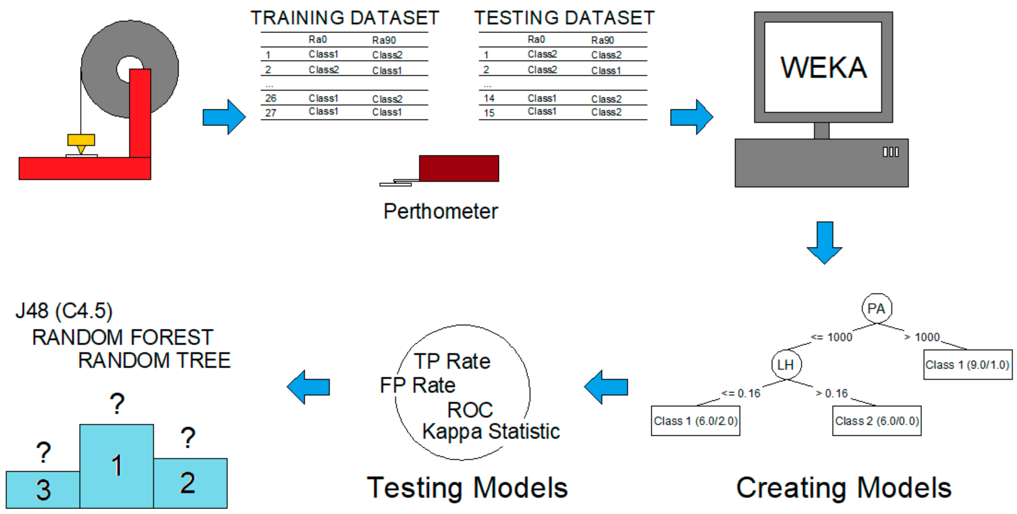
Figure 2.
Measurement of surface roughness in the direction parallel to the direction of extrusion (a) and in the direction perpendicular to the direction of extrusion (b).
Figure 2.
Measurement of surface roughness in the direction parallel to the direction of extrusion (a) and in the direction perpendicular to the direction of extrusion (b).

Figure 3.
J48 (C4.5) decision tree for Ra,0.

Figure 4.
J48 (C4.5) decision tree for Ra,90.

Table 1.
Factors and levels used in design of the experiments (DOE).
| Print Parameter | Level 1 | Level 2 | Level 3 |
|---|---|---|---|
| Layer height (LH), mm | 0.16 | 0.20 | 0.24 |
| Temperature (T), °C | 240 | 245 | 250 |
| Print speed (PS), mm/s | 40 | 50 | 60 |
| Print acceleration (PA), mm/s2 | 500 | 1000 | 1500 |
| Flow rate (F), % | 90 | 100 | 110 |
Table 2.
Training dataset: design of experiment (L27), according to Taguchi method: layer height (LH), print temperature (T), print speed (PS), print acceleration (PA), and flow rate (F).
Table 2.
Training dataset: design of experiment (L27), according to Taguchi method: layer height (LH), print temperature (T), print speed (PS), print acceleration (PA), and flow rate (F).
| No. | LH (mm) | T (°C) | PS (mm/s) | PA (mm/s2) | F (%) |
|---|---|---|---|---|---|
| 1 | 0.16 | 240 | 40 | 500 | 90 |
| 2 | 0.16 | 240 | 40 | 500 | 100 |
| 3 | 0.16 | 240 | 40 | 500 | 110 |
| 4 | 0.16 | 245 | 50 | 1000 | 110 |
| 5 | 0.16 | 245 | 50 | 1000 | 90 |
| 6 | 0.16 | 245 | 50 | 1000 | 100 |
| 7 | 0.16 | 250 | 60 | 1500 | 100 |
| 8 | 0.16 | 250 | 60 | 1500 | 110 |
| 9 | 0.16 | 250 | 60 | 1500 | 90 |
| 10 | 0.20 | 240 | 50 | 1500 | 100 |
| 11 | 0.20 | 240 | 50 | 1500 | 110 |
| 12 | 0.20 | 240 | 50 | 1500 | 90 |
| 13 | 0.20 | 245 | 60 | 500 | 90 |
| 14 | 0.20 | 245 | 60 | 500 | 100 |
| 15 | 0.20 | 245 | 60 | 500 | 110 |
| 16 | 0.20 | 250 | 40 | 1000 | 110 |
| 17 | 0.20 | 250 | 40 | 1000 | 90 |
| 18 | 0.20 | 250 | 40 | 1000 | 100 |
| 19 | 0.24 | 240 | 60 | 1000 | 110 |
| 20 | 0.24 | 240 | 60 | 1000 | 90 |
| 21 | 0.24 | 240 | 60 | 1000 | 100 |
| 22 | 0.24 | 245 | 40 | 1500 | 100 |
| 23 | 0.24 | 245 | 40 | 1500 | 110 |
| 24 | 0.24 | 245 | 40 | 1500 | 90 |
| 25 | 0.24 | 250 | 50 | 500 | 90 |
| 26 | 0.24 | 250 | 50 | 500 | 100 |
| 27 | 0.24 | 250 | 50 | 500 | 110 |
Table 3.
Test dataset: design of experiment (L27), according to Taguchi method: layer height (LH), print temperature (T), print speed (PS), print acceleration (PA), and flow rate (F).
Table 3.
Test dataset: design of experiment (L27), according to Taguchi method: layer height (LH), print temperature (T), print speed (PS), print acceleration (PA), and flow rate (F).
| No. | LH (mm) | T (°C) | PS (mm/s) | PA (mm/s2) | F (%) |
|---|---|---|---|---|---|
| 1 | 0.14 | 240 | 15 | 200 | 95 |
| 2 | 0.14 | 236 | 18 | 300 | 105 |
| 3 | 0.18 | 238 | 15 | 300 | 115 |
| 4 | 0.18 | 243 | 20 | 200 | 95 |
| 5 | 0.14 | 246 | 35 | 400 | 105 |
| 6 | 0.23 | 248 | 46 | 400 | 95 |
| 7 | 0.24 | 243 | 45 | 600 | 103 |
| 8 | 0.30 | 230 | 56 | 2000 | 100 |
| 9 | 0.30 | 250 | 60 | 1600 | 110 |
| 10 | 0.20 | 251 | 70 | 1500 | 102 |
| 11 | 0.20 | 249 | 85 | 1200 | 100 |
| 12 | 0.28 | 249 | 100 | 1200 | 98 |
| 13 | 0.28 | 237 | 25 | 1100 | 90 |
| 14 | 0.14 | 238 | 21 | 800 | 100 |
| 15 | 0.10 | 239 | 50 | 600 | 110 |
Table 4.
Training dataset: results for surface roughness (Ra,0, Ra,90).
| Test | Ra,0 (µm) | Ra,0 Class | Ra,90 (µm) | Ra,90 Class |
|---|---|---|---|---|
| 1 | 10.648 | Class2 | 12.240 | Class2 |
| 2 | 0.916 | Class1 | 6.464 | Class1 |
| 3 | 1.126 | Class1 | 9.160 | Class1 |
| 4 | 2.428 | Class1 | 32.994 | Class2 |
| 5 | 1.800 | Class1 | 5.504 | Class1 |
| 6 | 8.814 | Class2 | 10.922 | Class1 |
| 7 | 4.552 | Class2 | 23.650 | Class2 |
| 8 | 1.370 | Class1 | 14.458 | Class2 |
| 9 | 0.954 | Class1 | 5.414 | Class1 |
| 10 | 1.462 | Class1 | 23.470 | Class2 |
| 11 | 1.666 | Class1 | 9.050 | Class1 |
| 12 | 1.554 | Class1 | 10.074 | Class1 |
| 13 | 6.258 | Class2 | 20.088 | Class2 |
| 14 | 7.788 | Class2 | 15.368 | Class2 |
| 15 | 10.172 | Class2 | 12.560 | Class2 |
| 16 | 9.744 | Class2 | 10.186 | Class2 |
| 17 | 4.696 | Class2 | 5.462 | Class1 |
| 18 | 5.112 | Class2 | 5.330 | Class1 |
| 19 | 4.274 | Class2 | 10.668 | Class1 |
| 20 | 6.994 | Class1 | 8.214 | Class1 |
| 21 | 5.868 | Class2 | 6.056 | Class1 |
| 22 | 3.796 | Class2 | 8.680 | Class1 |
| 23 | 3.054 | Class1 | 5.720 | Class1 |
| 24 | 3.702 | Class1 | 6.804 | Class1 |
| 25 | 4.124 | Class1 | 19.654 | Class1 |
| 26 | 4.682 | Class1 | 8.964 | Class2 |
| 27 | 2.256 | Class2 | 7.122 | Class1 |
Table 5.
Testing dataset: results for surface roughness (Ra,0, Ra,90).
| Test | Ra,0 (µm) | Ra,0 Class | Ra,90 (µm) | Ra,90 Class |
|---|---|---|---|---|
| 1 | 1.026 | Class1 | 4.462 | Class1 |
| 2 | 1.178 | Class1 | 2.656 | Class1 |
| 3 | 2.064 | Class1 | 3.97 | Class1 |
| 4 | 1.126 | Class1 | 7.192 | Class1 |
| 5 | 1.984 | Class1 | 9.24 | Class1 |
| 6 | 1.252 | Class1 | 8.276 | Class1 |
| 7 | 1.026 | Class1 | 4.462 | Class1 |
| 8 | 1.744 | Class1 | 7.732 | Class1 |
| 9 | 5.906 | Class2 | 11.408 | Class1 |
| 10 | 3.99 | Class1 | 12.082 | Class2 |
| 11 | 1.182 | Class1 | 6.392 | Class1 |
| 12 | 1.008 | Class1 | 6.622 | Class1 |
| 13 | 6.466 | Class2 | 14.002 | Class2 |
| 14 | 0.606 | Class1 | 6.828 | Class1 |
| 15 | 1.846 | Class1 | 4.758 | Class1 |
Table 6.
Indicators to compare the models generated by the studied algorithms to predict Ra,0.
| Indicator | J48 | Random Forest | Random Tree |
|---|---|---|---|
| Correctly Classified Instances | 60.00% | 66.67% | 80.00% |
| Incorrectly Classified Instances | 40.00% | 33.33% | 20.00% |
| Kappa statistic | −0.2162 | 0.1176 | 0.2857 |
| Mean absolute error | 0.4926 | 0.429 | 0.2 |
| Root mean squared error | 0.595 | 0.474 | 0.4472 |
| Relative absolute error | 106.60% | 92.84% | 43.28% |
| Root relative squared error | 128.39% | 102.29% | 96.50% |
Table 7.
Detailed precision parameters achieved by each algorithm for the Ra,0 prediction model.
| Detailed Accuracy (weighted av.) | J48 | Random Forest | Random Tree |
|---|---|---|---|
| True Positive (TP) Rate | 0.600 | 0.667 | 0.800 |
| False Positive (FP) Rate | 0.908 | 0.474 | 0.454 |
| Precision | 0.709 | 0.807 | 0.839 |
| Recall | 0.600 | 0.667 | 0.800 |
| F-measure | 0.650 | 0.716 | 0.816 |
| MCC | −0.237 | 0.139 | 0.294 |
| ROC Area | 0.154 | 0.692 | 0.673 |
| PRC Area | 0.697 | 0.868 | 0.819 |
Table 8.
Indicators to compare the models generated by the studied algorithms to predict Ra,90.
| Indicator | J48 | Random Forest | Random Tree |
|---|---|---|---|
| Correctly Classified Instances | 73.33% | 80.00% | 86.67% |
| Incorrectly Classified Instances | 26.67% | 20.00% | 13.33% |
| Kappa statistic | −0.1538 | −0.0976 | 0.5946 |
| Mean absolute error | 0.2556 | 0.2888 | 0.1333 |
| Root mean squared error | 0.4645 | 0.3854 | 0.3651 |
| Relative absolute error | 66.17% | 74.57% | 34.52% |
| Root relative squared error | 116.01% | 96.26% | 91.20% |
Table 9.
Detailed precision parameters achieved by each algorithm for the Ra,90 prediction model.
| Detailed Accuracy (weighted av.) | J48 | Random Forest | Random Tree |
|---|---|---|---|
| True Positive (TP) Rate | 0.733 | 0.800 | 0.867 |
| False Positive (FP) Rate | 0.887 | 0.877 | 0.021 |
| Precision | 0.733 | 0.743 | 0.933 |
| Recall | 0.733 | 0.800 | 0.867 |
| F-measure | 0.733 | 0.770 | 0.883 |
| MCC | −0.154 | −0.105 | 0.650 |
| ROC Area | 0.385 | 0.481 | 0.923 |
| PRC Area | 0.745 | 0.797 | 0.916 |
Table 10.
Time used by each algorithm to build and validate the model.
| Algorithm | Computing Time for Ra,0 Model (s) | Computing Time for Ra,90 Model (s) |
|---|---|---|
| J48 | 0.11 | 0.19 |
| Random Forest | 0.05 | 0.34 |
| Random Tree | 0.01 | 0.01 |
Table 11.
Strength of concordance for kappa statistic.
| Kappa Statistic | Strength of Concordance |
|---|---|
| 0.00 | Poor |
| 0.01–0.20 | Slight |
| 0.21–0.40 | Fair |
| 0.41–0.60 | Moderate |
| 0.61–0.80 | Substancial |
| 0.81–1.00 | Almost perfect |
© 2019 by the authors. Licensee MDPI, Basel, Switzerland. This article is an open access article distributed under the terms and conditions of the Creative Commons Attribution (CC BY) license (http://creativecommons.org/licenses/by/4.0/).
Share and Cite
MDPI and ACS Style
Barrios, J.M.; Romero, P.E. Decision Tree Methods for Predicting Surface Roughness in Fused Deposition Modeling Parts. Materials 2019, 12, 2574. https://doi.org/10.3390/ma12162574
AMA Style
Barrios JM, Romero PE. Decision Tree Methods for Predicting Surface Roughness in Fused Deposition Modeling Parts. Materials. 2019; 12(16):2574. https://doi.org/10.3390/ma12162574
Chicago/Turabian StyleBarrios, Juan M., and Pablo E. Romero. 2019. "Decision Tree Methods for Predicting Surface Roughness in Fused Deposition Modeling Parts" Materials 12, no. 16: 2574. https://doi.org/10.3390/ma12162574
Note that from the first issue of 2016, this journal uses article numbers instead of page numbers. See further details here.