Drivability-Related Discrete-Time Model Predictive Control of Mode Transition in Pre-Transmission Parallel Hybrid Powertrains

Abstract

During the mode transition from the pure electric propulsion mode to the hybrid propulsion mode, clutch-based pre-transmission parallel hybrid electric vehicles are subject to drivability issues. These issues originate from the fact that in the clutch-based pre-transmission parallel hybrid powertrain (CPPHP) configuration, the clutch connects the engine and the motor. Without a carefully designed mode transition control that coordinates the engine torque, clutch torque and motor torque, torque sluggishness and surges occur during the mode transition, and residual torque oscillation occurs after the mode transition. In this paper, a discrete-time model predictive control (DMPC)-based controller is proposed to address these drivability-related issues. Modeling improvements and novel drivability-related indices and constraints are all taken into consideration in the design of the discrete-time model predictive controller. Furthermore, by using discrete-time Laguerre functions and introducing the equilibrium state and the ranking of constraints, an explicit solution of the discrete-time model predictive controller is obtained. The calculation results demonstrate that the proposed controller can ensure a smooth and rapidly decaying torque difference during the mode transition, alleviating the residual torque oscillation after the mode transition and guaranteeing that the mode transition is completed within an acceptable duration.

1. Introduction

In comparison with conventional powertrains driven only by internal combustion engines, hybrid powertrains augment fuel efficiency and significantly reduce emissions [1]. Three typical hybrid powertrain architectures are widely used in hybrid electric vehicles (HEVs) on the market: planetary gear set based series-parallel hybrids [2], clutch-based series-parallel hybrids [3] and clutch-based parallel hybrids [4]. These configurations are schematically depicted in Figure 1.

The clutch-based pre-transmission parallel hybrid is the most cost-effective type of hybrid powertrain configuration among the aforementioned three [5]. Numerous studies on clutch-based pre-transmission parallel hybrid powertrains (CPPHPs) have focused on energy management [6] and emissions control [7]. Nevertheless, during the mode transition from the pure electric propulsion mode to the hybrid propulsion mode, drivability-related issues emerge in CPPHPs due to the clutch engagement. Within the finite duration of this process, multiple objectives need to be accomplished simultaneously: adjusting the engine and motor torques to their respective target values determined by the energy management system, sustaining a low level of torque difference between the supplied by the hybrid power source and the demanded by the driver during the mode transition, achieving a smooth clutch engagement at the ending of the mode transition and ensuring a low level of residual torque oscillation after the mode transition. These are the most significant challenges when designing a mode transition controller.

Conventionally, vehicle manufacturers define drivability as the driver’s subjective perception of the vehicle’s powertrain operation. Hence, studies have been devoted to identifying the correlation between measurable vehicle powertrain response indices and the quantification of the driver’s subjective perception [8]. Furthermore, commercial test tools such as AVL Drive (AVL LIST GmbH, Hans-List-Platz 1, Graz, Austria) can automatically measure a vehicle’s powertrain response indices and then infer the overall drivability rating [9]. In this paper, we primarily discuss the design of the mode transition controller, and therefore the term ‘drivability’ directly denotes a vehicle’s powertrain response indices. These indices reflect a vehicle’s powertrain response characteristics to the driver’s maneuvers: sluggishness, surge and oscillation [10]. The most commonly used vehicle powertrain response indices are the duration and the responsiveness and smoothness of the vehicle’s longitudinal acceleration [11,12]. Given that the external resistance can be considered to be constant during the mode transition, the responsiveness and smoothness of the vehicle’s longitudinal acceleration are equivalent to those of the propulsion torque exerted on the drivetrain by the hybrid power source. Hence, in this paper, we choose the responsiveness and smoothness of the propulsion torque output by the hybrid power source in combination with the duration of the mode transition as the vehicle’s powertrain response indices instead of those of the vehicle’s longitudinal acceleration. The process of clutch engagement is composed of the preparation phase, the inertia phase and the post phase, as illustrated in Figure 2.

In a CPPHP, the inertia phase is the mode transition from the pure electric propulsion mode to the hybrid propulsion mode. Hence, the key to excellent mode transition control is coordinating the engine torque, clutch torque and motor torque to accomplish the aforementioned multiple objectives simultaneously during the inertia phase. Various approaches based on classical and modern control theories have been used to solve the torque coordination control problem. Koprubasi et al. proposed an output feedback control based asymptotic stable controller to smooth the clutch engagement in the CPPHP [13]. Kim et al. presented a disturbance compensation based torque coordination control strategy to alleviate the torque oscillation during the inertia phase in a CPPHP [14]. Chen et al. introduced an output feedback control based torque coordination controller to achieve a smooth clutch engagement at the ending of the inertia phase in the clutch-based pre-transmission series-parallel hybrid powertrain [15]. Kum et al. designed a dynamic programming based engine-start controller to quickly start the engine during the inertia phase in the CPPHP [16].

Torque coordination during the mode transition involves clutch control issues, and the partial objectives are identical to those of clutch control in automated manual transmissions and dual clutch transmissions. Many studies have proposed different solutions for clutch control issues. Dolcini et al. implemented a quadratic programming based lurch avoidance clutch control strategy in an automated manual transmission prototype [17]. Walker and Zhang designed a proportional-integral-derivative controller using the speed difference between the differential and the wheel as the input to suppress the residual torque oscillation after the inertia phase of an up shift [18]. Lu et al. proposed a data-driven predictive control based gearshift control strategy to track the clutch speed difference reference trajectory by manipulating the oncoming clutch torque and engine output torque during the inertia phase of a clutch-to-clutch shift [19].

Model predictive control is adept at managing multiple objective optimization problems with constraints. Some studies have presented model predictive controllers to solve the torque coordination control problem during the mode transition in CPPHPs. Beck et al. designed a model predictive control based triple controller to coordinate the engine and motor torques during the clutch engagement [20]. Pisaturo et al. utilized a composite model predictive controller to track the predefined trajectories of the engine speed and clutch speed during the inertia phase in an automated manual transmission. Numerical results validated this controller in critical operating conditions with constraints [21].

The aforementioned studies give valuable insights into the torque coordination control problem during the mode transition in CPPHPs. However, the following details can be improved: the stiffness and damping of the elastic components included in the hybrid powertrain should be modeled; the response characteristics of the engine, clutch and motor should be modeled; in the clutch inertia phase control, the responsiveness of the propulsion torque output by the hybrid power source should be regarded as one drivability-related index; and before the instant of the clutch engagement, the clutch sliding speed and speed difference between the differential and the wheel should be minimized simultaneously because the speed difference between the differential and the wheel results in residual torque oscillation.

These modeling improvements and novel drivability-related indices and constraints are all taken into consideration in the design of the discrete-time model predictive controller in this paper. These elements haven’t been comprehensively and systematically taken into account in other relevant studies before, whereas these details indeed influence drivability.

Modeling the stiffness and damping of the elastic components included in the hybrid powertrain is the key to capturing the residual torque oscillation during the post phase; modeling the response characteristics of the engine, clutch and motor is the key to describing the change of the propulsion torque output by the hybrid power source during the inertia phase; the responsiveness of the propulsion torque output by the hybrid power source is the key index to evaluate drivability during the inertia phase; the clutch sliding speed influences the torque step at the instant of the clutch engagement; and the speed difference between the differential and the wheel influences the residual torque oscillation during the post phase. These are important and necessary for drivability during the whole process of the clutch engagement, so should be contemplated comprehensively.

Furthermore, by using discrete-time Laguerre functions and introducing the equilibrium state and the ranking of constraints, an explicit solution of the discrete-time model predictive controller is obtained in this paper. The explicit solution can simplify the programming and guarantee the existence of the solution of the optimization problem. Consequently, the explicit solution benefits the attempt to implement the designed discrete-time model predictive controller on an embedded micro control unit in future studies. The key parameters of the discrete-time model predictive controller are determined by comparison with a discrete-time linear quadratic regulator (DLQR) minimizing the almost identical cost function but without constraints.

The outline of this paper is as follows: Section 2 describes the configuration of the CPPHP discussed in this paper; Section 3 describes the simulation-oriented and control-oriented models of the CPPHP; Section 4 details the design of the discrete-time model predictive controller; the parameters and performance of the designed controller are discussed in Section 5 and conclusions are drawn in Section 6.

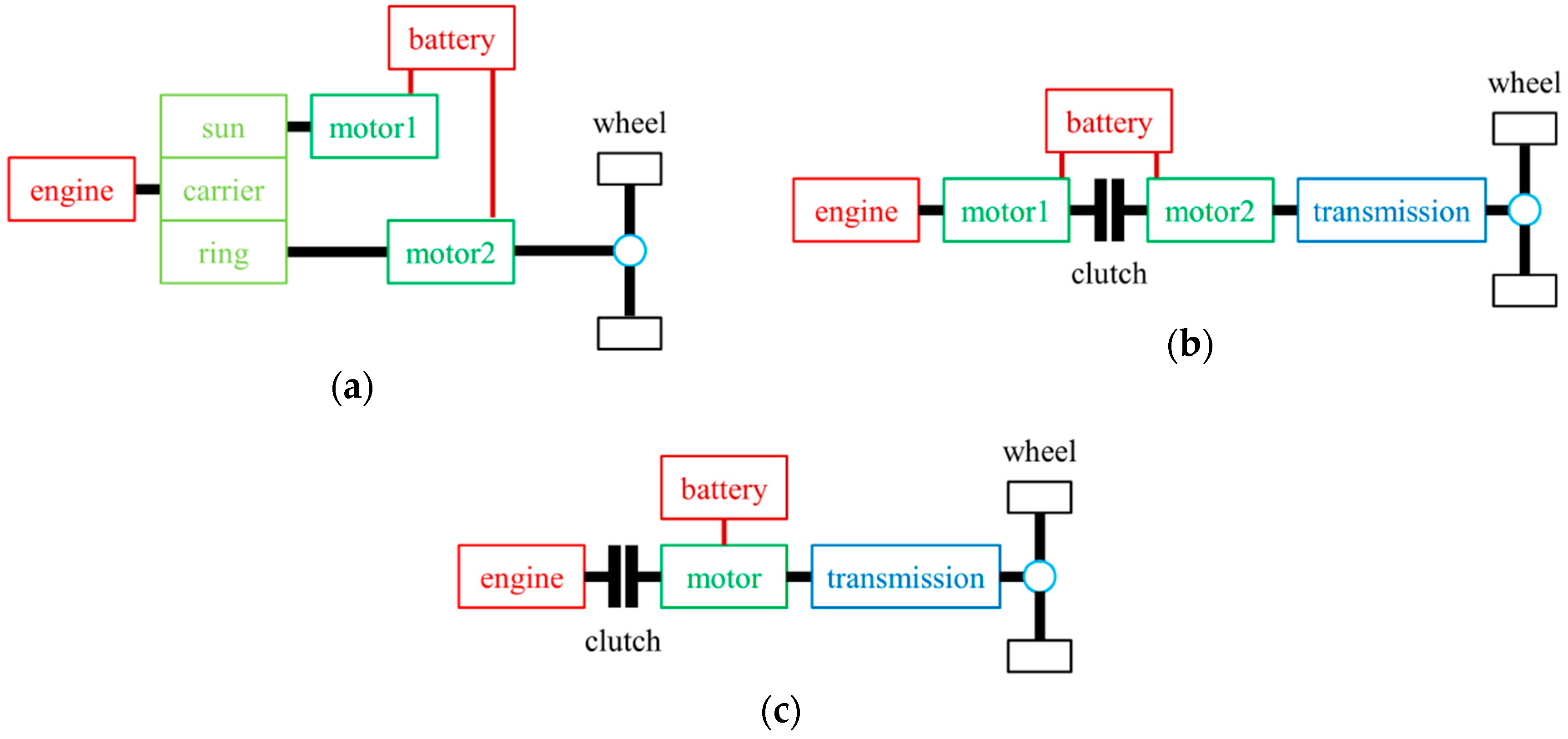
2. Powertrain Configuration

The CPPHP schematically depicted in Figure 1c is primarily composed of the engine, clutch, motor, transmission, final drive, differential, axle shafts, tires and related accessories. In comparison with the conventional powertrain configuration with an automatic transmission, the CPPHP configuration substitutes a clutch for the torque converter and incorporates a motor into the primary shaft of the transmission. Other necessary components that must be added to the powertrain include the battery, motor drive and corresponding controllers. Obviously, most components and technologies of the conventional powertrain apply to the CPPHP, and structure-related issues include how to arrange the clutch and the motor in the compact space. Bosch and FEV have completely addressed this issue and produced respective transmission integration solutions.

3. Powertrain Modeling

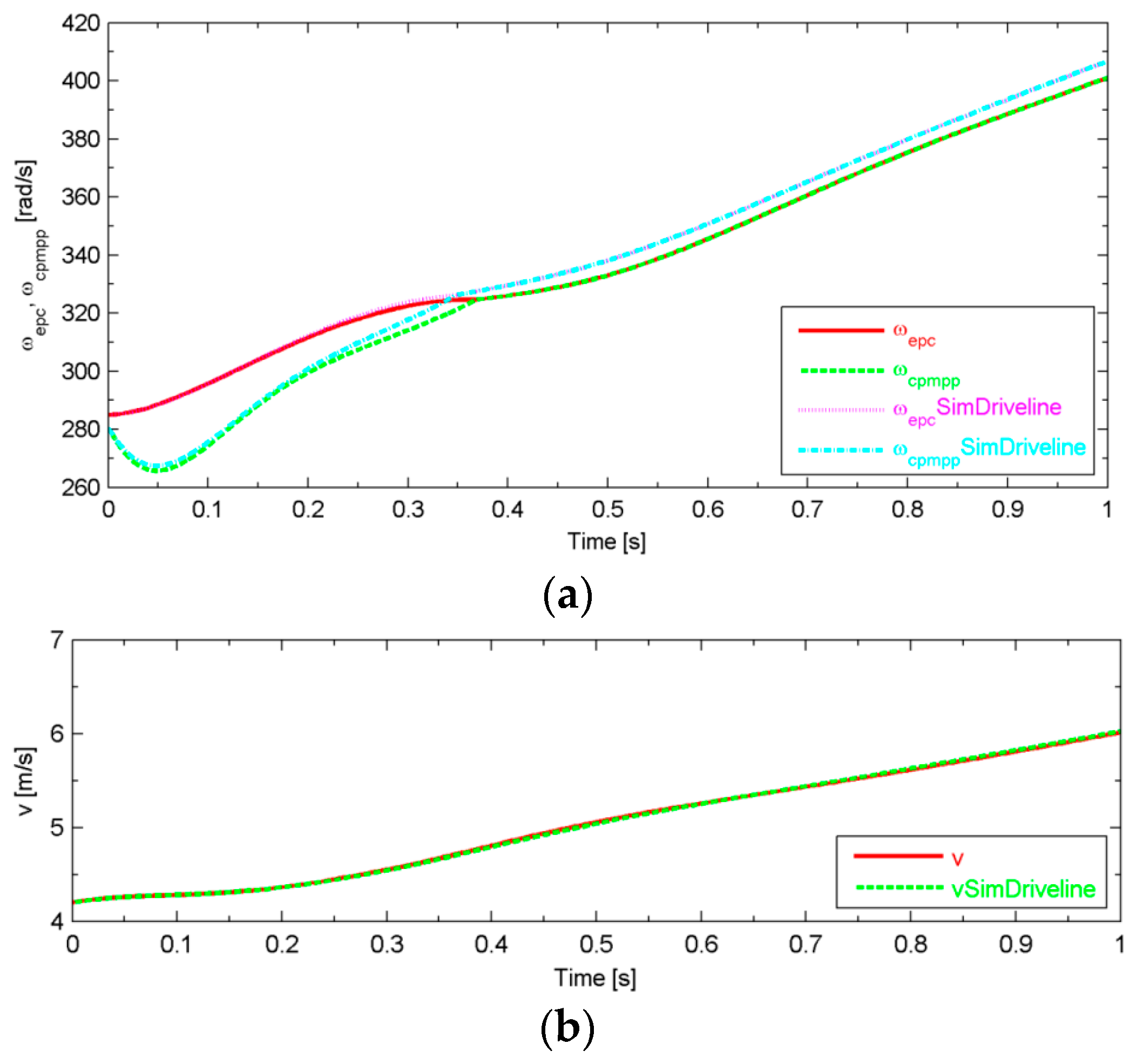
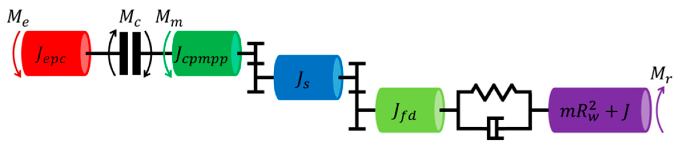
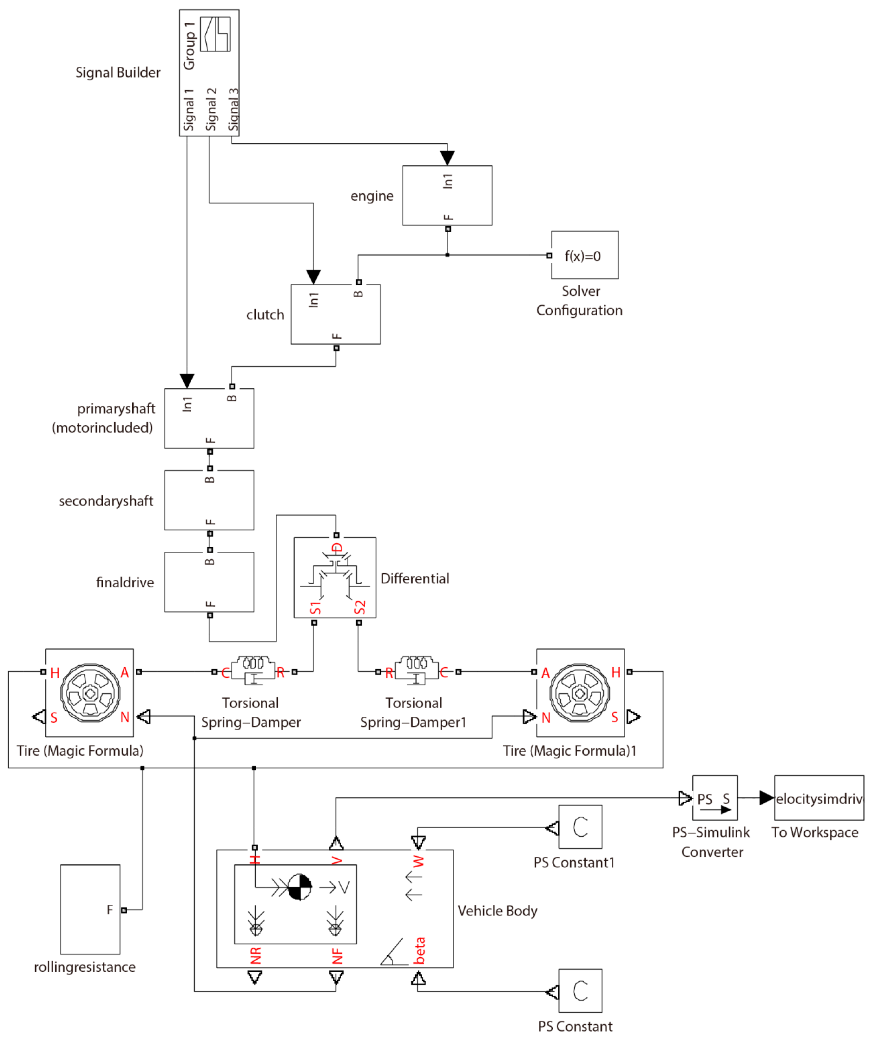
3.1. Simulation-Oriented Model

The simulation-oriented model describes the dynamics of the main components of the CPPHP as comprehensively as possible and functions as the plant in the simulation. The simulation-oriented model will be simplified later to derive the control-oriented model. The dynamics model of the CPPHP is illustrated in Figure 3.

3.1.1. Engine

The response characteristics of the internal combustion engine can be modeled by a first order system with a time constant ${\tau }_e$. Thus, the engine output torque $M_e$ is calculated by:

$${\dot{M}}_e=-\frac{1}{{\tau }_e}{M}_e+\frac{1}{{\tau }_e}{M}_{ec}$$

(1)

with the engine time constant ${\tau }_e$ and the engine output torque command $M_{ec}$. The rotational components of the engine and the associated driving parts of the clutch can be modeled as a lumped moment of inertia $J_{epc}$. The rotational speed of this lumped moment of inertia ${\omega }_{epc}$ is computed by:

$${\dot{\omega }}_{epc}=\frac{1}{J_{epc}}{M}_e-\frac{1}{J_{epc}}{M}_c$$

(2)

with the lumped moment of inertia $J_{epc}$, the engine output torque $M_e$ and the torque transmitted by the clutch $M_c$.

3.1.2. Clutch

The clutch functions as a torque coupler in the CPPHP. The clutch actuator can be modeled by a first order system with a time constant ${\tau }_c$. Then, the normalized normal force $r_c$ is calculated by:

$${\dot{r}}_c=-\frac{1}{{\tau }_c}{r}_c+\frac{1}{{\tau }_c}{r}_{cc}$$

(3)

with the clutch actuator time constant ${\tau }_c$ and the normalized normal force command $r_{cc}$. Here $r_c\in \left[0,1\right]$ and $r_{cc}\in \left[0,1\right]$. The clutch can be modeled by a LuGre friction model. Different from the hybrid models usually adopted in the literature, the LuGre friction model is a continuous non-linear model [22]. Thus, the clutch is modeled as:

$${\dot{z}}_c=-\frac{\left|R_c\left({\omega }_{epc}-{\omega }_{cpmpp}\right)\right|}{g_c\left({\omega }_{epc},{\omega }_{cpmpp}\right)}{z}_c+R_c\left({\omega }_{epc}-{\omega }_{cpmpp}\right)$$

(4)

$$g_c\left({\omega }_{epc},{\omega }_{cpmpp}\right)=\frac{1}{{\sigma }_0}\left[F_{Coulomb}+\left(F_{stiction}-F_{Coulomb}\right)e^{-{\left(\frac{\left|R_c\left({\omega }_{epc}-{\omega }_{cpmpp}\right)\right|}{v_{Stribeck}}\right)}^{0.9}}\right]$$

(5)

$$M_c={\sigma }_0{r}_c{z}_c{R}_c+{\sigma }_1{r}_c{\dot{z}}_c{R}_c+{\sigma }_2{r}_c{R}_c\left({\omega }_{epc}-{\omega }_{cpmpp}\right)R_c$$

(6)

where $z_c$ denominates the average deflection of the bristles, $R_c$ the equivalent radius of the clutch, ${\omega }_{epc}$ the rotational speed of the lumped moment of inertia $J_{epc}$, ${\omega }_{cpmpp}$ the rotational speed of $J_{cpmpp}$, $J_{cpmpp}$ the lumped moment of inertia of the driven parts of the clutch, the rotor of the motor and the primary shaft of the transmission, ${\mathsf{\sigma }}_0$ the stiffness coefficient, $F_{Coulomb}$ the Coulomb force, $F_{stiction}$ the stiction force, $v_{Stribeck}$ the Stribeck velocity, $M_c$ the torque transmitted by the clutch, $r_c$ the normalized normal force, ${\mathsf{\sigma }}_1$ the microscopic damping coefficient and ${\mathsf{\sigma }}_2$ the macroscopic damping coefficient. By using the Matlab functions ‘max’ and ‘min’, the normalized normal force command $r_{cc}$ is computed by:

$$r_{cc}=\{\begin{array}{c}\text{max}\left(0,\min \left(1,\frac{M_{cc}}{{\sigma }_0{g}_c\left({\omega }_{epc},{\omega }_{cpmpp}\right)R_c+{\sigma }_2{R}_c\left({\omega }_{epc}-{\omega }_{cpmpp}\right)R_c}\right)\right), {\omega }_{epc}>{\omega }_{cpmpp}\\ \text{max}\left(0,\min \left(1,\frac{M_{cc}}{F_{stiction}{R}_c}\right)\right), {\omega }_{epc}={\omega }_{cpmpp}\\ \text{max}\left(0,\min \left(1,\frac{-M_{cc}}{{\sigma }_0{g}_c\left({\omega }_{epc},{\omega }_{cpmpp}\right)R_c+{\sigma }_2{R}_c\left({\omega }_{cpmpp}-{\omega }_{epc}\right)R_c}\right)\right), {\omega }_{epc}<{\omega }_{cpmpp}\end{array}$$

(7)

with the clutch torque command $M_{cc}$.

3.1.3. Motor

The motor between the clutch and the transmission in the pre-transmission parallel hybrid powertrain architecture is the other power source of the hybrid powertrain. The response characteristics of the motor can be modeled by a first order system with a time constant ${\tau }_m$. Then, the motor output torque $M_m$ is calculated by:

$${\dot{M}}_m=-\frac{1}{{\tau }_m}{M}_m+\frac{1}{{\tau }_m}{M}_{mc}$$

(8)

with the motor time constant ${\tau }_m$ and the motor output torque command $M_{mc}$.

3.1.4. Transmission

The transmission used in the CPPHP can be modeled as rigid gear pairs. The driven parts of the clutch, the rotor of the motor and the primary shaft of the transmission can be modeled as a lumped moment of inertia $J_{cpmpp}$. The rotational speed of this lumped moment of inertia ${\omega }_{cpmpp}$ is computed by:

$${\dot{\omega }}_{cpmpp}=\frac{1}{J_{cpmpp}}\left(M_c+M_m-M_s\right)$$

(9)

with the lumped moment of inertia $J_{cpmpp}$, the torque transmitted by the clutch $M_c$, the motor output torque $M_m$ and the torque exported from the primary shaft $M_s$. The secondary shaft of the transmission can be modeled as a lumped moment of inertia $J_s$. Generally, in terms of the state of the clutch, the primary modes of the CPPHP consist of the pure electric propulsion mode, the hybrid propulsion mode and the regenerative braking mode. When torque demanded by the driver is positive, the CPPHP is switched to the pure electric propulsion mode or the hybrid propulsion mode; and when torque demanded by the driver is negative, the CPPHP is switched to the regenerative braking mode. In the pure electric propulsion mode and the hybrid propulsion mode, the torque exported from the primary shaft $M_s$ is positive and for a given $M_s$, the external resistance torque $M_r$ results in acceleration or deceleration. In the regenerative braking mode, the clutch is open and the torque exported from the primary shaft $M_s$ is negative.

In this paper, we primarily discuss the mode transition from the pure electric propulsion mode to the hybrid propulsion mode and this is the key mode transition of the clutch-based pre-transmission parallel hybrid electric vehicles. During this mode transition, ideally, the propulsion torque exported from the primary shaft $M_s$ by the hybrid power source (the engine and the motor) should sustain unchanged by applying a well-designed controller. Hence, although the motor output torque may be negative, the total propulsion torque exported from the primary shaft $M_s$ by the hybrid power source (the engine and the motor) will sustain positive and the direction of the power flow is from the hybrid power source to the drivetrain. Therefore, the rotational speed of this lumped moment of inertia ${\omega }_s$ is calculated by:

$${\dot{\omega }}_s=\frac{1}{J_s}\left(i_g{\eta }_g{M}_s-M_{fd}\right)$$

(10)

with the lumped moment of inertia $J_s$, the gear ratio $i_g$, the transmission efficiency ${\mathsf{\eta }}_g$, the torque exported from the primary shaft $M_s$, and the torque exported from the secondary shaft $M_{fd}$. ${\omega }_{cpmpp}$ and ${\omega }_s$ are linked by:

$${\omega }_s=\frac{{\omega }_{cpmpp}}{i_g}$$

(11)

3.1.5. Final Drive

Assuming that driving axle shafts rotate at identical speeds, the final drive and the differential can be modeled as a pair of gears. They can be modeled as a lumped moment of inertia $J_{fd}$, and given that the direction of the power flow is from the hybrid power source to the drivetrain during the mode transition, the rotational speed of this lumped moment of inertia ${\omega }_{fd}$ is computed by:

$${\dot{\omega }}_{fd}=\frac{1}{J_{fd}}\left(i_{fd}{\eta }_{fd}{M}_{fd}-M_{as}\right)$$

(12)

with the lumped moment of inertia $J_{fd}$, the final drive ratio $i_{fd}$, the final drive efficiency ${\mathsf{\eta }}_{fd}$, the torque exported from the secondary shaft $M_{fd}$ and the torque transmitted by the axle shafts $M_{as}$. ${\omega }_s$ and ${\omega }_{fd}$ are linked by:

$${\omega }_{fd}=\frac{{\omega }_s}{i_{fd}}$$

(13)

3.1.6. Driving Axle Shaft

Driving axle shafts can be modeled by an equivalent elastic shaft as:

$$\dot{\theta }={\omega }_{fd}-{\omega }_w$$

(14)

$$M_{as}=k\theta +b\left({\omega }_{fd}-{\omega }_w\right)$$

(15)

where $\theta$ denotes the torsion of the axle shaft, ${\omega }_{fd}$ the rotational speed of the lumped moment of inertia $J_{fd}$, ${\omega }_w$ the wheel rotational speed, $M_{as}$ the torque transmitted by the axle shafts, $k$ the equivalent stiffness coefficient and $b$ the equivalent damping coefficient.

3.1.7. Longitudinal Vehicle Dynamics

Assuming that there is no slip between the tires and the road, in accordance with the power equation, the dynamics of the vehicle is modeled as [23]:

$${\dot{\omega }}_w=\frac{1}{m{R}_w^2+J}\left(M_{as}-M_r\right)$$

(16)

$$M_r=\left(mg \text{cos} \alpha C_{rr}+\frac{1}{2}{C}_{D}A\rho v^2+mg \text{sin} \alpha \right)R_w$$

(17)

$$v=R_w{\omega }_w$$

(18)

where ${\omega }_w$ denominates the wheel rotational speed, $m$ the vehicle mass, $R_w$ the wheel radius, $J$ the entire moment of inertia of the vehicle body and the tires, $M_{as}$ the torque transmitted by the axle shafts, $M_r$ the external resistance torque, $g$ the gravitational acceleration, $\alpha$ the road slope, $C_{rr}$ the rolling resistance coefficient, $C_D$ the drag coefficient, $A$ the frontal area, $\mathsf{\rho }$ the air density and $v$ the vehicle longitudinal velocity.

The engine, clutch actuator and motor time constants are set to be reasonable values of the correct order of magnitude by analyzing the mean value model of the engine, by referencing data provided by the manufacturer, and based on a preliminary test of a permanent magnet synchronous motor respectively. The equivalent radius of the clutch is calculated based on the specifications provided by the manufacturer. The Coulomb force, Stiction force, Stribeck velocity and macroscopic damping coefficient are determined by fitting the LuGre friction model to the characteristic curves provided by the manufacturer. The stiffness coefficient and microscopic damping coefficient are determined by analyzing the characteristics of the LuGre friction model in the literature [22]. The moment of inertia of the rotational components of the engine and the parameters of the transmission, final drive, driving axle shafts and longitudinal vehicle dynamics models are determined by referencing the values of that in the literature [24,25] and by collecting the available specifications of the vehicle. The parameters of the simulation-oriented model are shown in

Table 1. Parameters of the simulation-oriented model.

Description	Symbol	Value
Engine time constant	${\tau }_e$	0.1 s
Lumped moment of inertia of the engine and the driving parts of the clutch	$J_{epc}$	0.15 kg·m2
Equivalent radius of the clutch	$R_c$	0.1 m
Coulomb force	$F_{Coulomb}$	348.4 N
Stiction force	$F_{stiction}$	1636.1 N
Stribeck velocity	$v_{Stribeck}$	22 m/s
Macroscopic damping coefficient	${\mathsf{\sigma }}_2$	0.001 Ns/m
Clutch actuator time constant	${\mathsf{\tau }}_c$	0.01 s
Stiffness coefficient	${\mathsf{\sigma }}_0$	108 N/m
Microscopic damping coefficient	${\mathsf{\sigma }}_1$	106 Ns/m
Motor time constant	${\mathsf{\tau }}_m$	0.001 s
Lumped moment of inertia of the driven parts of the clutch, the rotor of the motor and the primary shaft of the transmission	$J_{cpmpp}$	0.05 kg·m2
Gear ratio	$i_g$	4
Transmission efficiency	${\mathsf{\eta }}_g$	0.98
Lumped moment of inertia of the secondary shaft of the transmission	$J_s$	0.01 kg·m2
Final drive ratio	$i_{fd}$	5
Final drive efficiency	${\mathsf{\eta }}_{fd}$	0.98
Lumped moment of inertia of the final drive and the differential	$J_{fd}$	0.01 kg·m2
Equivalent stiffness coefficient of the axle shafts	$k$	6000 Nm/rad
Equivalent damping coefficient of the axle shafts	$b$	400 Nms/rad
Vehicle mass	$m$	1250 kg
Entire moment of inertia of the vehicle body and the tires	$J$	10 kg·m2
Wheel radius	$R_w$	0.3 m
Rolling resistance coefficient	$C_{rr}$	0.01
Gravitational acceleration	$g$	9.8 m/s2
Road slope	$\alpha$	0
Drag coefficient	$C_D$	0.3
Frontal area	$A$	2 m2
Air density	$\mathsf{\rho }$	1.25 kg/m3

.

The simulation result of a Matlab SimDriveline (The MathWorks, Inc., Natick, MA, USA) model is used to validate the proposed model. The model depicted in Figure 4 is based on the standard component models provided by the Matlab SimDriveline.

The scenario to be simulated is: the engine output torque command $M_{ec}$ steps from 0 Nm to 60 Nm at the beginning of the simulation; the initial engine output torque $M_{e0}$ is 0 Nm; the initial engine rotational speed ${\omega }_{epc0}$ is 285 rad/s; the normalized normal force command $r_{cc}$ gradually increases from 0 to 1 during the simulation; the initial normalized normal force $r_{c0}$ is 0; the motor output torque command $M_{mc}$ steps from 50 Nm to 10 Nm at the beginning of the simulation; the initial motor output torque $M_{m0}$ is 50 Nm; and the initial motor rotational speed ${\omega }_{cpmpp0}$ is 280 rad/s.

The comparison of the simulation results is shown in Figure 5. In Figure 5a, the RMSE of ${\omega }_{epc}$ is 3.292 rad/s, the RMSE of ${\omega }_{cpmpp}$ is 3.574 rad/s, and the deviation is primarily due to the Matlab SimDriveline model adopting the more detailed tire slip model. In Figure 5b, the RMSE of $v$ is 0.008 m/s, and the vehicle longitudinal velocity from the proposed model is almost identical with that from the Matlab SimDriveline model. Thus, the comparison validates the proposed model in this paper.

3.2. Control-Oriented Model

The control-oriented model homes in on the most relevant dynamics of the main components in the CPPHP and is used to design the controller. Compact yet accurate models simplify the controller design.

From the simulation-oriented model to the control-oriented model, the core simplification is related to the clutch model. Although the simulation-oriented clutch model described by Equations (4)–(6) is dynamic and non-linear, the stiffness coefficient ${\mathsf{\sigma }}_0$ is usually enormously large. This implies that the average deflection $z_c$ reaches the equilibrium state much faster than the clutch sliding speed ${\omega }_{epc}-{\omega }_{cpmpp}$. Therefore, omitting the process of the average deflection $z_c$ tending toward the equilibrium state has almost no influence on the dynamics of the clutch sliding speed ${\omega }_{epc}-{\omega }_{cpmpp}$ and thereby the control-oriented clutch model is almost consistent with the simulation-oriented clutch model. Therefore, the control-oriented clutch model can be refined as:

$$M_c={\mathsf{\sigma }}_0{r}_c{g}_c\left({\omega }_{epc},{\omega }_{cpmpp}\right)\frac{R_c\left({\omega }_{epc}-{\omega }_{cpmpp}\right)}{\left|R_c\left({\omega }_{epc}-{\omega }_{cpmpp}\right)\right|}{R}_c+{\mathsf{\sigma }}_2{r}_c{R}_c\left({\omega }_{epc}-{\omega }_{cpmpp}\right)R_c$$

(19)

The torque transmitted by the clutch $M_c$ is nonnegative means that the torque transmitted by the clutch propels the drivetrain. During the mode transition, guaranteeing that $M_c$ is nonnegative can sustain the direction of the torque transmitted by the clutch unchanged. Consequently, the responsiveness and smoothness of the propulsion torque output by the hybrid power source can be improved. To guarantee that the torque transmitted by the clutch $M_c$ is nonnegative during the mode transition, the clutch sliding speed ${\omega }_{epc}-{\omega }_{cpmpp}$ should be constrained by

$${\omega }_{epc}-{\omega }_{cpmpp}\ge 0$$

(20)

Additionally, to guarantee that Equation (7) can be simplified further, the clutch torque command $M_{cc}$ is restricted by:

$$0\le M_{cc}\le {\sigma }_0{g}_c\left({\omega }_{epc},{\omega }_{cpmpp}\right)R_c+{\sigma }_2{R}_c\left({\omega }_{epc}-{\omega }_{cpmpp}\right)R_c$$

(21)

The clutch actuator time constant ${\mathsf{\tau }}_c$ is relatively small and therefore the normalized normal force $r_c$ reaches the equilibrium state much faster than the clutch sliding speed ${\omega }_{epc}-{\omega }_{cpmpp}$. Taking the two constraints (20) and (21) into consideration and incorporating the control-oriented clutch model (19) and the clutch actuator controller (7) into the simulation-oriented clutch actuator model (3), the entire control-oriented clutch model can be formulated as:

$${\dot{M}}_c=-\frac{1}{{\tau }_c}{M}_c+\frac{1}{{\tau }_c}{M}_{cc}$$

(22)

In practical operation, the transmission efficiency ${\mathsf{\eta }}_g$ and the final drive efficiency ${\mathsf{\eta }}_{fd}$ are state-dependent and time-variant, and the related mechanisms are sophisticated and difficult to model. However, the variation is small, so these efficiencies are treated as constants.

Combining Equations (1)–(2), (8)–(18), and (22), the control-oriented continuous-time state space model of CPPHP can be formulated as:

$$\dot{\mathit{x}}\mathbf{1}=\left[\begin{array}{cccccc}0& \frac{k}{J_2{i}_{fd}{\eta }_{fd}{i}_g{\eta }_g}& \frac{b}{J_2{i}_{fd}{\eta }_{fd}{i}_g{\eta }_g}& \frac{1}{J_{epc}}& -\frac{1}{J_{epc}}-\frac{1}{J_2}& -\frac{1}{J_2}\\ 0& 0& 1& 0& 0& 0\\ 0& -\left(\frac{k}{J_2{i}_{fd}^2{\eta }_{fd}{i}_g^2{\eta }_g}+\frac{k}{J_1}\right)& -\left(\frac{b}{J_2{i}_{fd}^2{\eta }_{fd}{i}_g^2{\eta }_g}+\frac{b}{J_1}\right)& 0& \frac{1}{J_2{i}_{fd}{i}_g}& \frac{1}{J_2{i}_{fd}{i}_g}\\ 0& 0& 0& -\frac{1}{{\tau }_e}& 0& 0\\ 0& 0& 0& 0& -\frac{1}{{\tau }_c}& 0\\ 0& 0& 0& 0& 0& -\frac{1}{{\tau }_m}\end{array}\right]\mathit{x}\mathbf{1}+\left[\begin{array}{cccc}0& 0& 0& 0\\ 0& 0& 0& 0\\ 0& 0& 0& \frac{1}{J_1}\\ \frac{1}{{\tau }_e}& 0& 0& 0\\ 0& \frac{1}{{\tau }_c}& 0& 0\\ 0& 0& \frac{1}{{\tau }_m}& 0\end{array}\right]\mathit{u}\mathbf{1}$$

(23)

with $J_1=m{R}_w^2+J$, $J_2=J_{cpmpp}+\frac{J_s}{i_g^2{\eta }_g}+\frac{J_{fd}}{i_{fd}^2{\eta }_{fd}{i}_g^2{\eta }_g}$, $\mathit{x}\mathbf{1}={\left[\begin{array}{cccccc}{\omega }_{epc}-{\omega }_{cpmpp}& \theta & \frac{{\omega }_{cpmpp}}{i_{fd}{i}_g}-{\omega }_w& M_e& M_c& M_m\end{array}\right]}^{\mathrm{T}}$ and $\mathit{u}\mathbf{1}={\left[\begin{array}{cccc}{M}_{ec}& M_{cc}& M_{mc}& M_r\end{array}\right]}^{\mathrm{T}}$.

4. Controller Design

4.1. Optimization Objectives

In this paper, the duration of the mode transition and the responsiveness and smoothness of the propulsion torque exerted on the drivetrain by the hybrid power source are chosen as powertrain response indices to evaluate the drivability. The level of torque difference between the supplied by the hybrid power source and the demanded by the driver reflects the responsiveness of the propulsion torque output by the hybrid power source. Thus the responsiveness of propulsion torque exerted on the drivetrain by the hybrid power source can be quantified by:

$$J_{c1}={\displaystyle \sum _{k=1}^N}{\left(M_c\left(k\right)+M_m\left(k\right)-M_{ceq}\left(k\right)-M_{meq}\left(k\right)\right)}^2$$

(24)

where $J_{c1}$ denotes the responsiveness-related cost function, $k$ the sampling instant, $N$ the horizon, $M_c\left(k\right)$ the torque transmitted by the clutch at sampling instant $k$, $M_m\left(k\right)$ the motor output torque at sampling instant $k$, $M_{ceq}\left(k\right)$ the equilibrium state of the torque transmitted by the clutch at sampling instant $k$ and $M_{meq}\left(k\right)$ the equilibrium state of the motor output torque at sampling instant $k$. The term ‘equilibrium state’ denotes the hybrid powertrain state satisfying the sufficient and necessary ideal synchronization condition. The equilibrium state will be explained in detail later.

With respect to the smoothness of the propulsion torque exerted on the drivetrain by the hybrid power source, the GV no-lurch condition claims that the time derivative of the clutch sliding speed ${\dot{\omega }}_{epc}-{\dot{\omega }}_{cpmpp}$ equaling zero at the clutch engagement instant guarantees the smoothness. In accordance with the basic principle of clutch engagement control, before the clutch engagement instant, the clutch sliding speed ${\omega }_{epc}-{\omega }_{cpmpp}$ should approach zero as close as possible. Thus, the GV no-lurch condition can be expressed as:

$${\dot{\omega }}_{epc}-{\dot{\omega }}_{cpmpp}=0$$

(25)

$${\omega }_{epc}-{\omega }_{cpmpp}\to 0$$

(26)

In [17], the GV no-lurch condition is extended to a sufficient and necessary ideal synchronization condition by adding the following conditions:

$$\frac{{\dot{\omega }}_{cpmpp}}{i_{fd}{i}_g}-{\dot{\omega }}_w=0$$

(27)

$$\frac{{\omega }_{cpmpp}}{i_{fd}{i}_g}-{\omega }_w\to 0$$

(28)

Adding the two conditions (27) and (28) is aimed at alleviating the residual torque oscillation after the clutch engagement instant. Therefore, the smoothness of the propulsion torque exerted on the drivetrain by the hybrid power source can be quantified by:

$$J_{c2}={\displaystyle \sum _{k=1}^N}\left[{\left({\omega }_{epc}\left(k\right)-{\omega }_{cpmpp}\left(k\right)-{\omega }_{1eq}\left(k\right)\right)}^2+{\left(\frac{{\omega }_{cpmpp}\left(k\right)}{i_{fd}{i}_g}-{\omega }_w\left(k\right)-{\omega }_{2eq}\left(k\right)\right)}^2\right]$$

(29)

where $J_{c2}$ denominates the smoothness-related cost function, $k$ the sampling instant, $N$ the horizon, ${\omega }_{epc}\left(k\right)-{\omega }_{cpmpp}\left(k\right)$ the clutch sliding speed at sampling instant $k$, ${\omega }_{1eq}\left(k\right)$ the equilibrium state of the clutch sliding speed at sampling instant $k$, $\frac{{\omega }_{cpmpp}\left(k\right)}{i_{fd}{i}_g}-{\omega }_w\left(k\right)$ the time derivative of torsion of the axle shaft at sampling instant $k$ and ${\omega }_{2eq}\left(k\right)$ the equilibrium state of the time derivative of torsion of the axle shaft at sampling instant $k$.

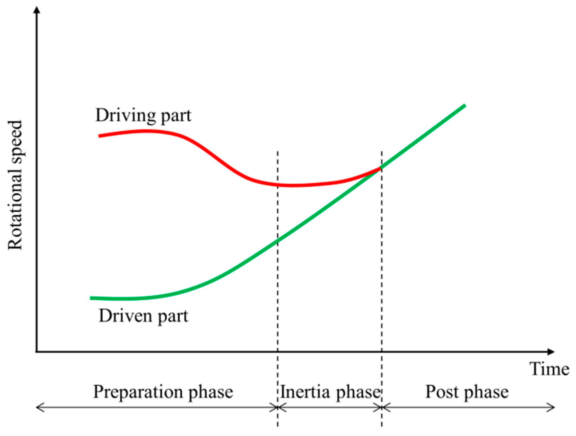
4.2. Control Principle

Given the above optimization objectives and the aforementioned constraints that are necessary for assuring the validation of the control-oriented continuous-time state space model and for guaranteeing the safe operation of the related components, the discrete-time model predictive control is suitable for this situation. The basic mechanism of the discrete-time model predictive control is that at each sampling instant, based on the measurement or estimation of the state vector and the control-oriented discrete-time state space model of the controlled object, the input vector at the current sampling instant can determine the output vector at the following sampling instant. Thus, for a prediction horizon, the trajectory of the input vector can determine the trajectory of the output vector. Because the control objective can be formulated as the cost function of the set-point trajectory and predicted trajectory of the output vector, within the prediction horizon, the trajectory minimizing the cost function and satisfying all the equality or inequality constraints is the optimum trajectory of the input vector. Because only the first sampling of the optimum trajectory is implemented as the input vector for the current sampling instant, the optimization process is repeated at the next sampling instant [26]. In terms of utilization in the mode transition control, the discrete-time model predictive control has two obvious advantages [27]. The first advantage is that the periodically updated optimum trajectory of the input vector can readily take the change of the driver’s torque demand into account. The second advantage is that the optimization process repeated at each sampling instant takes the powertrain’s actual state into account and can mitigate the influence of the model uncertainty.

4.3. Equilibrium State

In this paper, the definition of the term ‘equilibrium state’ is the hybrid powertrain state satisfying the sufficient and necessary ideal synchronization condition. Ideally, at the clutch engagement instant, the hybrid powertrain should reach the equilibrium state and consequently the responsiveness and smoothness of the propulsion torque exerted on the drivetrain by the hybrid power source are guaranteed. In accordance with Equation (26), the equilibrium state of the clutch sliding speed ${\omega }_{1eq}$ should be a positive value slightly larger than zero. This can guarantee the constraint (20) being satisfied against the influence of model uncertainty. Similarly, in accordance with Equation (28), the equilibrium state of the time derivative of torsion of the axle shaft ${\omega }_{2eq}$ should be chosen equal to zero. The equilibrium state of the engine output torque $M_{eeq}$ should be chosen equal to the engine output torque required by the energy management system of the hybrid powertrain $M_{eems}$. Similarly, the equilibrium state of the motor output torque $M_{meq}$ should be chosen equal to the motor output torque required by the energy management system of the hybrid powertrain $M_{mems}$. The equilibrium state of the torsion of the axle shaft ${\theta }_{eq}$ and the equilibrium state of the torque transmitted by the clutch $M_{ceq}$ can be calculated by:

$$\{\begin{array}{c}\frac{k}{J_2{i}_{fd}{\eta }_{fd}{i}_g{\eta }_g}{\theta }_{eq}-\left(\frac{1}{J_{epc}}+\frac{1}{J_2}\right)M_{ceq}=-\frac{1}{J_{epc}}{M}_{eeq}+\frac{1}{J_2}{M}_{meq}\\ -\left(\frac{k}{J_2{i}_{fd}^2{\eta }_{fd}{i}_g^2{\eta }_g}+\frac{k}{J_1}\right){\theta }_{eq}+\frac{1}{J_2{i}_{fd}{i}_g}{M}_{ceq}=-\frac{1}{J_2{i}_{fd}{i}_g}{M}_{meq}-\frac{1}{J_1}{M}_r\end{array}$$

(30)

Because only the first sampling of the optimum trajectory is implemented as the input vector for the current sampling instant and, in this paper, the sampling interval is ten milliseconds, the external resistance torque $M_r$ can be considered to be constant. The value of $M_r$ is computed by (17) at each sampling instant, and the control-oriented model of the hybrid powertrain is therefore updated at each sampling instant. The equilibrium state of the state vector of the control-oriented continuous-time state space model of the hybrid powertrain $\mathit{x}{\mathbf{1}}_{eq}$ can be formulated as:

$$\mathit{x}{\mathbf{1}}_{eq}={\left[\begin{array}{cccccc}{\omega }_{1eq}& {\theta }_{eq}& {\omega }_{2eq}& M_{eeq}& M_{ceq}& M_{meq}\end{array}\right]}^{\mathrm{T}}$$

(31)

The equilibrium state of the engine output torque command $M_{eceq}$ should be chosen equal to the equilibrium state of the engine output torque $M_{eeq}$. The engine time constant ${\tau }_e$ is approximately ten times as large as the clutch actuator time constant ${\tau }_c$ and approximately a hundred times as large as the motor time constant ${\tau }_m$. Thus, the engine responds to the torque command much slower than the clutch and motor. Given these engine output torque response characteristics, in this paper, the engine output torque command $M_{ec}$ is set equal to the equilibrium state of the engine output torque command $M_{eceq}$. The equilibrium state of the clutch torque command $M_{cceq}$ should be chosen equal to the equilibrium state of the torque transmitted by the clutch $M_{ceq}$. Similarly, the equilibrium of the motor output torque command $M_{mceq}$ should be chosen equal to the equilibrium state of the motor output torque $M_{meq}$. By introducing the equilibrium of the state vector and input vector, the control-oriented continuous-time state space model of CPPHP (23) can be refined as:

$$\dot{\mathit{x}}\mathbf{2}=\mathit{A}\mathbf{1}\mathit{x}\mathbf{2}+\mathit{B}\mathbf{1}\mathit{u}\mathbf{2}$$

(32)

with $\mathit{A}\mathbf{1}=\left[\begin{array}{cccccc}0& \frac{k}{J_2{i}_{fd}{\eta }_{fd}{i}_g{\eta }_g}& \frac{b}{J_2{i}_{fd}{\eta }_{fd}{i}_g{\eta }_g}& \frac{1}{J_{epc}}& -\left(\frac{1}{J_{epc}}+\frac{1}{J_2}\right)& -\frac{1}{J_2}\\ 0& 0& 1& 0& 0& 0\\ 0& -\left(\frac{k}{J_2{i}_{fd}^2{\eta }_{fd}{i}_g^2{\eta }_g}+\frac{k}{J_1}\right)& -\left(\frac{b}{J_2{i}_{fd}^2{\eta }_{fd}{i}_g^2{\eta }_g}+\frac{b}{J_1}\right)& 0& \frac{1}{J_2{i}_{fd}{i}_g}& \frac{1}{J_2{i}_{fd}{i}_g}\\ 0& 0& 0& -\frac{1}{{\tau }_e}& 0& 0\\ 0& 0& 0& 0& -\frac{1}{{\tau }_c}& 0\\ 0& 0& 0& 0& 0& -\frac{1}{{\tau }_m}\end{array}\right]$, $\mathit{B}\mathbf{1}=\left[\begin{array}{cc}0& 0\\ 0& 0\\ 0& 0\\ 0& 0\\ \frac{1}{{\tau }_c}& 0\\ 0& \frac{1}{{\tau }_m}\end{array}\right]$, $\mathit{x}\mathbf{2}=\mathit{x}\mathbf{1}-\mathit{x}{\mathbf{1}}_{eq}$ and $\mathit{u}\mathbf{2}={\left[\begin{array}{cc}{M}_{cc}-M_{cceq}& M_{mc}-M_{mceq}\end{array}\right]}^{\mathrm{T}}$.

4.4. Control-Oriented Discrete-Time State Space Model

The control-oriented discrete-time state space model is a prerequisite for the discrete-time model predictive controller design. Based on Equation (32), and in accordance with matrix methods for inhomogeneous systems, the control-oriented discrete-time state space model of the CPPHP can be formulated as:

$$\mathit{x}\mathbf{2}\left(k+1\right)=\mathit{A}\mathbf{2}\mathit{x}\mathbf{2}\left(k\right)+\mathit{B}\mathbf{2}\mathit{u}\mathbf{2}\left(k\right)$$

(33)

with $\mathit{A}\mathbf{2}=e^{\mathit{A}\mathbf{1}T}$ and $\mathit{B}\mathbf{2}={\int }_0^T{e}^{\mathit{A}\mathbf{1}t}dt\mathit{B}\mathbf{1}$. Where $\mathit{x}\mathbf{2}\left(k+1\right)$ denotes the state vector at sampling instant $k+1$, $\mathit{x}\mathbf{2}\left(k\right)$ the state vector at sampling instant $k$, $\mathit{u}\mathbf{2}\left(k\right)$ the input vector at sampling time $k$ and $T$ the sampling interval. Because shifting is inhibited during the mode transition, $\mathit{A}\mathbf{1}$ and $\mathit{B}\mathbf{1}$ are constant matrices during the mode transition. Thus, based on $\mathit{A}\mathbf{1}$ and $\mathit{B}\mathbf{1}$, $\mathit{A}\mathbf{2}$ and $\mathit{B}\mathbf{2}$ can be calculated by using the Matlab function ‘c2d’ with the specified sampling interval $T$.

4.5. Optimization Problem Formulation

Combining the responsiveness-related cost function $J_{c1}$ with the smoothness-related cost function $J_{c2}$, the optimization problem can be formulated as:

$$\text{Minimize} J_c={\displaystyle \sum _{i=1}^{N_p}}\mathit{y}{\left(k+i|k\right)}^{\mathrm{T}}\mathit{Q}\mathbf{1}\mathit{y}\left(k+i|k\right)+{\displaystyle \sum }_{i=0}^{N_p-1}\mathit{u}\mathbf{2}{\left(k+i|k\right)}^{\mathrm{T}}\mathit{R}\mathit{u}\mathbf{2}\left(k+i|k\right)$$

(34)

$$\text{Subject to} \mathit{c}\mathbf{1}\mathit{x}\mathbf{2}\left(k+1|k\right)\ge -\frac{1}{2}{\omega }_{1eq}\left(k\right)$$

(35)

$$\left[\begin{array}{c}-M_{cceq}\left(k\right)\\ M_{mcmin}-M_{mceq}\left(k\right)\end{array}\right]\le \mathit{u}\mathbf{2}\left(k|k\right)\le \left[\begin{array}{c}{M}_{ccmax}\left(k\right)-M_{cceq}\left(k\right)\\ M_{mcmax}-M_{mceq}\left(k\right)\end{array}\right]$$

(36)

with $\mathit{y}\left(k+i|k\right)=\mathit{C}\mathbf{1}\mathit{x}\mathbf{2}\left(k+i|k\right)$, $\mathit{C}\mathbf{1}=\left[\begin{array}{cccccc}1& 0& 0& 0& 0& 0\\ 0& 0& 1& 0& 0& 0\\ 0& 0& 0& 0& 1& 1\end{array}\right]$, $\mathit{Q}\mathbf{1}={\mathit{I}}_{3\times 3}$, $\mathit{R}=\left[\begin{array}{cc}{\mathit{R}}_{11}& 0\\ 0& {\mathit{R}}_{22}\end{array}\right]$ and $\mathit{c}\mathbf{1}=\left[\begin{array}{cccccc}1& 0& 0& 0& 0& 0\end{array}\right]$. Where $J_c$ denominates the cost function, $N_p$ the prediction horizon, $\mathit{y}\left(k+i|k\right)$ the predicted output vector for sampling instant $k+i$, $\mathit{Q}\mathbf{1}$ the weighting matrix for the output vector, $\mathit{u}\mathbf{2}\left(k+i|k\right)$ the chosen input vector for sampling instant $k+i$, $\mathit{R}$ the weighting matrix for the input vector, $\mathit{x}\mathbf{2}\left(k+1|k\right)$ the predicted state vector for sampling instant $k+1$, ${\omega }_{1eq}\left(k\right)$ the equilibrium state of the clutch sliding speed chosen at sampling instant $k$ and considered to be constant during the optimization process of sampling instant $k$, $M_{cceq}\left(k\right)$ the equilibrium state of the clutch torque command computed at sampling instant $k$ and considered to be constant during the optimization process of sampling instant $k$, $M_{ccmax}\left(k\right)$ the maximum allowable clutch torque command calculated at sampling instant $k$ in accordance with (21), $M_{mcmin}$ and $M_{mcmax}$ the minimum and maximum allowable motor output torque commands and $M_{mceq}\left(k\right)$ the equilibrium state of the motor output torque command computed at sampling instant $k$ and considered to be constant during the optimization process of sampling instant $k$. In accordance with the basic mechanism of the discrete-time model predictive control, only the first sampling of the optimum trajectory of the input vector is implemented, so only the constraints on the first sampling of the trajectory of the input vector have relatively major effects [26]. Thus the optimization problem formulation only includes constraints (35) and (36).

The cost function (34) can be refined as:

$$J_c={\displaystyle \sum _{i=1}^{N_p}}\mathit{x}\mathbf{2}{\left(k+i|k\right)}^{\mathrm{T}}\mathit{Q}\mathit{x}\mathbf{2}\left(k+i|k\right)+{\displaystyle \sum _{i=0}^{N_p-1}}\mathit{u}\mathbf{2}{\left(k+i|k\right)}^{\mathrm{T}}\mathit{R}\mathit{u}\mathbf{2}\left(k+i|k\right)$$

(37)

with $\mathit{Q}=\mathit{C}{\mathbf{1}}^{\mathrm{T}}\mathit{Q}\mathbf{1}\mathit{C}\mathbf{1}$.

The optimization problem can be simplified by introducing discrete-time Laguerre functions. The work presented in this paper is a prerequisite for an attempt to implement the designed discrete-time model predictive controller on an embedded micro control unit in future studies, so the computational load is sensitive. Theoretically, the number of parameters to be calculated directly influences the computational load of the optimization problem. The task of the discrete-time model predictive controller is solving the aforementioned optimization problem at each sampling instant. Solving the optimization problem is equivalent to finding the optimum trajectory of the input vector $\mathit{u}\mathbf{2}\left(k+i|k\right)$ for a specified prediction horizon $N_p$. Obviously, the number of parameters used to represent the trajectory increases rapidly with the increase of the prediction horizon $N_p$. Given that the duration of the mode transition is approximately one second and the sampling interval in this paper is ten milliseconds, the prediction horizon in this paper is set to be 100. Because this large prediction horizon is needed for high-performance, using discrete-time Laguerre functions can enormously decrease the number of parameters and consequently reduce the computational load. The discrete-time Laguerre functions can be formulated in a vector form as described in [26]:

$$\mathit{l}\left(k\right)={\left[\begin{array}{cccc}{l}_1\left(k\right)& l_2\left(k\right)& \dots & l_N\left(k\right)\end{array}\right]}^{\mathrm{T}}$$

(38)

$$\mathit{l}\left(k+1\right)={\mathit{A}}_l\mathit{l}\left(k\right)$$

(39)

with: ${\mathit{A}}_l=\left[\begin{array}{ccccc}a& 0& 0& \dots & 0\\ 1-a^2& a& 0& \dots & 0\\ \left(-a\right)\left(1-a^2\right)& 1-a^2& a& \dots & 0\\ \dots & \dots & \dots & \dots & \dots \\ {\left(-a\right)}^{N-2}\left(1-a^2\right)& {\left(-a\right)}^{N-3}\left(1-a^2\right)& {\left(-a\right)}^{N-4}\left(1-a^2\right)& \dots & a\end{array}\right]$ and $\mathit{l}\left(0\right)={\left[\begin{array}{cccc}\sqrt{1-a^2}& \sqrt{1-a^2}\left(-a\right)& \dots & \sqrt{1-a^2}{\left(-a\right)}^{N-1}\end{array}\right]}^{\mathrm{T}}$. Where $a\in \left[0,1\right)$ denotes the scaling factor and $N$ the number of discrete-time Laguerre functions. The inherent orthonormality of discrete-time Laguerre functions can be formulated as in [26]:

$${\displaystyle \sum _{k=0}^{\infty }}{l}_i\left(k\right)l_j\left(k\right)=\{\begin{array}{c}0, i\ne j\\ 1, i=j\end{array}$$

(40)

Due to the asymptotic stability of (39), discrete-time Laguerre functions can be used to represent the trajectory of the input vector and $\mathit{u}\mathbf{2}\left(k+i|k\right)$ can be formulated as:

$$\mathit{u}\mathbf{2}\left(k+i|k\right)=\left[\begin{array}{cc}\mathit{l}\mathbf{1}{\left(i\right)}^{\mathrm{T}}& \mathbf{0}\\ \mathbf{0}& \mathit{l}\mathbf{2}{\left(i\right)}^{\mathrm{T}}\end{array}\right]\mathit{\eta }$$

(41)

where $\mathit{l}\mathbf{1}\left(i\right)$ denominates the set of discrete-time Laguerre functions calculated in accordance with (38) and (39) with $a_1$ and $N_1$ as parameters, $\mathit{l}\mathbf{2}\left(i\right)$ the set of discrete-time Laguerre functions computed in accordance with (38) and (39) with $a_2$ and $N_2$ as parameters and $\mathit{\eta }$ a column vector with $N_1+N_2$ elements. In accordance with the control-oriented discrete-time state space model (33), the predicted state vector for sampling instant $k+i$ can be calculated by:

$$\mathit{x}\mathbf{2}\left(k+i|k\right)=\mathit{A}{\mathbf{2}}^i\mathit{x}\mathbf{2}\left(k\right)+{\displaystyle \sum _{j=0}^{i-1}}\mathit{A}{\mathbf{2}}^{i-1-j}\mathit{B}\mathbf{2}\mathit{u}\mathbf{2}\left(k+j|k\right)$$

(42)

Substituting (41) into (42), (42) can be refined further as:

$$\mathit{x}\mathbf{2}\left(k+i|k\right)=\mathit{A}{\mathbf{2}}^i\mathit{x}\mathbf{2}\left(k\right)+\mathit{\Phi }{\left(i\right)}^{\mathrm{T}}\mathit{\eta }$$

(43)

with $\mathit{\Phi }{\left(i\right)}^{\mathrm{T}}={\sum }_{j=0}^{i-1}\mathit{A}{\mathbf{2}}^{i-1-j}\mathit{B}\mathbf{2}\left[\begin{array}{cc}\mathit{l}\mathbf{1}{\left(j\right)}^{\mathrm{T}}& \mathbf{0}\\ \mathbf{0}& \mathit{l}\mathbf{2}{\left(j\right)}^{\mathrm{T}}\end{array}\right]$. Incorporating (43) into (37), the cost function (37) can be refined further as:

$$J_c={\displaystyle \sum _{i=1}^{N_p}}\mathit{x}\mathbf{2}{\left(k\right)}^{\mathrm{T}}{\left(\mathit{A}{\mathbf{2}}^i\right)}^{\mathrm{T}}\mathit{Q}\mathit{A}{\mathbf{2}}^i\mathit{x}\mathbf{2}\left(k\right)+{\mathit{\eta }}^{\mathrm{T}}\mathit{\Omega }\mathit{\eta }+2{\mathit{\eta }}^{\mathrm{T}}\mathit{\Psi }\mathit{x}\mathbf{2}\left(k\right)$$

(44)

with $\mathit{\Omega }={\sum }_{i=1}^{N_p}\mathit{\Phi }\left(i\right)\mathit{Q}\mathit{\Phi }{\left(i\right)}^{\mathrm{T}}+\left[\begin{array}{cc}{\mathit{R}}_{11}{\mathit{I}}_{N_1\times N_1}& \mathbf{0}\\ \mathbf{0}& {\mathit{R}}_{22}{\mathit{I}}_{N_2\times N_2}\end{array}\right]$ and $\mathit{\Psi }={\sum }_{i=1}^{N_p}\mathit{\Phi }\left(i\right)\mathit{Q}\mathit{A}{\mathbf{2}}^i$. The reformulation of the second term of (37) is based on the orthonormality of discrete-time Laguerre functions. Thus the aforementioned optimization problem can be reformulated as:

$$\text{Minimize} J_c={\mathit{\eta }}^{\mathrm{T}}\mathit{\Omega }\mathit{\eta }+2{\mathit{\eta }}^{\mathrm{T}}\mathit{\Psi }\mathit{x}\mathbf{2}\left(k\right)$$

(45)

$$\text{Subject to} \mathit{m}\mathbf{1}\mathit{\eta }\le {\gamma }_1$$

(46)

$$\mathit{M}\mathbf{1}\mathit{\eta }\le \mathit{\gamma }\mathbf{1}$$

(47)

$$\mathit{M}\mathbf{2}\mathit{\eta }\le \mathit{\gamma }\mathbf{2}$$

(48)

with $\mathit{m}\mathbf{1}=-\mathit{c}\mathbf{1}\mathit{B}\mathbf{2}\left[\begin{array}{cc}\mathit{l}\mathbf{1}{\left(0\right)}^{\mathrm{T}}& \mathbf{0}\\ \mathbf{0}& \mathit{l}\mathbf{2}{\left(0\right)}^{\mathrm{T}}\end{array}\right]$, ${\gamma }_1=\mathit{c}\mathbf{1}\mathit{A}\mathbf{2}\mathit{x}\mathbf{2}\left(k\right)+\frac{1}{2}{\omega }_{1eq}\left(k\right)$, $\mathit{M}\mathbf{1}=-\left[\begin{array}{cc}\mathit{l}\mathbf{1}{\left(0\right)}^{\mathrm{T}}& \mathbf{0}\\ \mathbf{0}& \mathit{l}\mathbf{2}{\left(0\right)}^{\mathrm{T}}\end{array}\right]$, $\mathit{\gamma }\mathbf{1}=\left[\begin{array}{c}{M}_{cceq}\left(k\right)\\ M_{mceq}\left(k\right)-M_{mcmin}\end{array}\right]$, $\mathit{M}\mathbf{2}=\left[\begin{array}{cc}\mathit{l}\mathbf{1}{\left(0\right)}^{\mathrm{T}}& \mathbf{0}\\ \mathbf{0}& \mathit{l}\mathbf{2}{\left(0\right)}^{\mathrm{T}}\end{array}\right]$ and $\mathit{\gamma }\mathbf{2}=\left[\begin{array}{c}{M}_{ccmax}\left(k\right)-M_{cceq}\left(k\right)\\ M_{mcmax}-M_{mceq}\left(k\right)\end{array}\right]$.

4.6. Optimization Solution

The control law of the discrete-time model predictive controller can be derived from the solution of the optimization problem. Essentially, this optimization problem is a quadratic programming problem. Similarly, the work presented in this paper is a prerequisite for an attempt to implement the designed discrete-time model predictive controller on an embedded micro control unit in future studies, so the convenience of programming and the existence of the solution are sensitive. Developing an explicit solution of the optimization problem can simplify the programming and guarantee the existence of the solution of the optimization problem. Due to the existence of inequality constraints, numerical methods for solving the quadratic programming problem need to identify inactive constraints and then ignore these constraints by introducing Lagrange multipliers. Obviously, $\mathit{m}\mathbf{1}$ and rows of $\mathit{M}\mathbf{1}$ and $\mathit{M}\mathbf{2}$ are not linearly independent, so there may be no solution for Lagrange multipliers. Introducing the ranking of constraints can solve this problem and reduce the computational load [26]. According to their importance, the constraints on the input vector have priority over that on the state vector because the former relates to the safe operation of the related components, whereas model uncertainty could interfere with the latter. Thus the inequality constraints (47) and (48) have a higher priority whereas the inequality constraint (46) has a lower priority. Taking the ranking of constraints into consideration, the procedure for solving the optimization problem can be formulated as the following:

• Solve the optimization problem without inequality constraints:

  $$\frac{d{J}_c}{d\mathit{\eta }}=0$$

  (49)

  $$\text{Then} \mathit{\eta }=-{\mathit{\Omega }}^{-1}\mathit{\Psi }\mathit{x}\mathbf{2}\left(k\right)$$

  (50)
• Check whether $\mathit{\eta }$ obtained in Step 1 satisfies the inequality constraint (46). If not, by introducing a Lagrange multiplier, compute $\mathit{\eta }$, the clutch torque command $M_{cc}\left(k\right)$ and the motor output torque command $M_{mc}\left(k\right)$:

  $$J_c={\mathit{\eta }}^{\mathrm{T}}\mathit{\Omega }\mathit{\eta }+2{\mathit{\eta }}^{\mathrm{T}}\mathit{\Psi }\mathit{x}\mathbf{2}\left(k\right)+\lambda \left(\mathit{m}\mathbf{1}\mathit{\eta }-{\gamma }_1\right)$$

  (51)

  $$\frac{\partial J_c}{\partial \mathit{\eta }}=\frac{\partial J_c}{\partial \lambda }=0$$

  (52)

  $$\text{Then} \lambda =-{\left(\mathit{m}\mathbf{1}{\left(2\mathit{\Omega }\right)}^{-1}\mathit{m}{\mathbf{1}}^{\mathrm{T}}\right)}^{-1}\left(\mathit{m}\mathbf{1}{\mathit{\Omega }}^{-1}\mathit{\Psi }\mathit{x}\mathbf{2}\left(k\right)+{\gamma }_1\right)$$

  (53)

  $$\mathit{\eta }=-{\left(2\mathit{\Omega }\right)}^{-1}\left(2\mathit{\Psi }\mathit{x}\mathbf{2}\left(k\right)+\mathit{m}{\mathbf{1}}^{\mathrm{T}}\lambda \right)$$

  (54)

  $$\mathit{u}\mathbf{2}\left(k|k\right)=\left[\begin{array}{cc}\mathit{l}\mathbf{1}{\left(0\right)}^{\mathrm{T}}& \mathbf{0}\\ \mathbf{0}& \mathit{l}\mathbf{2}{\left(0\right)}^{\mathrm{T}}\end{array}\right]\mathit{\eta }$$

  (55)

  $$\left[\begin{array}{c}{M}_{cc}\left(k\right)\\ M_{mc}\left(k\right)\end{array}\right]=\mathit{u}\mathbf{2}\left(k|k\right)+\left[\begin{array}{c}{M}_{cceq}\\ M_{mceq}\end{array}\right]$$

  (56)
• Check whether or not $\mathit{\eta }$ obtained in Step 2 satisfies the inequality constraints (47) and (48). If not, calculate the clutch torque command $M_{cc}\left(k\right)$ and the motor output torque command $M_{mc}\left(k\right)$:

  $$M_{cc}\left(k\right)=\{\begin{array}{c}0, \left[\begin{array}{cc}1& 0\end{array}\right]\left[\begin{array}{cc}\mathit{l}\mathbf{1}{\left(0\right)}^{\mathrm{T}}& \mathbf{0}\\ \mathbf{0}& \mathit{l}\mathbf{2}{\left(0\right)}^{\mathrm{T}}\end{array}\right]\mathit{\eta }<-M_{cceq}\left(k\right)\\ M_{ccmax}\left(k\right), \left[\begin{array}{cc}1& 0\end{array}\right]\left[\begin{array}{cc}\mathit{l}\mathbf{1}{\left(0\right)}^{\mathrm{T}}& \mathbf{0}\\ \mathbf{0}& \mathit{l}\mathbf{2}{\left(0\right)}^{\mathrm{T}}\end{array}\right]\mathit{\eta }>M_{ccmax}\left(k\right)-M_{cceq}\left(k\right)\end{array}$$

  (57)

  $$M_{mc}\left(k\right)=\{\begin{array}{c}{M}_{mcmin}, \left[\begin{array}{cc}0& 1\end{array}\right]\left[\begin{array}{cc}\mathit{l}\mathbf{1}{\left(0\right)}^{\mathrm{T}}& \mathbf{0}\\ \mathbf{0}& \mathit{l}\mathbf{2}{\left(0\right)}^{\mathrm{T}}\end{array}\right]\mathit{\eta }<M_{mcmin}-M_{mceq}\left(k\right)\\ M_{mcmax}, \left[\begin{array}{cc}0& 1\end{array}\right]\left[\begin{array}{cc}\mathit{l}\mathbf{1}{\left(0\right)}^{\mathrm{T}}& \mathbf{0}\\ \mathbf{0}& \mathit{l}\mathbf{2}{\left(0\right)}^{\mathrm{T}}\end{array}\right]\mathit{\eta }>M_{mcmax}-M_{mceq}\left(k\right)\end{array}$$

  (58)

Some parameters of the designed controller are given as the following: the equilibrium state of the clutch sliding speed ${\omega }_{1eq}$ is set to be 0.5 rad/s; the maximum motor output torque command $M_{mcmax}$ is set to be 50 Nm; and the minimum motor output torque command $M_{mcmin}$ is set to be −50 Nm.

The comparison of the computational times between the proposed quadratic programming solver and the Matlab standard quadratic programming solver ‘quadprog’ is shown in

Table 2. Comparison of the computational times.

Test	Proposed Solver	Quadprog (Interior-Point-Convex)	Quadprog (Active-Set)
1	0.030 ms	3.985 ms	1.221 ms
2	0.032 ms	3.989 ms	1.271 ms
3	0.031 ms	3.891 ms	1.228 ms
4	0.032 ms	3.913 ms	1.262 ms
5	0.033 ms	3.960 ms	1.251 ms

. The comparison of the obtained optimum solutions is shown in

Table 3. Comparison of the obtained optimum solutions.

Test	Proposed Solver	Quadprog (Interior-Point-Convex)	Quadprog (Active-Set)
1	$\left[\begin{array}{c}12.055\\ 42.717\end{array}\right]$	$\left[\begin{array}{c}12.055\\ 42.717\end{array}\right]$	$\left[\begin{array}{c}12.055\\ 42.717\end{array}\right]$
2	$\left[\begin{array}{c}12.055\\ 42.717\end{array}\right]$	$\left[\begin{array}{c}12.055\\ 42.717\end{array}\right]$	$\left[\begin{array}{c}12.055\\ 42.717\end{array}\right]$
3	$\left[\begin{array}{c}12.055\\ 42.717\end{array}\right]$	$\left[\begin{array}{c}12.055\\ 42.717\end{array}\right]$	$\left[\begin{array}{c}12.055\\ 42.717\end{array}\right]$
4	$\left[\begin{array}{c}12.055\\ 42.717\end{array}\right]$	$\left[\begin{array}{c}12.055\\ 42.717\end{array}\right]$	$\left[\begin{array}{c}12.055\\ 42.717\end{array}\right]$
5	$\left[\begin{array}{c}12.055\\ 42.717\end{array}\right]$	$\left[\begin{array}{c}12.055\\ 42.717\end{array}\right]$	$\left[\begin{array}{c}12.055\\ 42.717\end{array}\right]$

. The proposed solver and the Matlab standard solver provide identical optimum solutions.

The optimization problem to be solved is calculating the optimum input vector for the first sampling instant of the inertial phase and the values of the parameters in the solved quadratic programming problem are set equal to those chosen in Section 5. For each solver, the solving process is repeated five times for objectivity. The comparison is conducted in the Matlab programming environment in a laptop. The comparison in Table 2 and Table 3 shows the obvious advantages of the proposed quadratic programming solver in this paper.

5. Results and Discussion

5.1. Parameter Selection

The key parameters to be determined include $a_1$ and $N_1$ for generating discrete-time Laguerre functions used to represent the trajectory of the clutch torque command $M_{cc}$ and $a_2$ and $N_2$ for discrete-time Laguerre functions related to the trajectory of the motor output torque command $M_{mc}$. In accordance with (38) and (39), the scaling factor $a$ determines the rate of decay of discrete-time Laguerre functions and thereby the linear combination of these discrete-time Laguerre functions that is used to represent the trajectory of the input vector $\mathit{u}\mathbf{2}\left(k+i|k\right)$ in accordance with (41). Ideally, the clutch torque command $M_{cc}$ and the motor output torque command $M_{mc}$ should reach their respective equilibrium states simultaneously, so $a_1$ is chosen to be equal to $a_2$. Furthermore, for the sake of brevity, we choose $N_1$ to be equal to $N_2$. With respect to the cost function (37), choose the prediction horizon $N_p$ to be equal to infinity, and then the cost function can be formulated as:

$$J_c={\displaystyle \sum _{i=1}^{\infty }}\mathit{x}\mathbf{2}{\left(k+i|k\right)}^{\mathrm{T}}\mathit{Q}\mathit{x}\mathbf{2}\left(k+i|k\right)+{\displaystyle \sum _{i=0}^{\infty }}\mathit{u}\mathbf{2}{\left(k+i|k\right)}^{\mathrm{T}}\mathit{R}\mathit{u}\mathbf{2}\left(k+i|k\right)$$

(59)

The solution minimizing the cost function (59) is referred to as a discrete-time linear quadratic regulator. For arbitrary $a_1\in [0,1)$ and $a_2\in [0,1)$, as $N_1$ and $N_2$ increase, the optimum trajectory of the input vector obtained by minimizing the cost function (45) will converge to that obtained by minimizing the cost function (59) [26]. DLQR is not suitable to address the constraints, whereas DLQR is the ideal state feedback controller in the case of no constraints. DMPC is inherently adept at addressing the constraints. Thus, DLQR can be used to find reasonable parameters for the designed discrete-time model predictive controller and thereby the obtained DMPC can achieve high-performance similar to DLQR when the constraints become not active. The standard procedure for designing a discrete-time linear quadratic regulator is:

• Firstly, solve the following Riccati equation for finding the Riccati matrix ${\mathit{P}}_{\infty }$:

  $$\mathit{A}{\mathbf{2}}^{\mathrm{T}}\left({\mathit{P}}_{\infty }-{\mathit{P}}_{\infty }\mathit{B}\mathbf{2}{\left(\mathit{R}+\mathit{B}{\mathbf{2}}^{\mathrm{T}}{\mathit{P}}_{\infty }\mathit{B}\mathbf{2}\right)}^{-1}\mathit{B}{\mathbf{2}}^{\mathrm{T}}{\mathit{P}}_{\infty }\right)\mathit{A}\mathbf{2}+\mathit{Q}-{\mathit{P}}_{\infty }=0$$

  (60)
• Secondly, compute the state feedback gain matrix $\mathit{K}$:

  $$\mathit{K}={\left(\mathit{R}+\mathit{B}{\mathbf{2}}^{\mathrm{T}}{\mathit{P}}_{\infty }\mathit{B}\mathbf{2}\right)}^{-1}\mathit{B}{\mathbf{2}}^{\mathrm{T}}{\mathit{P}}_{\infty }\mathit{A}\mathbf{2}$$

  (61)
• Thirdly, calculate the optimum input vector for the current sampling instant:

  $$\mathit{u}\mathbf{2}\left(k|k\right)=-\mathit{K}\mathit{x}\mathbf{2}\left(k\right)$$

  (62)

Practically, the state feedback gain matrix $\mathit{K}$ can be computed by using the Matlab function ‘dlqr’ with the state matrix $\mathit{A}\mathbf{2}$, the input matrix $\mathit{B}\mathbf{2}$ and the weighting matrices $\mathit{Q}$ and $\mathit{R}$. In the case of $\mathit{Q}=\mathit{C}{\mathbf{1}}^{\mathrm{T}}\mathit{Q}\mathbf{1}\mathit{C}\mathbf{1}$ and $\mathit{R}={\mathit{I}}_{2\times 2}$, the effects of $a_1$, $a_2$, $N_1$ and $N_2$ on the difference between the optimum trajectory of the input vector determined by DMPC and that determined by DLQR are shown in Figure 6, Figure 7 and Figure 8.

These results demonstrate that for a given scaling factor, as $N_1$ and $N_2$ increase, the optimum trajectory calculated by DMPC converges to that computed by DLQR, and for given $N_1$ and $N_2$, too small or too large scaling factors result in the optimum trajectory calculated by DMPC deviating from that computed by DLQR. Based on these observations, comprehensively considering the need for accurately capturing the optimum trajectory determined by DLQR and the need for reducing the computational load, in this paper we choose $a_1=a_2=0.9$ and $N_1=N_2=5$.

The weighting matrix for the input vector $\mathit{R}$ is determined in the analysis of the performance of the designed discrete-time model predictive controller in the following section.

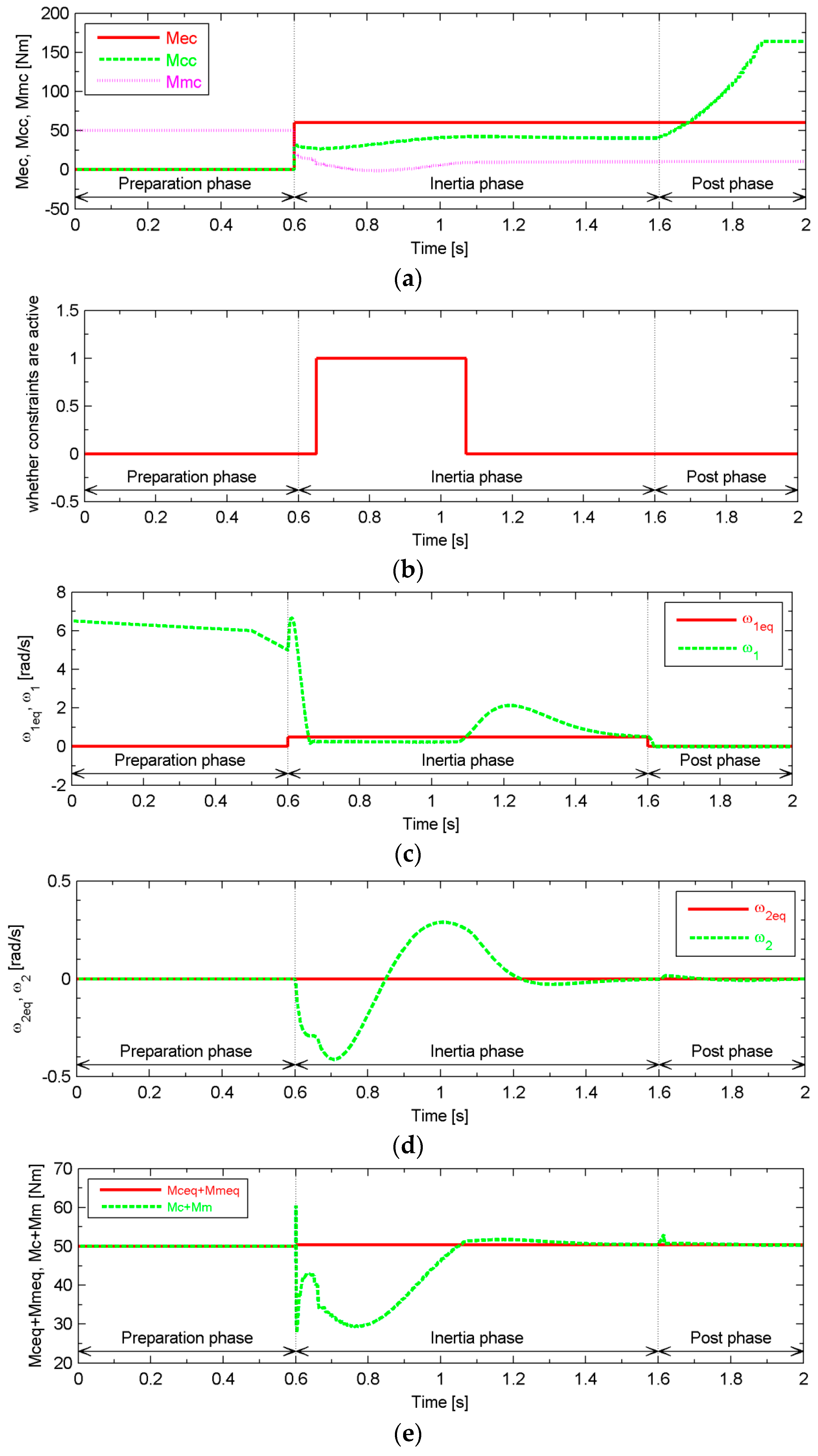
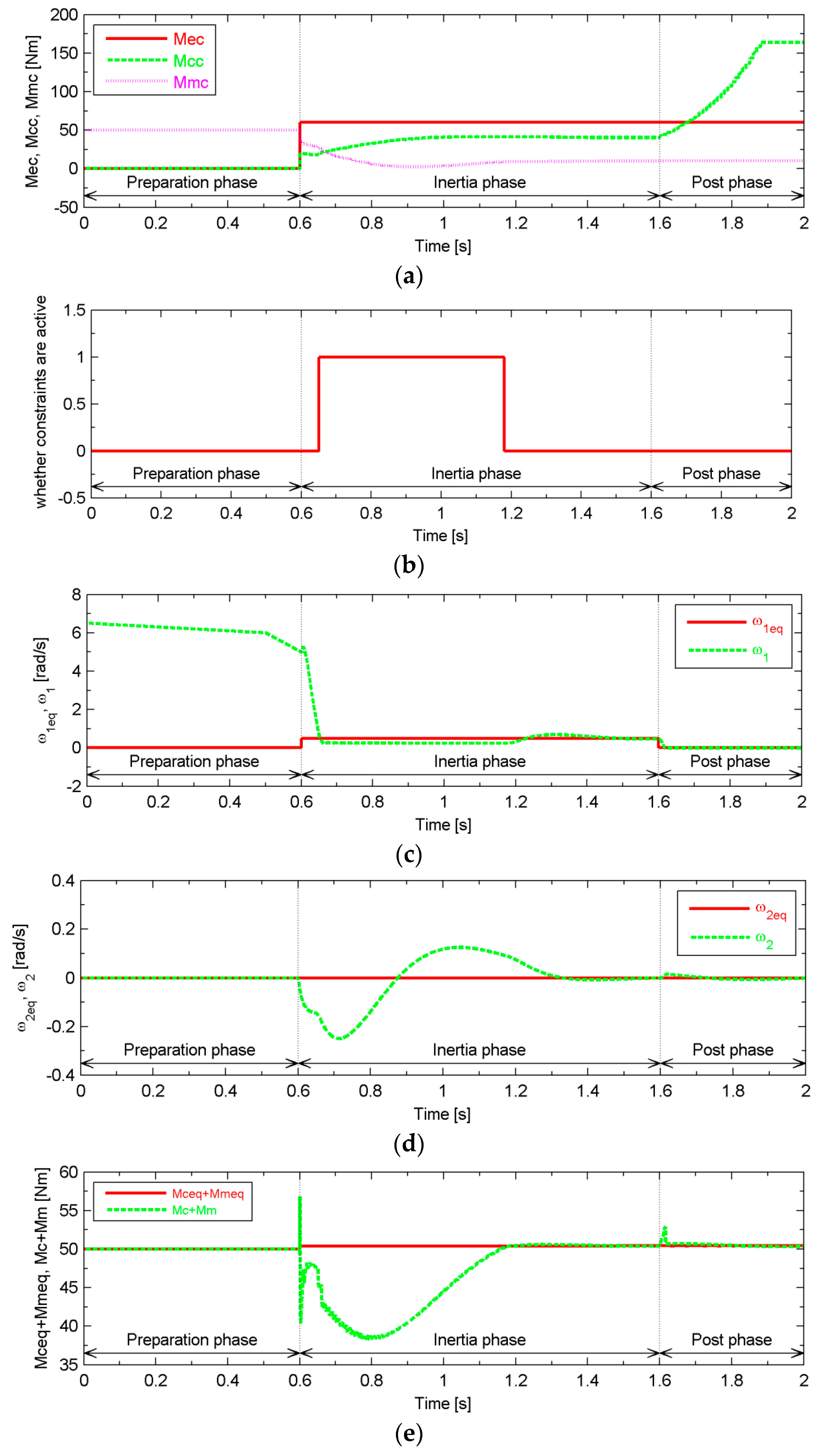
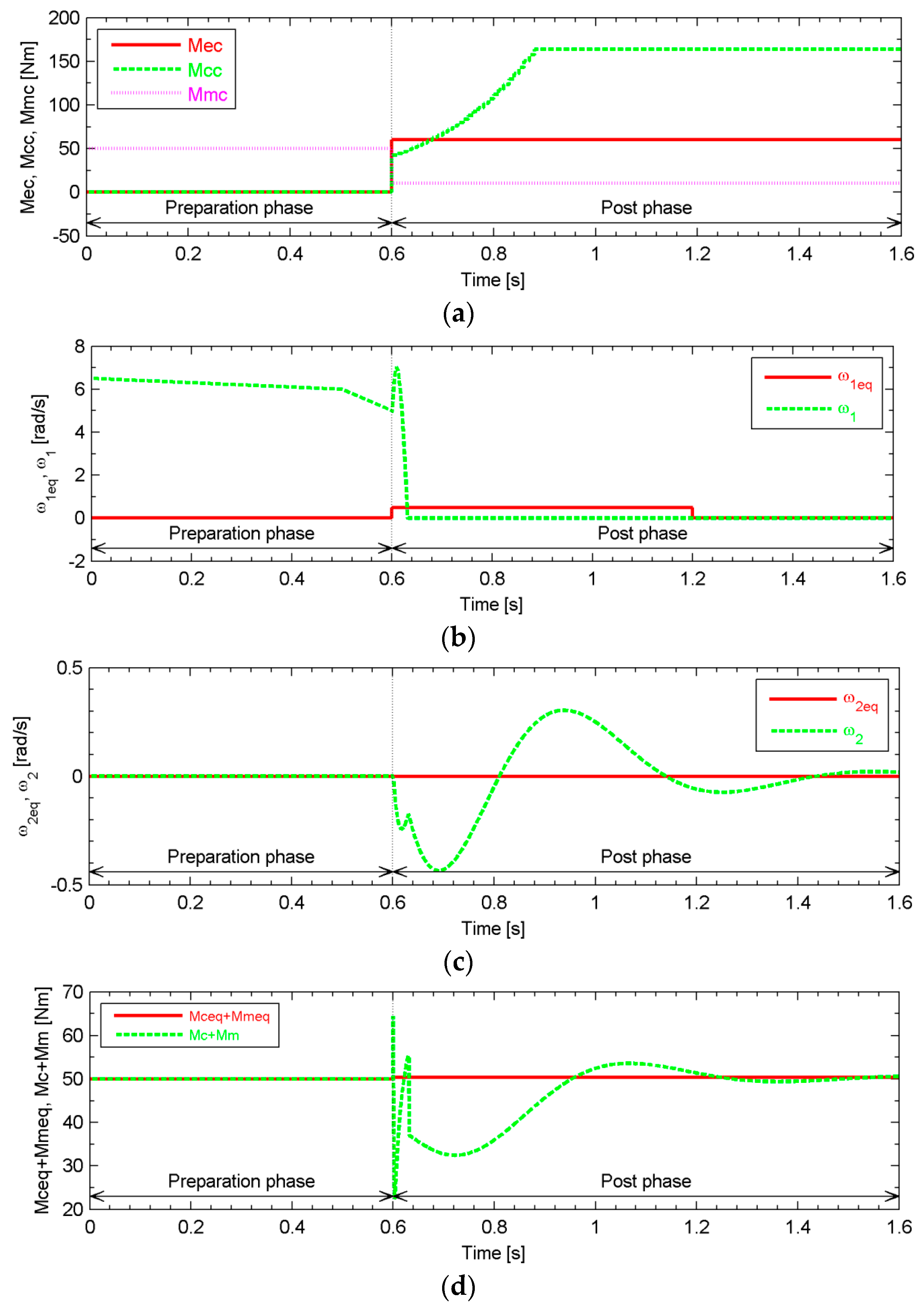
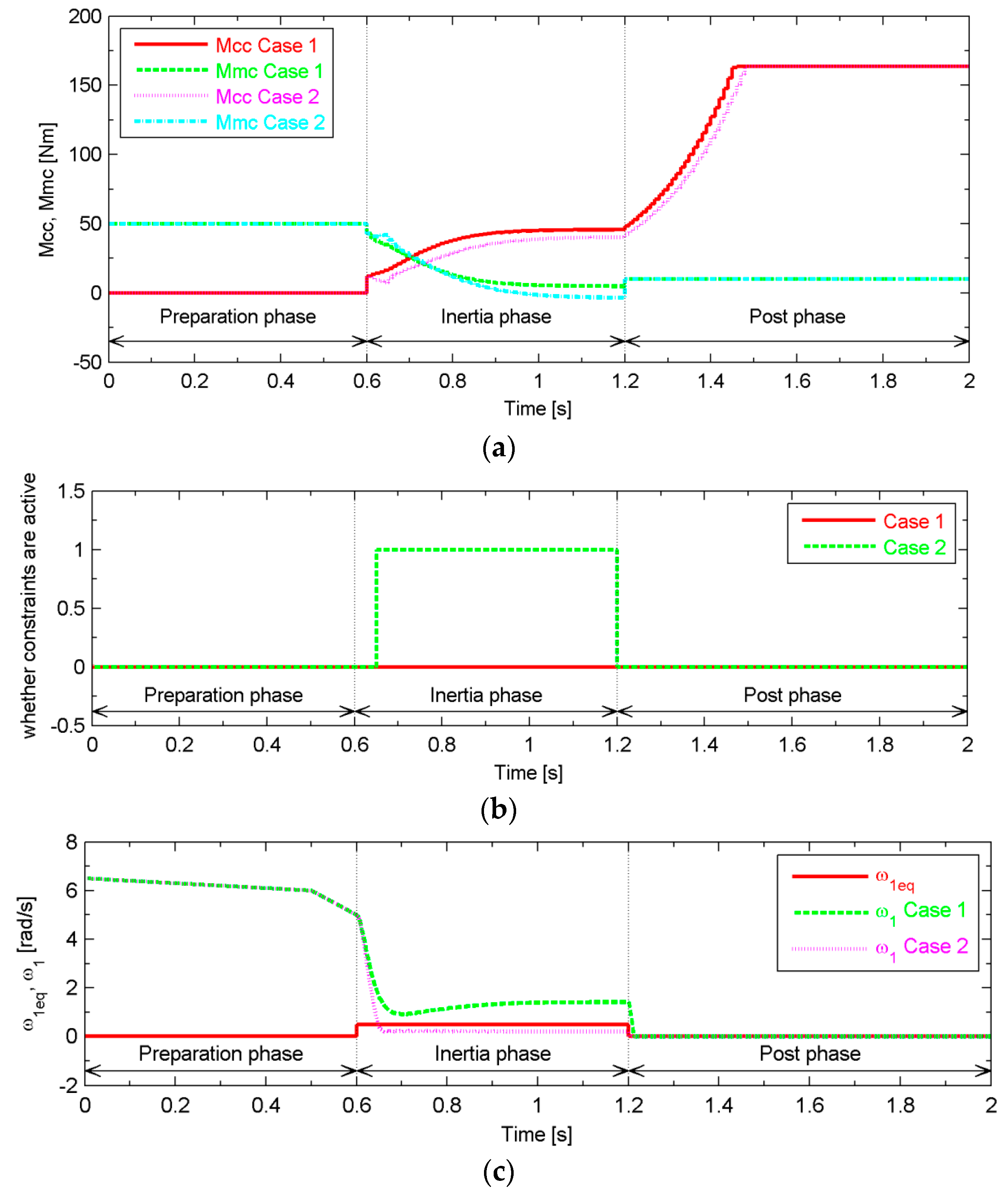
5.2. Performance in Nominal Conditions

The nominal conditions mean that the parameters used in the simulation-oriented model are identical with those used in the control-oriented model. The designed discrete-time model predictive controller originates from the control-oriented model. The scenario to be simulated is: firstly, the pre-transmission parallel hybrid powertrain operates in the pure electric propulsion mode; due to increase in the driver’s torque demand to address the extra resistance temporarily existing before and during the preparation phase, the energy management system claims that the hybrid powertrain should switch to the hybrid propulsion mode; thus, the engine is started and operates in the speed control mode, and the preparation phase begins; when the event that the engine speed falls into the specified range that is slightly larger than the motor speed triggers the designed discrete-time model predictive controller, the preparation phase ends and the inertia phase begins; the relevant state and input variables reaching their respective equilibrium states is the symbol of the ending of the inertia phase, and then the post phase begins; and the instant the post phase begins, the engine output torque command and the motor output torque command are set equal to their respective values required by the energy management system of the hybrid powertrain and the clutch torque command gradually increases to the maximum. The initial values of the relevant variables at the beginning of the inertia phase are shown in

Table 4. Initial values of the relevant variables.

Description	Symbol	Value
Initial engine output torque	$M_{e0}$	0 Nm
Initial rotational speed of $J_{epc}$	${\omega }_{epc0}$	285 rad/s
Initial normalized normal force	$r_{c0}$	0
Initial value of the average deflection of the bristles	$z_{c0}$	0 m
Initial motor output torque	$M_{m0}$	50 Nm
Initial rotational speed of $J_{cpmpp}$	${\omega }_{cpmpp0}$	280 rad/s
Initial wheel rotational speed	${\omega }_{w0}$	14 rad/s
Initial torsion of the axle shaft	${\theta }_0$	0.148 rad
Engine output torque required by the energy management system	$M_{eems}$	60 Nm
Motor output torque required by the energy management system	$M_{mems}$	10 Nm

.

The calculation results shown in Figure 9, Figure 10, Figure 11 and Figure 12 verify that for various combinations of weighting matrices the clutch torque command and the motor output torque command converge to their respective predefined equilibrium states simultaneously, and the clutch sliding speed and the time derivative of torsion of the axle shaft gradually tend toward their respective predefined equilibrium states. Given that the engine output torque command is set equal to the predefined equilibrium state during the mode transition and the external resistance torque can be considered to be constant during the sampling interval, the sufficient and necessary ideal synchronization condition has been satisfied, and thus the smoothness of the propulsion torque exerted on the drivetrain by the hybrid power source is validated. Additionally, the torque difference between the supplied by the hybrid power source and the demanded by the driver, shown in Figure 9, Figure 10, Figure 11 and Figure 12, demonstrates the high level of responsiveness of the propulsion torque exerted on the drivetrain by the hybrid power source. $M_{ceq}+M_{meq}$ denotes the torque demanded by the driver, and $M_c+M_m$ denominates the torque supplied by the hybrid power source. With respect to the duration of the mode transition, the convergence speed of relevant objects illustrated in Figure 9, Figure 10, Figure 11 and Figure 12 guarantees that the mode transition can be completed within an acceptable duration. The comparison of performance with different input vector weighting matrices confirms that the decrease of the input vector weighting matrix can augment the responsiveness and smoothness of the propulsion torque exerted on the drivetrain by the hybrid power source. However, when the input vector weighting matrix decreases to a relatively small level, the effects of any further decrease are limited because the chosen scaling factors compromise on accurately capturing the optimum trajectory determined by DLQR. Taking these observations into account, in this paper we choose $\mathit{R}=\left[\begin{array}{cc}0.01& 0\\ 0& 0.01\end{array}\right]$.

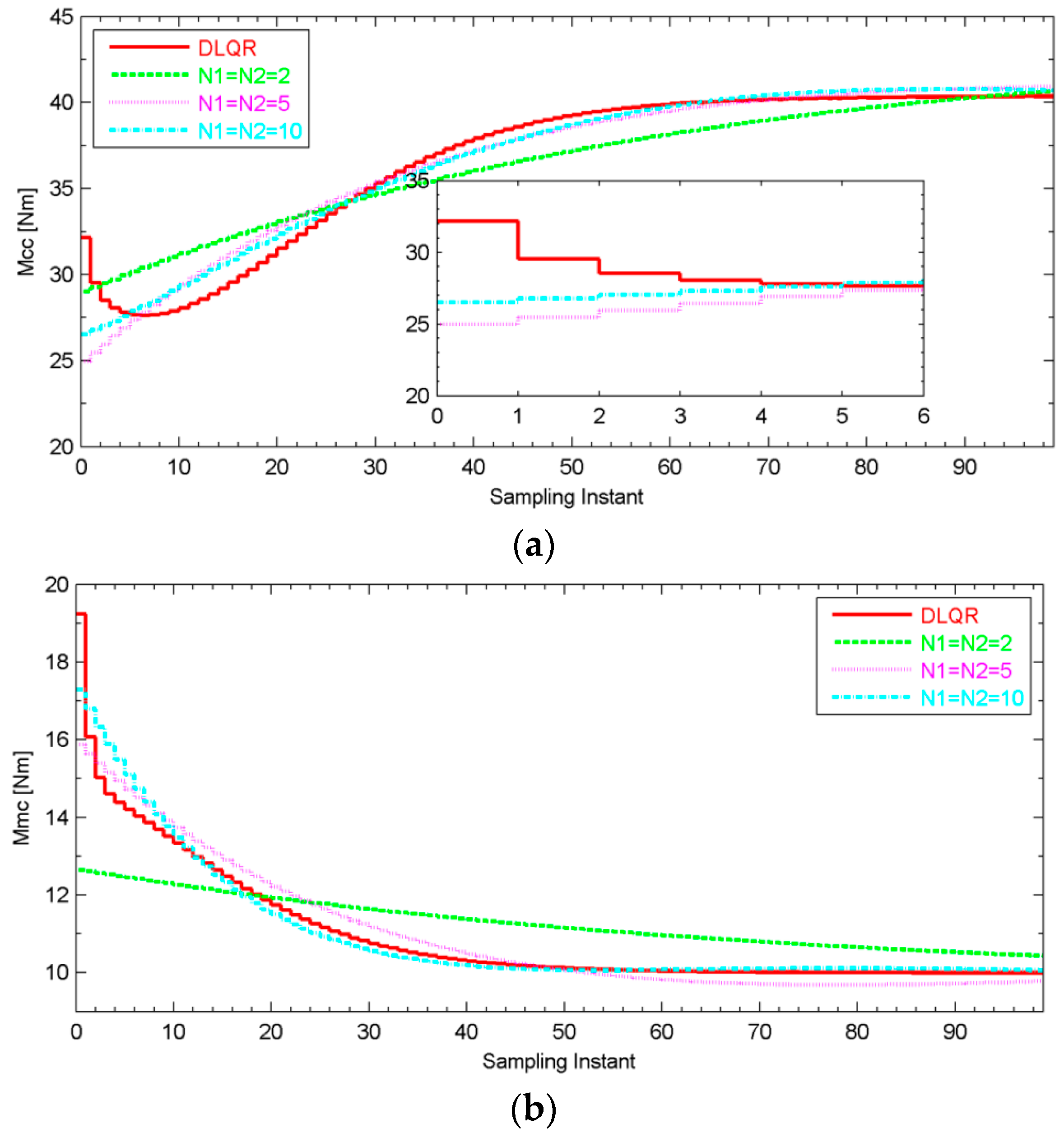
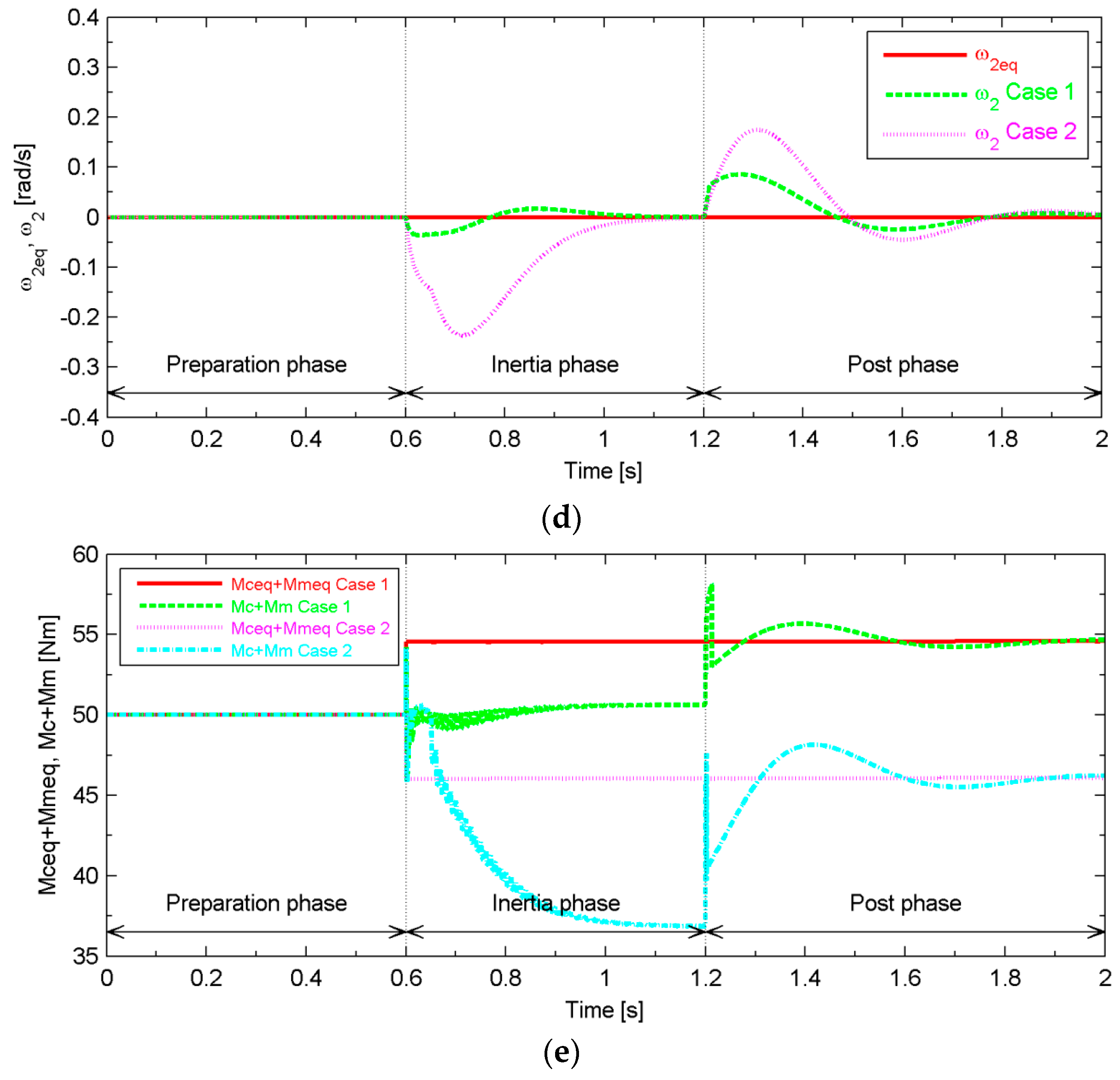
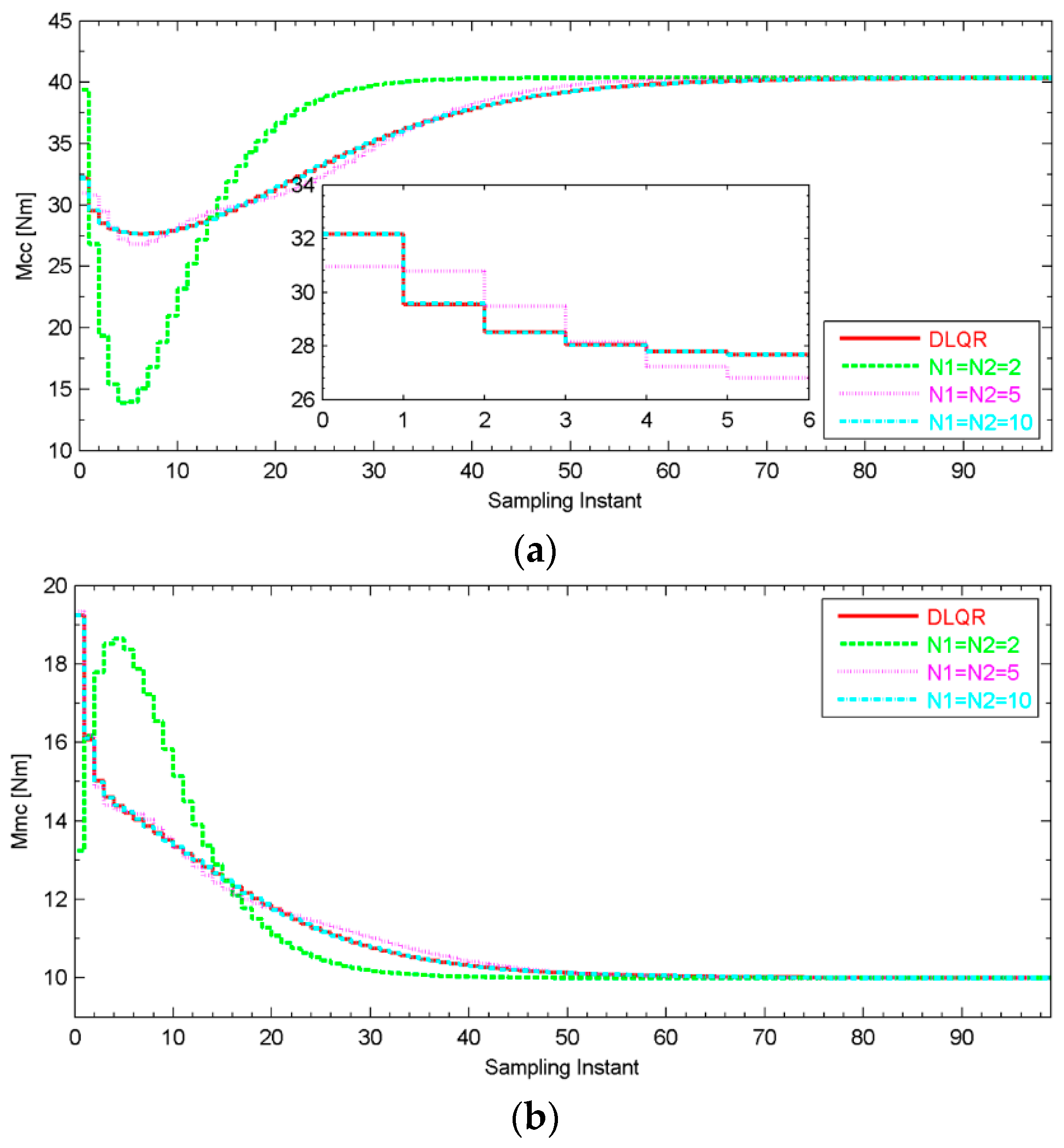
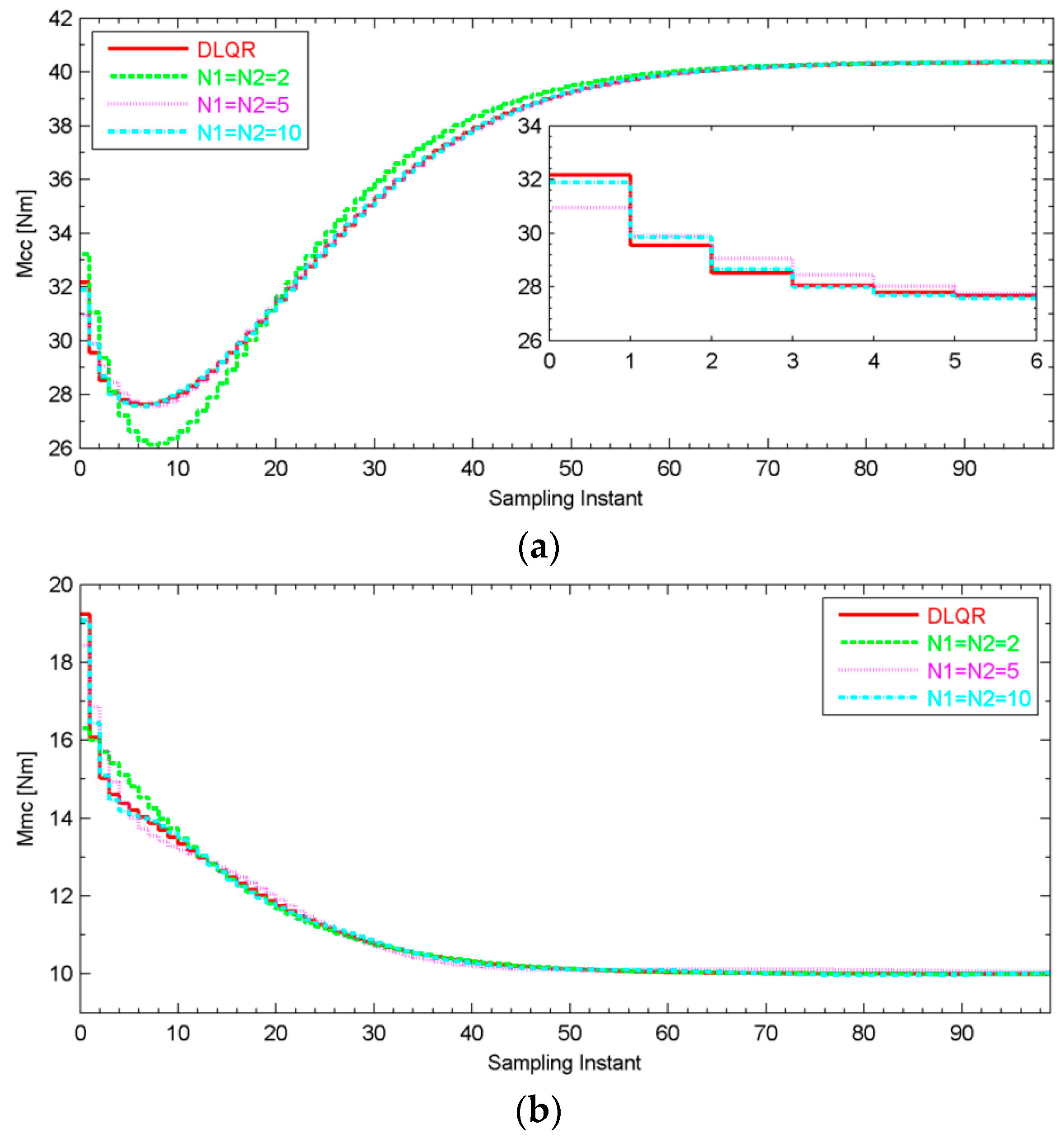
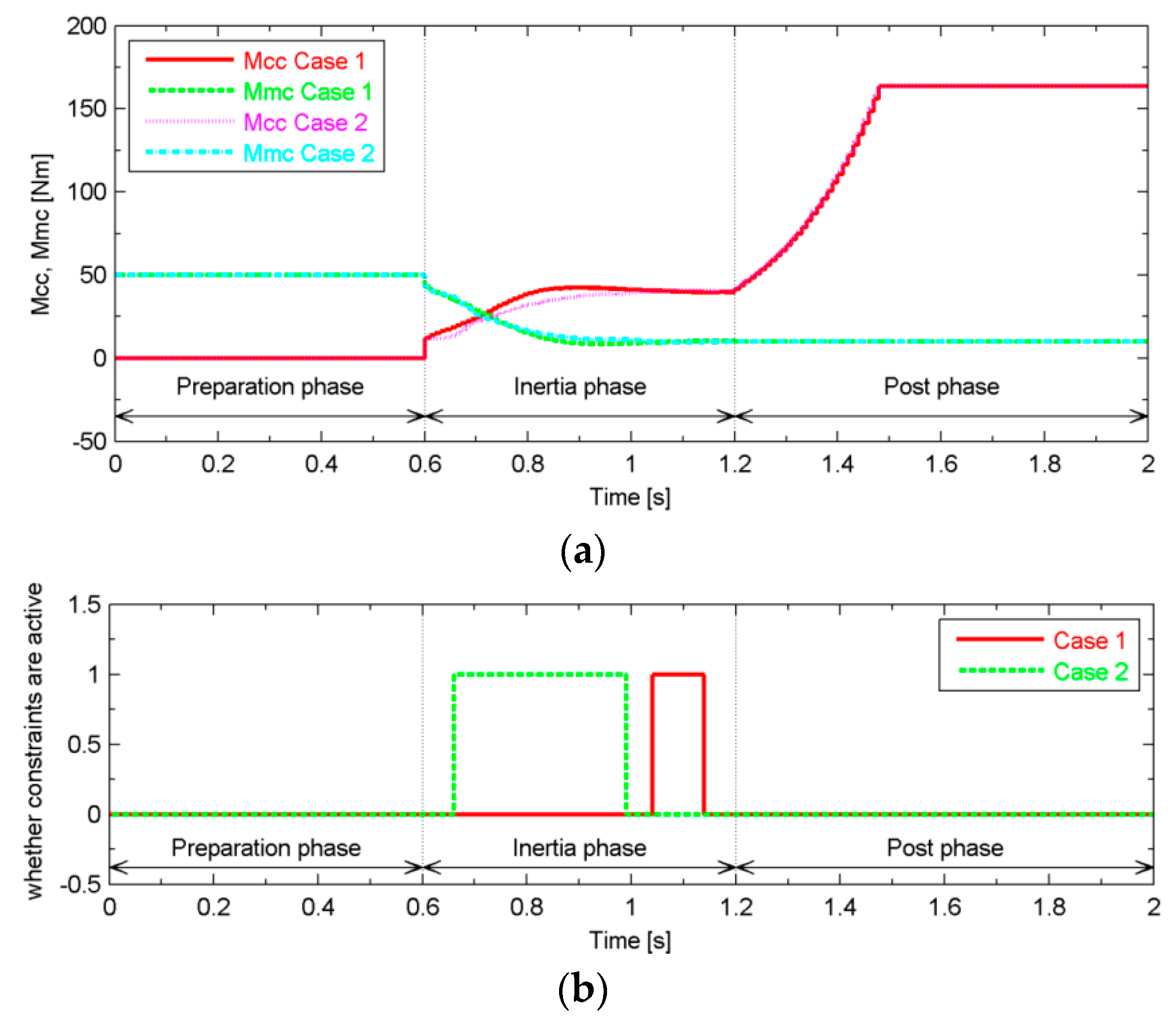
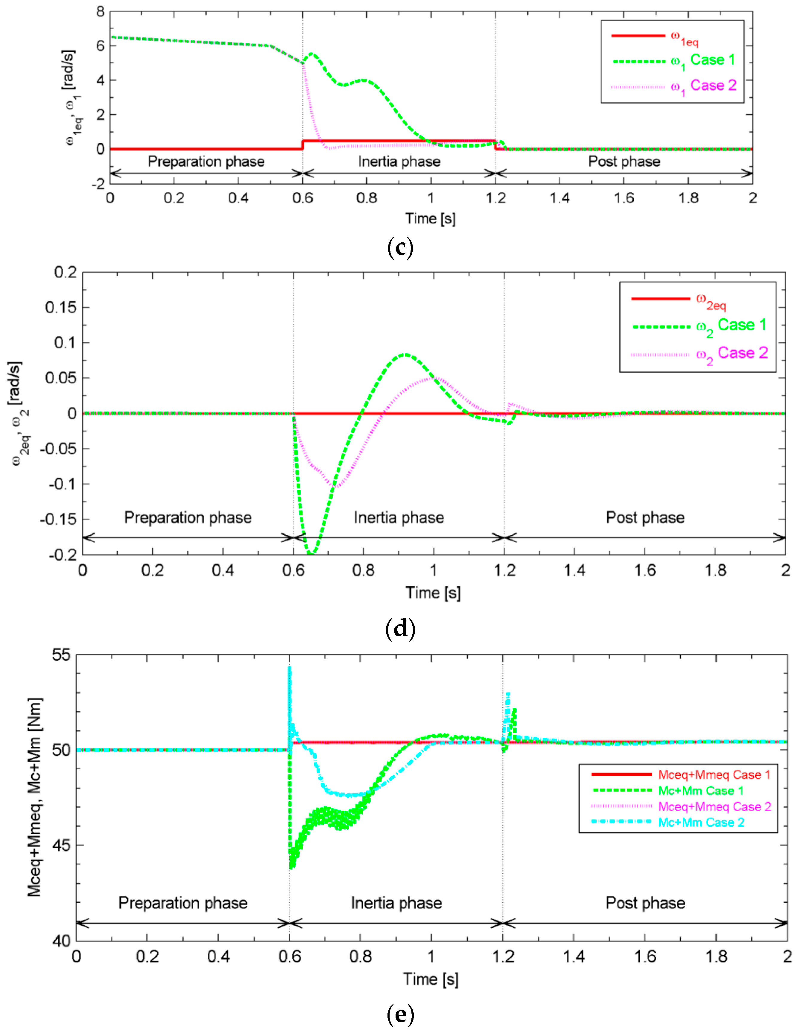
5.3. Comparison with Conditions Without DMPC

To validate the advantages of the designed discrete-time model predictive controller, the calculation results of the scenario without DMPC are shown in Figure 13. In this scenario, when the engine speed falls into the specified range that is slightly larger than the motor speed, the engine output torque command and the motor output torque command are set equal to the respective values required by the energy management system of the hybrid powertrain, and the clutch torque command gradually increases to the maximum in the same way that it changes in the scenario with DMPC.

Obviously, the torque difference between the supplied by the hybrid power source and the demanded by the driver in the scenario without DMPC is approximately ten times as large as that in the scenario adopting DMPC and the time derivative of torsion of the axle shaft in the scenario without DMPC is approximately six times as large as that in the scenario adopting DMPC.

5.4. Robustness

The designed discrete-time model predictive controller is based on the control-oriented model of the hybrid powertrain, and the control-oriented model may deviate from the actual system due to variations in the driving conditions and parameter uncertainty. Thus, the presented discrete-time model predictive controller should be robust to variations in the driving conditions and parameter uncertainty.

The calculation results shown in Figure 14 demonstrate the robustness of the designed controller in conditions different from the nominal conditions due to variations in the driving conditions. Clearly, during the mode transition, the steady states of the relevant state and input variables deviate from their respective predefined equilibrium values due to variations in the driving conditions. Still, during the mode transition, the designed controller guarantees that the clutch sliding speed and the time derivative of torsion of the axle shaft sustain steady states adjacent to their respective predefined equilibrium states, and the torque difference between the supplied by the hybrid power source and the demanded by the driver tends toward a steady level. Thus, the responsiveness and smoothness of the propulsion torque exerted on the drivetrain by the hybrid power source does not suffer from variations in the driving conditions. The calculation results shown in Figure 15 demonstrate the robustness of the designed controller in conditions different from the nominal conditions due to parameter uncertainty. Obviously, parameter uncertainty of the clutch actuator and motor time constants has almost no influence on the performance of the designed discrete-time model predictive controller. These calculation results indicate that the designed discrete-time model predictive controller is still stable in spite of variations in the driving conditions and parameter uncertainty, thereby validating the robustness of the designed controller.

6. Conclusions

In this paper, we propose a discrete-time model predictive controller applying to the mode transition from the pure electric propulsion mode to the hybrid propulsion mode in pre- transmission parallel hybrid electric vehicles. In the case of a long prediction horizon, due to the reformulation of the trajectory of the input vector by discrete-time Laguerre functions, the number of variables that needs to be computed is greatly reduced. By comparing the optimum trajectory of the input vector determined by DMPC with that determined by DLQR, which has the almost identical cost function with DMPC, the reasonable parameters are chosen. The calculation results demonstrate that the designed discrete-time model predictive controller can guarantee the responsiveness and smoothness of the propulsion torque exerted on the drivetrain by the hybrid power source during the mode transition, ensuring a high level of drivability. Additionally, the calculation results prove that the performance of the designed discrete-time model predictive controller does not suffer from variations in the driving conditions and parameter uncertainty. In future studies, the designed discrete-time model predictive controller will be refined further by deeply evaluating the importance of the introduced drivability-related indices and constraints in this paper.

References

1. Wu, G.; Zhang, X.; Dong, Z.M. Powertrain architectures of electrified vehicles: Review, classification and comparison. J. Franklin Inst. 2015, 352, 425–448. [Google Scholar] [CrossRef]
2. Qin, K.J.; Wang, E.H.; Zhao, H.; Shi, G.K.; Wang, R.G.; Kong, Z.G.; Wang, W. Development and experimental validation of a novel hybrid powertrain with dual planetary gear sets for transit bus applications. Sci. China Technol. Sci. 2015, 58, 2085–2096. [Google Scholar] [CrossRef]
3. Ouyang, M.G.; Zhang, W.L.; Wang, E.H.; Yang, F.Y.; Li, J.Q.; Li, Z.Y.; Yu, P.; Ye, X. Performance analysis of a novel coaxial power-split hybrid powertrain using a CNG engine and supercapacitors. Appl. Energy 2015, 157, 595–606. [Google Scholar] [CrossRef]
4. Fan, J.X.; Zhang, J.Y.; Shen, T.L. Map-Based power-split strategy design with predictive performance optimization for parallel hybrid electric vehicles. Energies 2015, 8, 9946–9968. [Google Scholar] [CrossRef]
5. Bishop, J.D.K.; Martin, N.P.D.; Boies, A.M. Cost-Effectiveness of alternative powertrains for reduced energy use and CO2 emissions in passenger vehicles. Appl. Energy 2014, 124, 44–61. [Google Scholar] [CrossRef]
6. Zou, Y.; Liu, T.; Sun, F.C.; Peng, H. Comparative Study of Dynamic Programming and Pontryagin’s Minimum Principle on Energy Management for a Parallel Hybrid Electric Vehicle. Energies 2013, 6, 2305–2318. [Google Scholar]
7. Nüesch, T.; Cerofolini, A.; Mancini, G.; Cavina, N.; Onder, C.; Guzzella, L. Equivalent Consumption Minimization Strategy for the Control of Real Driving NOx Emissions of a Diesel Hybrid Electric Vehicle. Energies 2014, 7, 3148–3178. [Google Scholar] [CrossRef]
8. Lakshmanan, S.; Palaniappan, A.; Chekuri, V. Methodology for Evaluation of Drivability Attributes in Commercial Vehicle; SAE Tech. Paper 2015-01-2767; SAE International: Warrendale, PA, USA, 2015. [Google Scholar]
9. Jayaraman, H.; Rao, N.; Muthiah, S.; Mohan, S. Optimization of Tip-In Response Character of Sports Utility Vehicle and Verification with Objective Methodology; SAE Tech. Paper 2015-01-1354; SAE International: Warrendale, PA, USA, 2015. [Google Scholar]
10. Khodabakhshian, M.; Feng, L.; Wikander, J. Optimization of Gear Shifting and Torque Split for Improved Fuel Efficiency and Drivability of HEVs; SAE Tech. Paper 2013-01-1461; SAE International: Warrendale, PA, USA, 2013. [Google Scholar]
11. Opila, D.F.; Aswani, D.; McGee, R.; Cook, J.A.; Grizzle, J.W. Incorporating drivability metrics into optimal energy management strategies for hybrid vehicles. In Proceedings of the 47th IEEE Conference on Decision and Control, Cancun, Mexico, 9–11 December 2008; pp. 4382–4389.
12. Opila, D.F.; Wang, X.Y.; McGee, R.; Gillespie, R.B.; Cook, J.A.; Grizzle, J.W. An energy management controller to optimally trade off fuel economy and drivability for hybrid vehicles. IEEE Trans. Control Syst. Technol. 2012, 20, 1490–1505. [Google Scholar] [CrossRef]
13. Koprubasi, K.; Westervelt, E.R.; Rizzoni, G. Toward the systematic design of controllers for smooth hybrid electric vehicle mode changes. In Proceedings of the 2007 American Control Conference, New York, NY, USA, 11–13 July 2007; pp. 2985–2990.
14. Kim, H.; Kim, J.; Lee, H. Mode transition control using disturbance compensation for a parallel hybrid electric vehicle. Proc. Inst. Mech. Eng. Part D J. Autom. Eng. 2010, 225, 150–166. [Google Scholar] [CrossRef]
15. Chen, L.; Xi, G.; Sun, J. Torque coordination control during mode transition for a series–parallel hybrid electric vehicle. IEEE Trans. Veh. Technol. 2012, 61, 2936–2949. [Google Scholar] [CrossRef]
16. Kum, D.; Peng, H.; Bucknor, N.K. Control of engine-starts for optimal drivability of parallel hybrid electric vehicles. J. Dyn. Syst. Meas. Control 2013, 135. [Google Scholar] [CrossRef]
17. Dolcini, P.; Canudas de Wit, C.; Béchart, H. Lurch avoidance strategy and its implementation in AMT vehicles. Mechatronics 2008, 18, 289–300. [Google Scholar] [CrossRef]
18. Walker, P.D.; Zhang, N. Active damping of transient vibration in dual clutch transmission equipped powertrains: A comparison of conventional and hybrid electric vehicles. Mech. Mach. Theory 2014, 77, 1–12. [Google Scholar] [CrossRef]
19. Lu, X.H.; Chen, H.; Gao, B.Z.; Zhang, Z.W.; Jin, W.W. Data-Driven predictive gearshift control for dual-clutch transmissions and FPGA implementation. IEEE Trans. Ind. Electron. 2015, 62, 599–610. [Google Scholar] [CrossRef]
20. Beck, R.; Saenger, S.; Richert, F.; Bolling, A.; Neiß, K.; Scholt, T.; Noreikat, K.E.; Abel, D. Model predictive control of a parallel hybrid vehicle drivetrain. In Proceedings of the 44th IEEE Conference on Decision and Control, and the European Control Conference, Seville, Spain, 12–15 December 2005; pp. 2670–2675.
21. Pisaturo, M.; Cirrincione, M.; Senatore, A. Multiple constrained MPC design for automotive dry clutch engagement. IEEE ASME Trans Mechatron 2015, 20, 469–480. [Google Scholar] [CrossRef]
22. Canudas de Wit, C.; Olsson, H.; Astrom, K.J.; Lischinsky, P. A new model for control of systems with friction. IEEE Trans. Autom. Control 1995, 40, 419–425. [Google Scholar] [CrossRef]
23. Gillespie, T.D. Fundamentals of Vehicle Dynamics; Society of Automotive Engineers (SAE) International: Warrendale, PA, USA, 1992. [Google Scholar]
24. Oh, J.J.; Choi, S.B.; Kim, J. Driveline modeling and estimation of individual clutch torque during gear shifts for dual clutch transmission. Mechatronics 2014, 24, 449–463. [Google Scholar] [CrossRef]
25. Van Berkel, K.; Hofman, T.; Serrarens, A.; Steinbuch, M. Fast and smooth clutch engagement control for dual-clutch transmissions. Control Eng. Pract. 2014, 22, 57–68. [Google Scholar] [CrossRef]
26. Wang, L.P. Model Predictive Control System Design and Implementation Using MATLAB; Springer-Verlag: London, UK, 2009. [Google Scholar]
27. Dolcini, P.J.; Canudas de Wit, C.; Béchart, H. Dry Clutch Control for Automotive Applications; Springer-Verlag: London, UK, 2010. [Google Scholar]
Figure 1. Typical hybrid powertrain architectures. (a) Typical planetary gear set based series-parallel hybrid powertrain configuration; (b) Typical clutch-based series-parallel hybrid powertrain configuration; (c) clutch-based pre-transmission parallel hybrid powertrain (CPPHP) configuration.
Energies 09 00740 g001
Figure 2. Process of clutch engagement.
Energies 09 00740 g002
Figure 3. Dynamics model of the CPPHP.
Energies 09 00740 g003
Figure 4. Matlab SimDriveline model of the CPPHP.
Energies 09 00740 g004
Figure 5. Comparison of the simulation results. (a) Comparison of the engine rotational speeds ω e p c and the motor rotational speeds ω c p m p p ; (b) Comparison of the vehicle longitudinal velocities v .
Energies 09 00740 g005
Figure 6. Difference between the optimum trajectories in the case of a 1 = a 2 = 0.8 . The sampling interval is ten milliseconds. (a) Difference between the optimum trajectories of the clutch torque command M c c ; (b) Difference between the optimum trajectories of the motor output torque command M m c .
Energies 09 00740 g006
Figure 7. Difference between the optimum trajectories in the case of a 1 = a 2 = 0.9 . The sampling interval is ten milliseconds. (a) Difference between the optimum trajectories of the clutch torque command M c c ; (b) Difference between the optimum trajectories of the motor output torque command M m c .
Energies 09 00740 g007
Figure 8. Difference between the optimum trajectories in the case of a 1 = a 2 = 0.99 . The sampling interval is ten milliseconds. (a) Difference between the optimum trajectories of the clutch torque command M c c ; (b) Difference between the optimum trajectories of the motor output torque command M m c .
Energies 09 00740 g008
Figure 9. Performance in nominal conditions with a 1 = a 2 = 0.9 , N 1 = N 2 = 5 , Q 1 = I 3 × 3 and R = I 2 × 2 . (a) Engine output torque command M e c , clutch torque command M c c and motor output torque command M m c ; (b) Conditions of the constraints; (c) Equilibrium state of the clutch sliding speed ω 1 e q and clutch sliding speed ω 1 ; (d) Equilibrium state of the time derivative of torsion of the axle shaft ω 2 e q and time derivative of torsion of the axle shaft ω 2 ; (e) Torque demanded by the driver M c e q + M m e q and torque supplied by the hybrid power source M c + M m .
Energies 09 00740 g009
Figure 10. Performance in nominal conditions with a 1 = a 2 = 0.9 , N 1 = N 2 = 5 , Q 1 = I 3 × 3 and R = [ 0.1 0 0 0.1 ] . (a) Engine output torque command M e c , clutch torque command M c c and motor output torque command M m c ; (b) Conditions of the constraints; (c) Equilibrium state of the clutch sliding speed ω 1 e q and clutch sliding speed ω 1 ; (d) Equilibrium state of the time derivative of torsion of the axle shaft ω 2 e q and time derivative of torsion of the axle shaft ω 2 ; (e) Torque demanded by the driver M c e q + M m e q and torque supplied by the hybrid power source M c + M m .
Energies 09 00740 g010
Figure 11. Performance in nominal conditions with a 1 = a 2 = 0.9 , N 1 = N 2 = 5 , Q 1 = I 3 × 3 and R = [ 0.01 0 0 0.01 ] . (a) Engine output torque command M e c , clutch torque command M c c and motor output torque command M m c ; (b) Conditions of the constraints; (c) Equilibrium state of the clutch sliding speed ω 1 e q and clutch sliding speed ω 1 ; (d) Equilibrium state of the time derivative of torsion of the axle shaft ω 2 e q and time derivative of torsion of the axle shaft ω 2 ; (e) Torque demanded by the driver M c e q + M m e q and torque supplied by the hybrid power source M c + M m .
Energies 09 00740 g011
Figure 12. Performance in nominal conditions with a 1 = a 2 = 0.9 , N 1 = N 2 = 5 , Q 1 = I 3 × 3 and R = [ 0.0001 0 0 0.0001 ] . (a) Engine output torque command M e c , clutch torque command M c c and motor output torque command M m c ; (b) Conditions of the constraints; (c) Equilibrium state of the clutch sliding speed ω 1 e q and clutch sliding speed ω 1 ; (d) Equilibrium state of the time derivative of torsion of the axle shaft ω 2 e q and time derivative of torsion of the axle shaft ω 2 ; (e) Torque demanded by the driver M c e q + M m e q and torque supplied by the hybrid power source M c + M m .
Energies 09 00740 g012
Figure 13. Scenario without DMPC. (a) Engine output torque command M e c , clutch torque command M c c and motor output torque command M m c ; (b) Equilibrium state of the clutch sliding speed ω 1 e q and clutch sliding speed ω 1 ; (c) Equilibrium state of the time derivative of torsion of the axle shaft ω 2 e q and time derivative of torsion of the axle shaft ω 2 ; (d) Torque demanded by the driver M c e q + M m e q and torque supplied by the hybrid power source M c + M m .
Energies 09 00740 g013
Figure 14. Performance in the case of variations in the driving conditions. Case 1: m = 1500   kg and α = 2 ° during the inertia phase and the post phase. Case 2: m = 1000 kg and α = 2 ° during the inertia phase and the post phase. Engine output torque command M e c steps from 0 Nm to 60 Nm at the beginning of the inertia phase. (a) Clutch torque command M c c and motor output torque command M m c ; (b) Conditions of the constraints; (c) Equilibrium state of the clutch sliding speed ω 1 e q and clutch sliding speed ω 1 ; (d) Equilibrium state of the time derivative of torsion of the axle shaft ω 2 e q and time derivative of torsion of the axle shaft ω 2 ; (e) Torque demanded by the driver M c e q + M m e q and torque supplied by the hybrid power source M c + M m .
Energies 09 00740 g014aEnergies 09 00740 g014b
Figure 15. Performance in the case of parameter uncertainty. Case 1: τ c = 0.05   s . Case 2: τ m = 0.005   s . Engine output torque command M e c steps from 0 Nm to 60 Nm at the beginning of the inertia phase. (a) Clutch torque command M c c and motor output torque command M m c ; (b) Conditions of the constraints; (c) Equilibrium state of the clutch sliding speed ω 1 e q and clutch sliding speed ω 1 ; (d) Equilibrium state of the time derivative of torsion of the axle shaft ω 2 e q and time derivative of torsion of the axle shaft ω 2 ; (e) Torque demanded by the driver M c e q + M m e q and torque supplied by the hybrid power source M c + M m .
Energies 09 00740 g015aEnergies 09 00740 g015b