Heuristic Methodology for Estimating the Liquid Biofuel Potential of a Region

Abstract

This paper presents a heuristic methodology for estimating the possible variation of the liquid biofuel potential of a region, an appraisal made for a future period of time. The determination of the liquid biofuel potential has been made up either on the account of an average (constant) yield of the energetic crops that were used, or on the account of a yield that varies depending on a known trend, which can be estimated through a certain method. The proposed methodology uses the variation of the yield of energetic crops over time in order to simulate a variation of the biofuel potential for a future ten year time period. This new approach to the problem of determining the liquid biofuel potential of a certain land area can be useful for investors, as it allows making a more realistic analysis of the investment risk and of the possibilities of recovering the investment. On the other hand, the presented methodology can be useful to the governmental administration in order to elaborate strategies and policies to ensure the necessity of fuels and liquid biofuels for transportation, in a certain area. Unlike current methods, which approach the problem of determining the liquid biofuel potential in a deterministic way, by using econometric methods, the proposed methodology uses heuristic reasoning schemes in order to reduce the great number of factors that actually influence the biofuel potential and which usually have unknown values.

1. Introduction

Contemporary societal development is closely related to existing energy sources based on fossil fuels (coal, oil and natural gas) [1,2]. However the technological development of human civilization has also had negative effects, among which we mention the most important ones: the generation of an intense pollution of the environment (with significant effects on the fauna, flora, and human health), but also an intense exploitation of fossil fuel reserves that has led to the situation of predicting their exhaustion in a relatively short time (several decades) [3,4,5].

The reaction that the human society has had to the issue of environmental pollution result in the adoption of a legislation which would ensure environment protection by all civilized states, and protocols and arrangements that are globally agreed (Rio de Janeiro-1992 and Kyoto-1997 [6]) by more and more states and stipulated terms and clear long-term objectives for reducing pollution.

The European Union (EU-27) has adopted and ratified the Kyoto Protocol [6], adopting rules and differentiated targets for each Member State [7]. Romania has to achieve the objective of reducing the emissions of greenhouse gases, mainly CO₂, with 27% by 2030, compared to the level of emissions in 1989.

This objective—which is applied with different values to all EU-27 member states—also led to a policy of supporting the implementation of renewable energy through incentives that would be offered to investors, mainly through the mechanism of green certificates.

Although switching to new energy sources has been performed erratically without a sufficiently accurate evaluation of the potential of each renewable energy sources, the overall effect would be beneficial if we take into account that sources of energy based on fossil fuels are going to be depleted in a short period of time—during the length of a generation—as specialists estimated.

An important consumer (and at the same time a major pollutant) is the transport sector—especially road transport—for which there are a large number of vehicles powered by combustion engines, based on fossil fuels (gasoline and diesel).

The depletion of fossil fuel deposits—especially the oil ones—will strongly affect the transport sector, even if engine manufacturers make sustained efforts to design and build engines that consume as little as possible. Because of this, finding an alternative to fossil fuels has become a stringent necessity and one of the options is represented by liquid biofuels.

Liquid biofuels are obtained from various agricultural plants by using various technological processes and are divided into two categories: bioethanol, alcohol-based fuel mix, possibly with gasoline, and biodiesel fuel which would be used in diesel engines, as a diesel equivalent. Due to the way the biofuels are obtained, they do not contain sulfur and a number of other pollutants present in fossil fuels, thus they are less polluting than classical gasoline and diesel fuel.

Replacing classic fuels (gasoline and diesel) with liquid biofuels raises a series of problems that need to be solved: the adaptation of engines in order to efficiently function with biofuels, the development of production technologies for biofuels from different raw materials, the establishment of economic effects and the influences on the environment generated by the introduction of biofuels, the establishment of ecologic balance which would allow the ensuring of food along with the development of cultures for biofuels.

The relevant literature covers a great number of issues, showing the interest of different groups of researchers for the replacement of fossil fuels with biofuels. In order to solve these problems important investments in production, storage and distribution equipment are required, investments which must be recovered and generate profit. By analyzing the causes for which several investments in renewable energy resources have failed in Romania, we concluded that most of these investments used estimations that were overly optimistic concerning the factors that can influence the investment, and they did not analyze correctly the potential risks. Because of this, the investors reached the situation in which they either could not finish the investment, or could not recover the invested money.

The causes of these errors can be found in the unrealistic presentation of the renewable energy resources, insisting on their positive aspects (inexistent or reduced emissions, reduced exploitation costs, the insurance of state support through the medium of green certificates etc.) and by neglecting the sensitive aspects if the investment (the dependence on climatic factors, the reduction of the agricultural areas that were used for obtaining food, the fluctuations of the fuel market, the fact that the state support can only be given for a limited period of time, etc.).

By analyzing the factors which can represent a risk for an investment in the liquid biofuel domain it was concluded that the climatic factor is the main element that could determine important variations of the bio-energetic crop production, which would mean variation of the liquid biofuel production.

In the literature, it could be remarked a lot of interest in replacing fossil fuels with biofuels for several groups of researchers. Therefore, in [8,9,10,11,12], there are presented estimations of the potentials of the renewable energy sources, at a global level. These estimations have been accomplished by using different methods, and they offer values of the potentials of renewable energy sources which have a high level of approximation.

The studies that discuss the biofuel resources at a global level [13,14,15,16] lead to estimations of the potentials of liquid or biomass biofuels which have the same high level of approximation. Also the approach of estimating the biofuel potential on a continental level [17,18,19,20,21,22] offers the same type of results, with approximate medium values and which contain information on the way the liquid biofuel potential varies due to the climatic factor.

There are also studies which approach this problem on a regional level—a country [23,24,25,26,27,28,29,30,31,32,33] or even a metropolitan zone [28]—but their results—despite having a higher precision level—do not contain data concerning the influence of the climatic factor.

Another category of literature concerns the technical and economic aspects on the production of biofuels that come from different resources [34,35,36,37,38]. These studies contain information concerning the yield and efficiency of the technological processes of obtaining biofuels from different crops [39,40,41,42,43] but do not offer data concerning the influence of the climatic factor on those crops.

Another aspect that is being approached in the literature regards the economic effects of implementing biofuels: the designing of supply and delivery chains for biofuels, the analysis of liquid fuel market, the optimization of field positioning the production plant [44,45,46,47], policies of supporting the usage of liquid biofuels [48], the efficiency of investments in the biofuel domain [49,50,51,52,53], etc.

The introduction of liquid biofuels on a large scale mainly means making a high volume of investments in plants production, but also in the logistics for transporting and storing them. As every investment needs pertinent information in order to ensure its recovery and the obtaining of a profit, the realistic estimation of liquid biofuels potential of a certain area becomes a problem of a great importance.

As it is argued in literature [29,30] the estimations of the biofuel potential that have been made at different levels (regional, global, local) were considered as average values, on the basis of simplifying hypotheses which cannot be applied in every area, so that the obtained results have a qualitative rather than a pragmatic characteristic. Even previsions designed for future intervals meant average values, which offered a view on the possibilities of covering the necessity of liquid fuels with biofuels. Because raw materials for biofuels are represented by the fruits or seeds of different crops, the production that could be obtained every year depends on a multitude of factors: climate and its periodic variations, diseases and pests, applied treatments, the type of cultivated plants, etc.

All these factors lead to annual variations of the production of every analyzed energetic crop. These variations are reflected in the level of liquid biofuel production and have implications that affect directly the incomes of the biofuel producers.

In this article, there is presented a methodology for forecasting the potential of biofuels for a certain region on a future time period ensuring that this potential would follow the variation of agricultural production which takes place in reality. It was considered that this approach is useful for investment projects in liquid biofuels—in order to evaluate as realistic as possible the risks of the investment—but also for the governmental administrations which therefore could elaborate strategies and realistic policies for implementing and supporting the production of liquid biofuels.

2. Methodological Considerations

The approach of this subject has started from the following observation: the biofuel potential of an area depends on the production volume of the crops production that are used for this purpose, and this production depends on a multitude of factors, as the climate is the most important one. Knowing that climatic factors present cyclic variations, it was considered as normal that these variations should be reflected both on the achieved production of the analyzed crops and on the achieved production of liquid biofuels.

The potential of energy sources based on biomass is estimated either globally through rough estimation of the production of various energy crops (wheat, corn, canola, sugar beet, potatoes, etc.) and the necessary for human consumption of each type, the difference representing the potential of biomass or particular level for a particular crop and a certain area—but also as an average value—obtained as the difference between the production in a given year and the human consumption.

The idea of analyzing the yield variations of the crops used as raw material for biofuels was inspired by data mining techniques. Data mining represents a large group of algorithms and methods to analyze large data volumes and to extract behavioral patterns for that data [54]. Usually data mining needs large volumes of data but in that analysis we try to use heuristic reasoning schemas and supplementary information about the problem for extracting a pattern of crops yield variations. As a further step in the research are presented considerations that have been the basis for elaborating the methodology to determine the liquid biofuels potential of a region.

The production of crops that can be used for liquid biofuel (wheat, corn, other cereals, potatoes, sugar beet, rapeseed, sunflower, and soybean) is typically used for other purposes too, such as: human and animal nutrition, industry, etc., thus restricting the availability for biofuels.

The land area which is annually cultivated with a specific crop depends on economic conditions of the market for that crop (a too low price per kg or ton, in a year, can lead to a strong reduction of cultivated land area in the next year) as well as the soil condition (soil protection requires regular crop rotation to avoid exhaustion thereof). The economic conditions of the market represent a subjective factor that cannot be quantified precisely, along with the pedological factors, which is an objective factor but it cannot be also quantified precisely.

Considering as constant the land area which is cultivated with a specific culture for biofuel crops the cycling variations of the yield will induce variations of the potential of biofuel. Knowing these variations will allow a more realistic planning of investments in this area and the real possibility to recover such investments. Also knowing the variation of the potential of biofuel for each crop there may be adopted reorganization strategies of crops in order to provide the necessary of biofuel for the transport sector every year.

The potential of liquid biofuels depends every year on the production that is obtained that year from each used crop, but the factor that determines that certain production depends on the yield of each analyzed culture as this yield is influenced by several factors, such as:

• The specific climate of the analyzed area;
• The climate evolution in the analyzed area;
• The climate evolution during a crop year;
• The land type;
• The cultivated land area;
• The production per hectare (yield);
• The crop system (irrigated or non-irrigated);
• The application or not of phytosanitary treatments;
• The usage or not of fertilizers and their type;
• The frequency of crop rotation;
• The processing technology used;
• Other factors with relatively low influence that cannot be quantified.

The large number of factors influencing the yield of crops and the production obtained within a year of that culture makes it practically impossible to achieve a deterministic mathematical model which would include all these influence factors that allow the making of a realistic assessment of the potential production of crops for the biofuel production. For this reason it was preferred to searching for a heuristic method to address this problem.

A heuristic method [55] is a query method that does not rely on a precise mathematical method and the operations performed were not purely deterministic. It does not give an accurate result for a certain problem, but can provide a result that meets best initial requirements of the problem. Generally, a heuristic method is used when the analyzed problem does not have a deterministic method to be solved. The methodology which has been proposed starts from the following assumptions:

• The potential of a region for producing liquid biofuels is directly proportional with the production of bioenergy crops;
• The production of a bioenergy crop is directly proportional to the cultivated land area and with the yield of that crop;
• Due to the fact that the number of factors which could influence the yield of a crops is high and these factors are correlated and can influence one another in ways that are hard to quantify, we considered that the yield of a bioenergy crop reflects the influence of all those factors in a certain year.

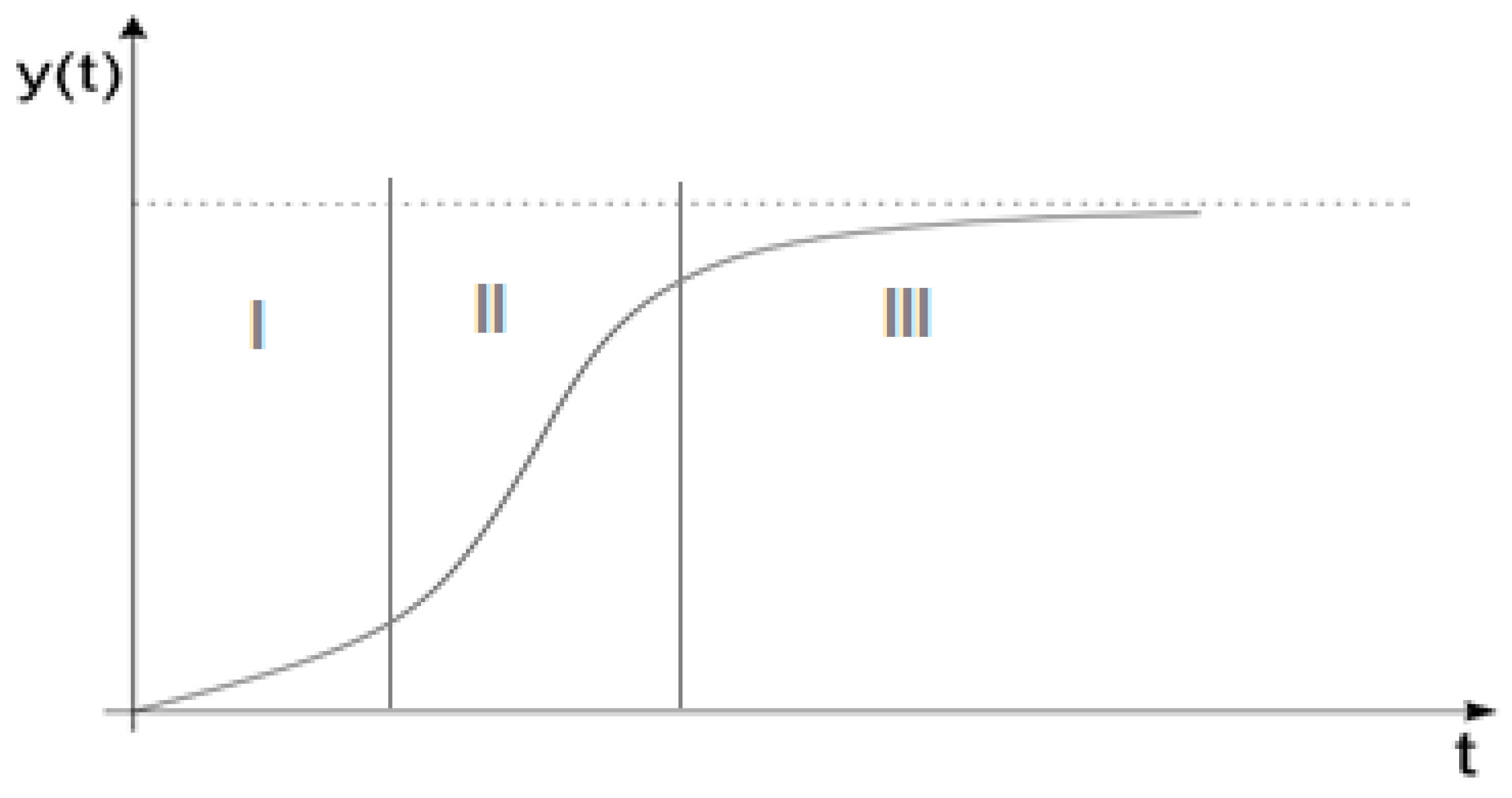
From a theoretical perspective, the yield of a culture evolves asymptotically to a maximum value, which cannot be overcome due to objective causes, which are imposed by the biological limits of the cultivated crop (crop yield cannot increase endlessly, regardless of how much fertilizer we provide or how densely we plant the respective crop, etc.). It results that the yield evolution of a crop is similar to the logistics curve (as it can be seen in the Figure 1).

In Figure 2, it is shown that this assumption is confirmed for France and Italy and for grain yield (in fact for many other countries, but all the results are not shown in order to not unnecessarily clutter the graph).

Further the aspects presented above will be used in order to determine the technical potential of liquid biofuels for a region because this potential is very important for investment planning and for estimating afferent risks. The great variations of the yield of the crops will lead to great variations of the liquid biofuels’ potential and will have the greater influence on the economic yield of an investment in liquid biofuels (generally Net Present Value and Internal Rate of Return are determined considering the yield of the crops to be constant, as its variations make the estimations imprecise).

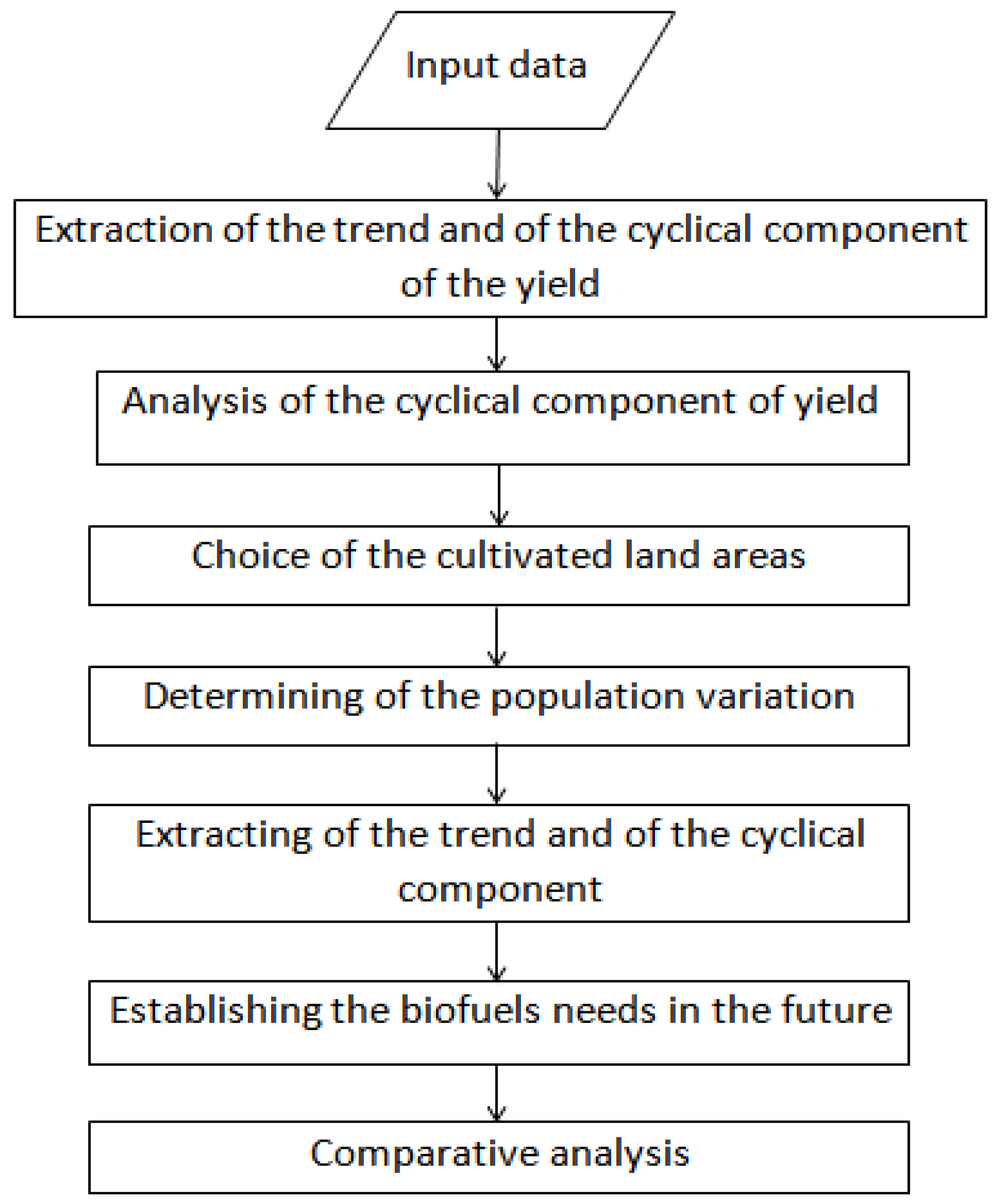
3. The Methodology for Estimating Variation of Liquid Biofuels Potential

The methodology that is proposed in this research is presented in the next flow-chart (Figure 3).

The input data for this methodology is represented by the yield values of every analyzed bio-energetic crop. This data is staggered over a long period of time—as long as possible—along with the values of the land area that is being cultivated with these crops and with the values for human/animal consumption and for industrial needs:

Step 1. Extraction of the Trend and Cyclical Component of the Yield of the Analyzed Crops.

The yield of a crop, analyzed during a certain longer period of time—tens of years—can be considered as a time series with two components: the trend and the cyclical component. A time series of classical period of time is a function that describes the variation of the sizes depending on the time at which the value of that size was measured.

A time series consists of three components [57], y_i = t_i + s_i + c_i, where:

• Trend t_i is the tendency of that size variation;
• Seasonal component s_i, that keeps the respective size variation throughout the year (tucked number of tourists visiting some sightseeing etc.);
• Cyclical component c_i that is a periodic variation of the analyzed size which has a period of time measured in years. The cyclical component can be regular, with a constant variation period or it may have irregular periodicity which most often will still falls within certain limits.

Taking into account that the values analyzed in this paper are represented by the crop yields—which is determined for a calendar year—we cannot speak about seasonality and only about cyclicity and the cyclical component that can be obtained by the following relationship if there is known the trend of the respective time series: c_i = y_i − t_i.

Through the medium of the proposed methodology, the extraction of the cyclic component from the variation of the yield of a crop was followed —on a period of time as long as possible—the analysis of this component and the extraction of a cycle that can be considered suitable for the worst case scenario in order to plan an investment. In the end this cycle of variation will be used in order to forecast the evolution of the yield of that certain culture for a future time period $y_j^F= t_j+c_j$ where $y_j^F$ is the future yield in the year j; t_j is the trend of yield in the year j (could be constant or can respect a specific variation law) and c_j is the cyclic component of yield established for the year j.

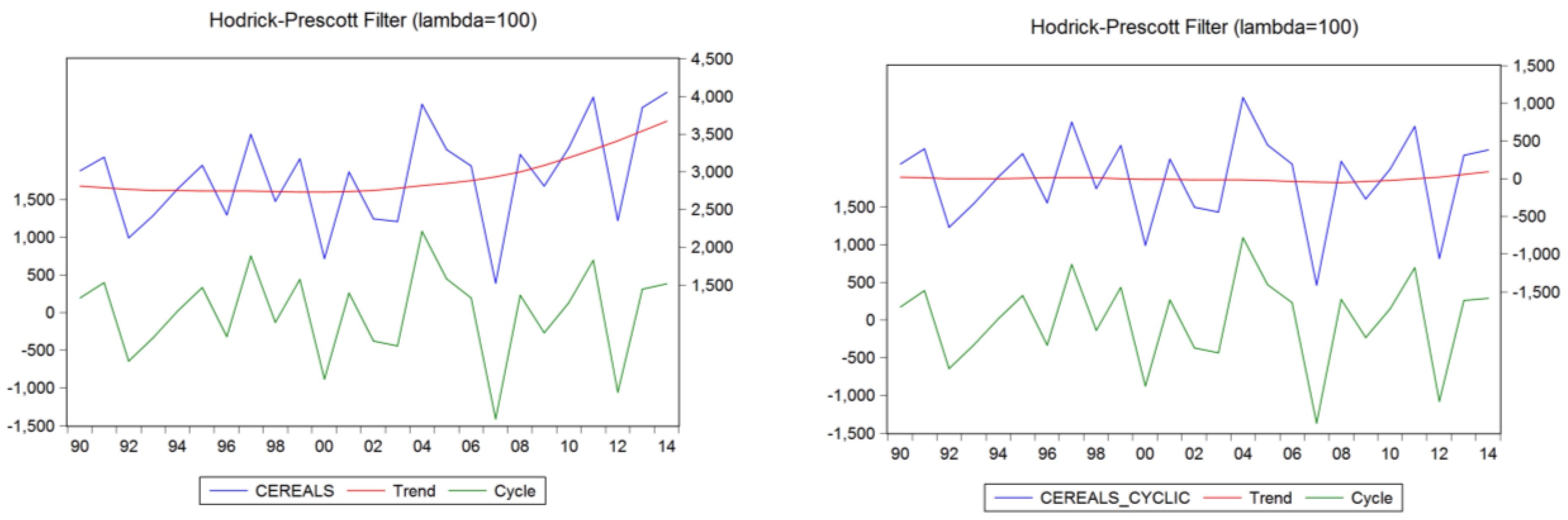
To determine the trend of the time series of the yield has been used the Hodrick-Prescott filter [58,59] (processing data in Eview). The Hodrick-Prescott filter is a standard technique used in macroeconomics for decomposing time series data into its trend and cyclical components. It is recognized as a common place tool used in macroeconomics and it was implemented in many software applications like: Matlab, Eviews, etc.

To verify the solution for this trend the following heuristic criterion has been used: if the determined trend coincides with the real trend of initial time series then the series represented by the cyclical component will have a constant trend (the graphic representation of the trend of cyclical component will be horizontal or very close to this position).

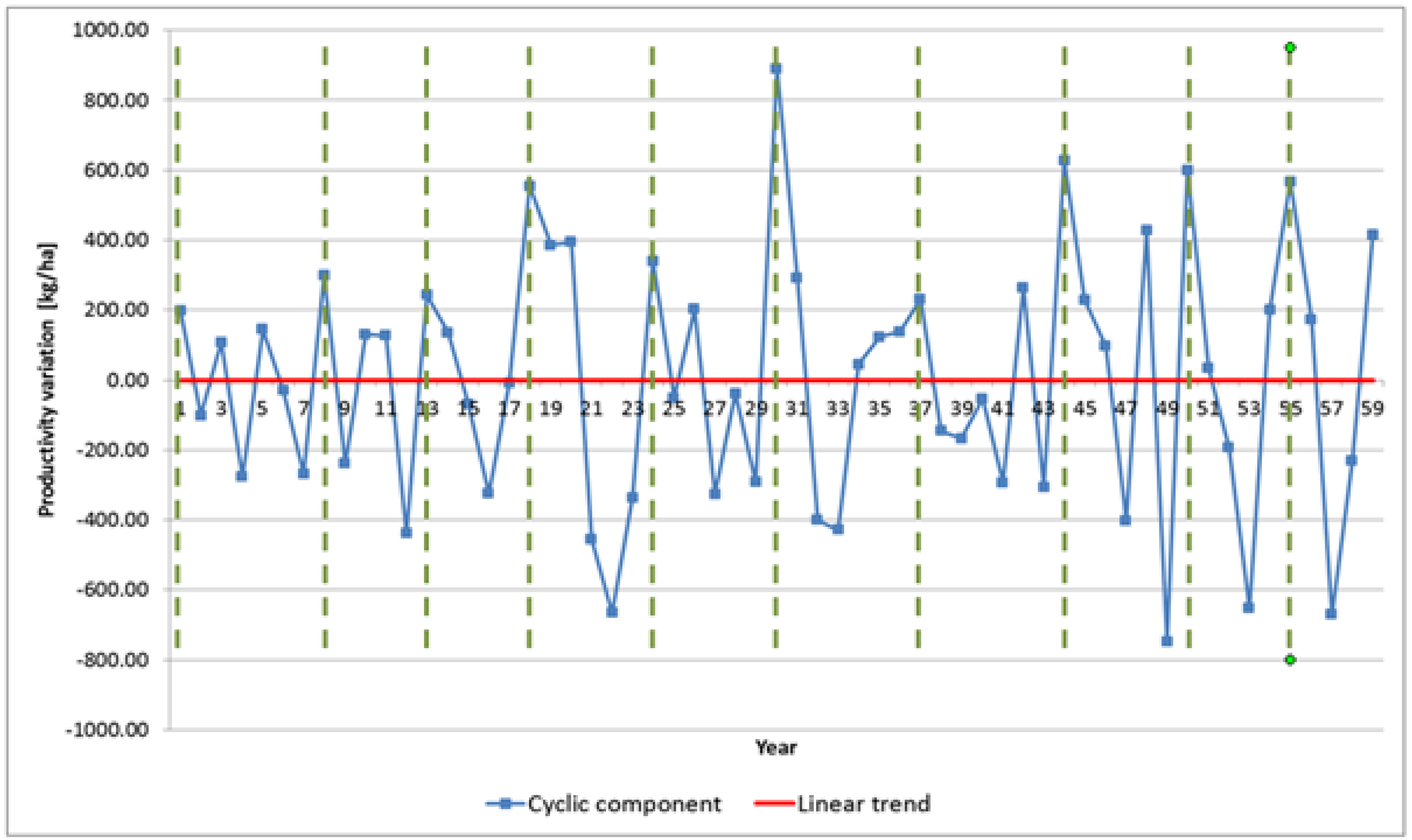
For example in Figure 4 the cyclical component for the grain yield in France, for a time period of 59 years, is represented. It should be noted that the trend of this component is almost horizontal, so it can be appreciated that the trend of the yield series used was well chosen. The data that corresponds to several countries were used as control data, because it covers a longer period of time (59 years) but it is only presented for the case of France, in order not to overload this work with similar graphics.

Step 2. Analysis of the Cyclical Component of Yield and Extraction of a Variation Pattern for each of the Analyzed Crops.

The cyclical component of a time series has been analyzed over time using different methods (e.g., Fourier series analysis). The evolution of crop yield does not have a clearly defined time constant variation, so mathematical techniques usable for regular cycles become inoperable. As it can be seen in Figure 4, the time variation of the cycles is between 5 and 8 years.

In order to identify the variation cycles of the yield of a crop in the analyzed period of time, the following heuristic criterion was defined: a cycle of variation is defined by two successive peaks (local maximums), where a peak is considered a local maximum if at least three successive values of the yield—which are located before and after this peak—are smaller than the peak value. In Figure 4 the peaks of the cyclic components for the yield variation of the cereal crop (grain) in France for a fifty nine-year period of time can be observed.

Taking into account that the planning is made for a future functioning period of time which could ensure the integral recovery of the investment a ten-year period was chosen, considering that the technological progress might lead to the necessity of replacing the equipment at the end of this time period.

In order to forecast the yield for a future ten-year period of time, a ten-year interval containing the most unfavorable cycle will be extracted out of the cyclic series. The selection of the most unfavorable cycle is realized by using the following heuristic criterion: it is considered that the most unfavorable cycle is the cycle which contains the greatest variation of the yield of the analyzed bio-energetic crop. This variation is defined by the absolute value of the difference between the highest and lowest values from that certain cycle.

This criterion was chosen because the high yield variations lead to variations of the final production of the liquid biofuels, which are reflected in important variations of the income that liquid biofuel producers have. The variations of the incomes induce variation of the cash-flow and represent a high risks for an investment, which have to be estimated and diminished.

In Figure 4, it can be observed that the cycle which has the highest yield variation is the cycle between the years 44–50, which present a variation of about 1400 kg/(ha·year) (yield variation from +620 kg/ha to −790 kg/ha).

For the analyzed time series the existence of cycles of 6–8 years can be observed. Because of this, to make an appraisal for a fixed ten-year period the selected cycle is completed with the number of consecutive values necessary to have ten values. The cycle selected for simulation will be completed with the values corresponding to years 51, 52 and 53 to get a complete series of ten years.

Step 3. Choice of the Cultivated Land Areas for Each of the Analyzed Crops in the Forecasted Period.

The land areas which will be cultivated with biofuel crop every year are chosen considering the need for crop rotation and economic interests of cultivators. For the case analysis of this paper we have chosen as variation model of the cultivated land areas their variation in the ten years preceding the forecast period. Obviously a more detailed analysis should include rules that determine the order of crop rotation (after a certain culture another one cannot be grown at random) and their frequency in a particular area, but the problem is beyond the aim of this paper.

Step 4. Determining of the Population Variation in the Forecasted Period.

Because the agricultural crops that were used for the liquid biofuels production are also being used for other purposes too (such as human alimentation, animal food, industry) when estimating the potential of each culture the coverage of these consumptions must be taken into account.

The data concerning the evolution of the population of a region for a future period of time can be imported from different sources (Eurostat, World Bank, etc.) or can be generated on the basis of particular scenarios, which are specific to that region.

For the case study that has been realized in this paper and for the analyzed countries, the forecast for the evolution of the population made by Eurostat has been accepted. The population variation for the analyzed countries (Romania, Italy and France) and forecasted for a ten-year period is presented below in

Table 1. The population variation in a forecast period (million residents). Source: [56].

Year	2016	2017	2018	2019	2020	2021	2022	2023	2024	2025
Romania	19,869	19,824	19,778	19,732	19,687	19,641	19,588	19,528	19,462	19,390
France	66,487	66,789	67,086	67,375	67,659	67,938	68,214	68,489	68,762	69,035
Italy	61,151	61,353	61,555	61,757	61,961	62,168	62,376	62,586	62,797	63,011

.

Step 5. Calculation of the Technical Potential for Each Type of Biofuel.

The technical potential is calculated for each crop as the difference between the production of the respective year i, and the consumption needs of the population and other sectors:

$${Potential}_i={Production}_i-Population\_need{s}_i$$

The production of the current year is determined as a product between yield and the analyzed crop acreage:

$${Production}_i=Yiel{d}_i\cdot Cultivated\_are{a}_i$$

The yield of a bio-energetic crop is estimated based on the variation cycle that was selected in the previous step and on the determined trend: yield_i = c_i + t_i.

The trend (t_i) can be considered constant or may vary in the forecast interval after a certain law variation (which is determined through known methods such as the least squares method). Considering the variation of the yield of a crop in time, which is presented in Figure 1, three different intervals can be observed:

(1)

The interval I—which has a slight increase of the agricultural yield—it does not present practical interest.

(2)

The interval II—which has a significant increase of the agricultural yield—it corresponds to the period of time when agricultural technologies that were being used developed.

(3)

The interval III—saturation interval—where the agricultural yield can only increase slightly due to the biologic limitations of the cultivated plants.

Choosing a constant or variable trend depends on the interval in which a region can be found from the agricultural yield point of view.

The needs for human consumption are determined on the basis of the average annual per capita consumption of each culture (e.g., cereals) or the intermediate product (sunflower oil) or the finished product (alcohol) and the volume of the population in the current year:

$$Population\_need{s}_i=Populatio{n}_i\cdot Consumption\_per\_capita$$

The potential that is estimated this way is based on the real variation of the yield which manifested in the past in a case that has been considered the most unfavorable for planning an investment. Obviously, when planning an investment, the most favorable case must be analyzed too, but the purpose of this research was to find a method for estimating the biofuel potential of a region. This estimation allows a most realistic appraisal of the investment risks (especially the income and cash-flow fluctuations), and their minimization by using adequate countermeasures.

Step 6. Establishing the Biofuel Needs for the Forecasting Period.

To establish the biofuel needs for a region a heuristic criterion has been taken into account, considering that if the transport is used to meet the needs of the population, it follows that the values of biofuel needs will depend on the size of population at the time of estimation. For this reason we have calculated an indicator of the average annual per capita consumption of fossil fuel.

It has been decided that this indicator will be calculated as an average of the specific consumptions for the past five years. This decision has been made because it has been considered that—on a regional scale—a five-year period of time correctly reflects the needs of the population from that region and the effect that the introduction of the technological progress would have in transport. Besides after analyzing the specific consumptions of different transportation vehicles which work with liquid fuels it has been concluded that they have comparable values for the same vehicle category regardless of the producer.

This fact shows that technology has reached a limit and a great improvement in the performance of vehicle engines is highly improbable.

$$Biofuels\_Nee{d}_i=Populatio{n}_i\cdot Specific\_consumption$$

Step 7. Comparative Analysis and the Necessary Technical Potential of Biofuels, Emphasizing the Surpluses and Deficits of Biofuel in the Analyzed Period.

Knowing the potential of a region for each type of biofuel, and also the quantity required for consumption, the level of demand coverage (%) for each type of biofuel can be calculated. Therefore the excess or shortage for each biofuel type, for every analyzed region, can be seen.

This analysis was considered to be useful especially for the government—when it came to the elaboration of strategies to implement biofuels sources—and also for producing companies in order for them to correctly dimensioning their investments. For these calculations were used the calorific value of 29.7 MJ/kg for alcohol and 37.2 MJ/kg for biodiesel.

4. Results and Discussion

In this section are presented the results of a case study that was obtained by applying the methodology shown in the previous section for three European Union member states: Romania, France and Italy.

The crops that have been analyzed for the biofuel production were the following: cereals, potatoes and sugar beet for bioethanol, and rapeseed, sun flower seed and soya, for biodiesel. In order to correctly estimate the potential of a region for a certain type of biofuel the following values for specific consumptions and transformation yields have been used.

For the ethanol production the following yields have been used:

• Cereals—38 liters absolute alcohol/100 kg
• Potatoes—12 liters of absolute alcohol/100 kg
• Sugar beet—9.5 liters of absolute alcohol/100 kg

For the production of biodiesel there has been used the following yields:

• 39% for the production of seed oil
• 75% for the production of oil biofuel

The specific consumption for human needs:

• Cereals (in wheat equivalent):

  (a)

  Romania: 214 kg/(capita·year)

  (b)

  Italy: 183 kg/(capita·year)

  (c)

  France: 302 kg/(capita·year)

• Alcohol: 9 l/(capita·year), for all three countries
• Sunflower oil:

  (a)

  Romania: 12 kg/(capita·year)

  (b)

  Italy: 15 kg/(capita·year)

  (c)

  France: 15 kg/(capita·year)

• Soya: none, but it will be considered that only the production that corresponds to 1/3 of the cultivated land area will be processed for biodiesel (in France and Italy), while the rest remains available for other necessities. In Romania, only for sugar beet crops and for soy—for objective reasons—was a constant surface considered, about a quarter of the agricultural area was considered unworked at the level of 2011, i.e., 228,250 ha.
• Rape: none, for all three countries.
• Sugar beet: for Romania a surface of 228,250 ha will be considered, whereas for Italy and France, the land areas that ensure a quantity of beet production calculated for covering the internal consumption that is at the level of 36.5 g/(day·capita) for France and 18.5 g/(day·capita) for Italy will be used.
• Potatoes: for Romania: 98 kg/(capita·year), and for France and Italy will be accepted the value: 88 kg/(capita·year).

4.1. Estimation of the Bioethanol Potential

In Romania the ethanol can be obtained in terms of economic efficiency from cereals, potatoes or sugar beet. For France and Italy this assumption was maintained even if in these countries it is possible to use these and other biological raw materials for biofuels production. Next, only these crops will be used to estimate the bioethanol potential for all three analyzed countries.

4.1.1. Estimation of the Bioethanol Potential from Cereals

As an example, in the following figure the results of the applied methodology for Romania will be presented. For France and for Italy only the final results will be presented for all bio-energetic crops.

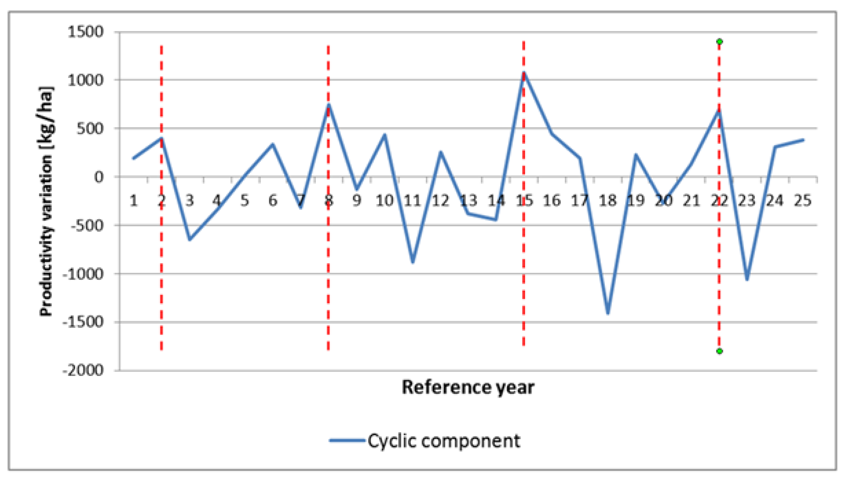
According to data gathered by the authors, the cereal crop yields in Romania, for a period of 25 years, between 1990 and 2014, vary as shown in Figure 5. We can observe the trend of this series and the cyclic component, extracted with the Hodrick-Prescott filter.

The variation of the cyclic component is described in Figure 6. It can be seen that for the periodicity a variation in cycles of about 6–7 years is observed, with limits of variation from −1400 to +1100 kg/ha, which is a pretty important variation of yield.

In order to estimate the bioethanol potential for the ten years period of time a variation cycle that is completed with 3–4 additional values from the series was adopted. For the example above a cycle of variation which comprises between years 15–22 is selected because it contains the maximum yield variation. That is completed with yield values corresponding to years 23 and 24.

The estimated cereal production for the considered period of time and for all three analyzed countries is shown in the table below (

Table 2. Estimated cereals production for the forecasted period (thousand tons). Source: authors’ own calculation based on National Statistics Institute database and [56].

Year	2016	2017	2018	2019	2020	2021	2022	2023	2024	2025
Romania	26,673	21,273	17,253	9155	17,892	15,596	17,112	20,958	12,155	20,439
France	71,868	70,015	69,594	64,868	71,681	59,301	72,429	67,198	65,608	62,819
Italy	18,898	18,483	17,745	18,534	16,978	17,540	20,764	16,955	17,186	18,703

).

Human consumption needs for cereals which are determined on the basis of the average annual consumption of 214 kg wheat equivalent per capita for Romania, 302 kg/capita/year for France and 183 kg/capita/year for Italy are presented below (

Table 3. Human consumption needs for cereals (thousand tones wheat equivalent). Source: authors’ own calculation based on [56].

Year	2016	2017	2018	2019	2020	2021	2022	2023	2024	2025
Romania	4261	4252	4242	4232	4223	4213	4203	4192	4179	4165
France	11,191	11,228	11,265	11,302	11,339	11,377	11,415	11,453	11,492	4261
Italy	4261	4282	4303	4325	4346	4368	4390	4412	4434	4456

).

The estimation of bioethanol production from cereals, corresponding to these three countries, after preserving the need for human consumption, is presented in

Table 4. Estimation of the bioethanol production from cereals (in million liters of absolute alcohol). Source: authors’ own calculation based on [56].

Year	2016	2017	2018	2019	2020	2021	2022	2023	2024	2025
Romania	7528	5481	3959	888	4214	3348	3930	5398	2061	5218
France	19,081	18,340	18,143	16,312	18,865	14,126	19,081	17,059	16,421	15,327
Italy	2378	2205	1909	2192	1585	1783	2991	1527	1599	2158

.

As it can be observed, there are significant variations between the values obtained every year for the three analyzed countries.

4.1.2. Estimation of the Bioethanol Potential from Potatoes

The estimated bioethanol production from potatoes is presented in the table below (

Table 5. The estimation of bioethanol potential from potatoes (million liters of absolute alcohol). Source: authors’ own calculation based on [56].

Year	2016	2017	2018	2019	2020	2021	2022	2023	2024	2025
Romania	302	242	266	230	219	258	168	269	66	161
France	188	77	75	122	259	74	104	102	139	193
Italy	0	0	0	0	0	0	0	0	0	0

).

4.1.3. Estimation of the Bioethanol Potential from Sugar Beet

The estimated production of bioethanol from sugar beet is shown in the table below (

Table 6. The estimated potential of bioethanol from sugar beet (million liters of absolute alcohol). Source: authors’ own calculation based on [56].

Year	2016	2017	2018	2019	2020	2021	2022	2023	2024	2025
Romania	940	837	805	711	864	915	871	790	573	765
France	2475	1967	2537	1985	2338	2435	2303	2404	2450	2768
Italy	0	0	0	0	0	0	0	0	0	0

). It was considered that the entire production of sugar beet obtained from the considered land area will be used for biofuels.

It can be observed that for Italy there is no bioethanol potential because the internal consumption for human needs exceeds the volume of internal sugar production.

4.1.4. Estimation of the Global Bioethanol Potential

The global bioethanol potential of a region is presented below which is obtained from all the analyzed bio-energetic crops (

Table 7. Estimation of global bioethanol potential (million liters of absolute alcohol). Source: authors’ own calculation based on [56].

Year	2016	2017	2018	2019	2020	2021	2022	2023	2024	2025
Romania	8770	6560	5030	1829	5297	4521	4969	6457	2700	6144
France	21,744	20,384	20,755	18,419	21,462	16,635	21,488	19,565	19,010	18,288
Italy	2378	2205	1909	2192	1585	1783	2991	1527	1599	2158

and

Table 8. Estimation of global bioethanol potential of a region (TJ). Source: authors’ own calculation based on [56].

Year	2016	2017	2018	2019	2020	2021	2022	2023	2024	2025
Romania	260.47	194.83	149.39	54.32	157.32	134.27	147.58	191.77	80.19	182.48
France	645.80	605.40	616.42	547.04	637.42	494.06	638.19	581.08	564.60	543.15
Italy	70.63	65.49	56.70	65.10	47.07	52.96	88.83	45.35	47.49	64.09

).

4.1.5. Establish the Coverage Level of Biofuels Demand for Romania

As an example (only for Romania) the last two steps of the methodology will be calculated. The gasoline demand for the estimated period is shown in the table below (

Table 9. Romania’s demanded fuel type gasoline (thousand TJ). Source: authors’ own calculation based on [56].

Year	2016	2017	2018	2019	2020	2021	2022	2023	2024	2025
Gasoline type demand	67	67	67	67	67	67	66	66	66	66

).

The coverage level of demand for gasoline by replacing it with bioethanol is shown in the table below (

Table 10. The coverage level of demand of gasoline by replacing them with bioethanol. Source: authors’ own calculation based on [56].

Year	2016	2017	2018	2019	2020	2021	2022	2023	2024	2025
Coverage level	306%	229%	176%	64%	186%	159%	176%	229%	96%	219%

).

It can be noticed that the coverage of the demand for gasoline with bioethanol varies greatly throughout the analyzed period of time showing that the variations of yields have significant effects.

4.2. Estimation of the Biodiesel Potential

In Romania the biodiesel can be—in terms of economic efficiency—obtained from rapeseed oil, sunflower oil or soybean oil. These crops will also be used for France and Italy.

4.2.1. Estimation of the Biodiesel Potential from Rapeseed

In

Table 11. The biodiesel potential for rapeseed (thousand tons). Source: authors’ own calculation based on [56].

Year	2016	2017	2018	2019	2020	2021	2022	2023	2024	2025
Romania	20.673	11.284	15.199	12.110	14.343	1.376	11.988	27.095	21.804	20.275
France	41.407	43.731	50.703	40.642	38.869	45.229	46.208	53.394	49.144	41.468
Italy	0.398	0.336	0.306	0.306	0.336	0.367	0.336	0.367	0.336	0.398

the biodiesel potential obtained from rapeseed is presented.

4.2.2. Estimation of the Biodiesel Potential Obtained from Sunflower

The biodiesel potential for sunflower is presented below (

Table 12. The biodiesel potential for sunflower (thousand tons). Source: authors’ own calculation based on [56].

Year	2016	2017	2018	2019	2020	2021	2022	2023	2024	2025
Romania	944	792	802	387	641	554	645	816	541	844
France	186.07	129.38	73.53	103.76	200.88	168.49	173.06	186.42	255.16	133.84
Italy	0	0	0	0	0	0	0	0	0	0

). For Italy the potential is null because the internal sunflower oil production do not cover the level of human consumption.

4.2.3. Estimation of the Biodiesel Potential from Soybean

The biodiesel potential obtained from soybean, for all three analyzed countries, is shown in the table below (

Table 13. Potential of biodiesel from soybean (thousand tons). Source: authors’ own calculation based on [56].

Year	2016	2017	2018	2019	2020	2021	2022	2023	2024	2025
Romania	352	313	262	156	258	242	318	264	169	281
France	16.43	12.00	8.98	5.94	11.96	15.00	8.66	10.28	11.51	21.63
Italy	66	57	58	59	63	63	61	49	58	67

).

4.2.4. Estimation of Global Biodiesel Potential

The total potential of biodiesel from the three crops, estimated for the three analyzed countries is presented below in the

Table 14. Global potential of biodiesel (thousand tons). Source: authors’ own calculation based on [56].

Year	2016	2017	2018	2019	2020	2021	2022	2023	2024	2025
Romania	1317	1116	1079	555	913	797	975	1107	732	1145
France	244	185	133	150	252	229	228	250	316	197
Italy	66	57	58	59	63	63	61	49	58	67

in the form of biodiesel quantity and in

Table 15. Global biodiesel potential (TJ). Source: authors’ own calculation based on [56].

Year	2016	2017	2018	2019	2020	2021	2022	2023	2024	2025
Romania	48,980	41,526	40,146	20,650	33,976	29,662	36,270	41,184	27,223	42,604
France	9073	6886	4956	5593	9364	8508	8479	9303	11,748	7326
Italy	2470	2133	2169	2206	2356	2357	2282	1836	2170	2507

in the form of his energetic equivalence.

The consumption of biodiesel estimated for Romania, is presented below along with biodiesel coverage (

Table 16. The consumer’s requirements for diesel fuel and the biodiesel coverage. Source: authors’ own calculation based on [56].

Year	2016	2017	2018	2019	2020	2021	2022	2023	2024	2025
The Consumer’s Requirements (PJ)
Romania	183.38	183.01	182.60	182.17	181.76	181.33	180.91	180.42	179.87	179.26
The Level of the Biodiesel Coverage (%)
Romania	26.7%	22.7%	22.0%	11.3%	18.7%	16.4%	20.0%	22.8%	15.1%	23.8%

).

As it can be noticed from the table above, the potential for Romania’s biodiesel only covers a small extent of the diesel demand in the analyzed period of time.

5. Conclusions

All investment projects are subjected to different risk category that may influence the implementation and the performances of the projects. The more realistic assessment of these risks allows the investors to take steps to reduce them.

The investment projects from the field of liquid biofuels production are also affected by risks, some of these risks being general and some of them being specific to the field. A special risk category for these types of investment projects is represented by the climatic factors.

In this work, a heuristic methodology that has been developed in order to forecast the potential for liquid biofuels in a certain area was presented, which is to be used as supplier of raw materials for the investment projects in liquid biofuels production.

Unlike other methodologies for estimating of the liquid biofuel potential, our methodology performs the estimation of the variation which may occur in the volume of biofuels production as an effect of the climatic factors during a time period which cover the duration of return for an investment project in this field. Because the number of factors that affect the quantities which are harvested from some crops is high and a lot of these factors cannot be quantified, only the cumulative effect on the yield of the analyzed crops was considered, which leads to annual variations for the value of this yield. The methodology will identify the most unfavorable case of the variation in the biofuel production through a heuristic approach to the problem.

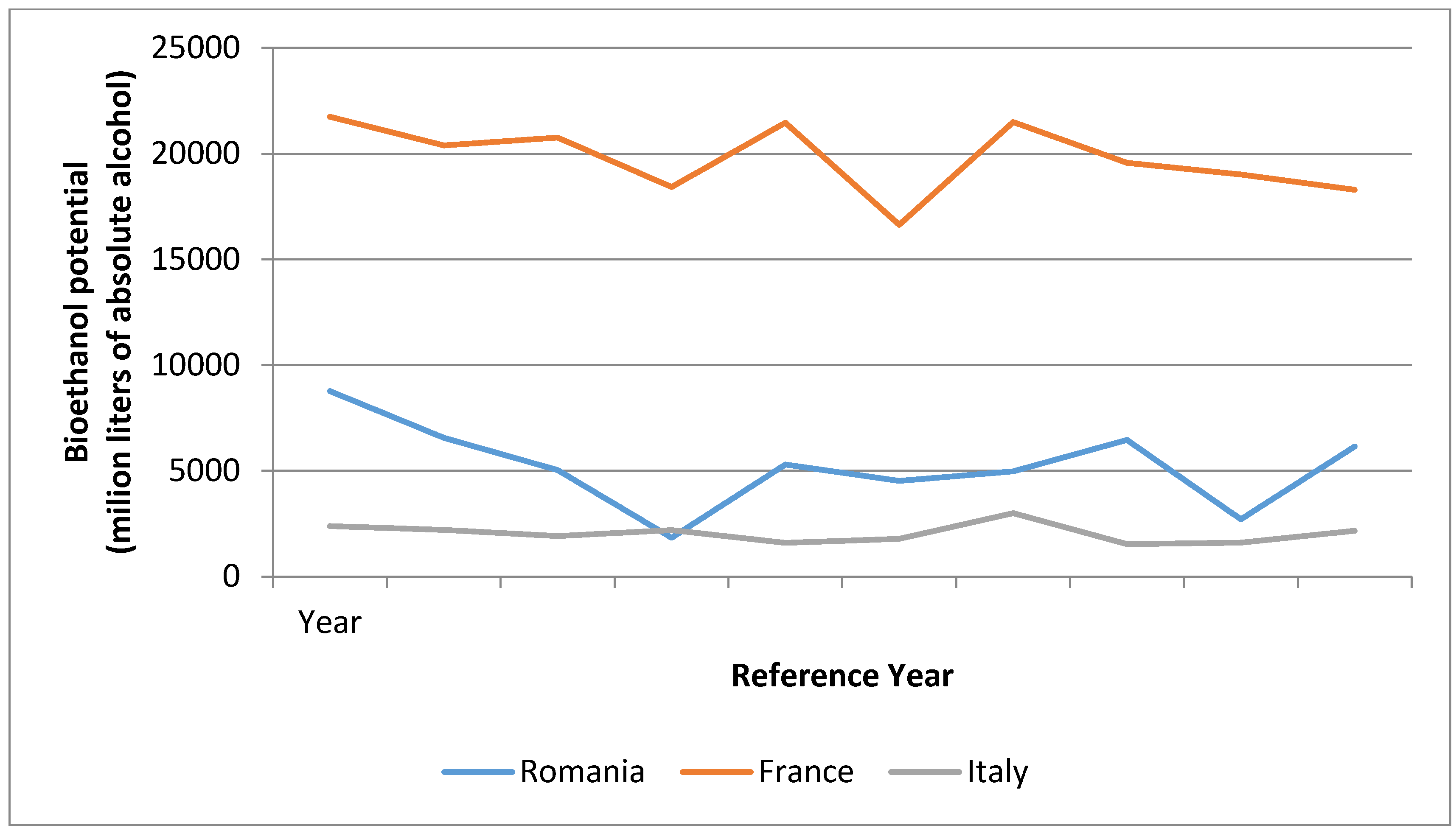
The results that were obtained by applying this methodology to three distinct regions that are represented by three countries from the EU—Romania, France and Italy—have confirmed the existence of some important variations in the liquid biofuels potential for the analyzed regions.

In Figure 7 it can be observed that the annual variations of bioethanol potential reach values of 3468 million liters of absolute alcohol for Romania, 4827 million liters of absolute alcohol for France and 1464 million liters of absolute alcohol for Italy.

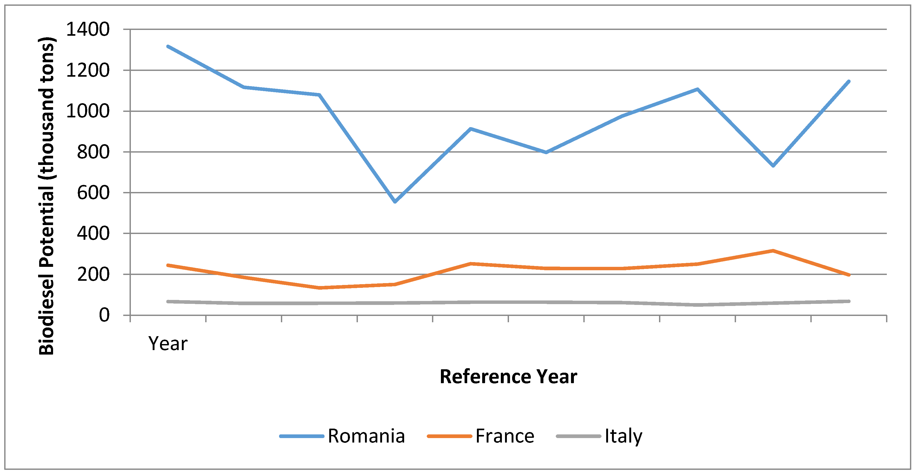
For the biodiesel potential the annual variations (Figure 8) reach values of 524,000 tons for Romania, 119,000 tons for France and 12,000 tons for Italy.

Also taking into account that presented and designed methodology is a heuristic one, the future evolution of biofuel potential according to determined values cannot be guaranteed. Since the used data describe the cyclic behavior of crops yield—behavior determined by the cyclic variation of climatic factors—will be obtained a realistic image of the evolution of biofuels potential of a region for a future time horizon.

Risk reduction measures which are induced by the liquid biofuels potential variations on the economic efficiency of investment projects from this field remain valid and usable, even if in the forecasted period yield variations do not respect the estimated model constructed with the aid of the presented methodology.

Obviously the methodology presented above is just a beginning. More accurate results can be obtained by refining the input data and their analysis by small region because the yield of a crop is not constant throughout a region. For the future the implementation of the methodology into a software application that will permit the analysis of a large number of possible scenarios for a specific region is envisaged.