A Power Balance Aware Wireless Charger Deployment Method for Complete Coverage in Wireless Rechargeable Sensor Networks

Abstract

Traditional sensor nodes are usually battery powered, and the limited battery power constrains the overall lifespan of the sensors. Recently, wireless power transmission technology has been applied in wireless sensor networks (WSNs) to transmit wireless power from the chargers to the sensor nodes and solve the limited battery power problem. The combination of wireless sensors and wireless chargers forms a new type of network called wireless rechargeable sensor networks (WRSNs). In this research, we focus on how to effectively deploy chargers to maximize the lifespan of a network. In WSNs, the sensor nodes near the sink consume more power than nodes far away from the sink because of frequent data forwarding. This important power unbalanced factor has not been considered, however, in previous charger deployment research. In this research, a power balance aware deployment (PBAD) method is proposed to address the power unbalance in WRSNs and to design the charger deployment with maximum charging efficiency. The proposed deployment method is effectively aware of the existence of the sink node that would cause unbalanced power consumption in WRSNs. The simulation results show that the proposed PBAD algorithm performs better than other deployment methods, and fewer chargers are deployed as a result.

1. Introduction

In the past, due to the limitations of battery power, the lifetimes of sensors used in wireless sensor networks heavily depended on the energy provided by the batteries, which made the stability of the whole network greatly uncertain. Various scholars have put forward a range of studies in attempts to solve the problem of limited battery power, including the use of effective routing protocols [1], efforts to ensure efficient energy consumption [2], and so on. However, the above research did not succeed in solving the problem in a fundamental way. Although the advances they proposed can effectively extend the lifespan of the network, the network will still become unusable in the end when the sensors run out of battery power. In addition, if the sensors in a network rely on solar power provided by the sun, the sensors and the overall efficiency of the network will be affected by various environmental factors. In fact, a number of factors can make a sensor unable to operate effectively for extended periods of time. In order to overcome the power constraints of sensing devices, various discussions relating to the concept of wireless power transmission have been started in recent years [3], and the related studies have provided some solutions to the limited lifetimes of wireless sensor networks. Through chargers, electric power is transmitted to radio-frequency identification (RFID) tags [4], sensing devices [5], and terminal equipment. Due to the convenience and rapid development of wireless charging technology, it has attracted the attentions of both academic scholars and industrial professionals. According to the TechNavio market research analysis and forecast [6], the annual growth rate of the global wireless charging market will be more than 33% in 2020—this shows that this field has great potential.

How to improve the survival time of wireless sensor networks using wireless power transmission technology is thus a topic that is currently widely discussed and studied [6,7]. These new types of networks, which enable the use of wireless charging to prolong the lifespan of the network sensors, are called wireless rechargeable sensor networks (WRSNs). In order to make the sensors within the sensing region maintain stable power, the deployment of the wireless chargers becomes the primary consideration. Due to cost considerations, the number of chargers in the region should be minimized to the greatest extent possible. On the other hand, the amount of power supplied to a sensor has an important influence on the performance of the sensor. Therefore, effectively minimizing the number of wireless chargers used in the deployment while also maximizing the charging ability of the wireless chargers is the goal of this research.

Although many studies relating to the deployment of wireless chargers have been published in recent years, these studies did not take into account some important factors. For example, previous research has solved the sensor coverage problem without calculating charging power and without considering the existence of the sink node. To overcome these limitations, this study aims to investigate how to set up X directional chargers in a given area. Previous studies assume a uniform power consumption of the sensor nodes, but this is not the case in a realistic setting. The data sink node collects sensing data from all the sensor nodes, and sensor nodes nearby the sink need to facilitate more data forwarding than sensor nodes far away from the sink, so the power consumption of the nodes close to the sink is larger and the area near the sink is called the hot zone [8]. The sensor nodes in the hot zone run out of battery power more quickly than sensor nodes outside the hot zone. When the sensor nodes in the hot zone run out of battery power, the sensor network fails to work properly and this phenomenon is the famous “energy hole problem” [9]. No matter in wireless sensor networks (WSNs) or WRSNs, multi-hop transmission is employed to forward data back to the sink node and the appearance of the energy hole will interrupt the communications. Figure 1 shows the concept of the multi-hop transmission and demonstrates how the sensor nodes in the hot zone take the responsibility of forwarding the data to the sink node.

Wireless charger deployment problems have attracted substantial attention in recent years. We review a number of the relevant previous studies. He et al. [10] focused on the omnidirectional wireless charger deployment problem and deployed charging devices in the sensing area of interest to provide enough charging power to maintain the operation of the network, but they explored the space with a more traditional triangle solution. Chiu et al. [11] divided the sensing areas into grids and placed omnidirectional wireless chargers on various grid points. Their deployment also took into consideration the moving paths of mobile sensors. In a study by Liao [12], the coverage area of the chargers was conical, and the sleep schedule of the chargers was considered in order to reduce the power consumption. Compared with the aforementioned studies of omnidirectional wireless chargers, studies by Horster and Lienhart [13,14] considered the deployment of the directional chargers and defined the charging area of a directional charger as a sector with a given angle. In the Horster and Lienhart study [13], triangles were used to represent the charging area of directional chargers, so an integer linear programming solution was proposed in which each grid point represents a possible location of the deployment. The Han et al. study [14], meanwhile, minimized the number of deployed chargers while also considering the connections among chargers. The reviewed literature is organized in

Table 1. Literature comparisons.

Name	Type	Contribution	Power Balance Aware
Energy provisioning in wireless rechargeable sensor networks. [10]	Omnidirectional charger	Physical characteristics of wireless charging	No
Mobility-aware charger deployment for wireless rechargeable sensor networks. [11]	Omnidirectional charger	A sensing model for optimization of mobile deployment	No
Optimized charger deployment for wireless rechargeable sensor networks. [12]	Omnidirectional charger	Charger sleep scheduling	No
Minimizing charging delay in wireless rechargeable sensor networks. [15]	Omnidirectional charger	Robot stop locations in discrete areas	No
Approximating optimal visual sensor placement. [13]	Directional charger	Grid linear programming	No
Deploying directional sensor networks with guaranteed connectivity and coverage. [14]	Directional charger	Considers the fact that the sensors are connected to each other	No

below. Interestingly, these studies did not consider the unbalanced power consumption effect caused by forwarding data to the sink node. Such unbalanced power consumption can make the sensor nodes near the sink rapidly lose power.

2. Experimental Section

2.1. Problem Statement

First, we define the basic assumptions of the WRSN model. This is then followed by an introduction of the charger coverage Equation and the charging power Equation. The definition of charging demand and the effects of the data sink node are also given.

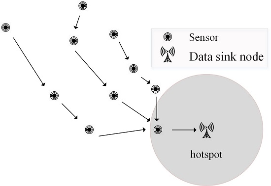
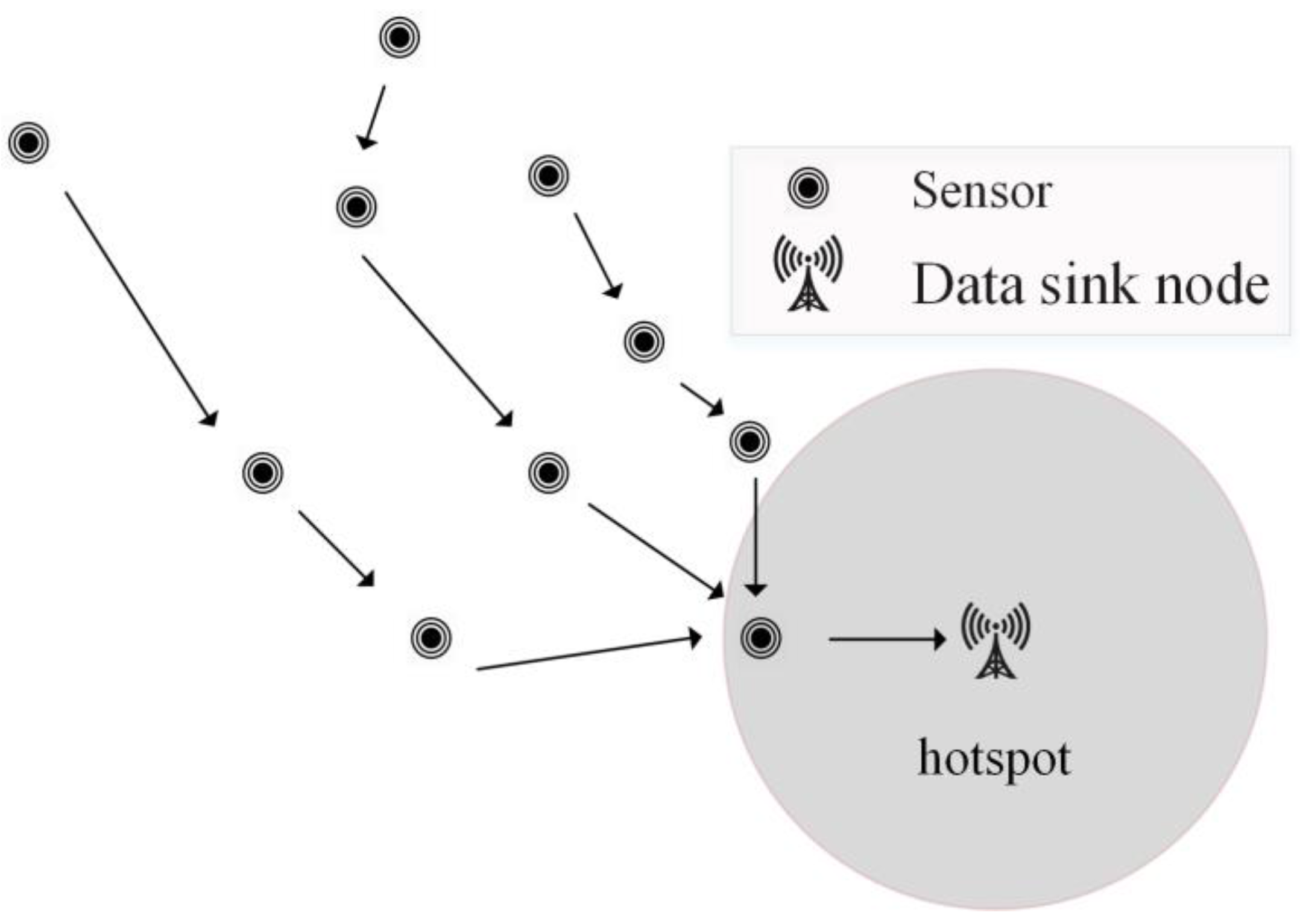
2.1.1. The WRSN Model

Given a two-dimensional region Z, assume that this space has X rechargeable sensors and make them a collection of S = {s₁,s₂,…,s_X}. The data sink node, which is labeled as Y, exists in Z. The locations of the sensors and data sink node are known. The objective is to deploy M directional chargers. Define M directional chargers as A = {a₁,a₂,…,a_M}. Each charger can be deployed anywhere in the region, and a given directional charger can be placed at any angle. Assume that the chargers must cover a subset of the sensors S, regardless of the fact that all the chargers have the same charging efficiency. Past studies have failed to consider the existence of the data sink node and this defect can have significant impacts on the wireless charger deployment. In Section 2.1.3, we will explain the difference between charging efficiency and charging demand. According to the study by Garey and Johnson [16], the deployment of the chargers is a nonlinear programming problem, so it belongs to the category of non-deterministic polynomial-time hard (NP hard) problems and thus it is challenging to solve the charger deployment problem.

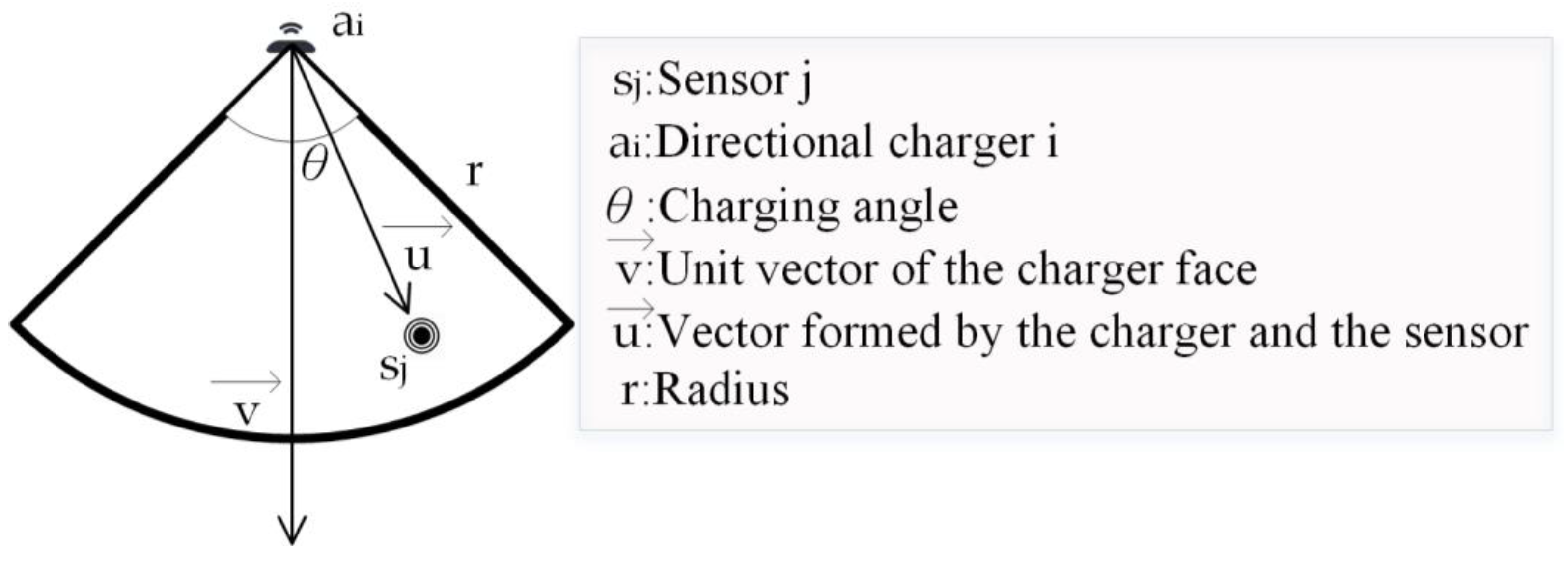
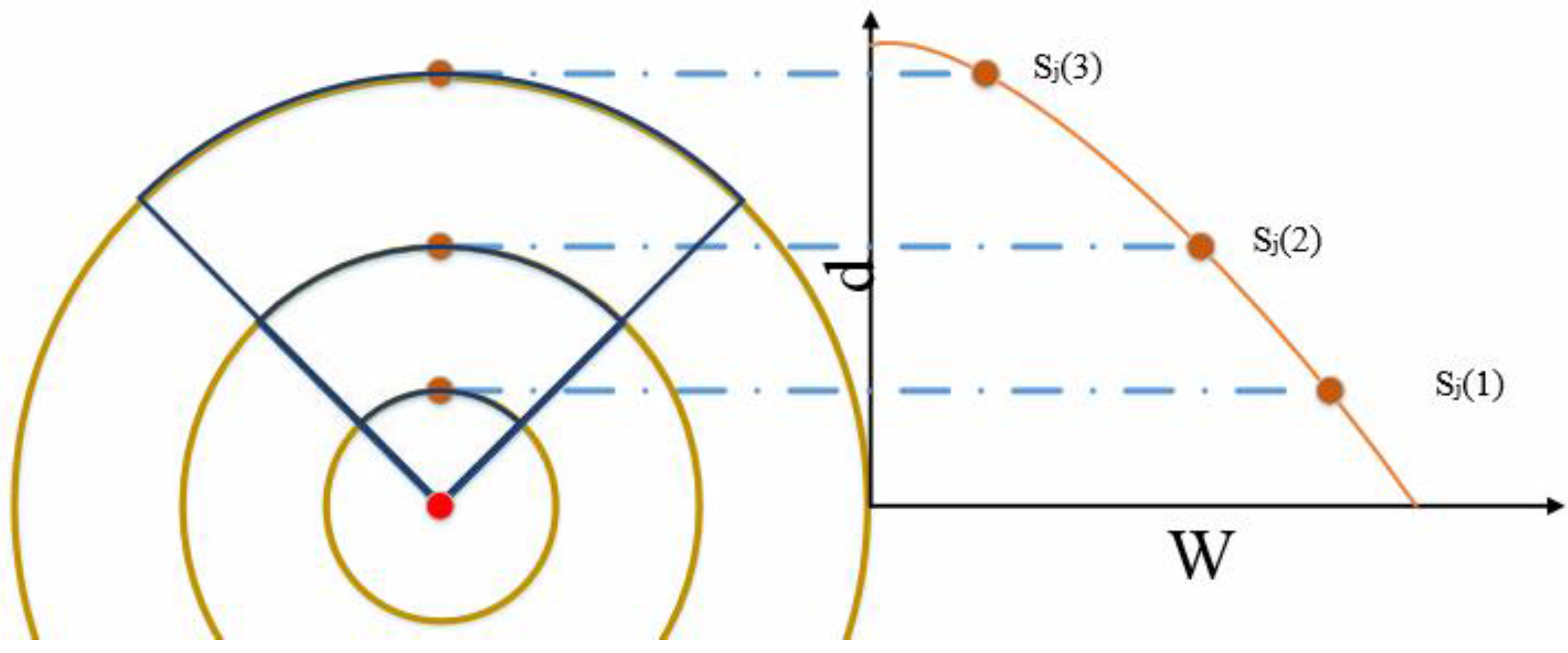
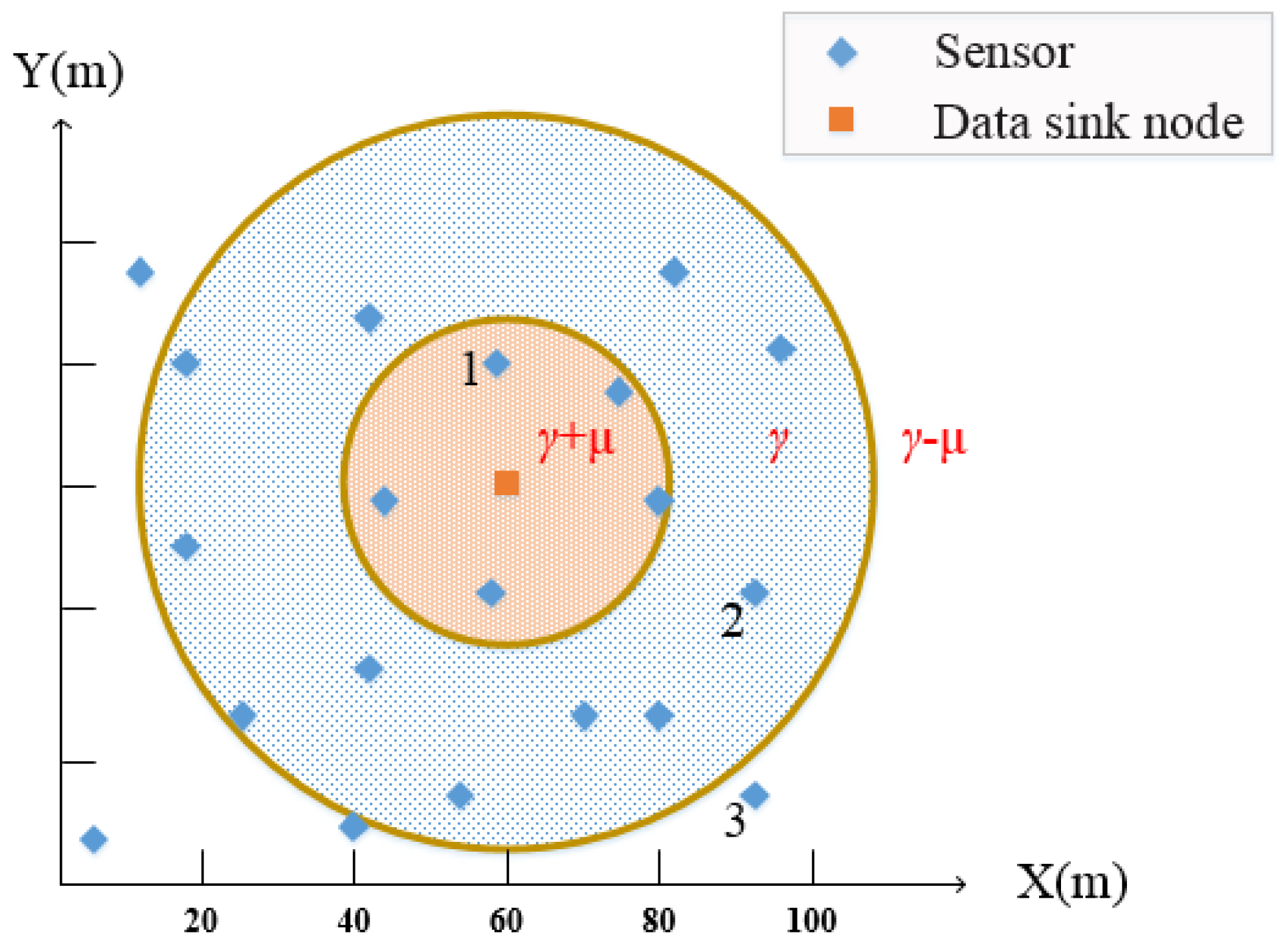
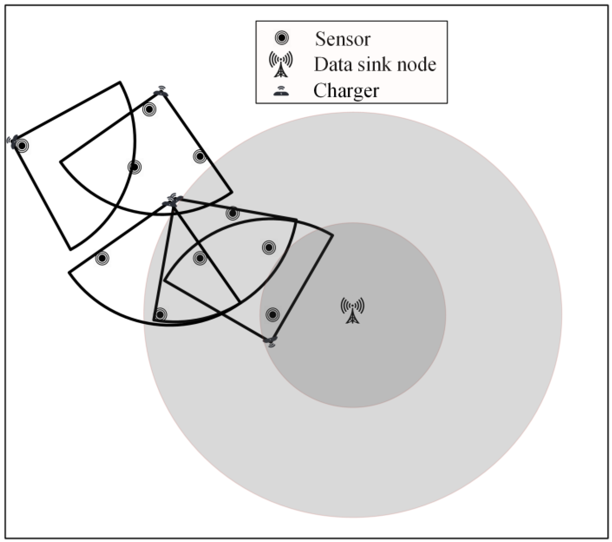
2.1.2. Coverage Area and Charging Power Model

In this section, we will illustrate the different types of chargers and why we have selected the directional chargers for deployment.

A. Omnidirectional Chargers

According to previous studies by He et al. and Chiu et al. [7,8], in the past, the coverage area of the omnidirectional charging model assumed the same charging ability and the equal charging distances. In fact, however, the received power attenuates when the distance increases and eventually the received power will be decreased to zero when a critical distance is reached. The charging coverage area of an omnidirectional charger is assumed to be a disk and the charger is assumed to be at the center of the charging area.

B. Directional Chargers

According to previous studies by Liao [12,13], the coverage area of the charging model is a sector, and products from different companies have charging angles with different ranges. Due to their relatively stable power coverage and low cost, directional chargers are often used in wireless rechargeable sensor networks.

Figure 2 is a schematic diagram of the coverage area of a directional charger. As shown in Figure 2, the directional charger a_i with angle θ charges the sensor s_j, and the radius is r. The arrow is directed out from the face of the charger. $\overrightarrow{\mathrm{v}}$ is a unit vector of the charger face, and $\stackrel{\rightharpoonup }{u}$ is the vector formed by the charger and the sensor. According to Ai and Abouzeid [13], the following Equation can be used to determine whether the sensor s_j is in the coverage area.

$$D(a_i,\stackrel{\rightharpoonup }{v},s_j)=\{\begin{array}{cc}1,& if\stackrel{\rightharpoonup }{v}\cdot \stackrel{\rightharpoonup }{u}-||\stackrel{\rightharpoonup }{u}|{|}_2\cos (\frac{\theta }{2})\ge 0\\ 0,& if\stackrel{\rightharpoonup }{v}\cdot \stackrel{\rightharpoonup }{u}-||\stackrel{\rightharpoonup }{u}|{|}_2\cos (\frac{\theta }{2})<0\end{array}$$

(1)

Equation (1) determines whether the sensors are in the coverage area, and when the value is 1, the charger’s charging power is calculated according to Equation (2).

$$E(dist(a_i,s_j))=\{\begin{array}{cc}\frac{\alpha }{(dist(a_i,s_i)+\beta ))},& dist(a_i,s_i)\le r\\ 0,& dist(a_i,s_i)>r\end{array}$$

(2)

In Equation (2), we define dist(a_i,s_j) as the Euclidean distance between the location of charger a_i and the location of sensor s_j, and $\alpha =\frac{\xi W_0{G}_a{G}_s}{C_W}{(\frac{\lambda }{4\pi })}^2$ where λ is the wavelength, and ζ is the efficiency of the rectifier. G_a and G_s are the antenna gain of the charger and the sensor, respectively. W₀ is the charging power, C_w is the antenna polarization loss, and β is the compensation parameter for short range transmission [17]. When the distance is larger than the charging radius r, the charging power is 0. According to Dai et al. [18], although the total power may not be precise, the total power can still be expressed as a function of the following Equation (3).

$$W(j)={\displaystyle {\sum }_{i\in M}D(a_i,\stackrel{\rightharpoonup }{v},s_j)}E(dist(a_i,s_j))$$

(3)

2.1.3. Charging Efficiency and Charging Demand

The data sink node is an important piece of equipment in wireless sensor networks. Sensors within the sensing area can collect data and send data back to the data sink node by multi-hops. If a sensor is close to the data sink node, then it will facilitate other sensors to forward data to the sink frequently, thus incurring more power consumption. The charging efficiency defines the charging ability of a charger, and different manufacturers have different charging efficiencies. The charging efficiency can be defined as the following Equation (4):

$$P(W(j))=\{\begin{array}{cc}\sigma \cdot W(j),& W(j)\le W_{\max }\\ \sigma \cdot W_{\max },& W(j)>W_{\max }\end{array}$$

(4)

The σ is a rechargeable factor and W_max is the charging efficiency limit of the sensor. In fact, for different brands of sensors, the values of σ and W_max are different. Here, however, we assume that all sensors have the same σ and W_max in the sensing region. From Equation (4), we can know that the charger does not have unlimited charging efficiency, so there is no instant charging in this setting. The sensors must have enough charge to maintain their normal operations, and if there is excess charge power, the excess power will be wasted. In a real environment, the charging demand of a sensor is related to the distance between the sensor and the data sink node, so we define charging demand as Equation (5). If the distance to the sink node is f, the charging demand is γ and μ is added/subtracted when the distance is greater/smaller than f.

$$H(dist(a_i,Y))=\{\begin{array}{cc}\gamma +\mu ,& dist(a_i,Y)<f\\ \gamma ,& dist(a_i,Y)=f\\ \gamma -\mu ,& dist(a_i,Y)>f\end{array}$$

(5)

Due to the charging power being a continuous value, deployed positions will have infinite points. Without discretization, a large amount of computation time is unavoidable. In order to design an efficient algorithm, we will further elaborate the discretization in the fourth chapter.

Table 2. Symbols used in this research.

Symbol	Corresponding Meaning
Z	Selected 2D region
x	Number of sensors
sj	The sensor j
m	The number of chargers
ai	The charger i
Y	The data sink node
θ	Charging angle
r	Charger radius
$\overrightarrow{\mathrm{v}}$	Direction vector of a charger
$\stackrel{\rightharpoonup }{u}$	The vector of the charger and sensor
σ	The factor affecting charging effect
Wmax	Upper bound value of charging power
γ	The average charging demand
μ	The charging demand adjustment coefficient
f	The specific distance which influences the charging demand

briefly explains all the symbols used in this study.

2.2. Method

This paper deploys directional chargers to cover the sensors in the sensing region. Moreover, a greedy algorithm is adopted to calculate the coverage and consideration of the influence of the data sink node is the premise utilized to obtain full coverage and to maximize the charging power. The proposed method called power balance aware deployment (PBAD) can be divided into two steps. First, the selected area is divided into a number of sub-regions, so that each sub-region can have a constant degree of charging power and charging demand. Then each sub-region is further analyzed to discover the minimum dominating sets (MDSs), and then the charging power is taken into consideration to select the optimal dominating set.

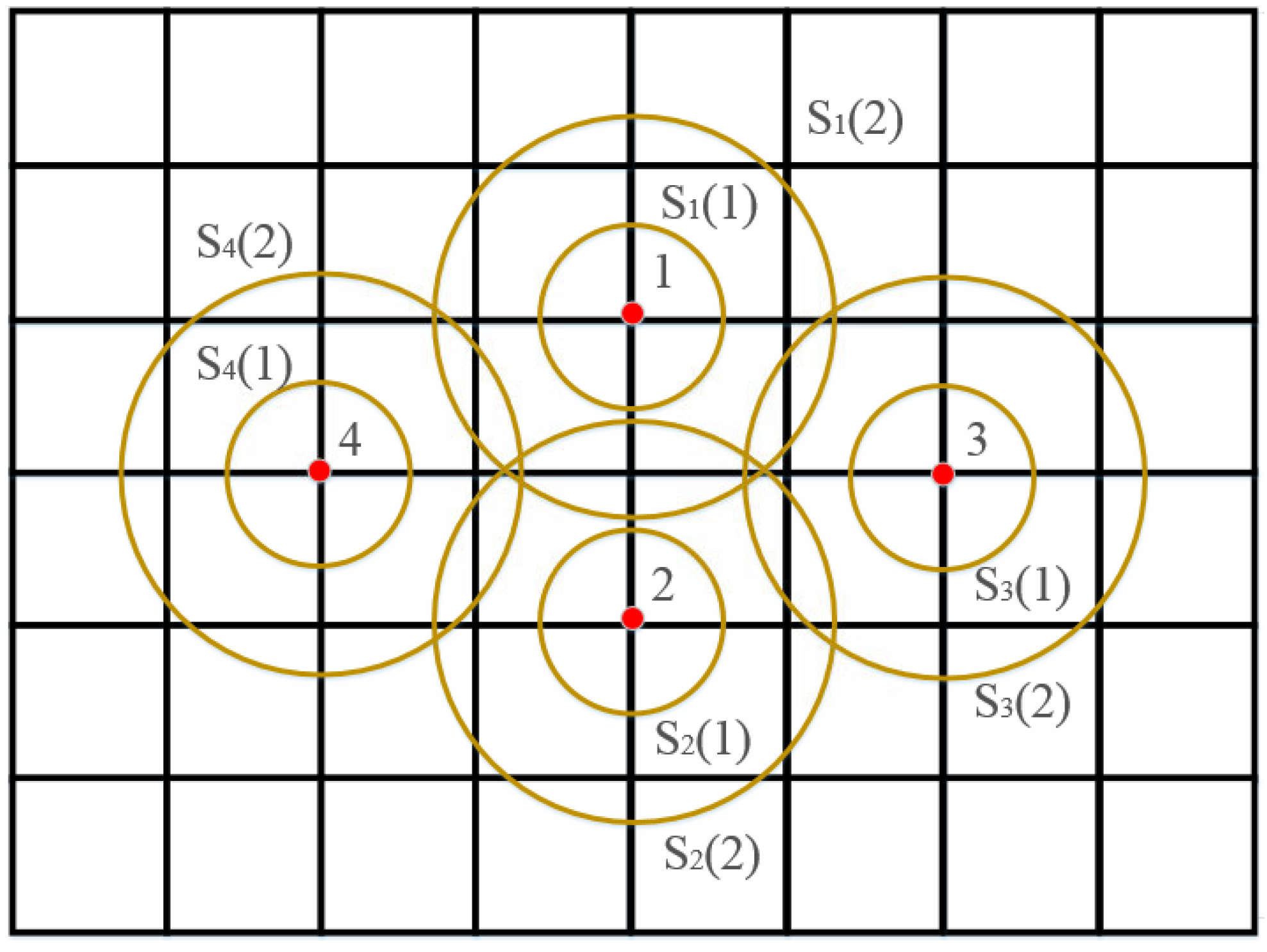
2.2.1. Area Discretization of Charging Power and Charging Demand

In a real environment, the chargers can be deployed in an infinite number of positions and give the sensors different charging effects. In order to be able to effectively deal with the problem, Fu et al. [15] suggested that the selected area should be discretized into finite sub-regions, so that the number of candidate points can be limited to a finite number of points. Due to different charging powers for sensors in different ranges, as shown in Figure 3, the charger can generate a certain charging power to sensors in each area. The charging power in the interval [S(X−1),(X)] is approximated to W(S(X)).

Figure 4 shows that the whole area is divided by eight homocentric circles into 15 sub-regions (including the area where the power is 0). The sensors placed in the same area will receive the same charging power.

As illustrated in Section 3, due to the existence of a data sink node in the real environment, each sensing power charging demand will vary. Because of the multi-hop characteristics in data transmission, sensors close to the data sink node will be used more frequently. In order to be able to find the minimum dominating set needed to meet this requirement, the sensing area must first be discretized, and the sensors are clustered according to the distances to the data sink node, as shown in Figure 5 below. The blue points represent the sensors. Two parameters, γ and μ, are used to cluster the sensors into three groups. The parameter γ is the threshold of the average charging demand and the parameter μ is the adjustment coefficient. According to different charging demands, the charger deployment locations are calculated.

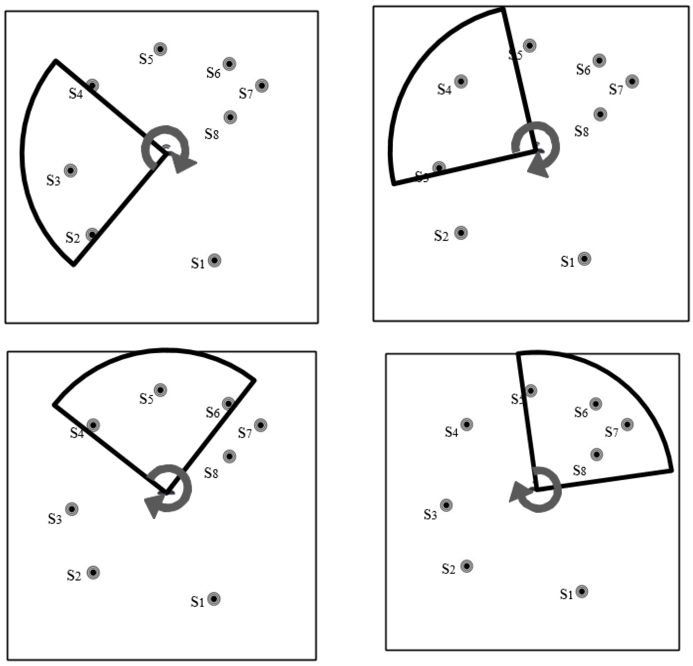
2.2.2. Searching for Minimal Dominating Set

In the previous section, the discretization of the region is elaborated and the next step is to discover the minimal dominating set from all the dominating sets. Therefore, this section mainly discusses the minimal dominating set. Two definitions are given first.

Definition 1. 

Given two sets of sensors under coverage, S_i and S_j, if S_i ⊆ S_j, then S_j dominates S_i.

Definition 2. 

If there is no other set dominating S_j in the region, then S_j will be determined to be the optimal dominating set in the region.

In order to find the optimal dominating set, we first assume that a charger is placed on a fixed point in the region. It is then rotated through different directions in order to determine all the coverage dominating sets, after which the best dominating set is selected. The minimal dominating set in the region is the optimal dominating set of the directional chargers. There is no need to calculate all of the coverage sets, because the target area has already been separated, so the charging powers in the same area are the same.

Algorithm 1: Calculate the Coverage Dominating Sets of Given Sensors

Input: Directional charger ai, angle θ and the sensor set Si with the locations of all the sensors

Output: Coverage Dominating Sets CDSs

Step 1. Calculate the included angle between the sensor and the charger;

Step 2. Sort sensors using angles, from small to large. θ1 ≤ θ2 ≤…≤ θX with respect to sensors s1, s2,…sX;

Step 3. Set a parameter St to record the current coverage set. Two parameters, θmin and θmax, record the minimum and maximum of the current coverage set. Initialize θmin = θ1, θmax = θ1; St = {s1};

Step 4. Starting from second sensors, j = 2;

Step 5. Rotate the chargers until no more sensors can be covered.

While (θj − θmin ≤ θ){

θmax = θj;

Add sj to St;

j = (j + 1) mod X;

}

Step 6. Add the current St to the cover dominating sets CDSs;

Step 7. Let θmax = θj and add sj to St;

Step 8. Remove the sensor from the smallest angle until the current set can be covered again

While(θmax − θmin > θ){

From the St to remove the minimum angle sensor, and θmin update into the current minimum angle value;

If(θmin=θ1){

End;}

}

Go to Step 5.

The above Algorithm 1 can be regarded as one kind of greedy algorithm. The coverage dominating sets are obtained through continuous rotations of the directional chargers, and then the optimal dominating set is selected from the calculated coverage dominating sets, as such, the region can be covered with the least amount of chargers. Steps 1 to 3 initialize the angles and Steps 4 to 7 rotate the angles and discover the angle that can cover the maximum number of sensors and label the sensors as a coverage dominating set. Step 8 removes the sensor with the smallest angle until the current set can be covered again. Figure 6 shows an example of finding the coverage dominating sets through rotations. The algorithm starts from the first coverage dominating set {s₂, s₃} and then discovers three more dominating sets, {s₃, s₄}, {s₄, s₅, s₆}, and {s₅, s₆, s₇, s₈}.

After discovering all the coverage dominating sets CDSs, the total power P, charging efficiency W and charging demand H are then calculated. The coverage dominating set with minimum H-W is selected as the best dominating set. The following algorithm II illustrates the procedures of finding the best dominating set. Figure 7 shows a best dominating set example obtained using the power balance aware deployment (PBAD) algorithm.

Algorithm 2: Search for the Best Dominating Set

Input: Coverage Dominating Sets CDSs

Output: The Best Dominating Set BDS

Step 1: Calculate the total power P and the charging efficiency W of all Coverage Dominating Sets CDSs using Equations (3) and (4)

Step 2: Calculate the charging demand H of all Coverage Dominating Sets CDSs using Equation (5)

Step 3: Select the best dominating set BDS with minimum H-W

3. Results

In this section, the simulations are conducted to verify the performance of the proposed approach. We compare the proposed power balance aware deployment (PBAD) algorithm with the location merging design (LMD) proposed by Fu et al. [15] and random deployment.

3.1. Description of Parameter Setting and Comparisons

We use the following parameters to set up the experiment: sensors are placed in a two-dimensional space measuring 100 m × 100 m. The number of sensors is 20 (X = 20), and the charging power model parameters of the chargers are α₁ = 80, β₁ = 40, d₁ = 16, and θ₁ = 90. The upper bound value of the average charge demand f_up = 30 m and f_low = 10 m. W_max = 40 mW, σ = 1, μ = 4 mW, and γ = 28 mW.

The proposed PBAD method is compared with the random position and random orientation (RPRO) approach and the aforementioned LMD. The following data are the values resulting from the respective implementations of our method, the RPRO, and the LMD for 300 simulations. Because LMD uses omnidirectional chargers for the deployment, it also uses different parameters. Specifically, those parameters are α₂ = 70, β₂ = 50, d₂ = 10, and θ₂ = 360.

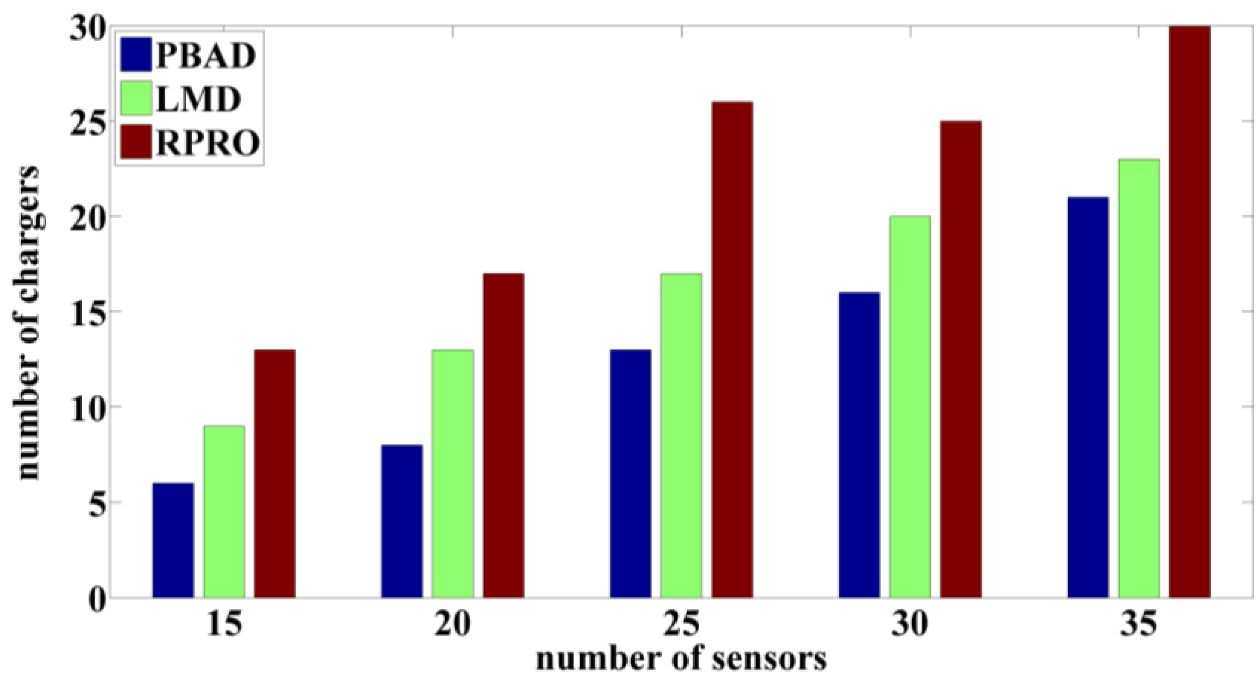
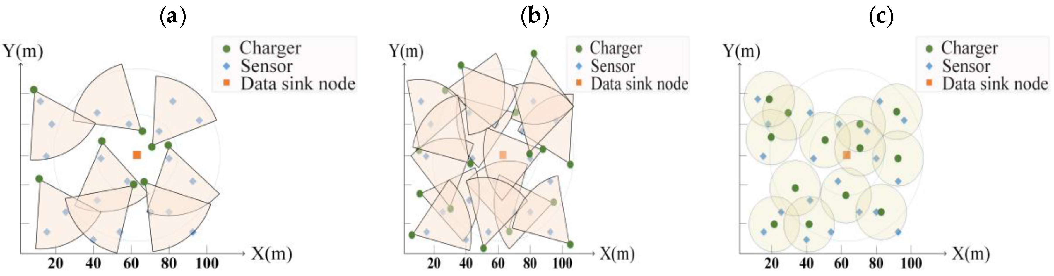
3.2. Experimental Results

We demonstrate the results using different numbers of chargers, different numbers of sensors, and different charging demands to show that the proposed PBAD algorithm achieves better coverage and has better charging power. The performance of the charging efficiency of each sensor is also given.

Satisfying all the charging demand for the deployment of the chargers is our main purpose. As can be seen from Figure 8 above, our method uses eight chargers to achieve this purpose. Compared with the RPRO and LMD approaches, the deployment generated by our approach is better. While the LMD approach only takes the power of charging into consideration, it does not consider the existence of the data sink node. Also, the charging power of an omnidirectional charger is poor, so the effect is poor. Without a doubt, the RPRO is the worst among the three algorithms.

4. Discussion

4.1. Effects of the Sensor Quantify on Charger Quantity

As can be seen from Figure 9, regardless of the number of sensors, the proposed PBAD method outperforms the other two algorithms and utilizes fewer amounts of chargers. It can be found that there is a slightly drop of the RPRO method at the number of 30 sensors, and this is due to the random nature of RPRO approach.

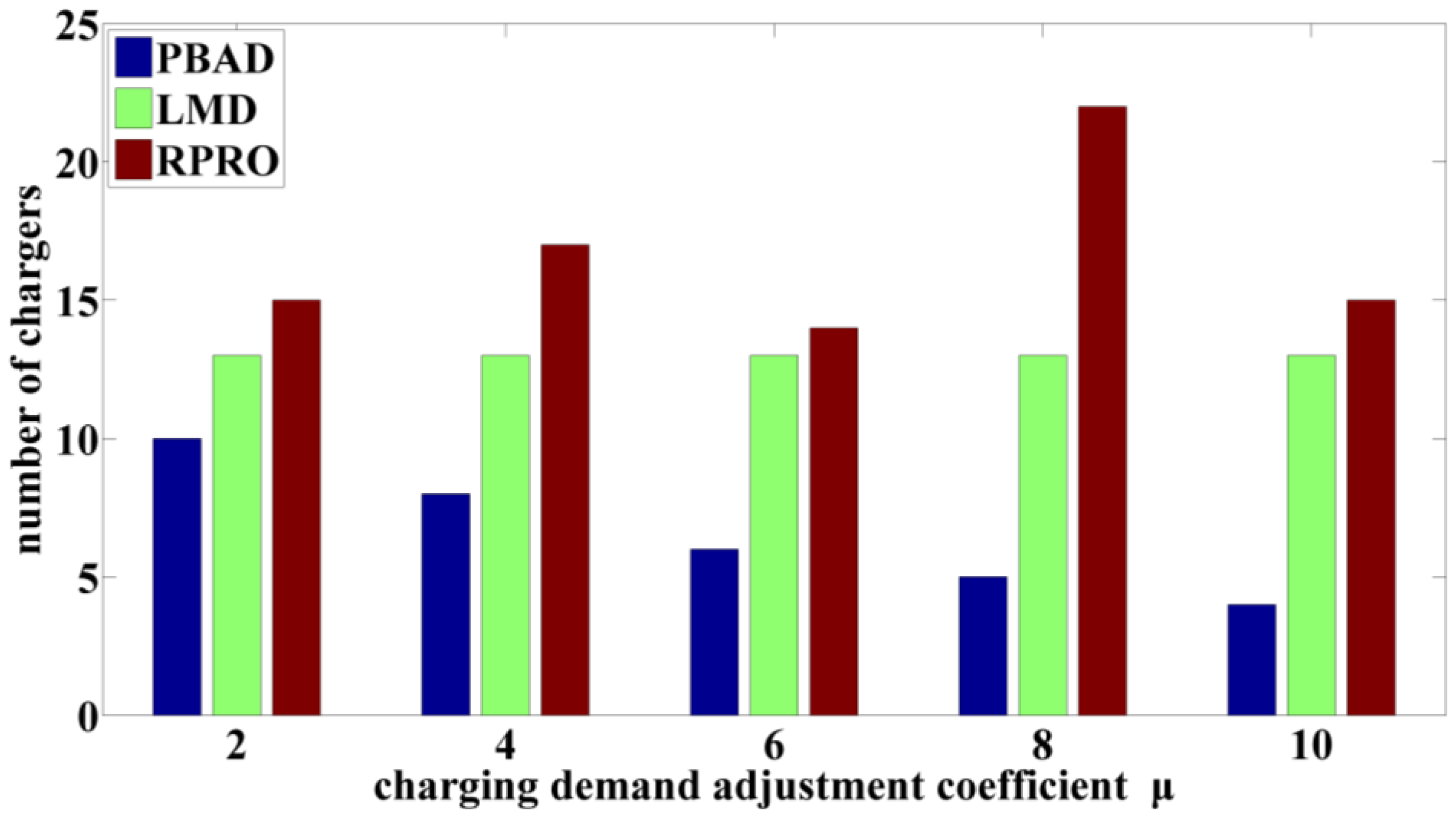
4.2. Effects of the Adjustment Coefficient of Charging Demand μ

This section studies the impact of the charging demand adjustment coefficient on the number of chargers required. We use the results indicated in Section 3.2 as a precondition for the experiment and assume that μ changes within the range of 2 and 10 mW. Figure 10 shows that the LMD algorithm is not affected by μ. This is because the LMD approach does not take the data sink node into account in its deployment. The LMD deployment is meant to maximize the charging power without considering the power balance, so the required number of chargers is always 13. Our deployment method deploys fewer chargers when μ increases, and there is a negative correlation between the number of chargers and μ. This is because the sensor charging demand becomes low. Nevertheless, our method requires less chargers than the LMD method for deployment.

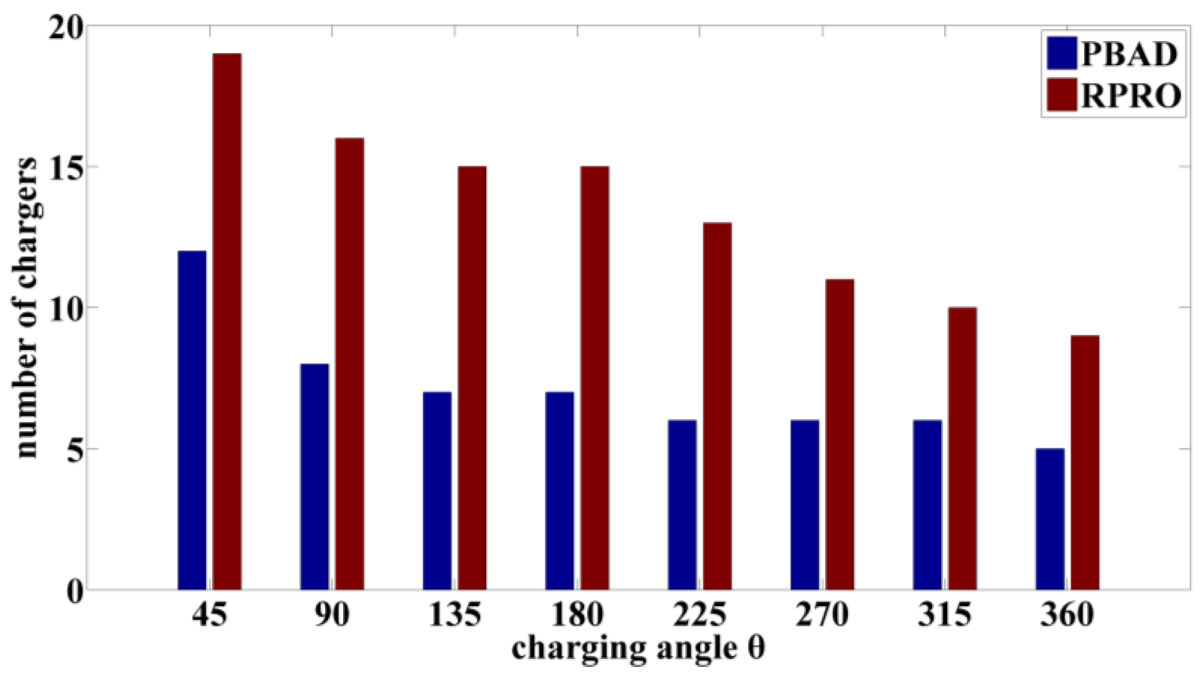
4.3. Effects of the Charging Angle θ

The effects of the charging angle θ on the number of required chargers are explored in this section. The charging angle θ is changed from 40 to 360 degrees. Since LMD can only be applied to the omnidirectional chargers, PBAD is compared with RPRO only in this section. Figure 11 shows that the number of required chargers and the charging angle θ are positive correlated. When the charging angle θ is set to 360 degrees, the deployment results of PBAD can be compared with the results of LMD in Section 3.2. The PBAD deploys 13 chargers less than LMD.

4.4. Charging Efficiency Performance in the Real Case of Each Sensor

In this section, numbers are assigned to the sensors. The closer a sensor is to the data sink node, the smaller the number that is assigned to it. In Figure 12, the effect of the charging efficiency of each sensor in the different algorithms is shown. We limit the number of deployed chargers to 10. The efficiency of the RPRO charging method is very unbalanced; this is because the deployment method randomly picked the interested points. The strategy used by the LMD approach is to find the best charging efficiency for the sensors. In contrast, our method considered the charging demand instead of charging efficiency. The aim of our approach is to maintain the operation of the sensors instead of going after the best charging efficiency. In a realistic environment, our approach can effectively reduce the number of required chargers.

5. Conclusions

In this study, the influence of the data sink node on sensors is considered. Many studies have failed to pay attention to this important factor. This paper takes into account the effect of the data sink node and proposes a power balance aware deployment (PBAD) approach that can reduce the number of the required chargers and still maintain good charging effects. This study considers directional chargers which has been rarely considered among previous studies. The deployment given by the proposed PBAD method can reduce the required number of directional chargers and maintain the charging efficiency. The simulation results show that our approach outperforms the LMD and RPRO approaches by a significant degree and thus further demonstrate the usability of our algorithm.

In a realistic charger deployment, there are still many additional factors that need to be considered, such as charger recharging. It is expected that in the future, more factors can be considered to further optimize the algorithm, so that the charging power can be further improved.

References

1. Pantazis, N.A.; Nikolidakis, S.A.; Vergados, D.D. Energy-efficient routing protocols in wireless sensor networks: A survey. IEEE Commun. Surv. Tutor. 2013, 15, 551–591. [Google Scholar] [CrossRef]
2. Fafoutis, X.; Sørensen, T.; Madsen, J. Energy harvesting—Wireless sensor networks for indoors applications using IEEE 802.11. Procedia. Comput. Sci. 2014, 32, 991–996. [Google Scholar] [CrossRef] [Green Version]
3. Sample, A.P.; Meyer, D.T.; Smith, J.R. Analysis, experimental results, and range adaptation of magnetically coupled resonators for wireless power transfer. IEEE Trans. Ind. Electron. 2010, 58, 544–554. [Google Scholar] [CrossRef]
4. Global Wireless Charging Market 2016–2020. Available online: http://www.prnewswire.com/news-releases/global-wireless-charging-market-2016-2020-300196623.html (accessed on 31 July 2016).
5. Gilbert, D. Wifi Routers can Wirelessly Charge Batteries, Cameras and Sensors. Available online: http://www.ibtimes.co.uk/wifi-routers-can-wirelessly-charge-batteries-cameras-sensors-1504987 (accessed on 31 July 2016).
6. Sendra, S.; Lloret, J.; Garcia, M.; Toledo, J.F. Power saving and energy optimization techniques for wireless sensor neworks. J. Commun. 2011, 6, 439–459. [Google Scholar] [CrossRef]
7. Bri, D.; Garcia, M.; Lloret, J.; Dini, P. Real deployments of wireless sensor networks. In Proceedings of the IEEE Third International Conference on Sensor Technologies and Applications, Athens/Glyfada, Greece, 18–23 June 2009; pp. 415–423.
8. Li, J.; Mohapatra, P. Analytical modeling and mitigation techniques for the energy hole problem in sensor networks. Pervasive Mob. Comput. 2007, 3, 233–254. [Google Scholar] [CrossRef]
9. Lian, J.; Naik, K.; Agnew, G.B. Data capacity improvement of wireless sensor networks using non-uniform sensor distribution. Int. J. Distrib. Sens. Netw. 2006, 2, 121–145. [Google Scholar] [CrossRef]
10. He, S.; Chen, J.; Jiang, F.; Yau, D.K.Y.; Xing, G.; Sun, Y. Energy provisioning in wireless rechargeable sensor networks. IEEE Trans. Mob. Comput. 2013, 12, 1931–1942. [Google Scholar] [CrossRef]
11. Chiu, T.-C.; Shih, Y.-Y.; Pang, A.-C.; Jeng, J.-Y.; Hsiu, P.-C. Mobility-aware charger deployment for wireless rechargeable sensor networks. In Proceedings of the 14th IEEE Asia-Pacific Network Operations and Management Symposium, Seoul, Korea, 25–27 September 2012; pp. 1–7.
12. Liao, J.-H.; Jiang, J.R. Wireless charger deployment optimization for wireless rechargeable sensor networks. In Proceedings of the 7th IEEE International Conference on Ubi-Media Computing, Ulaanbaatar, Mongolia, 12–14 July 2014; pp. 160–164.
13. Horster, E.; Lienhart, R. Approximating optimal visual sensor placement. In Proceedings of the 2006 IEEE International Conference on Multimedia and Expo, Toronto, ON, Canada, 9–12 July 2006; pp. 1257–1260.
14. Han, X.; Cao, X.; Lloyd, E.L.; Shen, C.-C. Deploying directional sensor networks with guaranteed connectivity and coverage. In Proceedings of the 5th Annual IEEE Communications Society Conference on Sensor, Mesh and Ad Hoc Communications and Networks, San Francisco, CA, USA, 16–20 June 2008; pp. 153–160.
15. Fu, L.; Cheng, P.; Gu, Y.; Chen, J.; He, T. Minimizing charging delay in wireless rechargeable sensor networks. In Proceedings of the IEEE INFOCOM 2013, Turin, Italy, 14–19 April 2013; pp. 2922–2930.
16. Garey, M.R.; Johnson, D.S. Computers and Intractibility: A Guide to the Theory of Np-Completeness; W.H. Freeman and Company: New York, NY, USA, 1979. [Google Scholar]
17. Ai, J.; Abouzeid, A.A. Coverage by directional sensors in randomly deployed wireless sensor networks. J. Comb. Optim. 2006, 11, 21–41. [Google Scholar] [CrossRef]
18. Dai, H.; Liu, Y.; Chen, G.; Wu, X.; He, T. Safe charging for wireless power transfer. In Proceedings of the IEEE INFOCOM 2014, Toronto, ON, Canada, 27 April–2 May 2014; pp. 1105–1113.
Figure 1. The power unbalanced phenomenon of wireless sensor networks (WSNs).
Energies 09 00695 g001
Figure 2. Coverage area of a directional charger.
Energies 09 00695 g002
Figure 3. Schematic diagram of the discretization of charging power.
Energies 09 00695 g003
Figure 4. Schematic diagram of regional discretization.
Energies 09 00695 g004
Figure 5. The distribution of the charging demands of the sensors.
Energies 09 00695 g005
Figure 6. A coverage dominating set finding example.
Energies 09 00695 g006
Figure 7. A best dominating set example.
Energies 09 00695 g007
Figure 8. (a) The deployment of PBAD (power balance aware deployment) approach; (b) The deployment of the RPRO (random position and random orientation) approach; (c) The deployment of the LMD (location merging design) approach.
Energies 09 00695 g008
Figure 9. Comparison of charger quantity.
Energies 09 00695 g009
Figure 10. Effects of the charging demand adjustment coefficient μ.
Energies 09 00695 g010
Figure 11. Effects of the angle θ.
Energies 09 00695 g011
Figure 12. (a) Optimal solution; (b) PABD method; (c) LMD method; (d) RPRO method.
Energies 09 00695 g012