
Optimal Power Flow Using the Jaya Algorithm


1
Department of Electrical and Electronic Engineering, Faculty of Engineering, Universiti Putra Malaysia, Serdang 43400, Selangor, Malaysia
2
Centre for Advanced Power and Energy Research, Faculty of Engineering, University Putra Malaysia, Serdang 43400, Selangor, Malaysia
3
Technical Institute Shatra, Southern Technical University, Foundation of Technical Education, Ministry of Higher Education & Scientific Research, Thi-qar 64001, Iraq
*
Author to whom correspondence should be addressed.
Energies 2016, 9(9), 678; https://doi.org/10.3390/en9090678
Submission received: 7 July 2016
/
Revised: 7 August 2016
/
Accepted: 19 August 2016
/
Published: 25 August 2016
(This article belongs to the Special Issue Electric Power Systems Research 2017)
Abstract
:This paper presents application of a new effective metaheuristic optimization method namely, the Jaya algorithm to deal with different optimum power flow (OPF) problems. Unlike other population-based optimization methods, no algorithm-particular controlling parameters are required for this algorithm. In this work, three goal functions are considered for the OPF solution: generation cost minimization, real power loss reduction, and voltage stability improvement. In addition, the effect of distributed generation (DG) is incorporated into the OPF problem using a modified formulation. For best allocation of DG unit(s), a sensitivity-based procedure is introduced. Simulations are carried out on the modified IEEE 30-bus and IEEE 118-bus networks to determine the effectiveness of the Jaya algorithm. The single objective optimization cases are performed both with and without DG. For all considered cases, results demonstrate that Jaya algorithm can produce an optimum solution with rapid convergence. Statistical analysis is also carried out to check the reliability of the Jaya algorithm. The optimal solution obtained by the Jaya algorithm is compared with different stochastic algorithms, and demonstrably outperforms them in terms of solution optimality and solution feasibility, proving its effectiveness and potential. Notably, optimal placement of DGs results in even better solutions.
1. Introduction
Optimum power flow (OPF) solutions are crucial tools in electric power network operation [1,2]. It is an astute power flow that utilizes optimization algorithms to regulate power grid control settings optimally amid diverse constraints [3,4]. Many classical optimization algorithms have been utilized to deal with the OPF problem, like non-linear programming [5,6], the Newton algorithm [7], quadratic programming [8], and decomposition algorithms [9]. A comprehensive review of the deterministic (conventional) optimization algorithms previously employed is presented in [10]. Although these methods can achieve the globally optimal solution in some cases, they have certain shortcomings, such as getting trapped in local optima (i.e., insecure convergence properties), inability to tackle non-differentiable goal functions, and high sensitivity to initial search points. Furthermore, these algorithms cannot guarantee a global solution. Thus, proposing alternative methods to address the above-mentioned drawbacks is a necessity.
The significant development of computers in recent years has resulted in a trend of solving OPF problems using nature-inspired optimization techniques. Various stochastic optimization techniques have been suggested and utilized to deal with OPF problems, like the genetic algorithm [11,12,13], particle swarm optimization (PSO) [2], differential evolution (DE) [14], harmony search (HS) algorithm [15], artificial bee colony algorithm [4,16], gravitational search algorithm (GSA) [17], distributed algorithm (DA) [18], and biogeography-based optimization (BBO) [19,20]. A survey of the non-deterministic search (stochastic search) algorithms utilized to solve variants of OPF is presented in [21]. These algorithms are more efficient in discovering global solutions to different nonlinear OPF problems and are not entangled in local optima. This advantage is achieved through fast and simultaneous evaluation of many points in the solution space. Their universality and the simplicity of implementation make them suitable for large-scale optimization problems. These methods can also handle integer and discrete variables. Unfortunately, regardless of their advantages, each of these population-based optimization algorithms requires appropriately tuned algorithm-specific controlling parameters, because improper tuning of such parameters will raise the computational burden (i.e., affects the convergence property) or leads to a sub-optimal solution.
One of the newly developed population-based optimization methods is the Jaya algorithm, which was proposed by Rao [22] in 2016 to address the aforementioned drawback. Unlike other population-based methods, the optimization procedure of the Jaya algorithm does not involve tuning any algorithm-specific controlling parameters. As mention above, the controlling process of such parameters is not trouble-free. With this feature, a significant benefit of the Jaya algorithm can be achieved in terms of omitting the difficulty of controlling such parameters and decreasing the time necessary for carrying out optimization process. Furthermore, the technique is simple to code and easy to apply. The optimization approach of this technique is inspired by the notion that the solution to a specific problem has to proceed toward the optimum solution and avert inferior ones. Accordingly, one of the main benefits of using the Jaya algorithm is that it has the merit of evading being trapped in local optima, unlike many other population-based optimization algorithms. This notable feature of the Jaya method makes it superior than other population-based optimization methods. In [22], the comparative results of 13 constrained benchmark functions obtained by the Jaya algorithm and many algorithms revealed the superiority of the Jaya algorithm in terms of finding the expected global optimal solutions.
This research was motivated by several factors. First, the application of the Jaya algorithm to solve the optimum power flow problem has not been yet studied. Second, many population-based algorithms produce infeasible solutions for many kinds of OPF problems in terms of violation of operational variables constraints, as reported in [4,20,23]. Lastly, the DG effect when solving the OPF problem using the above-mentioned algorithms has not been examined. Hence, using a powerful optimization algorithm that can effectively solve the OPF problem with and without DG effect is important.
To contribute to the field of OPF solution, the application of the Jaya algorithm to solve different OPF problems is suggested and presented for the first time in this article. The most important contribution is proposing a novel Jaya-based procedure to deal with OPF solution. Furthermore, a modified formulation of the OPF problem which includes DG’s effect is introduced. An extended set of state variables is utilized in the proposed OPF formulation. The set includes active power generation outputs, real power generation of DGs, regulating transformers tap setting, generation node voltage magnitudes, and reactive power injection of shunt capacitors. Three objectives are considered for single optimization in this paper: reduction of generation cost, reduction of real power loss, and voltage stability enhancement. This article also represents a considerable contribution to the field of optimal DG placement in meshed networks, based upon the sensitivity of loss and generation cost to active and reactive power injection.
The modified IEEE 30-bus and IEEE 118-bus networks (i.e., portions of the American electric power system (in the Midwestern US)) are used to examine, validate and exhibit the efficacy of Jaya method. The remainder of this article is arranged as follows: Section 2 presents the proposed mathematical problem formulation for OPF problems that considers the DG effect. Section 3 briefly presents the Jaya algorithm. Section 4 summarizes the application of the Jaya algorithm to the OPF problem. Results, discussion, and comparison with other algorithms are demonstrated in Section 5. Conclusions regarding the implementation of the Jaya algorithm are given in Section 6.
2. Problem Formulation
In this paper, three objectives are selected to deal with the OPF issue with and without incorporating DG effect: minimizing total fuel cost of power generation, real power loss minimization, and voltage stability improvement. The total fuel cost of a specified power network is represented by the following function:
where NG is the number of generation units, whereas fi represent the fuel cost of the i-th generation unit that can be expressed by quadratic function as follows:
where ai, bi, and ci represent the fuel cost coefficients of the i-th generation unit, whereas PGi is the active power output of the ith generator. Meanwhile, the total system active power losses Ploss can be defined as:
where N is the number of network nodes; Vi and Vj are the voltage magnitudes for the i-th and j-th nodes, respectively; δi and δj are the node voltage angles of the i-th–j-th branch; and Gij refers to the conductivity between node i and node j.
The voltage stability of a particular power grid can be assessed using the widely utilized indicator, L-index, that is, Lmax [24]:
where Lk is the L-index of the kth load bus and NL is the number of load buses.
Additionally, the optimization of the real power generation of DG units is another target toward achieving a superior solution to the OPF problem. Hence, DGs optimum penetration has been incorporated into the suggested formulation as an additional control variable. Mathematically, the proposed formulation of OPF problem that considers DG can be expressed as:
subject to:
- a
- Equality constraints which stand for load flow equationsin polar form:
- b
- Inequality constraints that represent the control variable constraints:
The modified vector of control variables that considers the real power generation of DGs can be stated as:
where PG refers to the active power generation outputs with the exception of swing bus, Ti is the tapping ratio of the i-th transformer, VGi is the voltage magnitude of the unit i, QCi is the imaginary power injection by the i-th shunt capacitor, PDGi is the real power generation of the i-th DG unit, NG is the number of generator buses, NT is the number of tap changing transformers, NC is the number of shunt capacitors, and NDG is the number of DG units.
- c
- Inequality constraints that comprise the dependent variable constraints.
The developed version of the vector of dependent variables that considers the reactive power generation of DG units can be defined as:
where PSlack is the active power of the slack bus, VLi is the voltage of i-th load node, Sline,i is the loading of the i-th transmission line, QDGi is the imaginary power generation of the i-th DG unit, NL is the number of load buses, and Nl is the number of transmission lines.
The literature shows several approaches to handling dependent variable constraints in population-based optimization algorithms. One efficient approach is to incorporate these constraints into the goal function as quadratic penalty expressions (i.e., the penalty factor method). Each term added to the goal function comprises a given penalty factor multiplied by the square of the violated value of a dependent variable. Consequently, any obtained infeasible candidate solution is denied. In this work, the modified goal function includes quadratic penalty terms of the extended set of dependent variables (i.e., PSlack, VL, QG, Sline, and QDG). Notably, a quadratic penalty term for the reactive power of DG is added. The mathematical formulation of the modified i-th goal function can be stated as follows:
where Fi is the i-th goal function to be optimized, is the i-th modified goal function, and λP, λV, λO, λS and λDG are the penalty factors which can be assigned subjectively by a decision maker. Normally, using high penalties is desirable to insure that any infeasible solution is declined. xlim is the upper/lower bound value of the dependent variable x that can be stated in the following formulation:
It is worth mentioning that the above mathematical formulation of the modified goal function is just used in case a dependent variable(s) violates the upper/lower limit. The main aim is to detect and avoid any discovered infeasible solution(s) during the optimization process. Notably, the choice of the penalty terms (λP, λV, λO, λS and λDG) play a crucial role. Based on application and designer experience, the penalty terms may be different for different boundaries. Using of different penalty factors lead to different solutions. To address this issue, a high unity penalty of 10000 has been considered in this paper for each dependent variables in case of violation the upper/lower limit. However, it would be desirable to update the penalty terms in the objective function dynamically in the algorithm.
3. The Jaya Algorithm
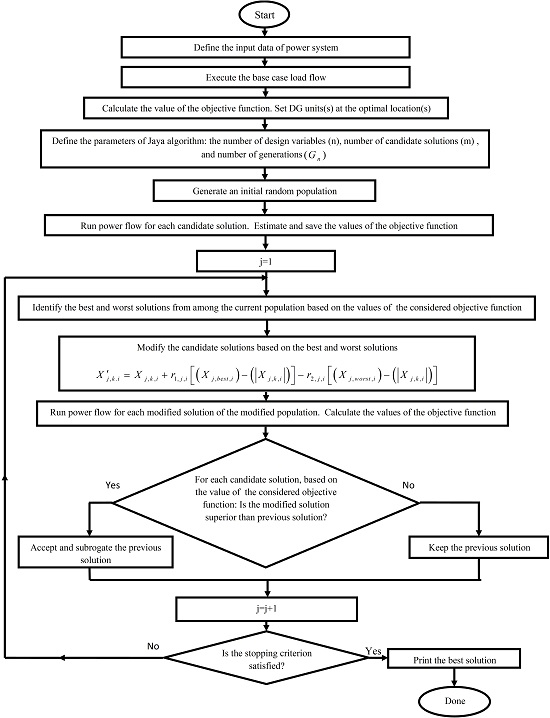
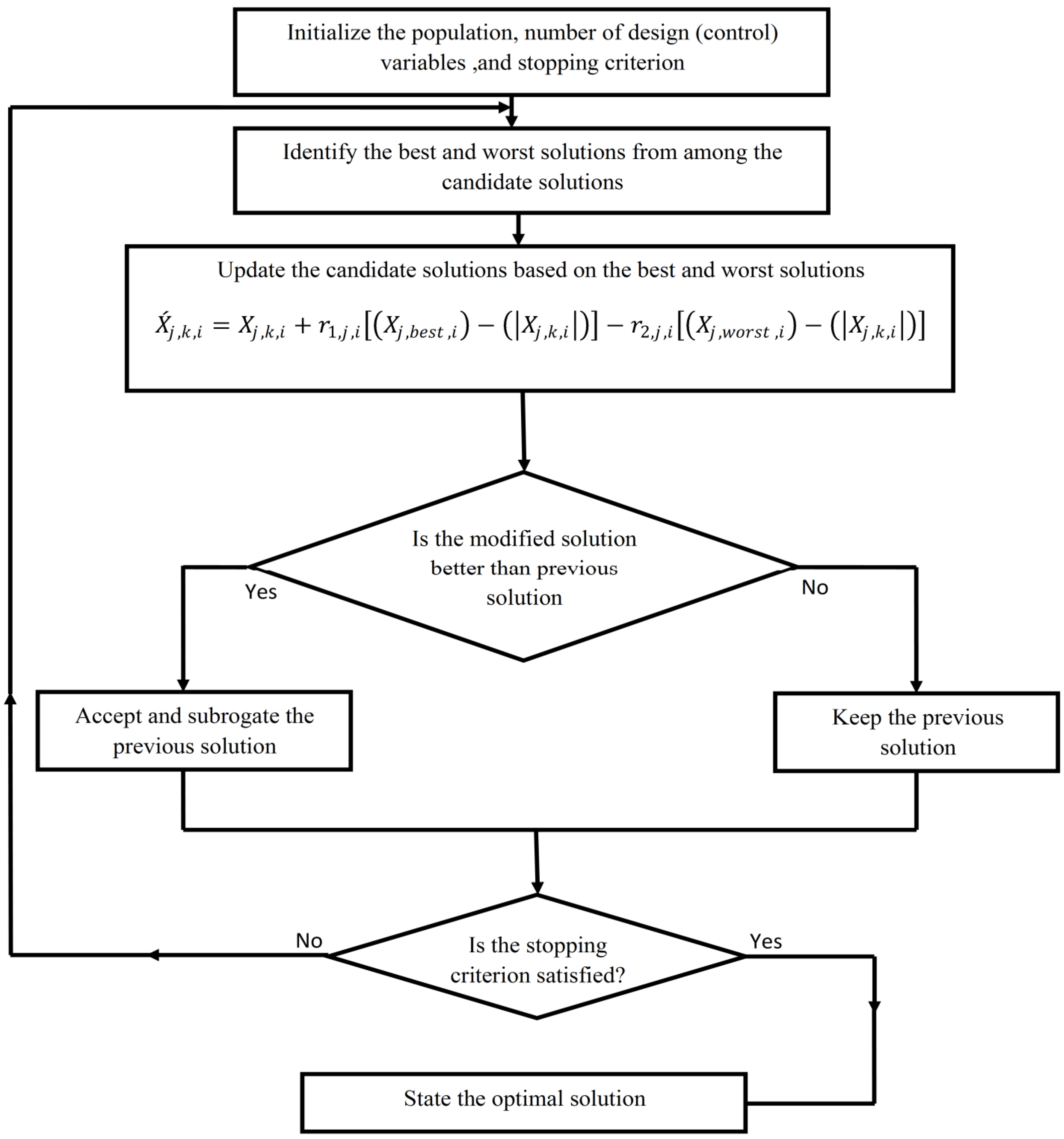
Jaya is a new population-based optimization algorithm introduced by Rao [22] to produce optimal solutions for constrained and unconstrained optimization problems. Unlike other population-based heuristic algorithms, Jaya has no algorithm-specific controlling parameter, and involves only the two ordinary controlling parameters of population size (m) (that is, the number of candidate solutions) and the number of generations (Gn) (that is, the total iterations). The optimization process of this technique is elicited on the basis of the idea that the solution determined for a specific problem have to shift toward the optimum solution and evade the inferior solution [22]. The basic Jaya algorithm has only one phase according to the aforementioned concept, making it a simple optimization technique. Figure 1 illustrates the flowchart of Jaya algorithm.
4. Application of Jaya Algorithm to OPF Problem
The following steps describe the proposed process of applying the Jaya algorithm to solve the OPF problem:
- Step 1
- Define the branch data, active and reactive power load levels, and generation units data. Specify the initial values of active power generation of PV buses, real power production of the DGs (in case of considering DG), reactive power injection for shunt compensators, voltage magnitudes of generation buses, and the tap setting of regulating transformers.
- Step 2
- Run the initial status load dispatch. Calculate the values of the goal functions for the initial status, that comprise generation cost reduction, real power loss reduction, and voltage stability improvement, using Equations (1), (3), and (4) , respectively.
- Step 3
- Allocate the DG unit(s) to suitable site(s) on the basis of the sensitivity of active power loss and generation cost to both active and reactive power injection as stated in the following formulations:
- Step 4
- Define the i-th objective function Fi(x,u) to be optimized (that is one of the objective functions described in Section 2). Initialize the number of control (design) variables (n), population size (m) (that is, the number of candidate solutions), number of iterations (Gn), and minimum and maximum limits of design variables (UL, LL).
- Step 5
- Create an initial random population based on the defined controlling parameters within the pre-specified limits of design variables. This population is formulated as follows:
- Step 6
- Run power flow program for each candidate solution and calculate the value of goal function that corresponds to each solution.
- Step 7
- Identify the best and worst solutions among the candidate solutions.
- Step 8
- Based on the best and worst solutions, modify all candidate solutions. The proposed modification is expressed as follows:
Throughout the ith iteration (generation) and for each kth candidate solution, the value of the jth design variable (Xj,k,i) can be modified as follows [22]:
where is the modified value of the j-th design variable, and are randomly generated numbers within the range of (0–1) for the j-th control variable. is the value of the j-th design variable for the top nominee solution. is the value of the j-th design variable for the inferior nominee solution. The second term of the above equation stand for the propensity of the modified solution to proceed closer to the optimum solution. The third expression stands for the propensity of the solution to eschew the worst solution.
- Step 9
- For all updated solutions, if any control variable upper/lower limit is violated, replace the estimated value with the corresponding limit.
- Step 10
- Execute the power dispatch considering the modified vector of design variables. Calculate the new values of the goal function and distributed generation size for each candidate solution. Add the assigned penalty(s) to the value of the goal function in case a dependent variable(s) violates the upper/lower limit, using Equation (20).
- Step 11
- For each candidate solution, compare the objective function Fi(x,u) values for the previous and updated solution. Accept the updated solution if it is superior to the previous solution. Otherwise, keep the previous solution.
- Step 12
- Stop and report the optimal solution if the termination criterion is achieved. Otherwise, return to step 7.
For more explanation, the flowchart of the proposed application of Jaya algorithm to solve OPF problem is shown in Figure 2.
5. Results and Discussion
To examine the efficacy of the Jaya algorithm for single OPF problems considering DG, the algorithm is implemented in the IEEE 30-bus network and the IEEE 118-bus network. For the IEEE 30-bus network, the population size (m) and maximal number of generation (Gn) are set to 40 and 100, respectively. The case considered for the IEEE 118-bus network is carried out with a population size (m = 100) and a maximum of 300 iterations. The Jaya algorithm is performed in the computational environment of MATLAB R2015b [26] and implemented on a PC with a 2.7 GHz Intel® Core™ (Intel Corporation, 2200 Mission College Blvd.: Santa Clara, CA, USA) i7 CPU and 16 GB RAM.
5.1. IEEE 30-Bus Network
The essential data of this network is shown in [27]. The network has six generator units at buses 1, 2, 5, 8, 11, and 13. Load buses 10, 12, 15, 17, 20, 21, 23, 24, and 29 are equipped with switchable shunt capacitors. Four tap changing transformers are installed at lines 6–9, 6–10, 4–12, and 27–28. The voltage level bounds of all load buses are set to (0.95, 1.05) p.u. A prevalent DG unit which can produce active and reactive power is also utilized throughout the implementation of Jaya algorithm, with a 10 MW generation capability and 0.8 power factor. According to the results obtained from Equations (22) and (23), we found that bus number 30 is the nominee location for DGs accommodation with the top sensitivities of active power loss and generation cost to each of active and reactive power injection, that are (−0.1408), (−0.0516), (−0.0926), and (−0.0383), respectively. We noticed that bus 3 is the worst location, because it had the least sensitivities of active power loss and generation cost to both injected active and reactive powers, which are (−0.0362), (0.007), (−0.0208), and (−0.001).
Accordingly, the aforementioned locations are used for DG accommodation throughout the implementation of the Jaya method for single optimization cases. The representative single-line digram of this network that contains all the required measures in the Jaya algorithm is illustrated in Figure 3.
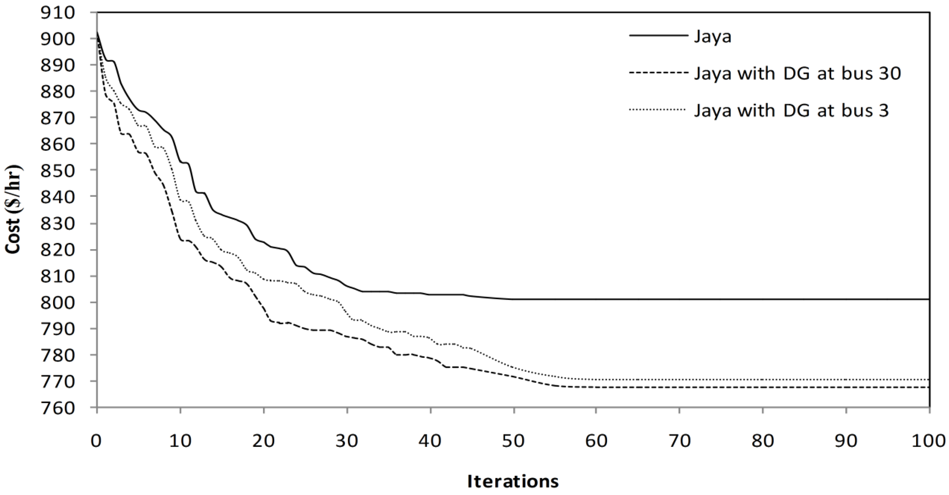
5.1.1. Case 1: Fuel Cost Minimization
In this section, fuel cost minimization is considered the goal function during the implementation of Jaya algorithm with and without the influence of DG. Figure 4 illustrates the convergence graph of fuel cost minimization using the Jaya algorithm with and without incorporating the distributed generation unit at nodes 30 and 3. Without considering DG’s effect, the method requires 49 iterations to obtain the optimum solution, which reveals the excellent convergence rate of the Jaya algorithm. The best adjustments of the design variables and optimal values of cost minimization are tabulated in Table 1. The results present a significant reduction in fuel cost from 902.0207 $/h to 800.4794 $/h, when the Jaya algorithm is executed without considering DG. In addition, the average computational time for single iteration for this case is 0.724 s. These results point out the effectiveness of the Jaya algorithm in terms of solution optimality and fast convergence. Fuel cost is compared with that obtained using various other heuristic optimization algorithms to validate the Jaya algorithm further. Table 2 demonstrates the supremacy of the Jaya algorithm over previous algorithms. Notably, the majority of obtained solutions using heuristic optimization algorithms (Table 2) are infeasible, which is principally due to voltage magnitude violations at one or more system load buses, as well as reactive power generation bound violations at one or more generation units. Notably, [23] also reported solution infeasibility for many previous methods, as compared in Table 2. Implementing Jaya method for fuel cost reduction when accommodating the DG at node 30 produces an even more significant reduction in fuel cost, reaching 768.0398 $/h, an attractive Lmax value (0.0969), and a great expansion of shunt compensators reactive power saving of up to 29.8391 MVAR. Most importantly, a considerable reduction in active power losses (8.4983 MW) is achieved. Additionally, as a worst site for DG accommodation, node 3 leads to a critical rise of 12.804% in the L-index that results in a slight decrease of 0.812% in losses as compared with the results gained for cost optimization without utilizing DG. These findings exhibit the superiority of the Jaya algorithm over several heuristics techniques for solving this type of problem, and reinforce the efficacy of the proposed DG placement technique.
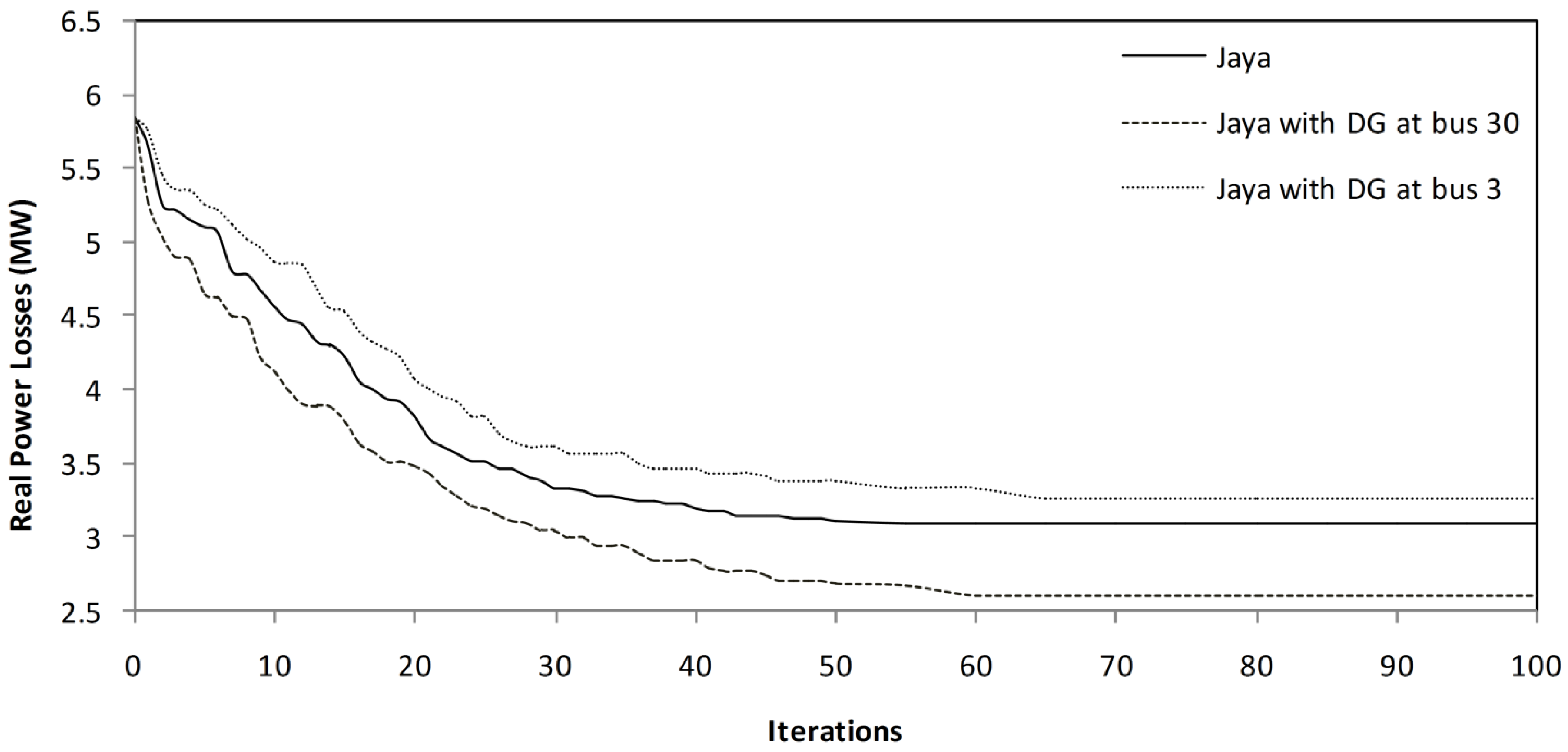
5.1.2. Case 2: Real Power Losses Reduction
The goal considered in this case was active power losses minimization. The Jaya algorithm was utilized to attain the optimum solution, the results of which are given in Table 1. The Jaya algorithm is clearly efficient for determining the optimum settings of the control variable, which minimizes system losses. Consequently, real power losses is decreased significantly from 5.8482 MW to 3.1035 MW when Jaya algorithm is performed without considering DG. Figure 5 shows the steep convergence of real power losses using the Jaya algorithm while considering DG placement at buses 30 and 3.
The algorithm fully reaches to the optimum solution with 65 iterations, demonstrating the rapid convergence of the Jaya algorithm. To test the effectiveness of the algorithm, estimated real power loss value is compared with that obtained using previously reported population-based optimization algorithms. Table 3 illustrates the superiority of the Jaya algorithm over these earlier algorithms. The solution obtained using HS [15] algorithm (Table 3) is infeasible because of the voltage magnitude violations at all load buses except bus 7 (Adaryani et al. have also reported this issue) [4].
Implementing the Jaya method for loss minimization when placing the DG at the best site leads to further minimization (2.675040 MW), a considerable saving in generation cost (46.0839 $/h) accompanied by an excellent voltage stability index value (0.0892). Furthermore, the shunt compensator reserve margin increases extensively by 110.787%. In contrast, placing a DG at node 3 (that is, the worst node for DG accommodation) while executing the OPF solution minimizes losses to 3.339 MW. This result is inferior when compared with loss minimization that does not utilize DG, which is 3.1035 MW. A critical increment of 11.871% Lmax is also obtained. The findings confirm that optimal placement of DG leads to a superior solution to the OPF problem. To sum up, these findings validate the supremacy of the Jaya algorithm over other techniques reported in the literature, both in terms of solution optimality and feasibility.
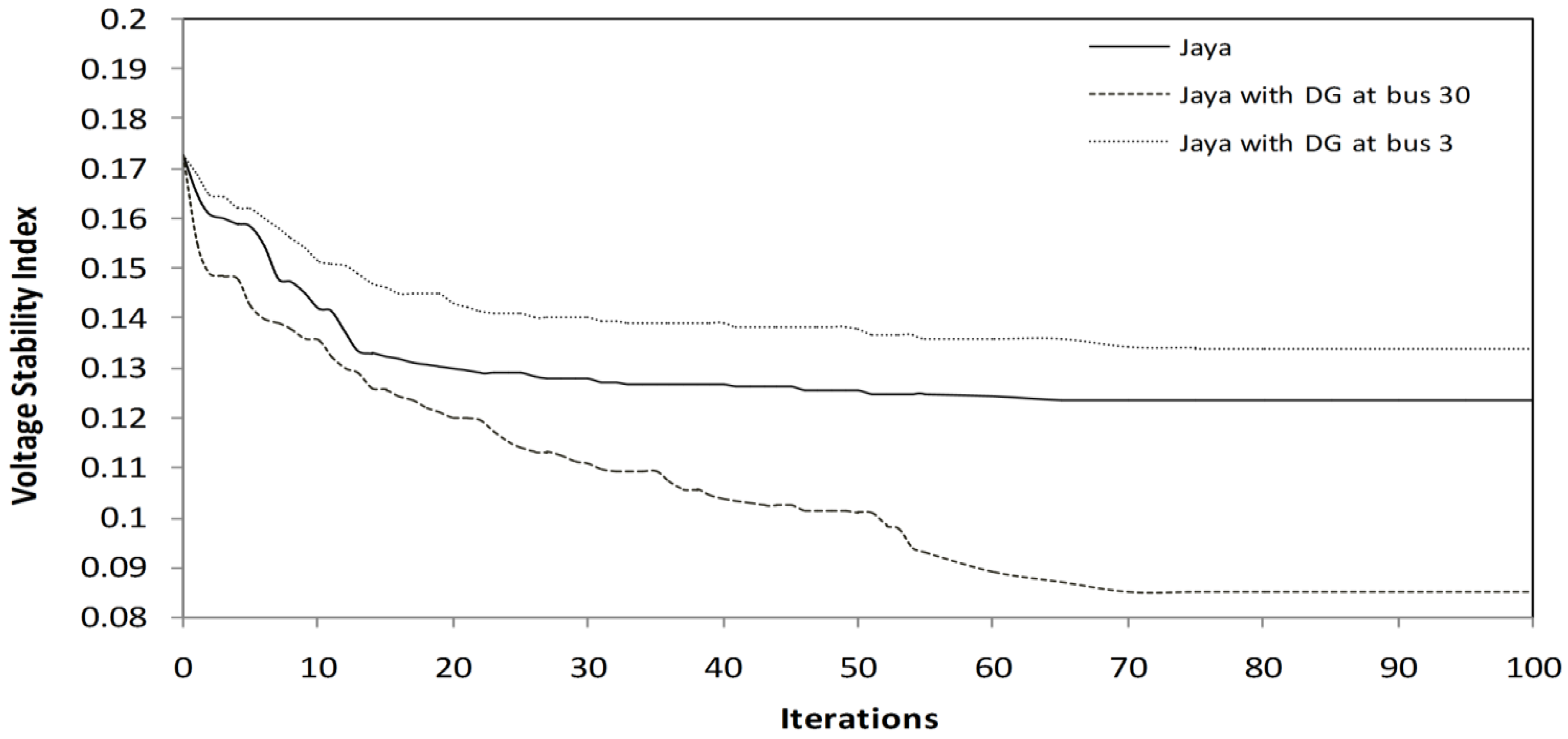
5.1.3. Case 3: Voltage Stability Improvement
In this section, enhancing voltage stability is selected as the goal function to be optimized using the Jaya algorithm while considering the effects of DG placement. The trend of enhancing system voltage stability is sketched in Figure 6. The results are given in Table 1. The findings point out that the voltage stability index is reinforced by 28.23%. Table 4 compares solutions achieved using Jaya method and other population-based optimization techniques, with the former yielding clearly superior results. Remarkably, placing a DG unit at bus 30 while executing OPF significantly reduces Lmax index to 0.0851, whereas integrating a DG unit at the worst location (i.e., bus 3) increases Lmax index to 0.1371.
5.1.4. Statistical Analysis
A statistical study is performed to examine the robustness and efficacy of the Jaya algorithm in solving OPF problems that considers DG effect. For each case, 50 independent trials of the Jaya algorithm with different initial populations (solutions) are carried out. As previously mentioned, for the modified IEEE 30-bus test network, population size (m) and utmost number of generation (Gn) are set to 40 and 100, respectively. In this paper, the statistical analysis indices employed are best value, worst value, average (mean) value, and standard variation (SD). Statistical analysis results are presented in Table 5. The table presents that the best, worst, and average values for all considered cases are very close to each other; hence the standard deviation values were small. These results affirm the robustness of the Jaya algorithm and its capability to explore the optimal solution in every run.
5.2. IEEE 118-Bus Network
The standard IEEE 118-bus network is considered to verify the scalability and efficacy of the Jaya algorithm for solving large-scale OPF problems. The complete data of this system are referenced in [33]. The network has 186 branches, 54 generating units, and 64 load buses. Twelve buses, 34, 44, 45, 46, 48, 74, 79, 82, 83, 105, 107, and 110 are equipped with switchable shunt capacitors. Meanwhile, nine tap changing transformers are installed at lines 8–5, 26–25, 30–17, 38–37, 63–59, 64–61, 65–66, 68–69, and 81–80. The voltage magnitude limits of all buses are set within the range of [0.95 p.u., 1.1 p.u.]. The minimum and maximum limits for each regulating transformer tap are within the domain of (0.9, 1.1). The imaginary power inserted by each shunt capacitor is set within the range of [0 MVAR, 30 MVAR].
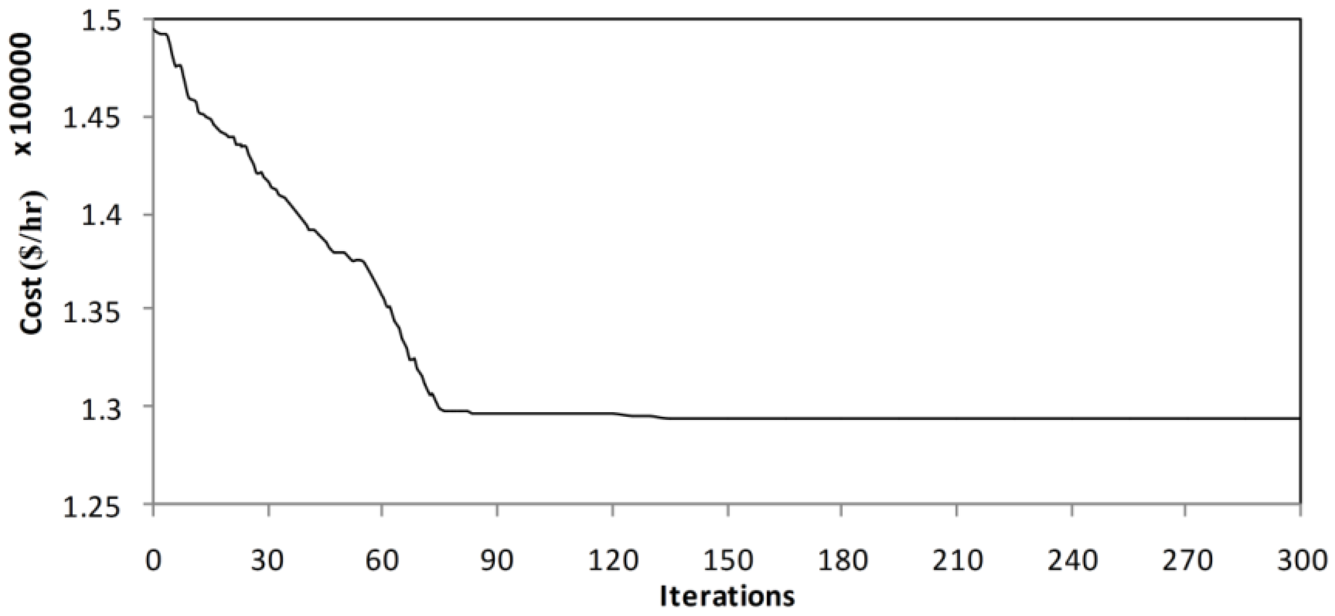
Case 4: Fuel Cost Reduction
In this section, the Jaya algorithm is used to solve the OPF problem of IEEE 118-bus network with cost reduction as the goal function without DG. The convergence graph of Jaya algorithm for cost reduction is sketched in Figure 7.
The figure exhibits the excellent convergence property of Jaya algorithm when solving a large-scale optimization problem. Remarkably, the average computational time of one iteration for this case is 1.83 s. The optimal adjustments of control variables and optimal values of cost minimization are tabulated in Table 6.
For further validation, the results obtained with Jaya algorithm are compared with those of TLBO [28], GSA [34], BBO [34], PSO [35], DE [36], and GWO [36], as shown in Table 7. Jaya algorithm obviously obtained a more superior solution. The findings demonstrate the superiority of Jaya approach in achieving the optimal solution with fast convergence. In total, these results affirm the scalability of the Jaya algorithm and exhibit its efficacy for solving large-scale OPF problems.
6. Conclusions
In this article, a new optimization algorithm, namely the Jaya algorithm, is employed and successfully applied to deal with the OPF problem in electric power networks. Unlike other population-based techniques, this technique does not need controlling factors to be tuned. The algorithm is entered into the OPF problem formulation without and with considering distributed generation. Furthermore, a new formulation of the OPF problem that considers the effect of DG utilization is introduced. A sensitivity based-method is also modified to recognize the optimal placement of DG. Generation cost reduction, active power losses reduction, and voltage stability improvement are goal functions considered for the OPF problem. Standard IEEE 30-bus and IEEE 118-bus networks were utilized to test and validate the applicability of Jaya method in solving OPF problems. Results showed that an optimal and feasible solution for each considered case could be determined by the Jaya algorithm. In fact, the new proposed concept of the Jaya algorithm led to rapid discovery of an optimal solution (that is, strengthened the exploration property). Moreover, results indicated the efficacy of Jaya algorithm in terms of the favorable convergence characteristic and short computation time. Statistical analysis confirmed that Jaya algorithm is a robust optimization technique. For further validation, the performance of Jaya algorithm was compared with existing methods stated in literature. The supremacy of Jaya algorithm was revealed in term of solution optimality and solution feasibility. In fact, the victorious concept of Jaya method makes it superior than other population-based optimization methods. Moreover, the optimal placement of DG units in terms of generation cost and power loss sensitivities, together with the Jaya algorithm approach, led to better solution for all single objective optimization cases. The erroneous placement of DG resulted in unattractive solutions. In conclusion, the applicability, potential, and efficacy of the Jaya algorithm in solving OPF problems for small and large-scale power systems were confirmed. Jaya algorithm is a powerful tool for solving such problems and is a good candidate for solving OPF problems of practical power systems. In the future, the performance of the Jaya algorithm can be compared with other global solvers exist which can guarantee global optimality such as Lindoglobal, Antigone and Baron.
Acknowledgments
The authors gratefully acknowledge the University Putra Malaysia, Faculty of Engineering, Department of Electrical and Electronic Engineering, for providing the necessary facilities. The author Warid Warid would like to thank the Iraqi Ministry of Higher Education & Scientific Research, Foundation of Technical Education, Southern Technical University and Technical Institute Shatra for the unceasing encouragement, support and attention.
Author Contributions
Warid Warid, Hashim Hizam, Norman Mariun, and Noor Izzri Abdul-Wahab conceived and designed the experiments; Warid Warid performed the experiments, analyzed the data, contributed materials/analysis tools, established and validated the models and wrote the paper. Hashim Hizam, Norman Mariun and Noor Izzri Abdul-Wahab provided ideas for the discussion; Warid Warid, Hashim Hizam, Norman Mariun, and Noor Izzri Abdul-Wahab reviewed the article.
Conflicts of Interest
The authors declare no conflict of interest.
References
- Zhu, J. Optimal power flow. In Optimization of Power System Operation, 2nd ed.; John Wiley & Sons, Inc.: Hoboken, NJ, USA, 2009. [Google Scholar]
- Abido, M.A. Optimal power flow using particle swarm optimization. Int. J. Electr. Power Energy Syst. 2002, 24, 563–571. [Google Scholar] [CrossRef]
- Kumar, S.; Chaturvedi, D.K. Optimal power flow solution using fuzzy evolutionary and swarm optimization. Int. J. Electr. Power Energy Syst. 2013, 47, 416–423. [Google Scholar] [CrossRef]
- Adaryani, M.R.; Karami, A. Artificial bee colony algorithm for solving multi-objective optimal power flow problem. Int. J. Electr. Power Energy Syst. 2013, 53, 219–230. [Google Scholar] [CrossRef]
- Dommel, H.W.; Tinney, W.F. Optimal power flow solution. IEEE Trans. Power App. Syst. 1968, 87, 1866–1876. [Google Scholar] [CrossRef]
- Alsac, O.; Stott, B. Optimal load flow with steady-state security. IEEE Trans. Power App. Syst. 1968, 93, 745–751. [Google Scholar] [CrossRef]
- Sun, D.I.; Ashley, B.; Brewer, B.; Hughes, A.; Tinney, W.F. Optimal power flow by Newton approach. IEEE Trans. Power App. Syst. 1984, 103, 2864–2880. [Google Scholar] [CrossRef]
- Burchett, R.C.; Happ, H.H.; Vierath, D.R. Quadratically convergent optimal power flow. IEEE Trans. Power App. Syst. 1984, 103, 3267–3275. [Google Scholar] [CrossRef]
- Shoults, R.R.; Sun, D.T. Optimal power flow based upon P-Q decomposition. IEEE Trans. Power App. Syst. 1982, 101, 397–405. [Google Scholar] [CrossRef]
- Frank, S.; Steponavice, I.; Rebennack, S. Optimal power flow: a bibliographic survey I Formulations and deterministic methods. Energy Syst. 2012, 3, 221–258. [Google Scholar] [CrossRef]
- Lai, L.L.; Ma, J.T.; Yokoyama, R.; Zhao, M. Improved genetic algorithms for optimal power flow under both normal and contingent operation states. Int. J. Electr. Power Energy Syst. 1997, 19, 287–292. [Google Scholar] [CrossRef]
- Bakirtzis, A.G.; Biskas, P.N.; Zoumas, C.E.; Petridis, V. Optimal power flow by enhanced genetic algorithm. IEEE Trans. Power Syst. 2002, 17, 229–236. [Google Scholar] [CrossRef]
- Kumari, M.S.; Maheswarapu, S. Enhanced Genetic Algorithm based computation technique for multi-objective Optimal Power Flow solution. Int. J. Electr. Power Energy Syst. 2010, 32, 736–742. [Google Scholar] [CrossRef]
- Abou El Ela, A.A.; Abido, M.A.; Spea, S.R. Optimal power flow using differential evolution algorithm. Electr. Power Syst. Res. 2010, 80, 878–885. [Google Scholar] [CrossRef]
- Sivasubramani, S.; Swarup, K.S. Multi-objective harmony search algorithm for optimal power flow problem. Int. J. Electr. Power Energy Syst. 2011, 33, 745–752. [Google Scholar] [CrossRef]
- He, X.; Wang, W.; Jiang, J.; Xu, L. An improved artificial bee colony algorithm and its application to multi-objective optimal power flow. Energies 2015, 8, 2412–2437. [Google Scholar] [CrossRef]
- Duman, S.; Güvenç, U.; Sönmez, Y.; Yörükeren, N. Optimal power flow using gravitational search algorithm. Energy Conv. Manag. 2012, 59, 86–95. [Google Scholar] [CrossRef]
- Sanseverino, E.; di Silvestre, M.; Badalamenti, R.; Nguyen, N.; Guerrero, J.; Meng, L. Optimal power flow in islanded microgrids using a simple distributed algorithm. Energies 2015, 8, 11493–11514. [Google Scholar] [CrossRef] [Green Version]
- Bhattacharya, A.; Chattopadhyay, P.K. Application of biogeography-based optimisation to solve different optimal power flow problems. IET Gener. Trans. Distrib. 2011, 5, 70–80. [Google Scholar] [CrossRef]
- Christy, A.A.; Raj, P.A.D.V. Adaptive biogeography based predator–prey optimization technique for optimal power flow. Int. J. Electr. Power Energy Syst. 2014, 62, 344–352. [Google Scholar] [CrossRef]
- Frank, S.; Steponavice, I.; Rebennack, S. Optimal power flow: a bibliographic survey II Non-deterministic and hybrid methods. Energy Syst. 2012, 3, 259–289. [Google Scholar] [CrossRef]
- Rao, R. Jaya: A simple and new optimization algorithm for solving constrained and unconstrained optimization problems. Int. J. Ind. Eng. Comput. 2016, 7, 19–34. [Google Scholar]
- Radosavljević, J.; Klimenta, D.; Jevtić, M.; Arsić, N. Optimal power flow using a hybrid optimization algorithm of particle swarm optimization and gravitational search algorithm. Electr. Power Compon. Syst. 2015, 43, 1958–1970. [Google Scholar] [CrossRef]
- Thukaram, B.D.; Parthasarathy, K. Optimal reactive power dispatch algorithm for voltage stability improvement. Int. J. Electr. Power Energy Syst. 1996, 18, 461–468. [Google Scholar] [CrossRef]
- Frank, S.; Rebennack, S. An introduction to optimal power flow: Theory, Formulation, and Examples. IIE Trans. 2016. [Google Scholar] [CrossRef]
- MATLAB Release R2015b; The MathWorks, Inc.: Natick, MA, USA.
- Lee, K.Y.; Park, Y.M.; Ortiz, J.L. A united approach to optimal real and reactive power dispatch. IEEE Trans. Power App. Syst. 1985, 104, 1147–1153. [Google Scholar] [CrossRef]
- Bouchekara, H.R.E.H.; Abido, M.A.; Boucherma, M. Optimal power flow using Teaching-Learning-Based Optimization technique. Electr. Power Syst. Res. 2014, 114, 49–59. [Google Scholar] [CrossRef]
- Ghasemi, M.; Ghavidel, S.; Gitizadeh, M.; Akbari, E. An improved teaching–learning-based optimization algorithm using Lévy mutation strategy for non-smooth optimal power flow. Int. J. Electr. Power Energy Syst. 2015, 65, 375–384. [Google Scholar] [CrossRef]
- Younes, M.; Khodja, F.; Kherfane, R.L. Multi-objective economic emission dispatch solution using hybrid ffa (firefly algorithm) and considering wind power penetration. Energy 2014, 67, 595–606. [Google Scholar] [CrossRef]
- Attia, A.-F.; Al-Turki, Y.A.; Abusorrah, A.M. Optimal power flow using adapted genetic algorithm with adjusting population size. Electr. Power Compon. Syst. 2012, 40, 1285–1299. [Google Scholar] [CrossRef]
- Abido, M.A. Multiobjective optimal power flow using strength Pareto evolutionary algorithm. In Proceedings of the Universities Power Engineering Conference (UPEC), Bristol, UK, 8 September 2004; pp. 457–461.
- The IEEE 118-Bus Test System. Available online: http://www.ee.washington.edu/research/pstca/pg_tca118bus.html (accessed on 12 April 2016).
- Bhattacharya, A.; Roy, P.K. Solution of multi-objective optimal power flow using gravitational search algorithm. IET Gener. Trans. Distrib. 2012, 6, 751–763. [Google Scholar] [CrossRef]
- Hinojosa, V.H.; Araya, R. Modeling a mixed-integerbinary small-population evolutionary particle swarm algorithm for solving the optimal power flow problem in electric power systems. Appli. Soft Comput. 2013, 13, 3839–3852. [Google Scholar] [CrossRef]
- El-Fergany, A.A.; Hasanien, H.M. Single and multi-objective optimal power flow using Grey Wolf Optimizer and Differential Evolution Algorithms. Electr. Power Compon. Syst. 2015, 43, 1548–1559. [Google Scholar] [CrossRef]
Figure 1.
Flowchart demonstrating the optimization process of the basic Jaya algorithm [22].
Figure 1.
Flowchart demonstrating the optimization process of the basic Jaya algorithm [22].

Figure 2.
Flowchart of the application of Jaya algorithm for the OPF problem.
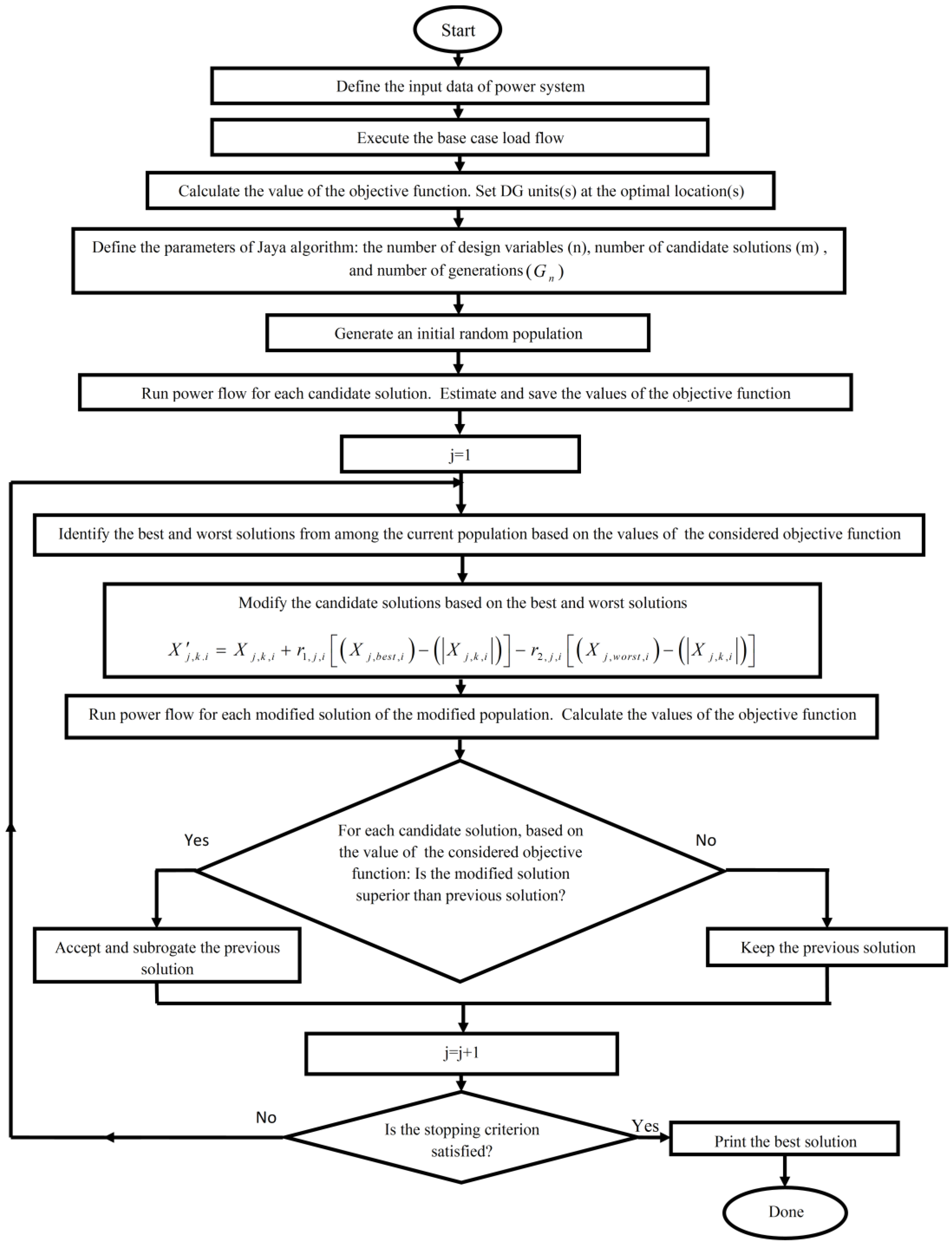
Figure 3.
One line diagram of IEEE 30-bus network.
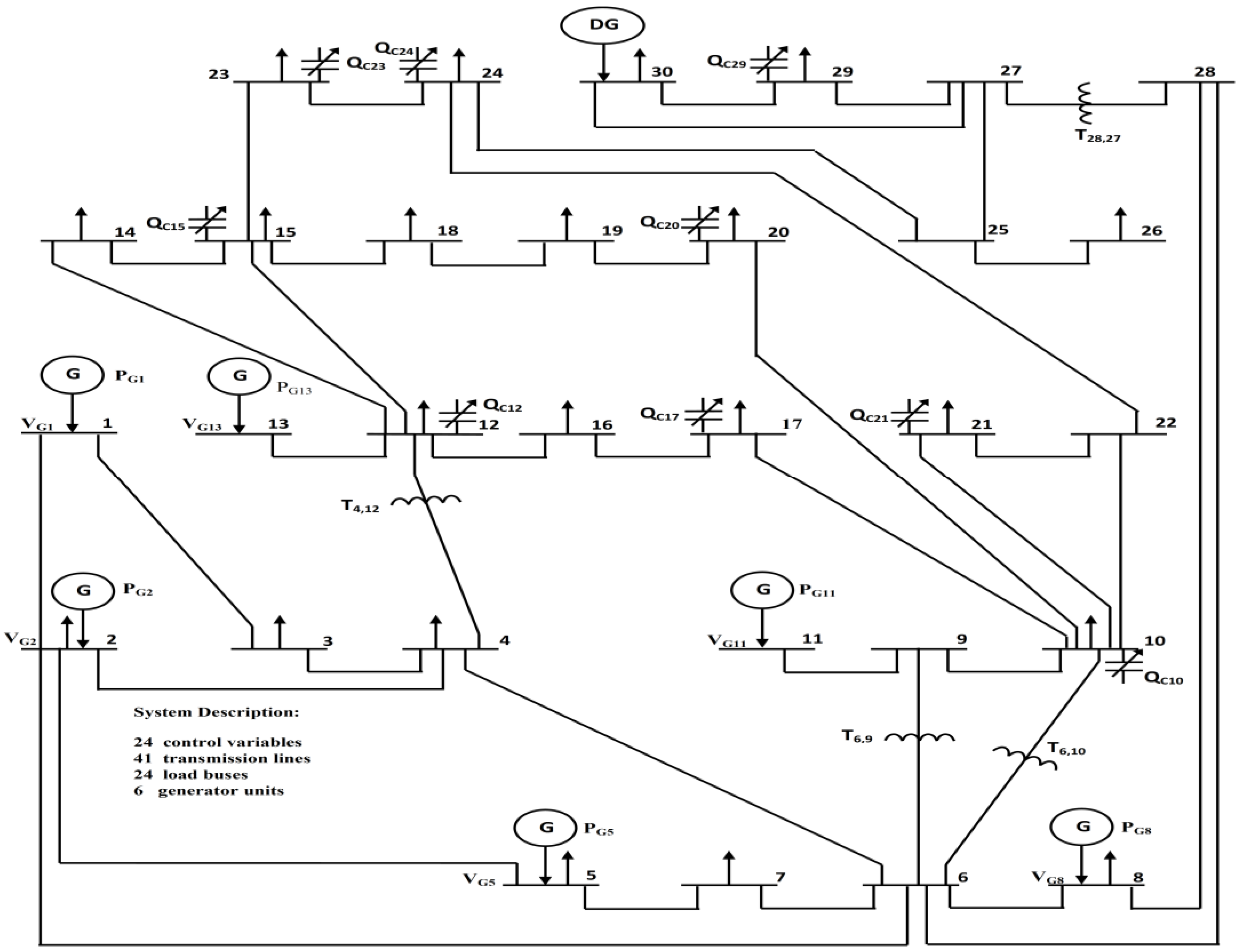
Figure 4.
Convergence graph of fuel cost minimization using the Jaya algorithm with and without employing DG.
Figure 4.
Convergence graph of fuel cost minimization using the Jaya algorithm with and without employing DG.

Figure 5.
Convergence of Jaya method for case 2.

Figure 6.
Convergence of Jaya method for case 3.

Figure 7.
Convergence of Jaya method for case 4.

Table 1.
Optimum setting of control variables for different cases using the Jaya algorithm without and with utilizing DG (modified IEEE 30-bus network).
| Control Variable | Limits | Initial Status | Case 1 | Case 2 | Case 3 | |||||||
|---|---|---|---|---|---|---|---|---|---|---|---|---|
| Min | Max | No DG | DG at bus 30 | DG at bus 3 | No DG | DG at bus 30 | DG at bus 3 | No DG | DG at bus 30 | DG at bus 3 | ||
| PG1 (MW) | 50 | 200 | 99.248 | 177.744 | 169.723 | 169.467 | 51.5093 | 50.2065 | 50.1597 | 154.5292 | 109.7655 | 121.3311 |
| PG2 (MW) | 20 | 80 | 80 | 48.1929 | 47.6388 | 47.9308 | 80 | 79.6863 | 78.3057 | 34.42623 | 64.1610 | 37.9973 |
| PG5 (MW) | 15 | 50 | 50 | 21.4679 | 20.8386 | 21.1194 | 49.9997 | 50 | 48.3094 | 37.20663 | 15 | 43.8276 |
| PG8 (MW) | 10 | 35 | 20 | 21.1103 | 20.6944 | 20.8342 | 35 | 34.4912 | 34.0052 | 17.20772 | 35 | 33.4052 |
| PG11 (MW) | 10 | 30 | 20 | 11.7820 | 11.8375 | 11.8917 | 30 | 29.9970 | 28.9166 | 12.49902 | 15.9857 | 25.8183 |
| PG13 (MW) | 12 | 40 | 20 | 12.1669 | 12.0173 | 12.0307 | 40 | 31.7394 | 38.7597 | 35.41512 | 39.9501 | 16.6108 |
| VG1 (p.u) | 0.95 | 1.1 | 1.05 | 1.08620 | 1.07264 | 1.07033 | 1.06306 | 1.06256 | 1.05922 | 1.05349 | 1.03869 | 1.0509 |
| VG2 (p.u) | 0.95 | 1.1 | 1.04 | 1.06653 | 1.05512 | 1.05308 | 1.05852 | 1.05945 | 1.05699 | 1.03860 | 1.02972 | 1.03385 |
| VG5 (p.u) | 0.95 | 1.1 | 1.01 | 1.03350 | 1.01985 | 1.02076 | 1.03923 | 1.04157 | 1.03384 | 0.99352 | 1.013923 | 1.0494 |
| VG8 (p.u) | 0.95 | 1.1 | 1.01 | 1.03722 | 1.03177 | 1.02941 | 1.04500 | 1.04634 | 1.04006 | 1.04902 | 1.05545 | 1.0266 |
| VG11 (p.u) | 0.95 | 1.1 | 1.05 | 1.09983 | 1.07907 | 1.07827 | 1.09824 | 1.10000 | 1.07218 | 1.09969 | 1.09897 | 1.0694 |
| VG13 (p.u) | 0.95 | 1.1 | 1.05 | 1.05041 | 1.04054 | 1.04283 | 1.05895 | 1.05775 | 1.05832 | 1.09962 | 1.1 | 1.0269 |
| T6,9 | 0.9 | 1.1 | 1.078 | 1.1000 | 1.05793 | 1.06116 | 1.07134 | 1.06605 | 1.0592 | 1.08112 | 1.08192 | 1.0549 |
| T6,10 | 0.9 | 1.1 | 1.069 | 0.90000 | 0.9659 | 0.9782 | 0.93563 | 0.90140 | 0.9677 | 0.90000 | 0.9 | 0.9828 |
| T4,12 | 0.9 | 1.1 | 1.032 | 0.97321 | 1.0021 | 1.0217 | 0.99661 | 1.00208 | 1.0077 | 1.10000 | 1.1 | 1.0068 |
| T28,27 | 0.9 | 1.1 | 1.068 | 0.97869 | 1.0145 | 1.0012 | 0.97796 | 1.01342 | 1.0173 | 0.98312 | 1.01781 | 0.9902 |
| QC10 (Mvar) | 0 | 5 | 0 | 5 | 2.1837 | 2.3639 | 4.95504 | 0 | 4.9107 | 4.99316 | 5 | 2.7804 |
| QC12 (Mvar) | 0 | 5 | 0 | 0.62598 | 2.483 | 2.8944 | 0.05414 | 0 | 3.3384 | 4.97536 | 5 | 2.0184 |
| QC15 (Mvar) | 0 | 5 | 0 | 3.55399 | 1.4851 | 1.7063 | 4.88462 | 4.96356 | 3.8552 | 4.99670 | 5 | 2.2283 |
| QC17 (Mvar) | 0 | 5 | 0 | 4.17065 | 1.6798 | 1.51184 | 4.81859 | 0.17990 | 0.9943 | 5 | 5 | 3.7644 |
| QC20 (Mvar) | 0 | 5 | 0 | 5 | 2.0074 | 2.3638 | 3.55975 | 2.85867 | 1.2218 | 4.73378 | 4.97635 | 2.5031 |
| QC21 (Mvar) | 0 | 5 | 0 | 4.98427 | 1.5623 | 1.7446 | 5 | 5 | 2.2994 | 4.96018 | 5 | 3.0065 |
| QC23 (Mvar) | 0 | 5 | 0 | 3.70495 | 0.9787 | 1.2183 | 3.14258 | 3.90035 | 0.5884 | 5 | 5 | 2.7629 |
| QC24 (Mvar) | 0 | 5 | 0 | 5 | 1.4621 | 1.2115 | 5 | 4.98891 | 1.6599 | 5 | 5 | 2.3394 |
| QC29 (Mvar) | 0 | 5 | 0 | 2.95702 | 1.3188 | 1.1184 | 2.62210 | 0 | 1.1228 | 5 | 0 | 2.9952 |
| Loss (MW) | - | - | 5.8482 | 9.06481 | 8.4983 | 8.9912 | 3.1035 | 2.67504 | 3.3390 | 7.884 | 6.46238 | 5.5903 |
| Cost ($/h) | - | - | 902.0207 | 800.479 | 768.039 | 769.963 | 967.682 | 921.598 | 929.919 | 840.7181 | 816.1612 | 822.2333 |
| Total cost with DG | - | - | - | - | 782.417 | 784.275 | - | 937.746 | 942.489 | - | 832.4112 | 838.4833 |
| Lmax | - | - | 0.1732 | 0.1273 | 0.0969 | 0.1436 | 0.1272 | 0.0892 | 0.1423 | 0.1243 | 0.0851 | 0.1371 |
| QCRM (Mvar) | - | - | 45 | 10.003 | 29.8391 | 28.8669 | 10.963 | 23.1086 | 25.0091 | 0.34082 | 5.02365 | 20.6014 |
| PDG (MW) | 0 | 10 | - | - | 9.1478 | 9.1169 | - | 9.95433 | 8.2827 | - | 10 | 10 |
| QDG (Mvar) | P.F is 0.85 | - | - | 5.6692 | 5.6501 | - | 6.169 | 5.1331 | - | 6.1974 | 6.1974 | |
The values in bold type indicate optimum values.
| Algorithm | Fuel Cost ($/h) | Real Power Losses (MW) | L-Index |
|---|---|---|---|
| Teaching-Learning-Based Optimization (TLBO) [28] | 799.0715 a | 8.626 | 0.1159 |
| DE [14] | 799.2891 a | 8.615 | 0.1226 |
| Lévy Teaching-Learning-Based Optimization (LTLBO) [29] | 799.4369 a | 8.7558 | NA |
| HS [15] | 798.8000 a | 8.6541 | 0.118 |
| GSA [17] | 798.675143 a | 8.386049 | 0.130759 |
| Enhanced Genetic Algorithm (EGA) [12] | 802.06 | NA | NA |
| GPM [26] | 804.853 | 10.486 | NA |
| IGA [11] | 800.805 | NA | NA |
| Enhanced Genetic Algorithm with Decoupled Quadratic Load Flow (EGA-DQLF) [13] | 799.56 a | 8.697 | 0.111 |
| Firefly- Modifed Genetic Algorithm (FFA-mGA) [30] | 801.1128 a | 9.1698 | NA |
| Àdapted Genetic Algorithm with Adjusting Population Size (AGAPOP) [31] | 799.8441 a | 8.9166 | NA |
| BBO [19] | 799.1116 a | 8.63 | NA |
| ABC [4] | 800.66 | 9.0328 | 0.1381 |
| Hybrid Particle Swarm Optimization and Gravitational Search Algorithm (PSOGSA) [23] | 800.49859 | 9.0339 | 0.12674 |
| Jaya | 800.4794 | 9.06481 | 0.1273 |
| Jaya with DG at bus 30 | 768.0398 | 8.5819 | 0.0972 |
The values in bold type indicate optimum values; a Infeasible solution; NA, not available.
| Method | Real Power Loss (MW) | Fuel Cost ($/h) | L-Index |
|---|---|---|---|
| HS [15] | 2.9678 a | 964.5121 | 0.1154 |
| Enhanced Genetic Algorithm with Decoupled Quadratic Load Flow (EGA-DQLF) [13] | 3.2008 | 967.86 | 0.12178 |
| ABC [4] | 3.1078 | 967.681 | 0.1386 |
| Jaya | 3.1035 | 967.6827 | 0.1272 |
| Jaya with DG at bus 30 | 2.675040 | 921.5988 | 0.0892 |
The values in bold type indicate optimum values; a Infeasible solution.
Table 4.
Comparison of the results obtained for voltage stability enhancement (modified IEEE 30-bus network).
| Algorithm | Lmax | Fuel Cost ($/h) | Real Power Losses (MW) |
|---|---|---|---|
| HS [15] | 0.1006 a | 895.6223 | 4.3244 |
| BBO [19] | 0.09803 a | 917.3597 | 4.95 |
| SPEA [32] | 0.1247 a | 898.19 | NA |
| Jaya | 0.1243 | 840.7181 | 7.884 |
| Jaya with DG at bus 30 | 0.0926 | 820.8261 | 5.0110 |
The values in bold type indicate optimum values; a Infeasible solution; NA, not available.
Table 5.
Statistical results obtained over 50 independent trials of Jaya method without and with employing DG.
| Case | No DG | DG (Bus 30) | ||||||
|---|---|---|---|---|---|---|---|---|
| Best | Worst | Average | Standard Deviation | Best | Worst | Average | Standard Deviation | |
| Case 1 | 800.4794 | 800.5306 | 800.4928 | 0.0072 | 768.0398 | 768.0419 | 768.0408 | 0.0084 |
| Case 2 | 3.1035 | 3.1046 | 3.1039 | 0.0038 | 2.675040 | 2.68481 | 2.67925 | 0.0042 |
| Case 3 | 0.1243 | 0.12441 | 0.12432 | 0.00069 | 0.0851 | 0.0856 | 0.0853 | 0.00088 |
Table 6.
Optimum setting of control variables using Jaya algorithm for cost minimization (standard IEEE 118-bus network).
| Control Variable | Case 4 | Control Variable | Case 4 | Control Variable | Case 4 | Control Variable | Case 4 |
|---|---|---|---|---|---|---|---|
| PG1 (MW) | 25.12915 | PG77 (MW) | 0 | VG36 (p.u.) | 1.05974 | VG112 (p.u.) | 1.06284 |
| PG4 (MW) | 0 | PG80 (MW) | 433.1489 | VG40 (p.u.) | 1.05229 | VG113 (p.u.) | 1.05059 |
| PG6 (MW) | 0 | PG85 (MW) | 0 | VG42 (p.u.) | 1.05495 | VG116 (p.u.) | 1.08496 |
| PG8 (MW) | 0 | PG87 (MW) | 3.63259 | VG46 (p.u.) | 1.06267 | T8,5 | 1.0173 |
| PG10 (MW) | 402.65452 | PG89 (MW) | 505.2258 | VG49 (p.u.) | 1.07502 | T26,25 | 1.07480 |
| PG12 (MW) | 85.61712 | PG90 (MW) | 0 | VG54 (p.u.) | 1.05626 | T30,17 | 1.05160 |
| PG15 (MW) | 18.98469 | PG91 (MW) | 0 | VG55 (p.u.) | 1.05611 | T38,37 | 0.98400 |
| PG18 (MW) | 11.47358 | PG92 (MW) | 0 | VG56 (p.u.) | 1.05592 | T63,59 | 1.03480 |
| PG19 (MW) | 20.16029 | PG99 (MW) | 0 | VG59 (p.u.) | 1.07109 | T64,61 | 0.9752 |
| PG24 (MW) | 0 | PG100 (MW) | 231.9774 | VG61 (p.u.) | 1.07961 | T65,66 | 0.9721 |
| PG25 (MW) | 195.35572 | PG103 (MW) | 38.30151 | VG62 (p.u.) | 1.07462 | T68,69 | 0.9629 |
| PG26 (MW) | 281.99696 | PG104 (MW) | 0 | VG65 (p.u.) | 1.08247 | T81,80 | 1.0047 |
| PG27 (MW) | 11.53285 | PG105 (MW) | 4.55102 | VG66 (p.u.) | 1.087499 | QC34 (Mvar) | 17.2517 |
| PG31 (MW) | 7.2456650 | PG107 (MW) | 28.03098 | VG69 (p.u.) | 1.09579 | QC44 (Mvar) | 5.0382 |
| PG32 (MW) | 15.691750 | PG110 (MW) | 6.86202 | VG70 (p.u.) | 1.07252 | QC45 (Mvar) | 22.7408 |
| PG34 (MW) | 0.97016 | PG111 (MW) | 35.28710 | VG72 (p.u.) | 1.06673 | QC46 (Mvar) | 2.5184 |
| PG36 (MW) | 7.10474 | PG112 (MW) | 35.55218 | VG73 (p.u.) | 1.07050 | QC48 (Mvar) | 6.2933 |
| PG40 (MW) | 47.03167 | PG113 (MW) | 0 | VG74 (p.u.) | 1.05715 | QC74 (Mvar) | 11.7396 |
| PG42 (MW) | 39.88786 | PG116 (MW) | 0 | VG76 (p.u.) | 1.04725 | QC79 (Mvar) | 26.2949 |
| PG46 (MW) | 19.03365 | VG1 (p.u.) | 1.03506 | VG77 (p.u.) | 1.08098 | QC82 (Mvar) | 27.4917 |
| PG49 (MW) | 193.84281 | VG4 (p.u.) | 1.06279 | VG80 (p.u.) | 1.09254 | QC83 (Mvar) | 7.29930 |
| PG54 (MW) | 49.47427 | VG6 (p.u.) | 1.05461 | VG85 (p.u.) | 1.08276 | QC105 (Mvar) | 19.6392 |
| PG55 (MW) | 30.83240 | VG8 (p.u.) | 1.08258 | VG87 (p.u.) | 1.08774 | QC107 (Mvar) | 4.8172 |
| PG56 (MW) | 31.18303 | VG10 (p.u.) | 1.08589 | VG89 (p.u.) | 1.08959 | QC110 (Mvar) | 23.9717 |
| PG59 (MW) | 149.75472 | VG12 (p.u.) | 1.05108 | VG90 (p.u.) | 1.07176 | Loss (MW) | 74.519 |
| PG61 (MW) | 148.79525 | VG15 (p.u.) | 1.04536 | VG91 (p.u.) | 1.07561 | Cost ($/h) | 129,490.54 |
| PG62 (MW) | 0 | VG18 (p.u.) | 1.04583 | VG92 (p.u.) | 1.08039 | QCRM (Mvar) | 184.904 |
| PG65 (MW) | 354.25856 | VG19 (p.u.) | 1.04575 | VG99 (p.u.) | 1.08412 | - | - |
| PG66 (MW) | 351.00337 | VG24 (p.u.) | 1.06729 | VG100 (p.u.) | 1.08739 | - | - |
| PG69 (MW) | 457.25440 | VG25 (p.u.) | 1.07470 | VG103 (p.u.) | 1.08028 | - | - |
| PG70 (MW) | 0 | VG26 (p.u.) | 1.09339 | VG104 (p.u.) | 1.07172 | - | - |
| PG72 (MW) | 0 | VG27 (p.u.) | 1.05391 | VG105 (p.u.) | 1.06932 | - | - |
| PG73 (MW) | 0 | VG31 (p.u.) | 1.04382 | VG107 (p.u.) | 1.06308 | - | - |
| PG74 (MW) | 16.10096 | VG32 (p.u.) | 1.05110 | VG110 (p.u.) | 1.07020 | - | - |
| PG76 (MW) | 21.57844 | VG34 (p.u.) | 1.06450 | VG111 (p.u.) | 1.077691 | - | - |
Bold type indicates optimum value.
| Algorithm | Fuel Cost ($/h) | Real Power Losses (MW) |
|---|---|---|
| Teaching-Learning-Based Optimization (TLBO) [28] | 129,682.844 | NA |
| Gravitational Search Algorithm (GSA) [34] | 129,565 | 76.19 |
| Biogeography-Based Optimisation (BBO) [34] | 129,686 | 78.14 |
| Particle Swarm Optimization(PSO) [35] | 130,288.21 | NA |
| Differential Evolution (DE) [36] | 129,582 | 79.41 |
| Grey Wolf Optimizer (GWO) [36] | 129,720 | 79.58 |
The values in bold type indicate optimum values; NA, not available.
© 2016 by the authors; licensee MDPI, Basel, Switzerland. This article is an open access article distributed under the terms and conditions of the Creative Commons Attribution (CC-BY) license (http://creativecommons.org/licenses/by/4.0/).
Share and Cite
MDPI and ACS Style
Warid, W.; Hizam, H.; Mariun, N.; Abdul-Wahab, N.I. Optimal Power Flow Using the Jaya Algorithm. Energies 2016, 9, 678. https://doi.org/10.3390/en9090678
AMA Style
Warid W, Hizam H, Mariun N, Abdul-Wahab NI. Optimal Power Flow Using the Jaya Algorithm. Energies. 2016; 9(9):678. https://doi.org/10.3390/en9090678
Chicago/Turabian StyleWarid, Warid, Hashim Hizam, Norman Mariun, and Noor Izzri Abdul-Wahab. 2016. "Optimal Power Flow Using the Jaya Algorithm" Energies 9, no. 9: 678. https://doi.org/10.3390/en9090678
Note that from the first issue of 2016, this journal uses article numbers instead of page numbers. See further details here.