
State-of-Charge Estimation for Lithium-Ion Batteries Using a Kalman Filter Based on Local Linearization

Abstract
:1. Introduction
2. System Modeling
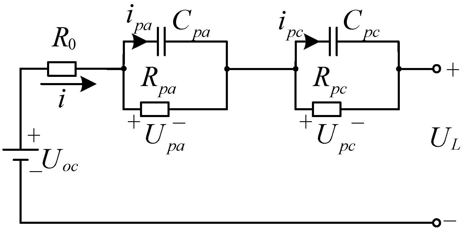
2.1. Equivalent Circuit Model

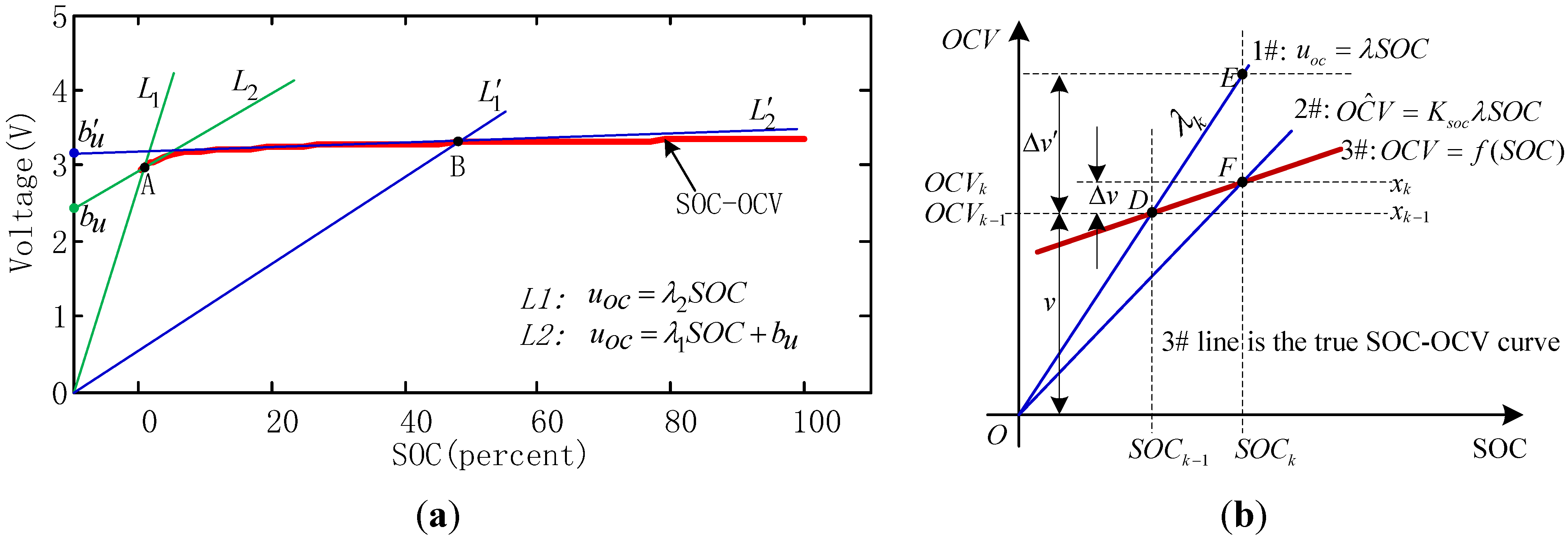
2.2. Linearization
2.2.1. Method

2.2.2. Linearization Parameters Identification
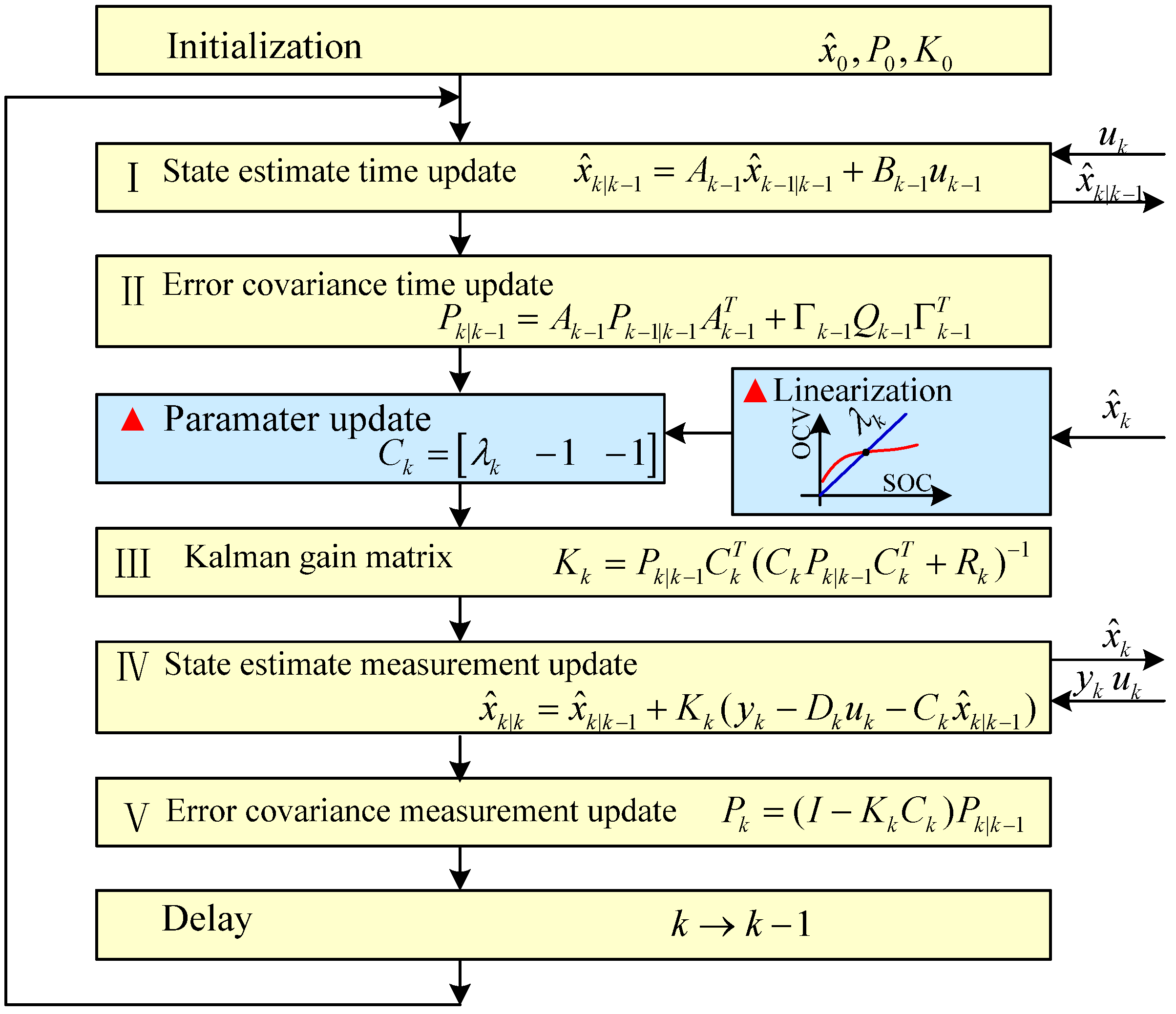
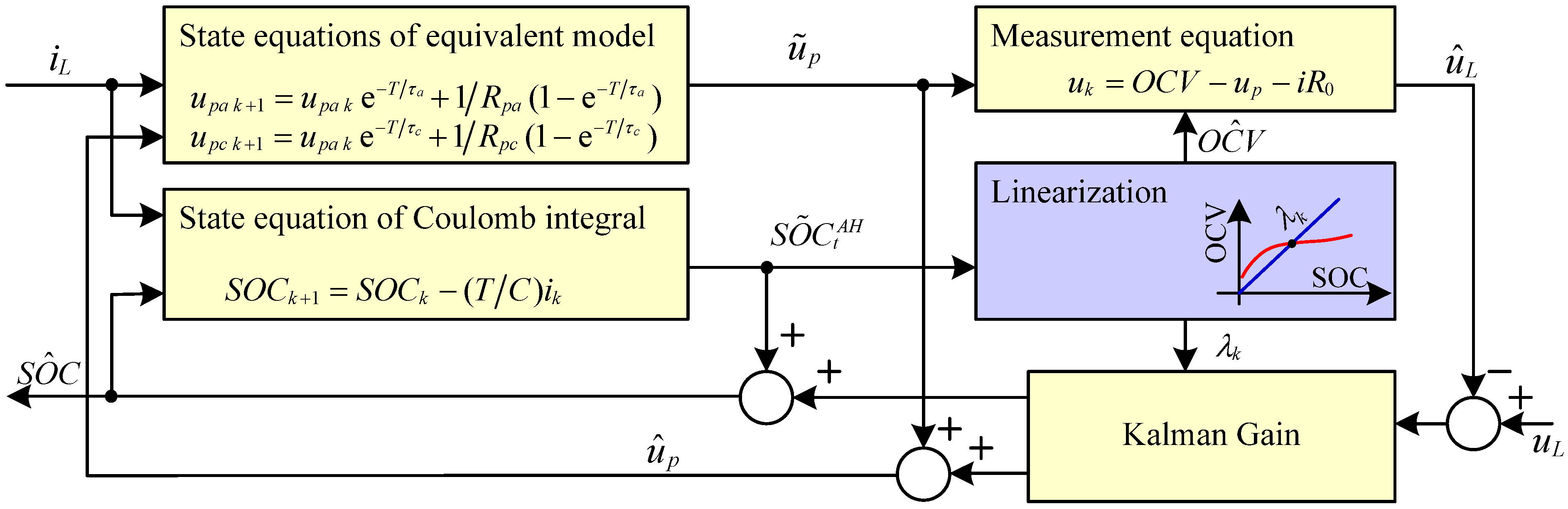
2.3. Kalman Filter Based on the Equivalent Circuit Model
2.4. Mechanism of Linearization
3. Experiments and Results


| Component of | Values |
|---|---|
| K0 | 3149.30 − 105.00i |
| K1 | 288.24 − 105.77i |
| K2 | 0.5748 + 0.0408i |
| K3 | 54.8063 − 57.1211i |
| K4 | 29.8337 + 60.3188i |
| Cost function | Goodness of Fit |
|---|---|
| Mean square error | 171.0662 |
| Normalized root mean square error | 0.8666 |
| Normalized mean square error | 0.9822 |
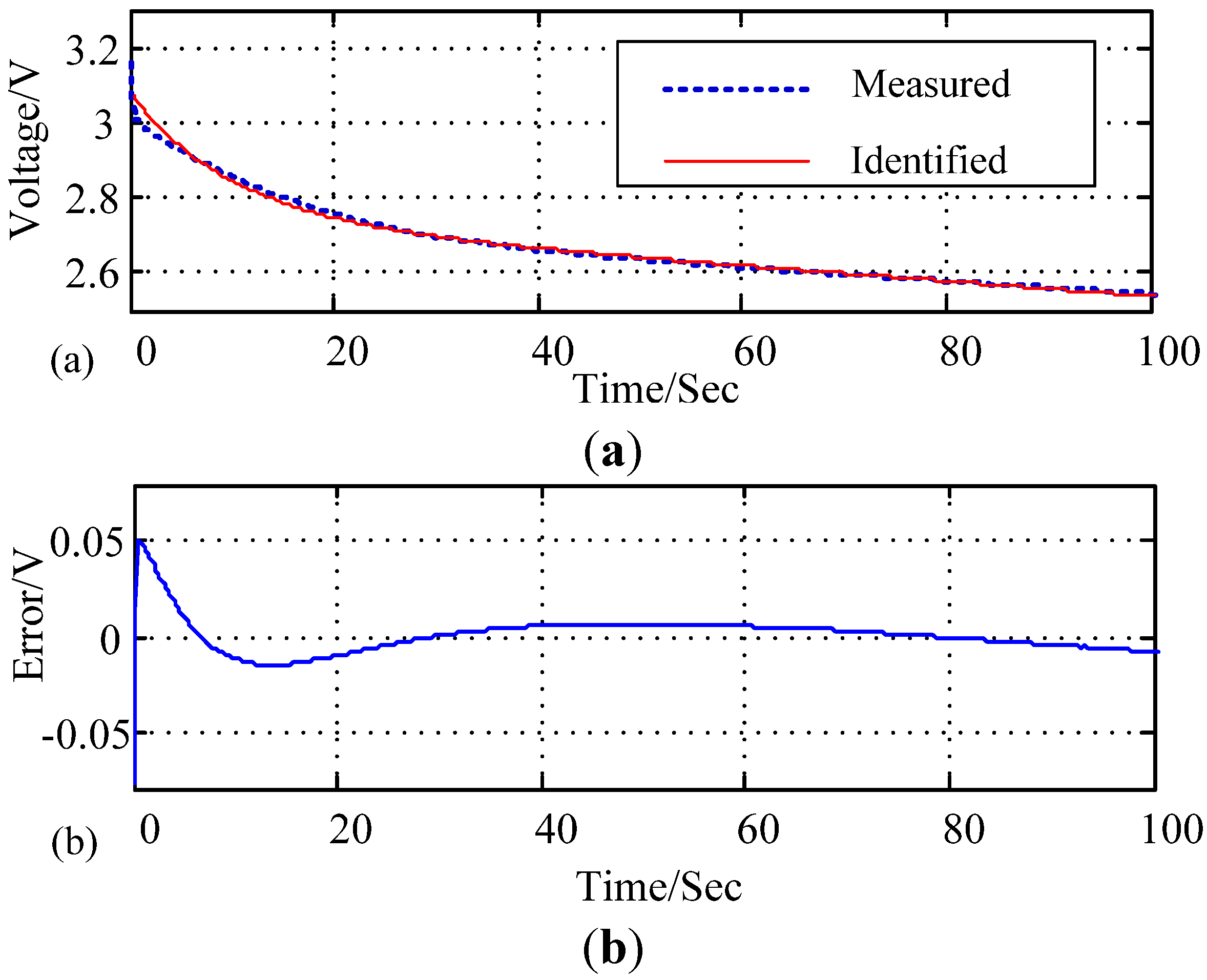
3.1. Parameter Identification
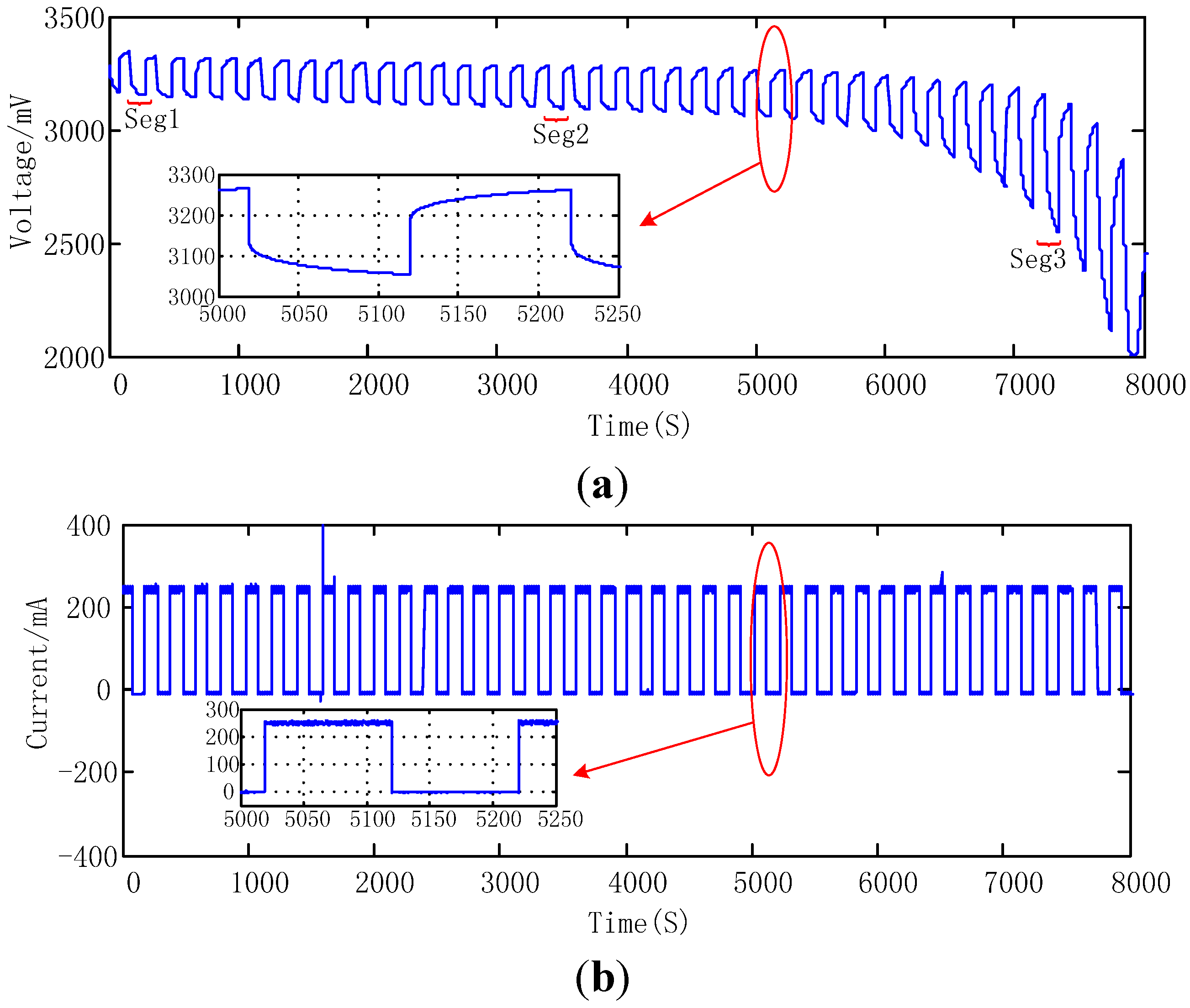

| Parameter | Seg1 | Seg2 | Seg3 |
|---|---|---|---|
| Time/Sec | 201–302 | 3429.700–3530.500 | 7262.300–7363.100 |
| /Ω | 0.017833 | 0.077258 | 0.900000 |
| /Ω | 0.566761 | 0.579680 | 1.384719 |
| /F | 0.176441 | 0.334183 | 7.221680 |
| /Sec | 0.1000 | 0.1937 | 10.0000 |
| /Ω | 0.233619 | 0.196233 | 4530.766481 |
| /F | 127.351684 | 160.522833 | 118.879036 |
| /Sec | 29.7518 | 31.4998 | 538613.1511 |
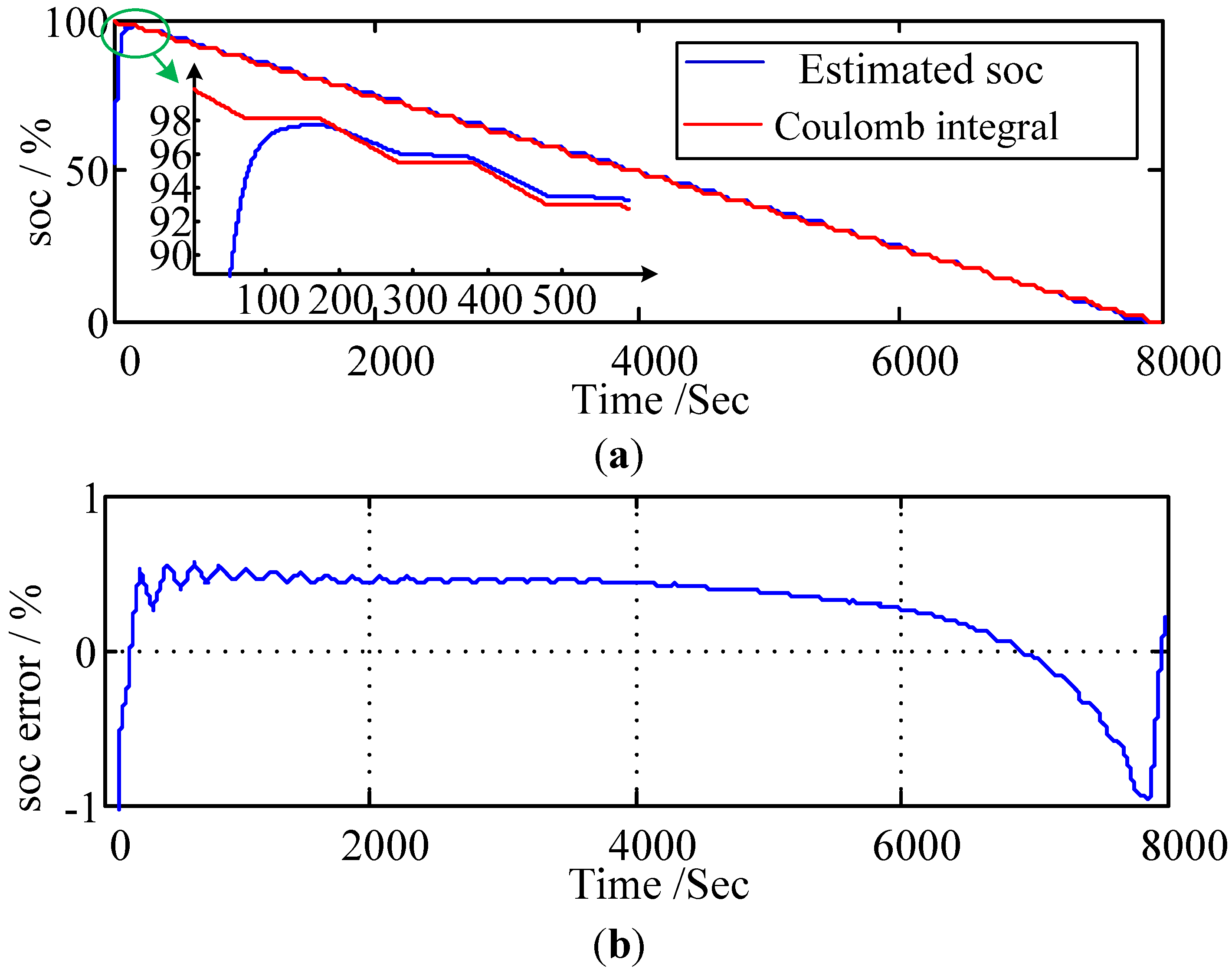
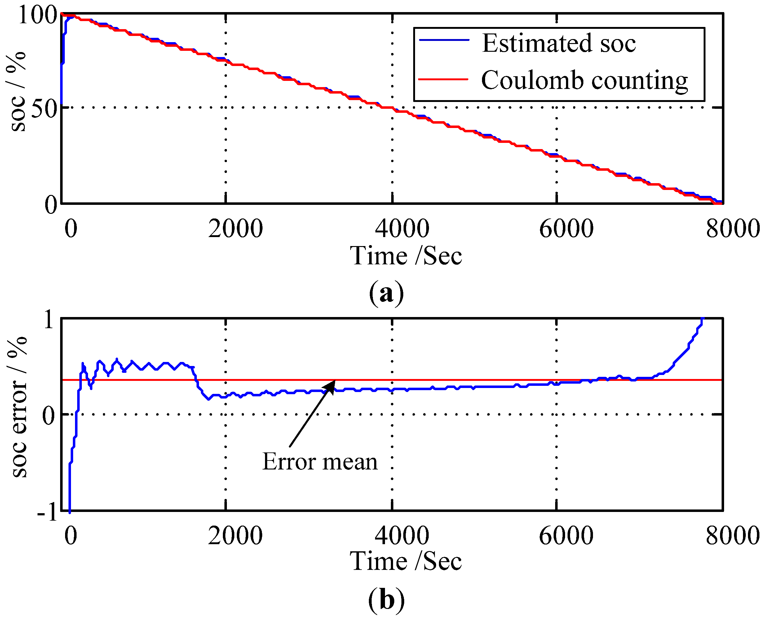
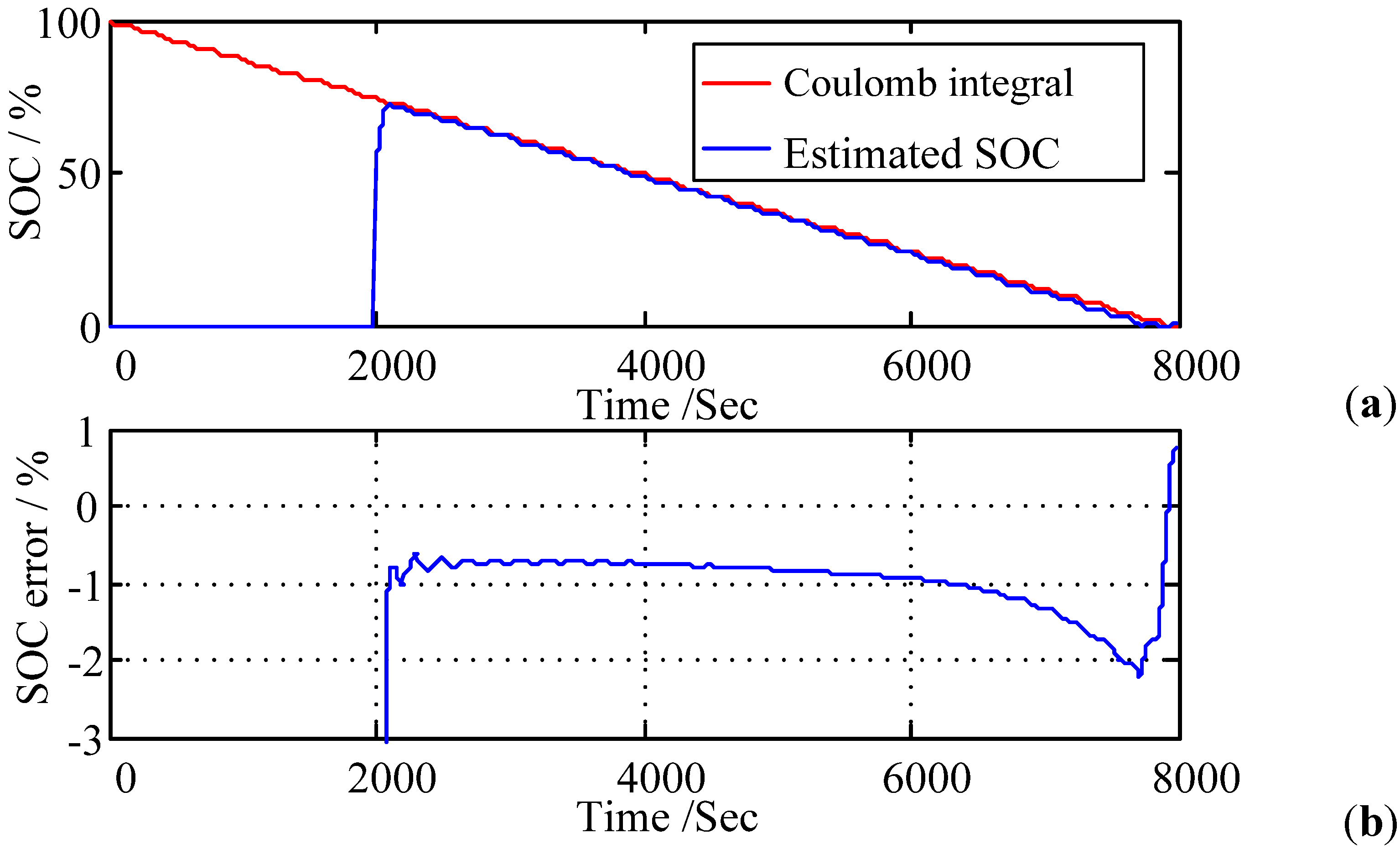
3.2. SOC Estimation
| Variable | Unit | Explanation | Value |
|---|---|---|---|
| SOC0 | V | State of charge | 0.5 |
| Upa0 | V | Fast transient voltage | 0.01 |
| Upc0 | V | Slow transient voltage | 0.05 |
| Q | - | System noise covariance | 0.000001 |
| R | - | Measurement noise covariance | 22 |


3.3. Error Influence


3.4. SOC Estimation for a Partly Charged Battery
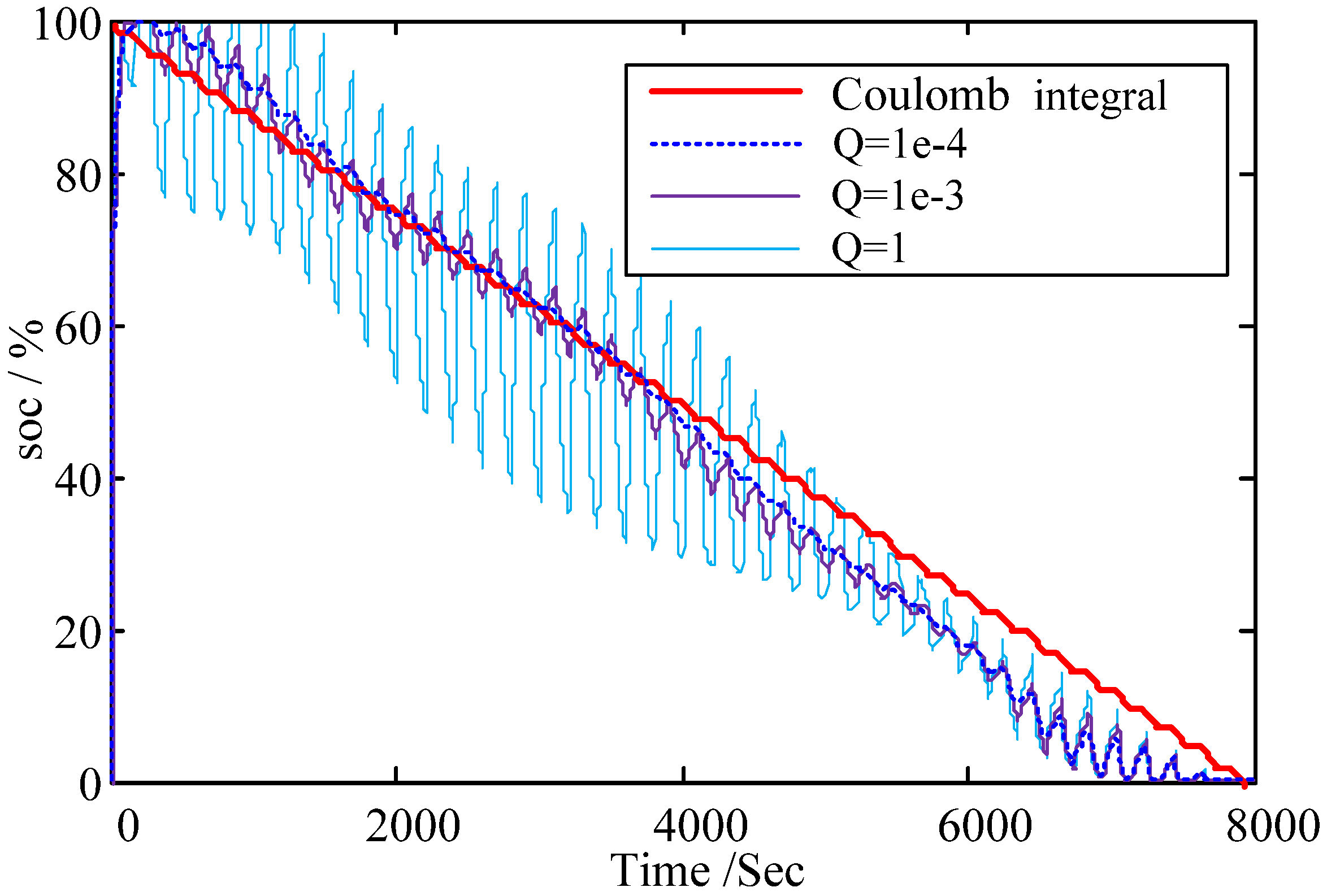
3.5. System Error and Noise

4. Discussion
4.1. Principle of Linearization
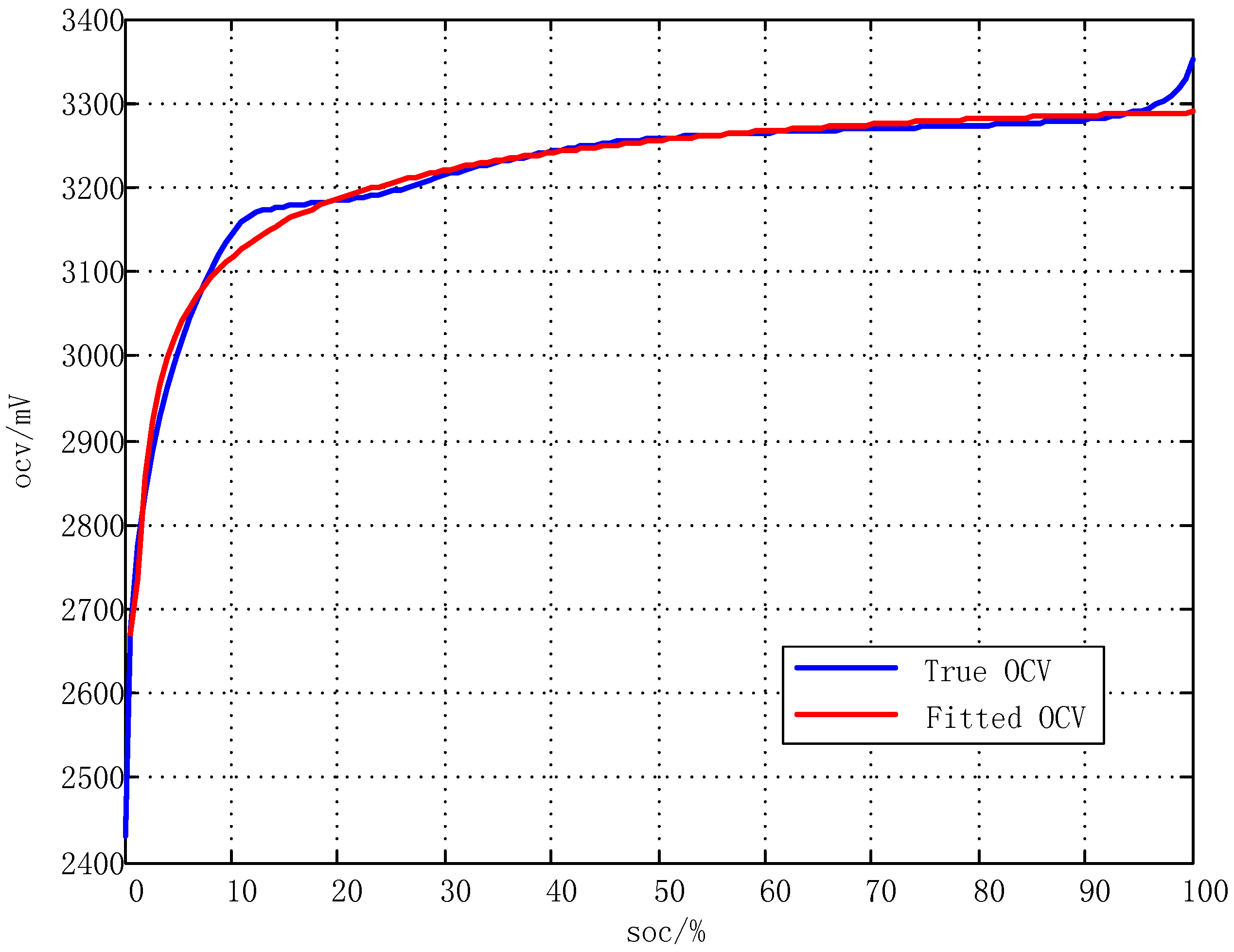
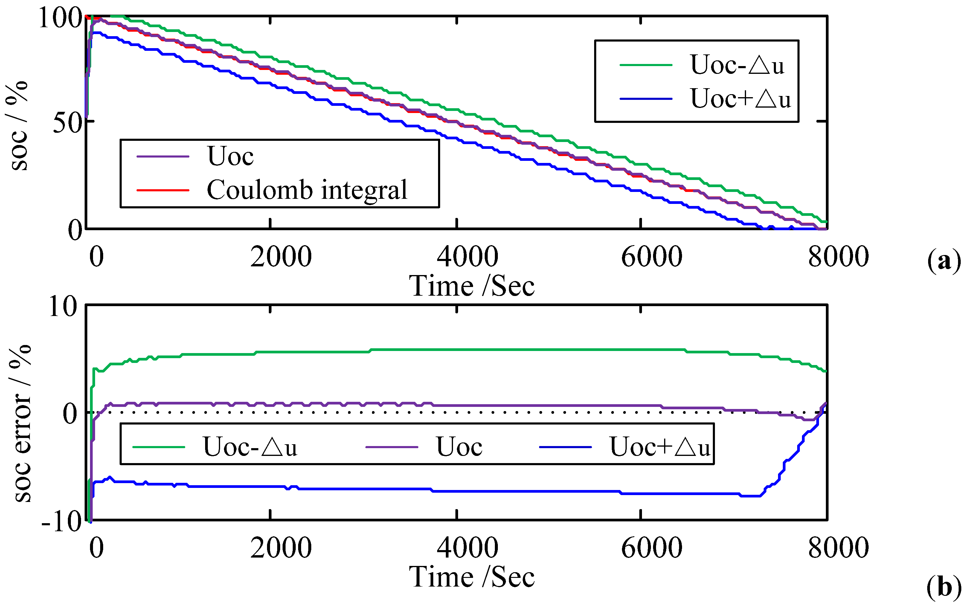
4.2. Influence of OCV Estimation

5. Conclusions
Acknowledgments
Author Contributions
Conflicts of Interest
References
- Khan, M.R.; Mulder, G.; Van Mierlo, J. An online framework for state of charge determination of battery systems using combined system identification approach. J. Power Sources 2014, 246, 629–641. [Google Scholar] [CrossRef]
- Gholizadeh, M.; Salmasi, F.R. Estimation of state of charge, unknown nonlinearities, and state of health of a lithium-ion battery based on a comprehensive unobservable model. IEEE Trans. Ind. Electron. 2014, 61, 1335–1344. [Google Scholar] [CrossRef]
- Truchot, C.; Dubarry, M.; Liaw, B.Y. State-of-charge estimation and uncertainty for lithium-ion battery strings. Appl. Energy 2014, 119, 218–227. [Google Scholar] [CrossRef]
- Liu, L.; Wang, L.Y.; Chen, Z.; Wang, C.; Lin, F.; Wang, H. Integrated system identification and state-of-charge estimation of battery systems. IEEE Trans. Energy Convers. 2013, 28, 12–23. [Google Scholar] [CrossRef]
- Xing, Y.; He, W.; Pecht, M.; Tsui, K.L. State of charge estimation of lithium-ion batteries using the open-circuit voltage at various ambient temperatures. Appl. Energy 2014, 113, 106–115. [Google Scholar] [CrossRef]
- Omar, N.; Monem, M.A.; Firouz, Y.; Salminen, J.; Smekens, J.; Hegazy, O.; Gaulous, H.; Mulder, G.; Van den Bossche, P.; Coosemans, T.; et al. Lithium iron phosphate based battery—Assessment of the aging parameters and development of cycle life model. Appl. Energy 2014, 113, 1575–1585. [Google Scholar] [CrossRef]
- Sepasi, S.; Ghorbani, R.; Liaw, B.Y. Improved extended kalman filter for state of charge estimation of battery pack. J. Power Sources 2014, 255, 368–376. [Google Scholar] [CrossRef]
- Mastali, M.; Vazquez-Arenas, J.; Fraser, R.; Fowler, M.; Afshar, S.; Stevens, M. Battery state of the charge estimation using kalman filtering. J. Power Sources 2013, 239, 294–307. [Google Scholar] [CrossRef]
- Yuan, S.; Wu, H.; Yin, C. State of charge estimation using the extended kalman filter for battery management systems based on the arx battery model. Energies 2013, 6, 444–470. [Google Scholar] [CrossRef]
- Zhang, C.; Jiang, J.; Zhang, W.; Sharkh, S.M. Estimation of state of charge of lithium-ion batteries used in HEV using robust extended Kalman filtering. Energies 2012, 5, 1098–1115. [Google Scholar] [CrossRef]
- Andre, D.; Appel, C.; Soczka-Guth, T.; Sauer, D.U. Advanced mathematical methods of SOC and SOH estimation for lithium-ion batteries. J. Power Sources 2013, 224, 20–27. [Google Scholar] [CrossRef]
- He, W.; Williard, N.; Chen, C.; Pecht, M. State of charge estimation for electric vehicle batteries using unscented kalman filtering. Microelectron. Reliab. 2013, 53, 840–847. [Google Scholar] [CrossRef]
- Xia, B.; Chen, C.; Tian, Y.; Sun, W.; Xu, Z.; Zheng, W. A novel method for state of charge estimation of lithium-ion batteries using a nonlinear observer. J. Power Sources 2014, 270, 359–366. [Google Scholar] [CrossRef]
- Rahimi-Eichi, H.; Baronti, F.; Chow, M.-Y. Online adaptive parameter identification and state-of-charge coestimation for lithium-polymer battery cells. IEEE Trans. Ind. Electron. 2014, 61, 2053–2061. [Google Scholar] [CrossRef]
- Hametner, C.; Jakubek, S. State of charge estimation for lithium ion cells: Design of experiments, nonlinear identification and fuzzy observer design. J. Power Sources 2013, 238, 413–421. [Google Scholar] [CrossRef]
- Sepasi, S.; Ghorbani, R.; Liaw, B.Y. A novel on-board state-of-charge estimation method for aged Li-ion batteries based on model adaptive extended kalman filter. J. Power Sources 2014, 245, 337–344. [Google Scholar] [CrossRef]
- Moura, S.J.; Chaturvedi, N.A.; Krstic, M. Adaptive partial differential equation observer for battery state-of-charge/state-of-health estimation via an electrochemical model. J. Dyn. Syst. Meas. Contr. Trans. ASME 2014, 136, 011015. [Google Scholar] [CrossRef]
- Shahriari, M.; Farrokhi, M. Online state-of-health estimation of vrla batteries using state of charge. IEEE Trans. Ind. Electron. 2013, 60, 191–202. [Google Scholar] [CrossRef]
- Xiong, R.; Sun, F.; Gong, X.; Gao, C. A data-driven based adaptive state of charge estimator of lithium-ion polymer battery used in electric vehicles. Appl. Energy 2014, 113, 1421–1433. [Google Scholar] [CrossRef]
- Fleischer, C.; Waag, W.; Heyn, H.-M.; Sauer, D.U. On-line adaptive battery impedance parameter and state estimation considering physical principles in reduced order equivalent circuit battery models part 2. Parameter and state estimation. J. Power Sources 2014, 262, 457–482. [Google Scholar] [CrossRef]
- Chen, M.; Rincon-Mora, G.A. Accurate electrical battery model capable of predicting runtime and I-V performance. IEEE Trans. Energy Convers. 2006, 21, 504–511. [Google Scholar] [CrossRef]
- He, H.; Xiong, R.; Fan, J. Evaluation of lithium-ion battery equivalent circuit models for state of charge estimation by an experimental approach. Energies 2011, 4, 582–598. [Google Scholar] [CrossRef]
- Sun, F.; Xiong, R.; He, H. Estimation of state-of-charge and state-of-power capability of lithium-ion battery considering varying health conditions. J. Power Sources 2014, 259, 166–176. [Google Scholar] [CrossRef]
- Weng, C.; Cui, Y.; Sun, J.; Peng, H. On-board state of health monitoring of lithium-ion batteries using incremental capacity analysis with support vector regression. J. Power Sources 2013, 235, 36–44. [Google Scholar] [CrossRef]
- Chen, Z.; Fu, Y.; Mi, C.C. State of charge estimation of lithium-ion batteries in electric drive vehicles using extended Kalman filtering. IEEE Trans. Veh. Technol. 2013, 62, 1020–1030. [Google Scholar] [CrossRef]
- Plett, G.L. Extended Kalman filtering for battery management systems of Lipb-based HEV battery packs—Part 2. Modeling and identification. J. Power Sources 2004, 134, 262–276. [Google Scholar] [CrossRef]
© 2015 by the authors; licensee MDPI, Basel, Switzerland. This article is an open access article distributed under the terms and conditions of the Creative Commons Attribution license (http://creativecommons.org/licenses/by/4.0/).
Share and Cite
Yu, Z.; Huai, R.; Xiao, L. State-of-Charge Estimation for Lithium-Ion Batteries Using a Kalman Filter Based on Local Linearization. Energies 2015, 8, 7854-7873. https://doi.org/10.3390/en8087854
Yu Z, Huai R, Xiao L. State-of-Charge Estimation for Lithium-Ion Batteries Using a Kalman Filter Based on Local Linearization. Energies. 2015; 8(8):7854-7873. https://doi.org/10.3390/en8087854
Chicago/Turabian StyleYu, Zhihao, Ruituo Huai, and Linjing Xiao. 2015. "State-of-Charge Estimation for Lithium-Ion Batteries Using a Kalman Filter Based on Local Linearization" Energies 8, no. 8: 7854-7873. https://doi.org/10.3390/en8087854
APA StyleYu, Z., Huai, R., & Xiao, L. (2015). State-of-Charge Estimation for Lithium-Ion Batteries Using a Kalman Filter Based on Local Linearization. Energies, 8(8), 7854-7873. https://doi.org/10.3390/en8087854