Article

Wind Power Grid Connected Capacity Prediction Using LSSVM Optimized by the Bat Algorithm

Department of Economics and Management, North China Electric Power University, Baoding 071003, China
*
Author to whom correspondence should be addressed.
Energies 2015, 8(12), 14346-14360; https://doi.org/10.3390/en81212428
Submission received: 21 November 2015 / Revised: 14 December 2015 / Accepted: 15 December 2015 / Published: 18 December 2015

Abstract

:
Given the stochastic nature of wind, wind power grid-connected capacity prediction plays an essential role in coping with the challenge of balancing supply and demand. Accurate forecasting methods make enormous contribution to mapping wind power strategy, power dispatching and sustainable development of wind power industry. This study proposes a bat algorithm (BA)–least squares support vector machine (LSSVM) hybrid model to improve prediction performance. In order to select input of LSSVM effectively, Stationarity, Cointegration and Granger causality tests are conducted to examine the influence of installed capacity with different lags, and partial autocorrelation analysis is employed to investigate the inner relationship of grid-connected capacity. The parameters in LSSVM are optimized by BA to validate the learning ability and generalization of LSSVM. Multiple model sufficiency evaluation methods are utilized. The research results reveal that the accuracy improvement of the present approach can reach about 20% compared to other single or hybrid models.

1. Literature Review

As one of the most proven forms of environmentally friendly and renewable energy, wind power continues to attract considerable attention throughout the world [1,2,3,4]. In 2014, the new installed capacity of global wind power was 51,477 MW, of which China accounted for 45.4%, explicitly becoming a global leader pertaining to wind power capacity. However, this rapid integration of wind power into the grid has resulted in many operational challenges in the distribution networks since most wind farms are directly connected to the distribution network instead of the transmission network. The benefit of rapid extension of the distribution system is incident to the operational challenges. Although they have started to create impact on the overall power system operation, until recently no support were imperatively offered to the distribution/transmission system operation [5]. For instance, the overwhelming scale and speed of deployment are now embarrassing China’s wind power industry due to grid connectivity issues. The problem of “abandoned wind” in China has led to more than 100 billion kWh of power being wasted. The disconnection between the rapid increase of wind power supply and grid-connected consumption hinders the sustainable development of the wind power industry. As the literature on grid-connected capacity prediction only gives scant regard to the disorderly expansion of wind power, there appeared to be a situation of repeated construction and “surplus production”. Therefore, the precise forecasting approaches with respect to grid-connected capacity have positive implications on the reduction of the wasted energy and the healthy and stable development of the wind power industry.
There is abundant literature on wind power predication, most of which has been published during the past few years. The predication literature covers many aspects of wind power. These include, but are not limited to, wind speed forecasting, generated power and generated energy prediction, relatively with little attention to wind power grid connected capacity prediction. The methods of these studies can be classified into two categories: time series models and artificial intelligent algorithm models. Most of these approaches utilize time series analysis, encompassing vector autoregressive (VAR) models [6,7] and autoregressive moving average (AMRA) models [7,8,9,10]. Torres [8] decribed a modified ARMA model owing to the non-Gaussian nature and the non-stationary nature of wind, and the method behaved especially well in longer-term forecasting. Erdem [9] decomposed wind speed into lateral and longitudinal components with each component being represented by an ARMA model, then the results were combined to obtain predictive values. Liu [10] proposed an ARMA–GARCH algorithm for modeling the mean and volatility of wind speed, with the model being evaluated the effectiveness through multiple methods. The results suggested the current approach effectively grasped the trend of wind speed. Jiang [11] presented a hybrid model of autoregressive moving average and generalized autoregressive conditional heteroscedasticity to forecast wind speed. The simulation results demonstrated the proposed method outperformed the compared approaches. Nevertheless, the extensive implementation of time series model on wind power prediction can be problematic, since it has poor nonlinear fitting performance.
Conversely, the adaptive and self-organized learning characteristics of intelligent algorithms apparently validate the estimation of nonlinear time series. For instance, artificial neural network (ANN) [12,13,14,15,16,17] and LSSVM [17,18,19,20] are perceived to be highly effective methods in the field of wind power forecasting. Guo [18] successfully conducted a hybrid Seasonal Auto-Regression Integrated Moving Average and Least Square Support Vector Machine (SARIMA-LSSVM) model to predict the mean monthly wind speed. De Giorgi [19] developed a comparative study for the prediction of the power production of a wind farm, using historical data and numerical weather predictions. It was illustrated that the hybrid approach based on WD-LSSVM significantly outperformed hybrid artificial neural network (ANN)-based methods. Yuan [20] established a LSSVM model with the light of gravitational search algorithm (GSA) for short-term output power prediction of a wind farm. Compared with the back propagation (BP) neural network and support vector machine (SVM) model, the modeling results indicated that the GSA–LSSVM model had higher accuracy for short-term output power prediction. Wang [21] decomposed the non-stationary time series into several intrinsic mode functions (IMF) and the trend item, then each IMF was forecasted by diverse LSSVM models. These forecasting results of each IMF were combined to gain the final value of output power of the wind farm.
With the rapid development of artificial intelligence technology, many scholars are devoting growing time and resources to delve deeper into LSSVM. Since the regularization parameter c and the kernel parameter σ of the LSSVM have a great influence on the performance of the prediction model, a body of studies established LSSVM model based on different intelligent algorithms for wind power prediction achieving better overall results [21,22,23,24]. Hu [22] constructed a corrected quantum particle swarm optimization (QPSO) algorithm for LSSVM parameters selection, and as a result, the generalization capability and learning performance of LSSVM model was clearly enhanced. Sun [23] introduced a LSSVM model optimized by PSO. The simulation results recognized that the proposed method can distinctly increase the predicting accuracy. Wang [24] designed a LSSVM model, the parameters of which were tuned by a particle swarm optimization based on simulated annealing (PSOSA). Four wind farms as a case study in Gansu Province, Northwest China were applied to corroborate the effectiveness of the hybrid model. Song [25] employed a novel hybrid prediction model using harmony search (HS) and LSSVM. In the pilot study, HS addressed the issue of the blindness of parameter selection and kernel function of LSSVM, realizing the adaptive selections of regularization parameter c and kernel function parameter σ. Compared with the BP neural network and traditional statistical regression model, the HS–LSSVM model had higher precision and forecasting efficiency.
However, it is clear that from the previous research that PSO results in a local optimum during the regularization parameter selection process. In addition the weak local search ability of the HS algorithm has negative implications on the convergence rate. In order to implement the shortcomings of existing algorithms, in 2010, a new global algorithm, namely, the bat algorithm (BA), was developed by Yang, based on the echolocation behavior of bats [26]. With a good combination of the paramount advantages of PSO, genetic algorithm (GA) and HS, the superiority of BA relies on its simplification, powerful searching ability and fast convergence. Recently, a burgeoning number of studies are focusing on BA for parameter optimization [26,27,28,29,30]. Hafezi [27] exploited a compound BA strategy to predict stock prices over a long term period. The model was tested for forecasting eight years of DAX stock prices in quarterly periods and was perceived as a suitable tool for predicting stock prices. Meng [28] applied a novel bat algorithm (NBA) to four real-world engineering designs, and the effectiveness, efficiency and stability of NBA in the light of biological basis were noticeably promoted. Senthilkumar [29] selected the best set of features from the initial sets through BA conceived as one of the recent optimization algorithm for reducing the time consumption in detecting record duplication. Venkateswara Rao [30] adopted BA to minimize real power losses in a power system for generation reallocation with unified power flow controller. Yang [31] explored a new multi-objective optimization approach on the basis of BA to suppress critical harmonics and foster power factor for passive power filters (PPFs). Considering the excellent performance of BA in the process of parameter optimization, it is the purpose of the present paper to utilize BA to select the two pertinent parameters of the LSSVM model and gain the global optimal solution.
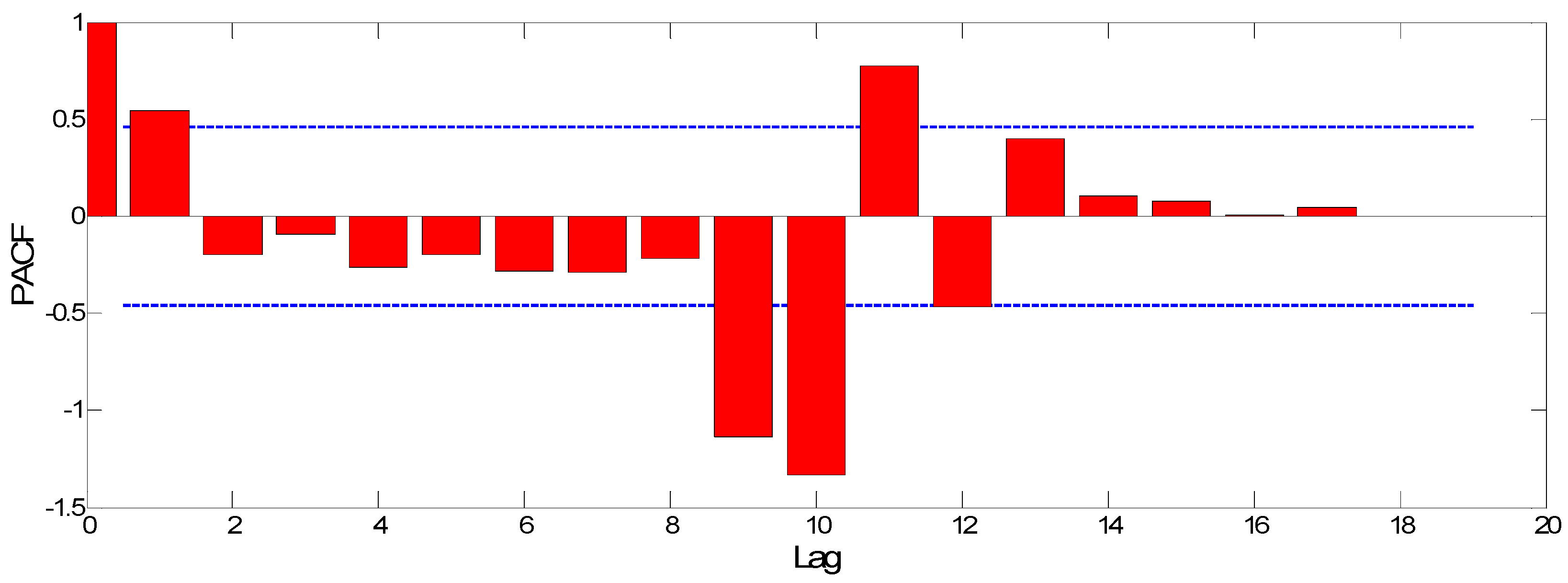
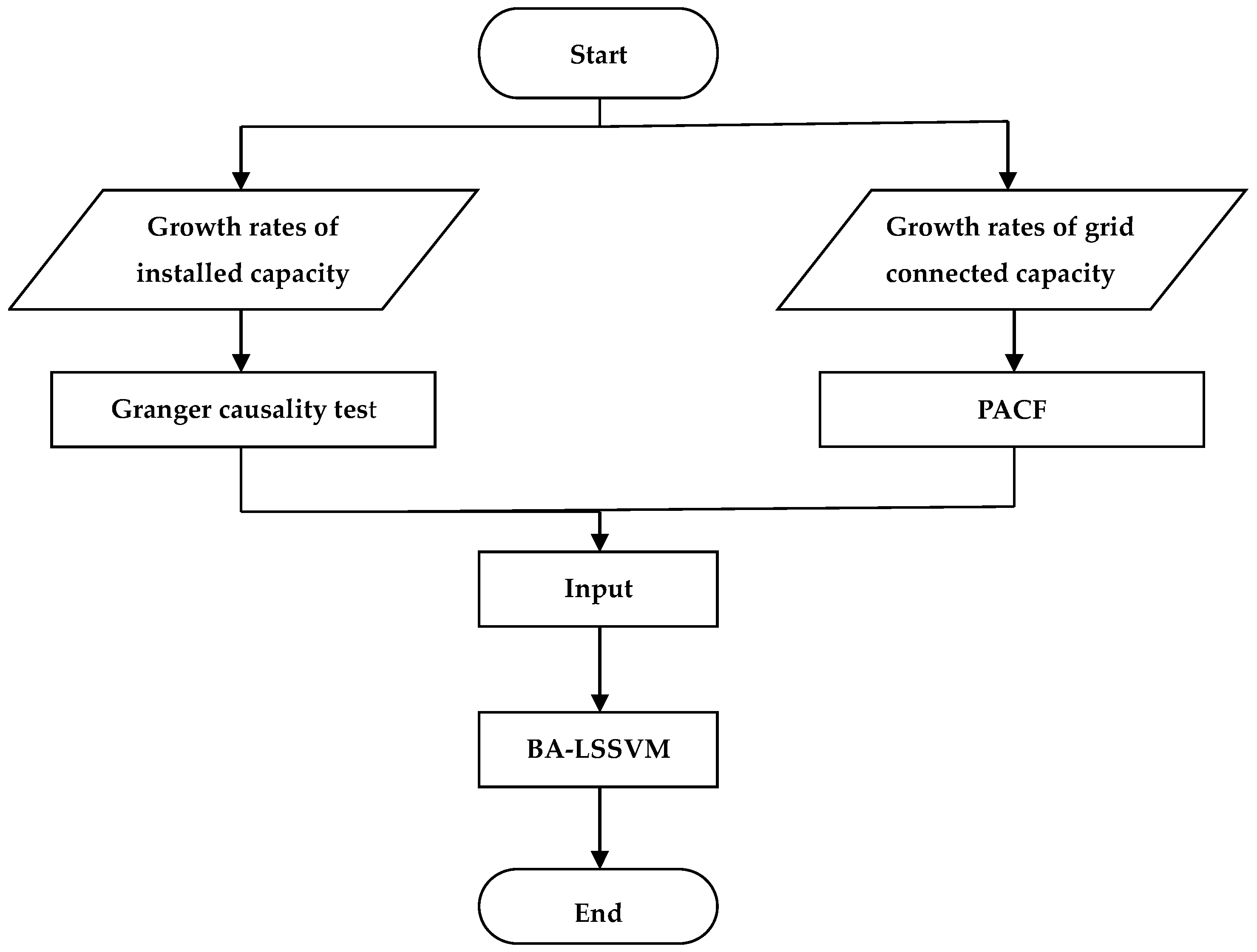
Furthermore, a wealth of variables have an impact on the forecasting accuracy and efficiency, and there has been less research looking at the input selection. These studies tend to select inputs using personal experience alone. However, in this paper, not only Stationarity, Cointegration and Granger causality tests are conducted to select the environmental factor reasonably [32], but also the partial autocorrelation analysis (PACF) is presented to calculate the lags of the growth rates of grid-connected capacity. Then, this study performed a BA-LSSVM hybrid model for wind power grid connected capacity prediction.
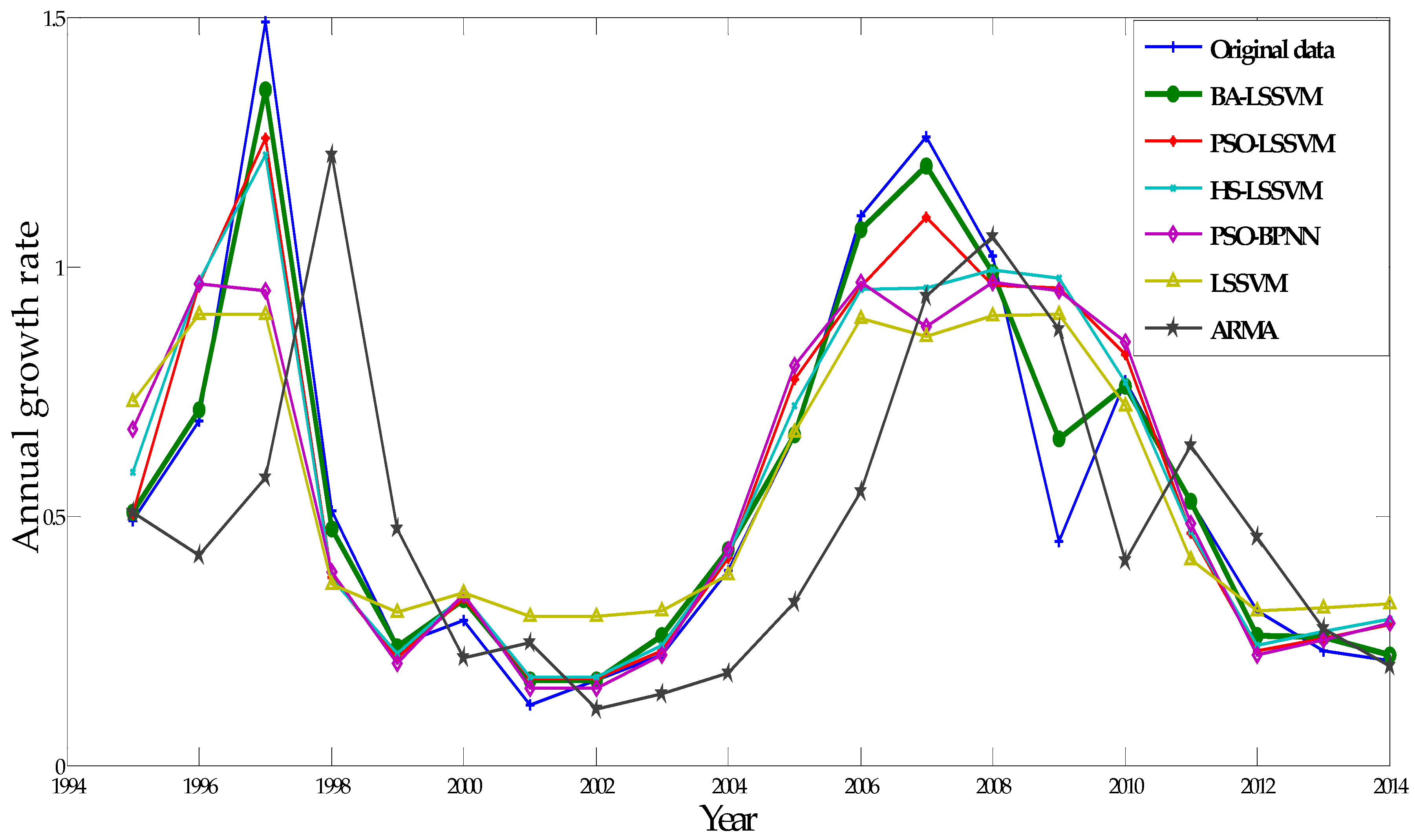
The principal purpose of this study is to investigate the accurate forecasting method of wind power capacity. In this research, a hybrid model which based on BA-LSSVM is applied. The parameters in LSSVM are fine-tuned by BA to ensure the generalization and the learning ability of LSSVM. To select the appropriate inputs, Stationarity, Cointegration and Granger causality tests and the partial autocorrelation analysis are conducted. The proposed method is simple and effective for prediction. The focus of the study is on comparing the results obtained by the BA-LSSVM, PSO-LSSVM, HS-LSSVM, PSO-BPNN, single LSSVM and ARMA models. This paper is divided into five major sections as follows. Section 2 describes the principles of BA and LSSVM respectively. In Section 3 a hybrid model is constructed which is designed to predict grid connected capacity in relation to wind power. Then, the proposed model is examined by a case study and a deep comparison of the existing methods. Finally, Section 5 provides some conclusions of the whole research.

2. Bat Algorithm (BA) and Least Squares Support Vector Machine (LSSVM)

2.1. Bat Algorithm (BA)

BA is a new meta-heuristic algorithm inspired by the echolocation behavior of bats. It provides an excellent way for the optimization and classification as its powerful selection of complicated problems [26]. The basic flow of BA can be generalized as the pseudo code listed in Algorithm 1.
Algorithm 1. Pseudo code of the Bat Algorithm.
(1) Initialize the position of bat population xi (i = 1, 2, ..., n) and vi
(2) Initialize pulse frequency fi at xi, pulse rates ri and the loudness Ai
(3) While (t < maximum number of iterations)
(4) Generate new solutions by adjusting frequency
(5) Update the velocities and solutions
(6) If (rand > ri)
(7) Select a solution among the best solutions
(8) Generate a local solution around the selected best solution
(9) End if
(10) Generate a new solution by flying randomly
(11) If (rand < Ai & f(xi) < f(x*))
(12) Accept the new solutions
(13) Increase ri and reduce Ai
(14) End if
(15) Rank the bats and find the current best x*
(16) End while

2.2. Least Squares Support Vector Machine (LSSVM)

LSSVM, proposed by Suykens [33], is an improved algorithm of support vector machine (SVM), adopting the loss function different from SVM and minimizing the square error. A quadratic programming problem is transformed into linear equations through replacing inequality constraints with equality constraints, addressing the calculation issue of large-scale data sufficiently. Figure 1 shows the flow chart of LSSVM principle.
Figure 1. The flow chart of LSSVM principle.
Energies 08 12428 g001
Then, there are two parameters, the regularization parameter and the kernel parameter, determining forecasting accuracy of the LSSVM model. In previous studies, experimental comparison, grid searching method and cross validation are optimized to the two parameters, but it is time-consuming and inefficient. Therefore, this paper adopts BA to optimize the two parameters, which can enhance and further the adaptability of the model and improve the prediction accuracy effectively.

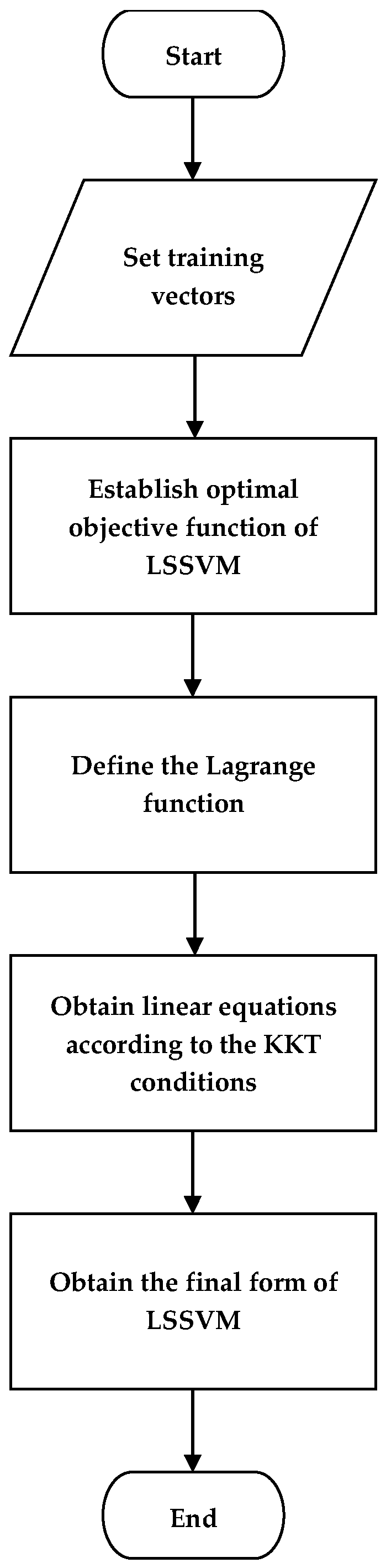
3. Bat Algorithm-Least Squares Support Vector Machine (BA-LSSVM) Approach

Based on BA-LSSVM model, the basic steps of parameter optimization can be described as follows:
(1) Parameters setting
The main parameters of BA are initial population size n, maximum iteration number N, original loudness A, pulse rate r, location vector x, speed vector v.
(2) Initialization population
Initialize the bat populations position, each bat location strategy is a component of c and σ, which can be defined as follows:
x = x min + r a n d ( 1 , d ) × ( x max x min )
where the dimension of the bat population: d = 2.
(3) Update parameters
Calculate the fitness of population, find the current optimal solution and update the pulse frequency, speed and position of bats as follows:
f i = f min + ( f max f min ) × β
v i t = v i t 1 + ( x i t x * ) × f i
x i t = x i t 1 + v i t
where β denotes uniformly random numbers, β ∈ [0,1]; fi is the search pulse frequency of the bat i, fi ∈ [fmin,fmax]; v i t and v i t 1 are the speeds of the bat i at time t and t–1, respectively; further, x i t and x i t 1 represent the location of the bat i at time t and t–1, respectively; x* is the present optimal solution for all bats.
(4) Update loudness and pulse frequency
Produce uniformly random number rand, if rand > ri, disturb the optimal strategy randomly and acquire a new strategy; if rand < Ai and f(x) > f(x*), then the new strategy can be accepted as well as the ri and Ai of the bat are updated as follows:
A i t + 1 = α A i t
r i t + 1 = r i 0 [ 1 exp ( γ t ) ]
where α and γ are constants.
(5) Output the global optimal solution
The current optimal solution can be obtained depending on the sort of all fitness values of the bat population. Repeat steps Equation (2) to Equation (4) till the maximum iterations and output the global optimal solution. Thus, a wind power grid connected capacity prediction model is performed.
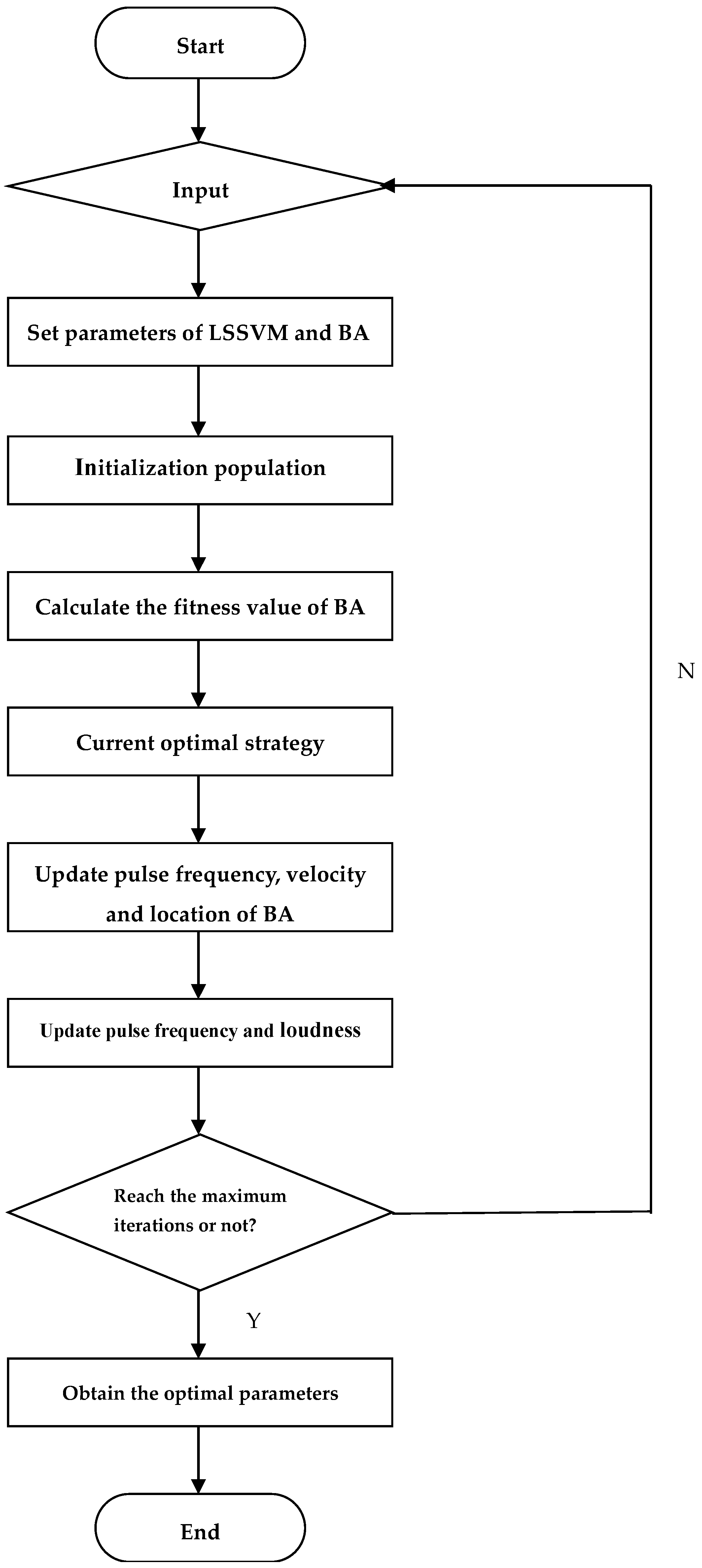
In sum, the BA-LSSVM algorithm flow chart is demonstrated in Figure 2. Firstly, LSSVM approach is employed to model the training set, and the mean square error of true value and predictive value is adopted as a fitness function of BA. Then, the group of parameter of LSSVM is optimized by BA for the minimum fitness value. Finally, the LSSVM model with optimal parameters can be applied to predict the wind power grid connected capacity.
Figure 2. The flow chart of BA-LSSVM.
Energies 08 12428 g002

4. Forecasting and Analysis of BA-LSSVM

4.1. Evaluation Indexes of Prediction Accuracy

In this article, mean square error (MSE), root mean square error (RMSE) and mean absolute error conceived as evaluation indexes are employed to assess the performance of the proposed model quantitatively:
M S E = 1 n i = 1 n ( Y i Y i ) 2
R M S E = 1 n i = 1 n ( Y i Y i Y i ) 2
M A E = 1 n i = 1 n | Y i Y i |
where n is defined as the year to be forecasted, Yi is the actual value at year i, and Y ^ i is the predictive value correspondingly.

4.2. Input Selection for Prediction Model

In this subsection, during the period of 1995–2014, newly installed capacity, cumulatively installed capacity, grid-connected capacity and cumulatively grid-connected capacity of the wind power of China are regarded as the original data. Moreover, in order to enhance forecasting accuracy, this study also formulates the growth rates of installed capacity and grid-connected capacity related to wind power. Then, to confirm the non-stationary of time series, the stationarity of each group is examined by unit root test of ADF with Lag 1, as shown in Table 1.
Table 1. Unit root test: 1995–2014.
Test MethodsInstalled Capacity of Wind PowerGrid-Connected Capacity of Wind Power
NewCumulativeGrowth RateNewCumulativeGrowth Rate
ADF test0.0987 (−3.0403)0.8264 (−3.0403)−1.8702 (−3.0403)0.2432 (−3.0403)−0.6924 (−3.0403)−2.1677 (−3.0403)
Conclusionnon-stationarynon-stationarynon-stationarynon-stationarynon-stationarynon-stationary
The null hypothesis of ADF is the existence of unit root; the critical values of significance level are indicated in parentheses; the significance level is 0.05.
According to Table 1, the ADF values of the all-time series are more than the critical value of 0.05. Thus, it can be concluded from Table 1that each time series is non-stationary. For the simplicity of dealing with the initial data, this research on grid-connected capacity forecasting of wind power could be the prediction for the annual growth rate of grid-connected capacity of wind power.
The study on the prediction for the annual growth rate of grid-connected capacity of wind power is conducted by the following steps. From previous research, it can be concluded that the input selection and the parameters have great influences on the performance of LSSVM method. Thus, this paper selects the growth rate of installed capacity belonging to the experimental variables as an exogenous variable of the growth rate of grid-connected capacity in different periods depending on a Granger causality test, and the historical data of the growth rate of grid-connected capacity are regarded as endogenous variables through calculating PACF.
In order to mine the environmental information, the correlation analysis of the growth rate of installed capacity and the growth rate of grid-connected capacity is developed appropriately. Their changes in the same year are noticeably described in Figure 3. It indicates that the growth rate of grid-connected capacity fluctuation is in line with the growth rate of installed capacity in almost years. To confirm this finding, a Granger causality test needs to be administered.
Figure 3. Relationship between the growth rate of installed capacity and the growth rate of grid-connected capacity.
Energies 08 12428 g003
Therefore, the exact causality of the two variables with various lags is explored through the Granger causality test. Granger, a Nobel Prize Winner of Economics in 2003, discovered the test approach first. The causality amongst economic variables can be analyzed in the light of the Granger causality test. One of the preconditions of the test method is the time series must be stable, otherwise it inclines to display the spurious regression issues. However, from Table 1, it seems that all-time series are non-stationary. Hence, this matter needs to be resolved by a cointegration test. The long-term information which is essential for analysis would be discarded if made stationary. In order to determine whether the two non-stationary variables have a long-term steady relationship or not, in this research, a Johansen and Juselius Cointegration test is conducted by exploiting Eviews7.2 under the Windows 7 environment. The test results are indicated in Table 2 and Table 3.
Table 2. Unrestricted Cointegration Rank Test (Trace).
HypothesizedEigenvalueTrace0.05Probability **
Number of CE(s)StatisticCritical Value
None *0.715025.979315.49470.0009
At most 10.17133.38353.84150.0658
Trace test indicates 1 cointegrating eqn(s) at the 0.05 level; * denotes rejection of the hypothesis at the 0.05 level; ** MacKinnon-Haug-Michelis (1999) p-values.
Table 3. Unrestricted Cointegration Rank Test (Maximum Eigenvalue).
HypothesizedEigenvalueTrace0.05Probability **
Number of CE(s)StatisticCritical Value
None *0.715022.595814.26460.0019
At most 10.17143.38353.84150.0658
Max-eigenvalue test indicates 1 cointegrating eqn(s) at the 0.05 level; * denotes rejection of the hypothesis at the 0.05 level; ** MacKinnon-Haug-Michelis (1999) p-values.
According to Table 3, “None” denotes the null hypothesize that there is no cointegration relationship, the trace statistic of this hypothesized is 22.5958, but the critical value of 0.05 is 14.2646. That is, the trace statistic is higher than the critical value. Therefore this finding does not support the null hypothesize, indicating there is at least one cointegration relationship. Then, “At most 1” represents the null hypothesize that there is at most one cointegration relationship, the trace statistic of this hypothesized is 3.3835, but the critical value of 0.05 is 3.8415, therefore this finding does support the null hypothesize, revealing there is one cointegration relationship.
Similarly, according to Table 4, it might be concluded that there is one cointegration relationship under the significance level of 0.05. Based on these findings, it can be concluded that the growth rate of installed capacity and the growth rate of grid-connected capacity maintain a long-term steady relationship. Therefore, implementing a Granger causality test can be reasonable. The Granger causality test results of the two non-stationary variables from Lag 1 to Lag 4 are highlighted in Table 4.
Table 4. Granger causality test for the growth rates of installed capacity and grid-connected capacity.
HypothesisLag 1Lag 2Lag 3Lag 4
GROWTH_RATE_IC does not cause GROWTH_RATE_GCC0.03640.02100.03990.0411
GROWTH_RATE_GCC does not cause GROWTH_RATE_IC0.82040.78490.15110.2812
GROWTH_RATE_IC is the growth rate of installed capacity; GROWTH_RATE_GCC is the growth rate of grid-connected capacity; the data in the Table 4 are the associated probabilities from Lag 1 to 4.
As illustrated in Table 4, according to the associated probability, under the significance level of 0.05, we can reject the null hypotheses that “GROWTH_RATE_IC does not cause GROWTH_RATE_GCC” from all lags, demonstrating that the growth rate of installed capacity affects the growth rate of grid-connected capacity. Hence, the growth rate of installed capacity can be utilized as the environmental variable for LSSVM input with the growth rate of grid-connected capacity. However, the information that “GROWTH_RATE_GCC does not cause GROWTH_RATE_IC” has less relationship with the precision of grid-connected capacity prediction, thus this study will not take the analysis of this results into consideration.
Moreover, the partial autocorrelation analysis of the growth rates of grid-connected capacity is developed to select the input of LSSVM which is associated with the forecasting data. Figure 4 describes the result of partial autocorrelation analysis where PACF represents the growth rates of grid-connected capacity. In this study, xi is set as the output variable, and xi–k can be regarded as one of the input variable when the PACF is beyond the 95% of confidence interval. From Figure 4, it is evident that the input variables for BA-LSSVM are xi, xi–1, xi–9, xi–10, xi–11.
Finally, choosing the growth rate of wind power installed capacity and the growth rate of grid connected capacity growth rate of China from 1995 to 2014 as the training set, the training model is framed, and then data from the growth rate of installed capacity about wind power from 1995 to 2014 selected as test set can be applied to acquire the forecasting values of the growth rates of grid-connected capacity in corresponding years. The overall forecasting method are constructed as shown in Figure 5.
Figure 4. The PACF of the growth rates of grid-connected capacity.
Energies 08 12428 g004
Figure 5. The overall forecasting method of BA-LSSVM.
Energies 08 12428 g005

4.3. Pretreatment Method of Original Data

The pretreatment of original data can sufficiently contribute to accelerate the training speed and convergence rate of the model. This paper effectively adopts a standardization method to reduce the prediction error of LSSVM. The pretreatment results are shown in Figure 6. And the equation of the approach can be described as follows [34]:
x i ¯ = x i x min x max x min
where x i ¯ is defined by standardized sequence value; x max and x min are the maximum and minimum of the data, respectively.
Figure 6. The pretreatment results of raw data.
Energies 08 12428 g006

4.4. BA-LSSVM Analysis Result

Previous studies on LSSVM can demonstrate that the performance of the LSSVM approach depends on its parameters. The optimization of parameters is an indispensable part of LSSVM model. BA regarded as a population intelligent optimization algorithm offers a novel idea for searching the optimal parameters of LSSVM. In this article, RBF is chosen as the kernel function of LSSVM algorithm, decreasing the complexity of the model and improving the training speed. Thus, regularization parameter c and kernel parameter σ can gain the optimal values through the powerful automatic searching ability of BA. The main parameters of BA are shown in Table 5.
Table 5. Main parameters of BA.
ParametersValuesParametersValues
Initial population size10Minimum frequency0
Initial loudness0.25Maximum frequency5
Pulse rate0.5Max-iteration number100
Using the test set, the forecasting performance of the LSSVM model with the parameters tuned by BA is examined. The errors of LSSVM are described in Figure 7. From Figure 7, it can be concluded that the error change of LSSVM is relatively steady. Only the errors of two years exceed 0.1. Furthermore, the maximum error is −0.2031 amongst all errors, implying the forecasting results are acceptable.
Figure 7. The prediction error of BA-LSSVM.
Energies 08 12428 g007

4.5. Comparative Analysis of Different Methods

To illustrate the excellent performance of the proposed algorithm, this paper employs diverse artificial intelligent algorithms to optimize the pertinent parameters of LSSVM model, including BA, PSO and HS. Meanwhile, the single LSSVM and ARMA are developed to predict the growth rate of grid-connected capacity of wind power. In addition, in this paper PSO and BP are also applied to train the neural network for forecasting. Compared with the other forecasting models, the LSSVM model based on BA displays better performance on the prediction of the growth rate of grid-connected capacity.
In this paper, the optimal parameters of all LSSVM models are shown in Table 6. Regarding the HS-LSSVM, the size of harmony memory is 10, the maximum of searching number is 100. In terms of PSO-LSSVM, the max-iteration number of PSO is 100, the size of population is 30. In addition, with respect to PSO-BPNN, the max-iteration number of PSO is 200, the number of neuron in hidden layer is 15, and the training number of BP is 300, the learning rate is 0.003. Furthermore, the time durations of the computing about different approaches are listed in Table 7. In this study, a computer equipped with an Intel® Core™ i3-3110M processor CPU @ 2.40 GHz, 4 GB RAM and the 64 bit Windows 7 operating system (OS) was used. Also, MATLAB R2014a was applied to write all programs of this paper.
Then, using various approaches with independent variables engaged in merely initial the growth rates of grid-connected capacity or the original growth rates of grid-connected capacity and the homologous growth rate of installed capacity, Figure 8 suggests the forecasting results from 1995 to 2014 in China. And, evidently the comparison of prediction results with various models is recognized in Table 8.
Table 6. The optimal parameters of LSSVM models.
ParametersForecasting Methods
BA-LSSVMPSO-LSSVMHS-LSSVMLSSVM
c 14.0350231.1334169.554774.7342
σ 0.00258.67215.15100.1267
Table 7. The time durations of the computing about different approaches.
Forecasting Methods
BA-LSSVMPSO-LSSVMHS-LSSVMPSO-BPNNLSSVMARMA
Time (s)0.92036.2202.326120.1751.4210.445
Table 8. The comparison of prediction results with different models.
IndexesForecasting Approaches
BA-LSSVMPSO-LSSVMHS-LSSVMPSO-BPNNLSSVMARMA
MSE0.02800.04360.03000.08540.08330.1279
RMSE0.09030.21330.22810.17310.28690.4120
MAE0.04060.13960.11430.14090.23820.4260
From Table 7, compared with PSO-LSSVM and HS-LSSVM, the forecasting time of BA-LSSVM is smaller, demonstrating BA can reduce the time of parameter optimization of LSSVM effectively. Moreover, the duration of computing about BA-LSSVM is lowest among all intelligent approaches.
Figure 8. The forecast results with different models.
Energies 08 12428 g008
The absolute errors between the true values and the estimated values may be captured according to Figure 8. ARMA has poor performance on forecasting the growth rate of grid-connected capacity, since the deviation of ARMA is the highest among the six methods. In contrast, the prediction values obtained in almost years by BA-LSSVM can be acceptable. Furthermore, in comparison with the single LSSVM model, the hybrid models of LSSVM with the parameters optimized by intelligent algorithms have great advantages in prediction of the growth rate of grid-connected capacity. Most importantly, the BA-LSSVM method outperforms other improved LSSVM models.
From Table 8, the following conclusions may be reached: (a) this study establishes three improved LSSVM models, and the performance of LSSVM based on BA is superior to the HS-LSSVM and the PSO-LSSVM with respect to the evaluation indexes of MSE, RMSE and MAE. For instance, the MSE of the BA-LSSVM is 0.0280, but the PSO-LSSVM and HS-LSSVM are 0.0300 and 0.0436, respectively; the MAE of the BA-LSSVM is 0.0406, but the PSO-LSSVM and the HS-LSSVM are 0.1396 and 0.1143, respectively. There is a paramount reason for this phenomenon, namely that BA adopts the major advantages of the existing intelligent algorithms in some way, combining the amazing echolocation behavior of bats, while PSO and HS are special cases of the BA in simplified forms; (b) the improved LSSVM models have better performance than single LSSVM approach. The primary reason may be the improved LSSVM model is added to the process of automatic searching, which equips the LSSVM model with better learning and generalization ability to acquire the global optimal solution easily; (c) the improved LSSVM approaches have higher accuracy than PSO-BPNN in relation to the evaluation criteria. For instance, the MAE of the PSO-BPNN is 0.1409, but the BA-LSSVM, the PSO-LSSVM and the HS-LSSVM are 0.0406, 0.1396 and 0.1143, respectively. This might be accounted for by inability of BPNN to obtain the global optimal solution. A possible explanation may be that the neural network utilizes the gradient descent method to optimize the weights, and the optimization process can only be guaranteed to converge to one of the points. Besides, the RMSE of PSO-BPNN is lower than PSO-LSSVM, HS-LSSVM. A explanation might be that PSO-BPNN emphasize the RMSE taken as the sole fitness criterion while it neglects the other indexes; (d) compared with the ARMA model which merely utilizes its own historical data, the improved LSSVM methods and the hybrid neural network model (PSO-BPNN) are more powerful than the ARMA model, which proves that the intelligent approaches have more research value and development space than the statistical models in the area of forecasting.

5. Conclusions

In order to forecast the grid-connected capacity of wind power efficiently, a hybrid model is framed in this study. Firstly, Stationarity, Cointegration, Granger causality tests and PACF are employed to select the input of LSSVM method. Then, the regularization parameter c and kernel parameter σ of the proposed models are optimized by BA. Finally, the presented method with favorable learning ability and generalization is applied to predict the growth rate of grid-connected capacity of wind power.
According to the different prediction algorithms and the three evaluation indexes, the following conclusions may be drawn: (a) the hybrid LSSVM models and the pure LSSVM model outperform ARMA; (b) the different criteria of the BA-LSSVM are minimum in comparison with PSO-LSSVM and HS-LSSVM; (c) The improved LSSVM approaches have higher forecasting accuracy than PSO-BPNN. The exciting results demonstrate that the accuracy improvement of the BA-LSSVM can reach about 20%, which indicates the current method is a very promising algorithm for wind power grid connected capacity prediction.
Regarding some limitations of this study, further research is necessary. First, this study only selected installed capacity as an exogenous variable of the growth rate of grid-connected capacity, thus the other relevant factors that affect the grid-connected capacity are needed to investigate in further research.
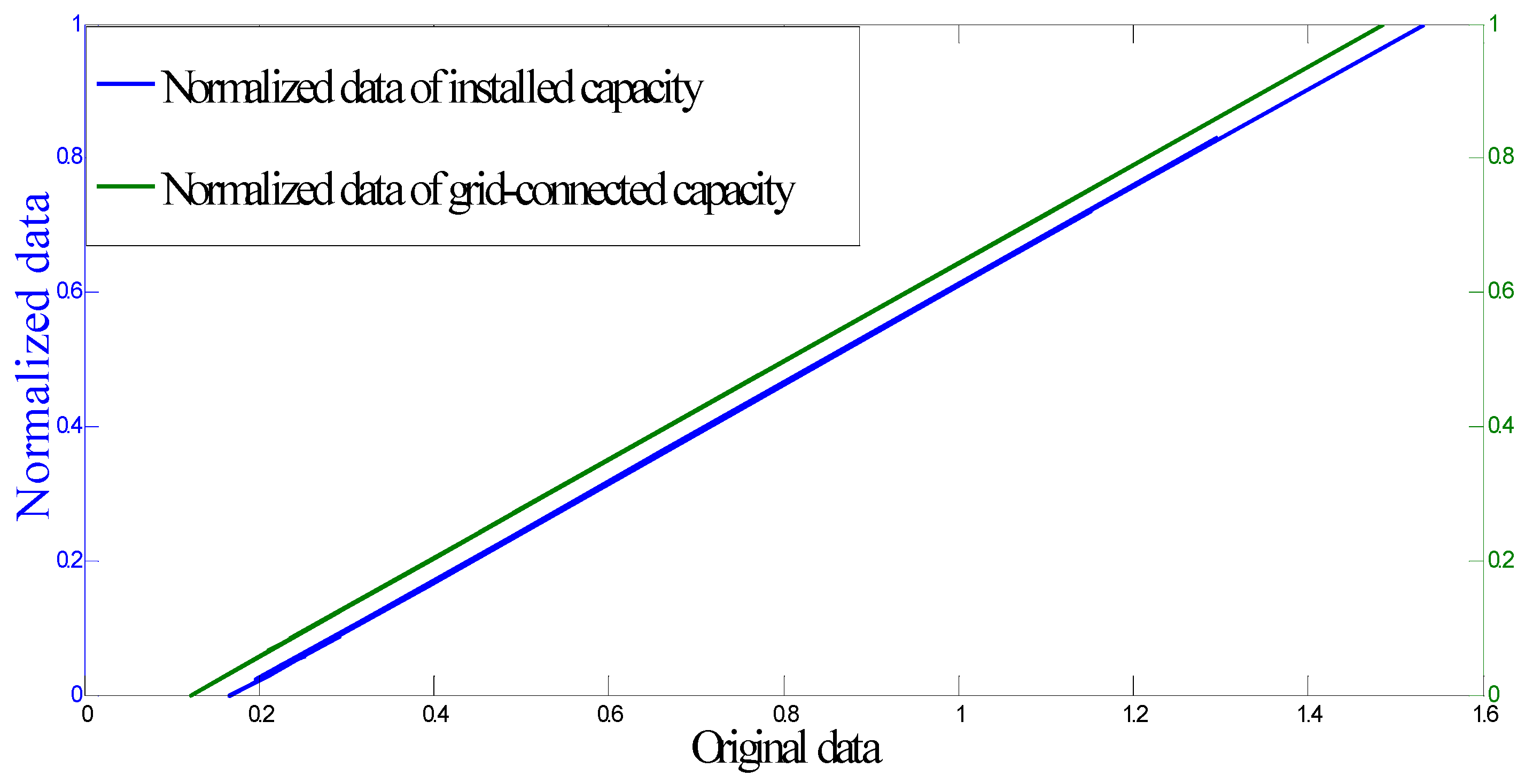
Second, in this paper a normalized method were adopted to reduce the prediction error of LSSVM. To enhance forecasting accuracy further, future studies need to explore more effective approach of data processing.

Acknowledgments

This study is supported by Soft Science Research Base of Hebei Province and Philosophy and Social Science Research Base of Hebei Province.

Author Contributions

Qunli Wu designed this paper and made overall guidance; Chenyang Peng wrote the whole manuscript. All authors read and agreed to the final article.

Conflicts of Interest

The authors declare no conflict of interest.

References

  1. Xu, J.; He, D.; Zhao, X. Status and prospects of chinese wind energy. Energy 2010, 35, 4439–4444. [Google Scholar] [CrossRef]
  2. Foley, A.M.; Leahy, P.G.; Marvuglia, A.; McKeogh, E.J. Current methods and advances in forecasting of wind power generation. Renew. Energy 2012, 37, 1–8. [Google Scholar] [CrossRef] [Green Version]
  3. Jin, X.; Zhang, Z.; Shi, X.; Ju, W. A review on wind power industry and corresponding insurance market in china: Current status and challenges. Renew. Sustain. Energy Rev. 2014, 38, 1069–1082. [Google Scholar] [CrossRef]
  4. Zou, J.; Peng, C.; Yan, Y.; Zheng, H.; Li, Y. A survey of dynamic equivalent modeling for wind farm. Renew. Sustain. Energy Rev. 2014, 40, 956–963. [Google Scholar] [CrossRef]
  5. Ahmed, H. Reactive power and voltage control in grid-connected wind farms: An online optimization based fast model predictive control approach. Electr. Eng. 2015, 97, 35–44. [Google Scholar] [CrossRef]
  6. Ewing, B.T.; Kruse, J.B.; Schroeder, J.L.; Smith, D.A. Time series analysis of wind speed using var and the generalized impulse response technique. J. Wind Eng. Ind. Aerodyn. 2007, 95, 209–219. [Google Scholar] [CrossRef]
  7. Hill, D.; Bell, K.R.W.; McMillan, D.; Infield, D. A vector auto-regressive model for onshore and offshore wind synthesis incorporating meteorological model information. Adv. Sci. Res. 2014, 11, 35–39. [Google Scholar] [CrossRef] [Green Version]
  8. Torres, J.L.; García, A.; de Blas, M.; de Francisco, A. Forecast of hourly average wind speed with arma models in Navarre (Spain). Sol. Energy 2005, 79, 65–77. [Google Scholar] [CrossRef]
  9. Erdem, E.; Shi, J. Arma based approaches for forecasting the tuple of wind speed and direction. Appl. Energy 2011, 88, 1405–1414. [Google Scholar] [CrossRef]
  10. Liu, H.; Erdem, E.; Shi, J. Comprehensive evaluation of ARMA–GARCH(-M) approaches for modeling the mean and volatility of wind speed. Appl. Energy 2011, 88, 724–732. [Google Scholar] [CrossRef]
  11. Jiang, W.; Yan, Z.; Feng, D.-H.; Hu, Z. Wind speed forecasting using autoregressive moving average/generalized autoregressive conditional heteroscedasticity model. Eur. Trans. Electr. Power 2012, 22, 662–673. [Google Scholar] [CrossRef]
  12. Tagliaferri, F.; Viola, I.M.; Flay, R.G.J. Wind direction forecasting with artificial neural networks and support vector machines. Ocean Eng. 2015, 97, 65–73. [Google Scholar] [CrossRef]
  13. Buhan, S.; Cadirci, I. Multistage wind-filectric power forecast by using a combination of advanced statistical methods. IEEE Trans. Ind. Inform. 2015, 11, 1231–1242. [Google Scholar] [CrossRef]
  14. Shukur, O.B.; Lee, M.H. Daily wind speed forecasting through hybrid kf-ann model based on arima. Renew. Energy 2015, 76, 637–647. [Google Scholar] [CrossRef]
  15. Ata, R. Artificial neural networks applications in wind energy systems: A review. Renew. Sustain. Energy Rev. 2015, 49, 534–562. [Google Scholar] [CrossRef]
  16. Petkovic, D.; Shamshirband, S.; Anuar, N.B.; Naji, S.; Kiah, M.L.M.; Gani, A. Adaptive neuro-fuzzy evaluation of wind farm power production as function of wind speed and direction. Stoch. Environ. Res. Risk Assess. 2015, 29, 793–802. [Google Scholar] [CrossRef]
  17. Zhang, Y.; Yang, J.; Wang, K.; Wang, Z. Wind power prediction considering nonlinear atmospheric disturbances. Energies 2015, 8, 475–489. [Google Scholar] [CrossRef]
  18. Guo, Z.H.; Zhao, J.; Zhang, W.Y.; Wang, J.Z. A corrected hybrid approach for wind speed prediction in Hexi Corridor of China. Energy 2011, 36, 1668–1679. [Google Scholar] [CrossRef]
  19. De Giorgi, M.; Campilongo, S.; Ficarella, A.; Congedo, P. Comparison between wind power prediction models based on wavelet decomposition with least-squares support vector machine (LS-SVM) and artificial neural network (ANN). Energies 2014, 7, 5251–5272. [Google Scholar] [CrossRef]
  20. Yuan, X.; Chen, C.; Yuan, Y.; Huang, Y.; Tan, Q. Short-term wind power prediction based on LSSVM–GSA model. Energy Convers. Manag. 2015, 101, 393–401. [Google Scholar] [CrossRef]
  21. Wang, X.; Li, H. One-month ahead prediction of wind speed and output power based on EMD and LSSVM. In Proceedings of the International Conference on Energy and Environment Technology, Guilin, China, 16–18 October 2009; pp. 439–442.
  22. Hu, Z.Y.; Liu, Q.Y.; Tian, Y.X.; Liao, Y.F. A short-term wind speed forecasting model based on improved QPSO optimizing LSSVM. In Proceedings of the International Conference on Power System Technology (POWERCON), Chengdu, China, 20–22 October 2014.
  23. Sun, B.; Yao, H.T. The short-term wind speed forecast analysis based on the PSO-LSSVM predict model. Power Syst. Prot. Control 2012, 40, 85–89. [Google Scholar]
  24. Wang, J.Z.; Wang, Y.; Jiang, P. The study and application of a novel hybrid forecasting model—A case study of wind speed forecasting in china. Appl. Energy 2015, 143, 472–488. [Google Scholar] [CrossRef]
  25. Song, Z.; Li, J. Prediction model based on least squares support vector machine with harmony search and its application. J. Harbin Inst. Technol. 2009, 41, 208–210. [Google Scholar]
  26. Yang, X.-S. A new metaheuristic bat-inspired algorithm. Nat. Inspir. Coop. Strateg. Optim. 2010, 284, 65–74. [Google Scholar]
  27. Hafezi, R.; Shahrabi, J.; Hadavandi, E. A bat-neural network multi-agent system (BNNMAS) for stock price prediction: Case study of dax stock price. Appl. Soft Comput. 2015, 29, 196–210. [Google Scholar] [CrossRef]
  28. Meng, X.B.; Gao, X.Z.; Liu, Y.; Zhang, H.Z. A novel bat algorithm with habitat selection and doppler effect in echoes for optimization. Expert Syst. Appl. 2015, 42, 6350–6364. [Google Scholar] [CrossRef]
  29. Senthilkumar, P.; Vanitha, N.S. A unified approach to detect the record duplication using bat algorithm and fuzzy classifier for health informatics. J. Med. Imaging Health Inform. 2015, 5, 1121–1132. [Google Scholar] [CrossRef]
  30. Rao, B.V.; Nagesh Kumar, G.V. Optimal power flow by bat search algorithm for generation reallocation with unified power flow controller. Int. J. Electr. Power Energy Syst. 2015, 68, 81–88. [Google Scholar]
  31. Yang, N.C.; Le, M.D. Optimal design of passive power filters based on multi-objective bat algorithm and pareto front. Appl. Soft Comput. 2015, 35, 257–266. [Google Scholar] [CrossRef]
  32. Tang, C.F.; Tan, E.C. Electricity consumption and economic growth in Portugal: Evidence from a multivariate framework analysis. Energy J. 2012, 33, 23–48. [Google Scholar]
  33. Suykens, J.A.K.; Vandewalle, J. Recurrent least squares support vector machines. IEEE Trans. Circuits Syst. I Fundam. Theory Appl. 2000, 47, 1109–1114. [Google Scholar] [CrossRef]
  34. Ahmed, H.; Ushirobira, R.; Efimov, D.; Tran, D.; Sow, M.; Payton, L.; Massabuau, J.C. A fault detection method for automatic detection of spawning in oysters. IEEE Trans. Control Syst. Technol. 2015. [Google Scholar] [CrossRef]

