
Rotor Design for Diffuser Augmented Wind Turbines

Volu Ventis ApS, Ferskvandscentret, 8600 Silkeborg, Denmark
*
Author to whom correspondence should be addressed.
Energies 2015, 8(10), 10736-10774; https://doi.org/10.3390/en81010736
Submission received: 2 July 2015
/
Revised: 11 September 2015
/
Accepted: 21 September 2015
/
Published: 28 September 2015
(This article belongs to the Special Issue Wind Turbine 2015)
Abstract
:Diffuser augmented wind turbines (DAWTs) can increase mass flow through the rotor substantially, but have often failed to fulfill expectations. We address high-performance diffusers, and investigate the design requirements for a DAWT rotor to efficiently convert the available energy to shaft energy. Several factors can induce wake stall scenarios causing significant energy loss. The causality between these stall mechanisms and earlier DAWT failures is discussed. First, a swirled actuator disk CFD code is validated through comparison with results from a far wake swirl corrected blade-element momentum (BEM) model, and horizontal-axis wind turbine (HAWT) reference results. Then, power efficiency versus thrust is computed with the swirled actuator disk (AD) code for low and high values of tip-speed ratios (TSR), for different centerbodies, and for different spanwise rotor thrust loading distributions. Three different configurations are studied: The bare propeller HAWT, the classical DAWT, and the high-performance multi-element DAWT. In total nearly 400 high-resolution AD runs are generated. These results are presented and discussed. It is concluded that dedicated DAWT rotors can successfully convert the available energy to shaft energy, provided the identified design requirements for swirl and axial loading distributions are satisfied.
1. Introduction
Wind energy today has become the most significant provider of renewable energy. This is the outcome of a reliable robust concept, and the commercial feasibility for up-scaling the 3-bladed lift-driven front-runner “Danish concept” to large wind applications approaching 10 MW in rated capacity. In the other end of the size range, small wind is represented by a variety of technologies, including HAWTs, DAWTs, VAWTs, back-runners, and drag-driven WTGs. The driver for this diversity is the very different set of design constraints for small wind, and in particular for household turbines. They should not be visually obtrusive and rotating parts are generally not favored, although hard to avoid. Inaudible operation is also an attractive small-wind feature, as is compactness, failure mode safety, and design simplicity. Most household turbines power interface to the grid. Simple battery storage of a DC-output is an attractive alternative, due to the rapid recent advances in electrical energy storage. An end-consumer (household) energy storage capacity could be an essential part of a smart-grid, constituting an energy buffer for excess capacity during windy and/or sunny days from both sides of the electricity meter: household renewable as well as community energy sources.
As a candidate for household turbines, we focus our attention to DAWTs. Their virtues are: visual shielding of rotating parts, compact energy capture, and silent operation provided that the tip speed is kept low. However, DAWTs have a troubled past, where power performance expectations have not been met, leading to unfulfilled Cost-of-Energy (CoE) predictions. DAWT Research has been conducted on an academic and industrial level, somewhat sporadically, for decades [1,2,3,4,5,6,7,8,9,10,11], leading to later commercial attempts to exploit the technology large-scale, e.g., by Vortec Energy Limited and more recently by Ogin Energy (formerly FloDesign Wind Turbines). Comprehensive coverage of the DAWT history is given in [12]. DAWT aerodynamic theory is more complex than for bare propeller HAWTs due to the Venturi effect created by the diffuser (or shroud) surrounding the rotor. 1D momentum theory for regular actuator disks [13] and the BEM model [14,15] for spinning rotors predict the performance of HAWTs with good accuracy, considering the simplicity of these models. BEM is the cornerstone of HAWT design and evaluation, and various add-on modules have been devised during the last 3 decades to further enhance the BEM model accuracy and applicability. Therefore, efforts have been made to generalize the 1D momentum theory and/or BEM model and make it applicable to DAWTs as well. The contributions by van Bussel [16,17], Jamieson [18], Werle and Pretz [19], and Hjort and Larsen [20] fall into this category. Jamieson and Werle and Pretz reach similar results. Both identify the speed-up factor of the axial velocity through the rotor disk at zero thrust as the augmentation factor of the available power efficiency. Werle and Pretz further identify the proportionality shroud coefficient between the axial force on the diffuser and the rotor thrust to equal the speed-up factor at zero power take-out minus one. Hjort and Larsen relax the earlier applied 1D-assumption such that the diffuser-induced speed-up at the rotor plane is no longer constant but is allowed to vary radially, leading to rotor area-averaged but otherwise quite similar expressions. They also show that Werle and Pretz’ shroud coefficient can only be regarded as constant in the linear proximity of the zero-thrust operational point, and demonstrate through AD CFD analysis that this linear range is very limited, and consequently that the zero-power axial velocity speed-up factor is only useful for DAWT optimization as a crude first-order approximation. Hansen [21] also noted that a proper DAWT diffuser should be designed for maximum power take-out under loaded conditions. This limits the scope of the zero-thrust speed-up factor as a design parameter for DAWT optimal power prediction.
Acknowledging that BEM methods for DAWTs are approximate, and increasingly so under power-optimal loaded conditions, Hjort and Larsen [20] used a much more general AD CFD model to optimize a very efficient and compact multi-element DAWT diffuser under optimally loaded conditions. The reported available power coefficient based on diffuser exit area, , was 1.49 times Betz (16/27) and the available power coefficient based on rotor area, , was 2.77 times Betz. With “available power” we mean the power that is taken out by an ideal actuator disk. The ideal actuator disk is characterized by these assumptions:
- Infinite tip-speed ratio, λ.
- Infinite rotor blade lift-over-drag ratio, L/D.
- No centerbody (nacelle).
The present investigation proceeds one step further and addresses the adequate design of a rotor, including centerbody, for the multi-element diffuser, and high performance diffusers in general, aiming at maximizing the shaft energy power coefficient and thereby the rotor efficiency. The non-ideal actuator disk is characterized by having:
- Finite realistic tip-speed ratio, λ.
- Finite realistic rotor blade lift-over-drag ratio, L/D.
- A centerbody (nacelle).
In comparison, rotor design for a bare propeller HAWT is a trivial task with a standard BEM. By contrast, the task is non-trivial in the case of a DAWT. This is a fact which is probably best evidenced by the failures of the past, and for that reason we base this investigation on a higher-complexity tool such as the AD CFD axisymmetric model with swirl. The objective is to derive the best possible DAWT rotor design approach, and to identify possible aerodynamic failure modes that might help explain why earlier attempts to obtain high power augmentation have generally failed.
This paper is organized as follows: In Section 2 the basic momentum theory for a swirled flow field governing the HAWT is presented. Special attention is given to the often excluded term containing the impact of far wake rotation, and its implication on the radial element independence property for the BEM formulation. Section 3 derives the actuator disk (AD) CFD volume forces that are identical to the BEM disk forces from Section 2. The AD results for a bare propeller HAWT are then validated against the BEM results. The validated AD CFD code is then used to compute several hundred different cases with varying diffuser configuration, rotor thrust loading, TSR, centerbody, and spanwise loading distribution, which are presented and discussed in Section 4. Special focus is on how to ensure proper energy capture without suffering power-losses so often associated with DAWTs. Section 5 concludes this study and outlines perspectives and limitations for DAWTs with dedicated rotor designs.
2. A Simple BEM Formulation for HAWTs with Full Inclusion of Swirl Effects
The following BEM formulation will have two distinctive features: inclusion of the far-wake pressure loss term, and the non-iterative solution strategy for ideal rotors with no blade drag forcing. Otherwise, the formulation is standard.
2.1. BEM Derivation
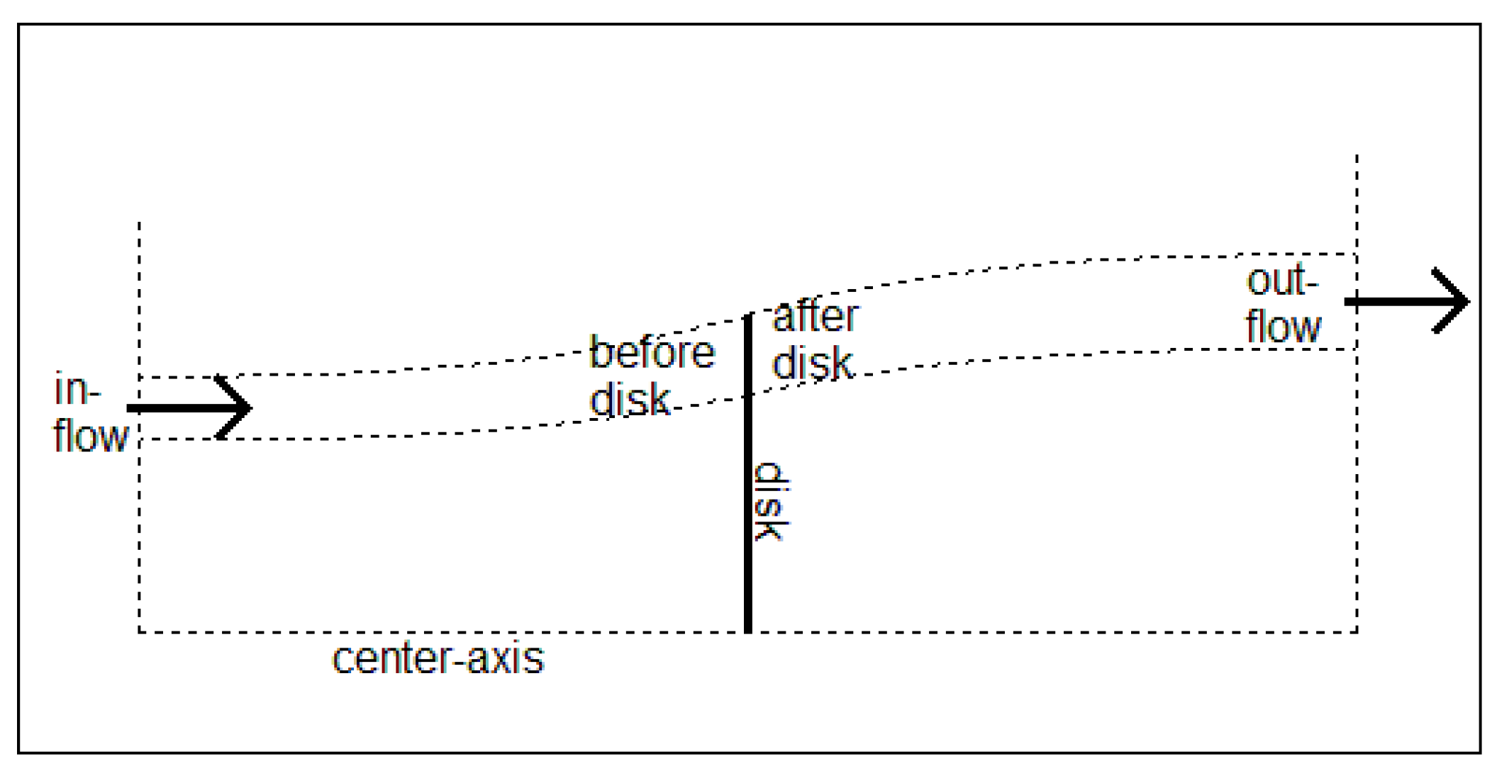
A control volume for a stream tube element is defined by the dividing streamlines, the flow inlet and the flow outlet, see Figure 1. The domain is axisymmetric in the direction perpendicular to the plane. The actuator disk is indexed “d”, across which there is a pressure drop, pd+ – pd–. The variables of each of the four flow states are listed in Table 1 for an arbitrary i’th stream tube.
Figure 1.
Horizontal-axis wind turbine (HAWT) control volume of a radial element (stream tube). The wake part of the element is marked by the streamlines emanating downstream of the disk in the center. Inflow is assumed far upstream, and outflow is assumed far downstream in the fully developed wake.


| State | Stream Tube Area | Static Pressure | Axial Velocity | Azimuthal Velocity |
|---|---|---|---|---|
| inflow | ||||
| before disk | ||||
| after disk | ||||
| outflow |
The flow is governed by the incompressible Navier-Stokes equations. Steady conditions are assumed. Viscous effects can be included as drag forcing in the interaction between the rotor blades (i.e., the disk) and the passing flow, but are otherwise neglected upstream and downstream of the rotor disk. The fully developed far wake will be aligned with the free stream and thus have zero velocity gradients in the radial direction, ∂/∂r = 0 and being axisymmetric, ∂/∂θ = 0. The inviscid steady incompressible Navier Stokes (NS) equations in the far wake, expressed in cylindrical coordinates, then reduce to a simple relation between the radial pressure gradient and the swirl velocity component in the azimuthal direction.
Outside the far wake the pressure is ambient and with no swirl. This provides a boundary condition for Equation (1), so the far wake pressure drop due to rotation can be found by integration as follows.
The flow across the disk in Figure 1 is characterized by a pressure drop, pd+ – pd–, and the onset of azimuthal (swirl) flow velocity, caused by the forces exerted by the rotor disk onto the passing flow in the axial and azimuthal directions. We consider a control volume bounded axially far upstream and far downstream, and bounded radially by an inner and outer stream sheet (stream lines in 2D, e.g., on Figure 1) extending circumferentially in an axisymmetric manner, such that each control volume has the form of a tube expanding radially in the vicinity of the disk but otherwise constant in cross-section far upstream and far downstream. The radial element dependency introduced by the far wake pressure term should be kept in mind, although the functional dependency on radius, r, is skipped in notion for brevity, . The derivation below holds for an arbitrary i’th tube element, where index ‘i’ as used in Table 1 has been omitted for clarity.
Conservation of momentum inside a tube-element control volume in the axial direction is expressed as follows:
Initially, we shall assume an ideal rotor with negligible drag losses corresponding to Figure 2a.
Figure 2.
Display of axial and tangential flow components as seen from the rotating blades’ reference. The forces exerted by the rotating blades on the fluid are shown. (a) Ideal blade with no drag force; (b) Drag force included (drag force magnitude exaggerated for visual clarity).
Figure 2.
Display of axial and tangential flow components as seen from the rotating blades’ reference. The forces exerted by the rotating blades on the fluid are shown. (a) Ideal blade with no drag force; (b) Drag force included (drag force magnitude exaggerated for visual clarity).
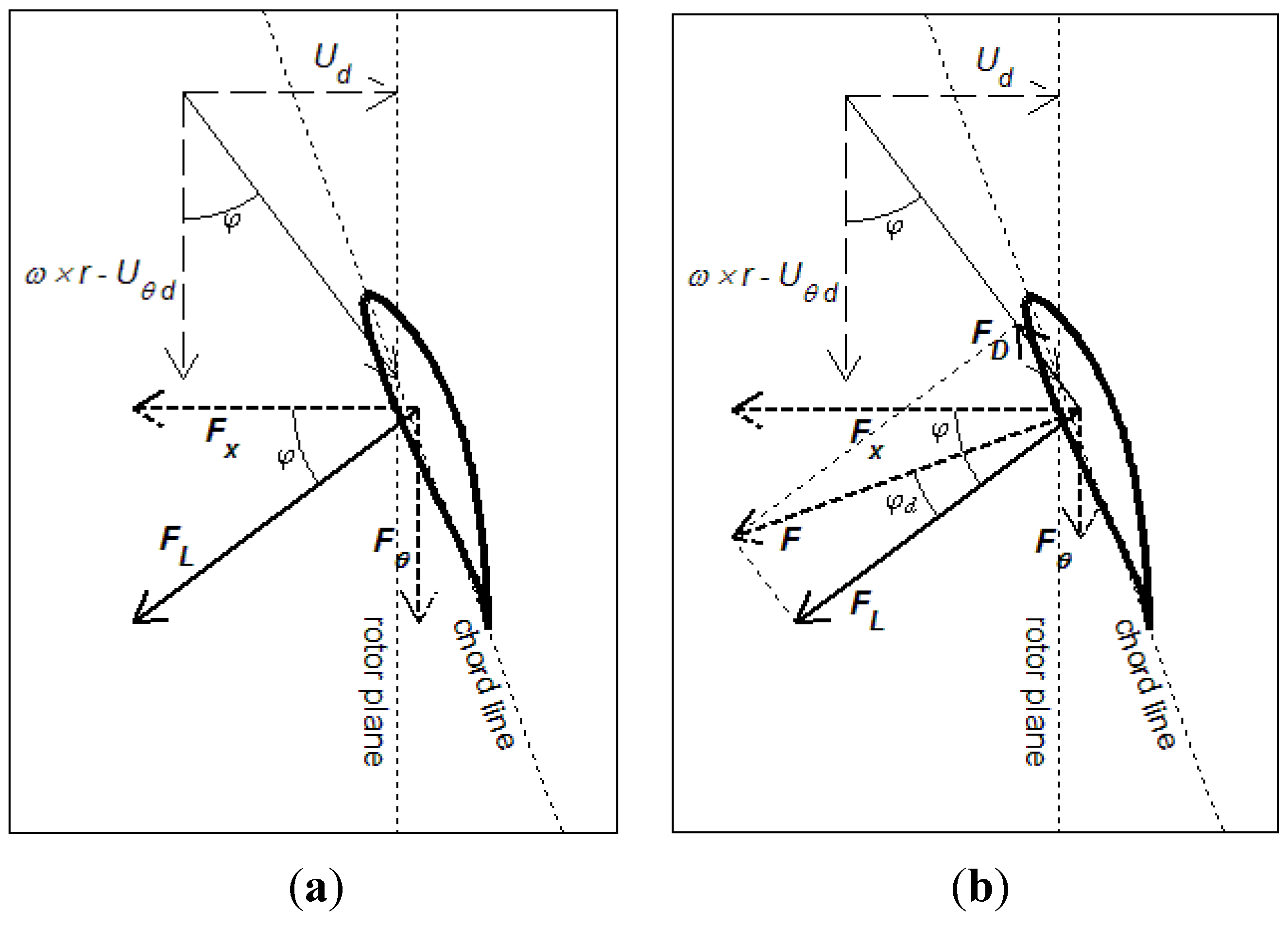
Fx is the disks axial thrust force on the fluid, and is positive when power is taken out of the flow (wind turbine mode). Conservation of momentum inside a tube-element control volume in the azimuthal direction gives:
Fθ is the disk’s azimuthal (tangential) force on the fluid, and is positive having the opposite sign of the azimuthal velocity component, Uθw. The relation between the disk forces Fx and Fθ is determined primarily by the tip-speed-ratio (TSR) of the rotating disk.
where Uθd is defined as the azimuthal velocity component at the streamwise center of the rotor disk where half of the azimuthal forcing from the disk on the passing air has taken place. Since the azimuthal flow velocity inside a tube-element can only be impacted by the disk, the relation between azimuthal velocity at the disk streamwise center and the far wake is simply:
Conservation of mass along a tube-element gives:
Bernouilli’s Equation applied along a streamline upstream of the disk:
Bernouilli’s Equation applied along a streamline downstream of the disk:
Equations (2)–(10) constitute the simple BEM formulation with full inclusion of swirl effects. The far wake pressure term, Δpw, expressed by Equation (2) is neglected in the standard BEM formulation [15], since the attractive property of tube-element independency is then retained. Madsen et al. [22] identified the same missing pressure term, i.e., Equation (2), in their investigation and showed how the full inclusion of far-wake rotational effects helped improve the match between BEM results and AD CFD results. In an attempt to include the tube-element independency while still addressing the far wake pressure term, Burton et al. [23] approximated the term as the pressure head loss due to far wake rotation, giving the simplified but radially independent expression: . The modeling accuracy from use of Burton’s approximated term instead of the radially dependent term from Equation (2) is quantified and discussed in Section 3.
The reduction of variables for Equations (2)–(10) is shown in Appendix 1. Due to the simplified relation between axial and azimuthal forcing from the rotor expressed in Equation (5), the far wake axial velocity could be computed analytically without resorting to numerical iterations, if the far wake pressure term were neglected. Including the far wake pressure term yields:
In the above equation Uθw is treated as the RHS free variable enabling the computation of the LHS Uw Once Uθw and Uw are known, the remaining unknowns, Ud, Uθd, pd+, pd– and Δpw are readily found by insertion. When the far wake pressure term Δpw is included, an iterative approach is necessary. A simple iterative scheme for solving Equation (11) is described in Appendix 1.
The thrust and power coefficients for each tube element are defined as:
where lower-case velocities denote normalization with the free stream velocity, .
Note that the power coefficient is conveniently decomposed into the normalized rate of work done by the axial forces and the azimuthal forces respectively:
The correct quantification of the work done by the fluid on the rotor is very important. In the absence of viscosity effects on the rotor (no drag), the rotor’s work on the wind, Equations (13)–(15), equals the magnitude of the wind’s work on the rotor, Equations (17)–(19), because no mechanical energy is lost in the force action/re-action between the wind and the rotor. In the presence of viscosity effects on the rotor (drag), the transfer of mechanical energy is no longer ideal, and Equations (13)–(15) would have to include a viscous loss term.
The axial power coefficient, , is positive since the axial force from the AD on the fluid and the axial fluid velocity through the AD are oppositely signed, such that the reaction force –Fx exerted by the fluid on the AD is co-directional with Ud. By contrast, the azimuthal power coefficient, , is negative since the azimuthal force from the AD on the fluid and the azimuthal fluid velocity through the AD are equally signed, such that the reaction force –Fθ exerted by the fluid on the AD is contra-directional with Uθd. Again, Equations (12)–(15) are valid only for ideal disks with no drag.
The drag force from the blades on the fluid can be included as depicted in Figure 2b. The now finite L/D ratio leads to a modified expression for the relation between axial and azimuthal forcing from the disk on the fluid. The modified Equation (5) and the consequent introduction of an extra term to be computed iteratively is shown and discussed in Appendix 1. A consequence of introducing drag forcing is that the magnitude of the disk’s mechanical work on the fluid no longer equals the fluid’s mechanical work on the disk, since some of the disk’s work on the fluid is converted to heat through viscosity. Therefore, Equations (12)–(15) must be expressed in more general terms for finite L/D ratios. Forces and angles are sketched on Figure 2.
and are the power efficiencies delivered by the airfoil lift force and drag force respectively. The lift- and drag-coefficients are conveniently expressed as a function of axial thrust forcing Fx, the local flow quantities at the disk, and the L/D ratio:
2.2. BEM Results
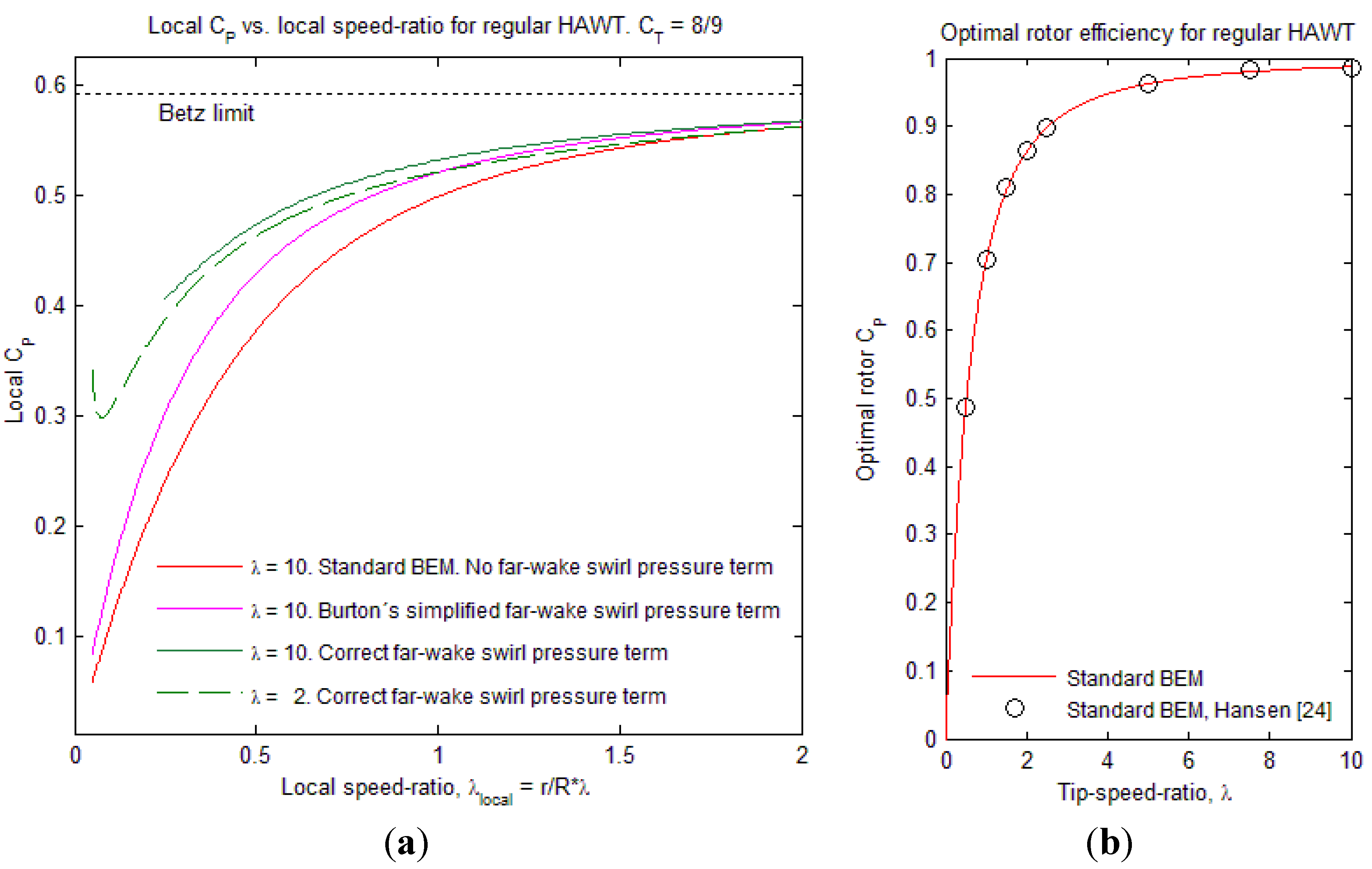
The eventual inclusion of the far-wake swirl pressure term has an impact when swirl is pronounced, i.e., at low speed-ratios. The reason for our interest in slowly rotating rotors will become evident in Section 4.
Figure 3a, shows the wake-loss for the ideal rotor disk (no drag) due to the work done by the tangential disk forces on the fluid, causing swirl. The wake loss is most severe for the simpler BEM version. Differences in local Cp become significant at local speed-ratios below approximately 1. Figure 3b has validation purpose and shows rotor-integrated optimal power efficiency as a function of TSR for the standard BEM, which is in excellent agreement with the well-known Glauert results in Table 4.2 of Hansen [24].
Figure 3.
(a) Local power efficiency versus local speed-ratio at a tip-speed ratio (TSR) of 10 for three different treatments of the far-wake pressure term. Note that only the local speed-ratio matters for the two blade-element momentum (BEM) versions with tube element independency (Standard BEM, BEM with simplified far-wake pressure term). Tube element independency is sacrificed in the present BEM with correct far-wake pressure term. This is why the local Cp changes slightly when the TSR is reduced from 10 to 2 (green curves); (b) Comparison of standard BEM results for optimal rotor Cp with ref. [24].

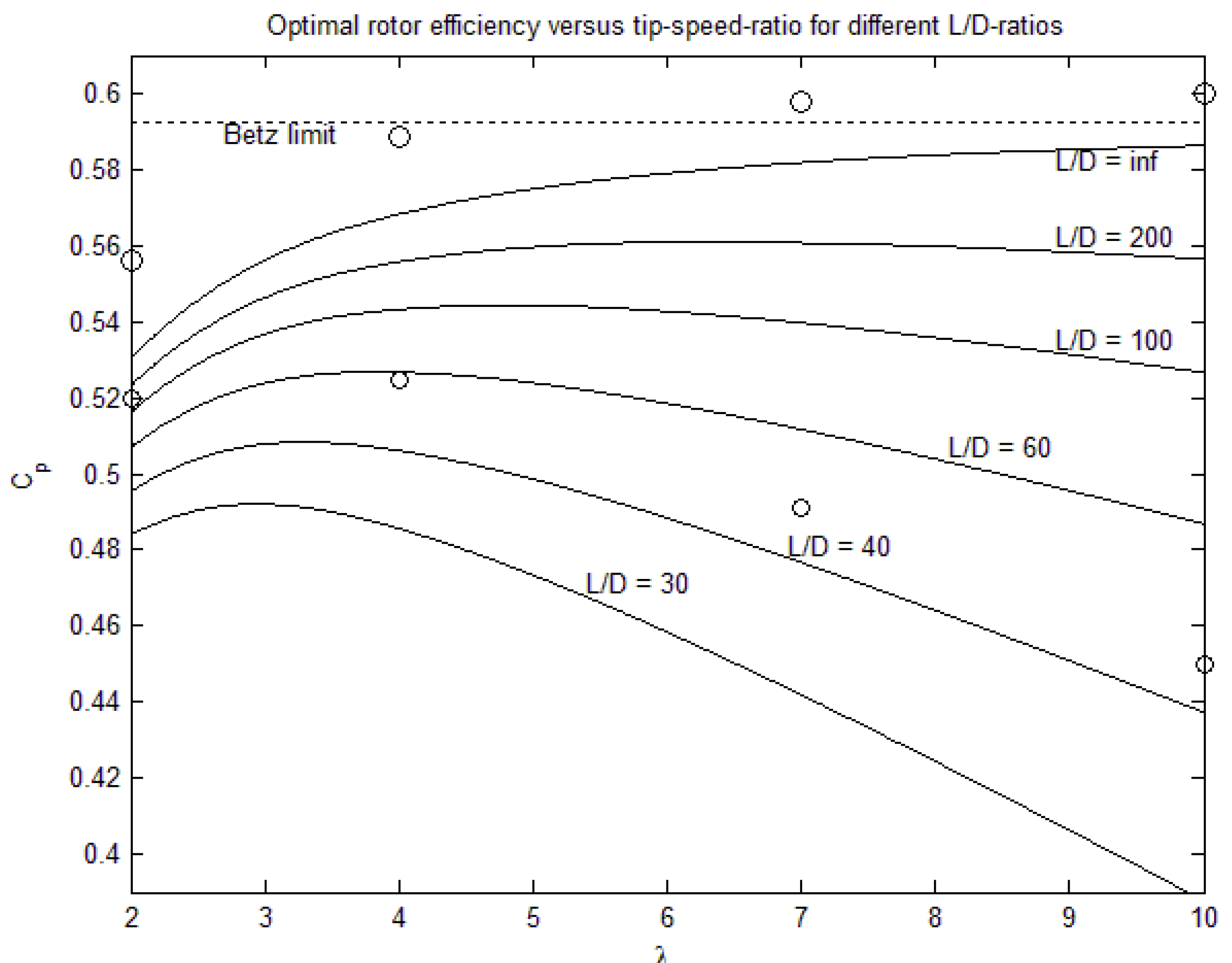
The power-optimal TSR value will depend on viscosity, i.e., the airfoil section L/D ratio. Figure 4 shows this dependency. For a standard L/D = 100 the optimal TSR is seen to be approximately 5. This is lower than the operating TSR of 7 to 10 for large commercial HAWTs. Part of the reason is that tip loss effects are not included in the Figure 4 results. Tip loss effects increase with decreasing TSR, so including tip losses would have shifted the power-optimal TSR to higher values in Figure 4, see e.g., Figure 3.40 in [23].
Regarding tip losses for DAWT rotors, there does not exist any ready-to-use formulation like Prandtl’s model for regular HAWTs. The reason is that in the ideal case of a long diffuser, zero clearance between the truncated tip and the diffuser throat, and a constant bound circulation along the blade, there would be no downwash at the tip and no trailing vorticity. This is comparable to the elimination of trailing vortices in a wind tunnel for airfoil section evaluation, where the tunnel test section is rectangular, and the airfoil section joins the tunnel wall surface perpendicularly in both ends. In reality, the tip-diffuser clearance is finite and depends on manufacturing tolerances as well as allowable aero-elastic deflections of the diffuser. A certain bleed around the truncated tip is inevitable, and will create some degree of downwash. Therefore tip loss effects are present on DAWT rotors, but less pronounced than on regular HAWTs [8,25]. The exact degree to which tip losses are suppressed on DAWTs is highly case-dependent, and beyond the scope of this investigation.
Figure 4.
Optimal rotor averaged power efficiency versus TSR for a range of airfoil glide-numbers computed with the new BEM. No tip losses are included. All the curves are computed with the thrust coefficient value of as BEM input. The four large circular markers are validating HAWT actuator disk (AD) results for infinite L/D. The four small circular markers are HAWT AD results for L/D = 40, see Section 3 for discussion of the BEM-AD comparison.

In the interest of optimizing power, the coupling between TSR and L/D is important and will be briefly discussed here. Again, tip loss effects are left out, since they are less relevant for this investigation. Reducing the design TSR for a wind turbine will cause the blade design to become more bulky. So, how is the operating blade Reynolds number affected, and how will that impact L/D and power efficiency? We can assume that any change in design TSR must be compensated for by adjusting the blade chord along the blade such that the blade’s operating lift capacity is unchanged. The following approximate proportionality relations apply:
which leads to:
The rotor’s operating lift-distribution along the blade can be assumed constant since the rotor-induced blockage will be approximately 1/3. From Equation (22) it then follows that the local airfoil Re and λ are inversely proportional. If the blade designer changes the normal operation λ from value 1 to value 2, then the relative change in design Re is:
Figure 5 is (inevitably) a crude but hopefully representative small compilation of wind tunnel measured maximum L/D for different airfoils relevant to WTGs at varying Reynolds numbers. References are mentioned in the figure legend.
Figure 5.
Measured maximum lift-over-drag ratio versus Reynolds number for selected airfoils relevant for use in Wind Turbine Generator (WTG) rotors, [26,27,28]. The NACA 2415 airfoil is included partly because it has been investigated both at low Re [26] and at high Re [28]. The dotted marker results for NACA 2415 were computed by the airfoil analysis program, XFoil [29]. The two dashed straight lines are linear curve-fits to the XFoil data for low and high Reynolds numbers.
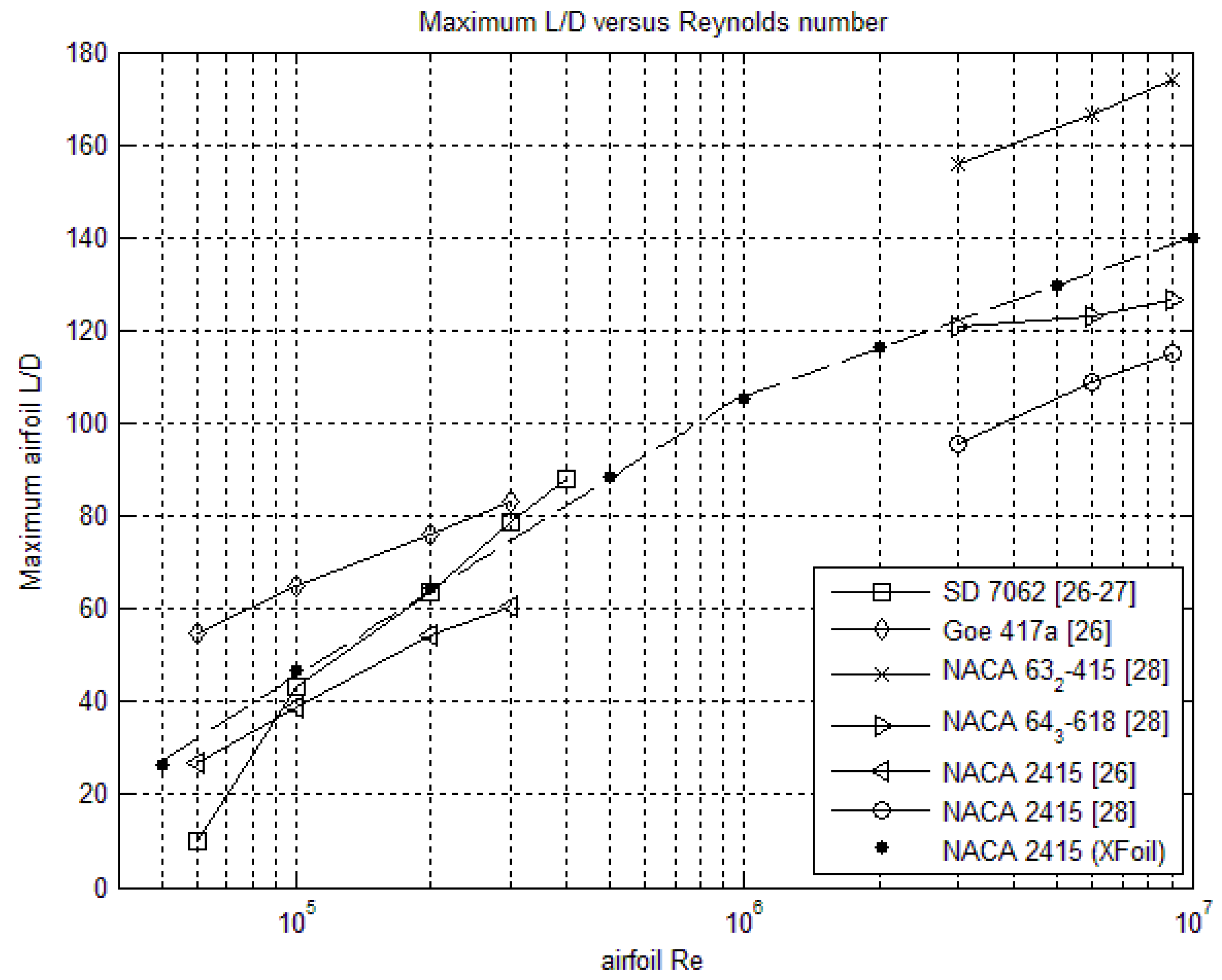
Airfoils are most often designed for a specific application subject to specific requirements, and no single airfoil will excel in all categories, e.g., high L/D, high maximum CL, dirt insensitivity, high thickness, smooth stall, etc. Therefore, attempting to find a general trend between airfoil Re and maximum L/D is a complex task, due to the vast number of differently optimized airfoils and the difficulty of selecting an appropriate group of representative foils among these. With this said, we choose to regard the 2-piece linear fit to the computed NACA 2415 L/D results as indicative for a such general trend.
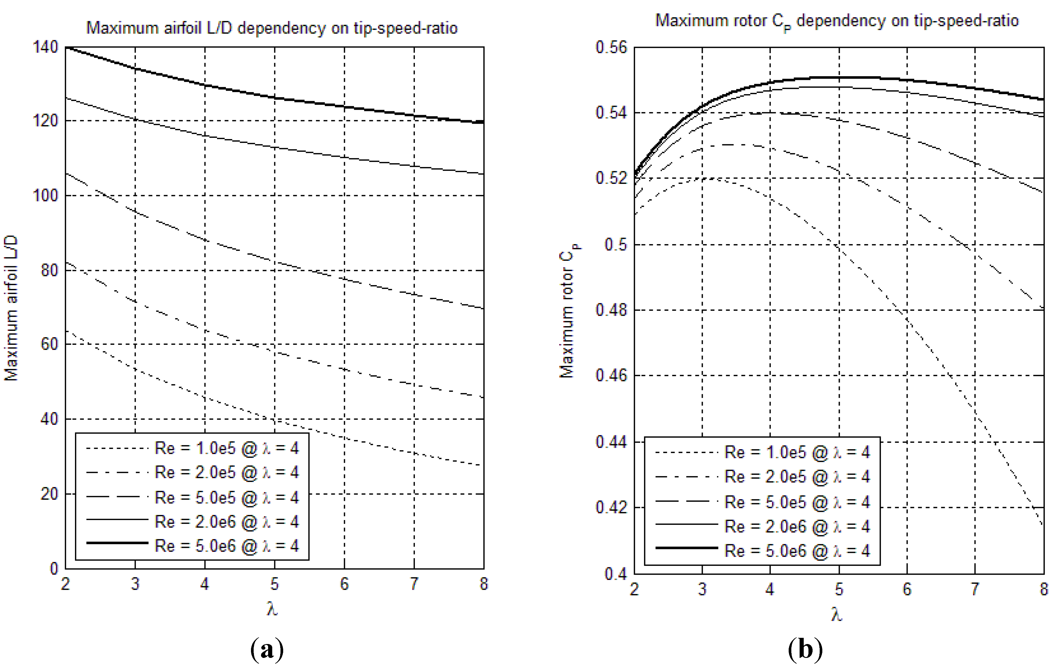
The five curves on Figure 6a show the L/D impact from changing the design TSR, and then adjusting the blade chord distribution accordingly to keep the overall lift capacity constant. These L/D values are then used to compute the maximum rotor power efficiency with the new BEM model. The resulting five curves are displayed in the right subplot. The uppermost curve represents a wind turbine in the MW-range, and the lowermost curve represents a small wind turbine of a few kW rated power. The difference between Figure 4 and Figure 6b is that the former displays “constant L/D” curves whereas the latter displays “constant rotor loading” curves, taking into account the L/D sensitivity to changing TSR, solidity, and Reynolds number, thus providing answer to the posed question from before.
The brief discussion of the TSR’s impact on L/D and subsequent rotor CP ends here. Again, tip losses are not included, so Figure 5 and Figure 6 are most relevant for those turbine types that are less affected by downwash effects at the blade tip. For such turbine types, e.g., DAWTs, a shift to a lower TSR will lead the blade design towards increased operating L/D, which for small WTGs with small blade generally will have a positive impact on maximum rotor CP. The relevance of this will become evident when the AD results are analyzed and discussed in Section 4.
Figure 6.
(a) Impact on L/D when TSR is changed and airfoil Reynolds number is adjusted accordingly using Equation (23) to compensate for the changed lift capacity. The five curves differ by the assumed airfoil Reynolds number at TSR = 4. The curves are computed using the linear curve-fits from Figure 5; (b) The values in the left plot curves have been used as input to the new BEM model to calculate the maximum rotor CP for given values of L/D. The five curves in each subplot are therefore pairwise corresponding.

3. Validation of the Swirled AD Code
The swirled BEM model from Section 2 is a powerful tool. In general, BEM codes are used extensively throughout the wind turbine industry for static and dynamic aero-elastic evaluation of power, loads, stability, control, etc. Over the past several decades BEM add-on features have been developed successfully in order to remedy many of the inherent limitations, e.g., tip loss model, yawed inflow, dynamic inflow, high-load thrust (Glauert correction), dynamic stall, and 3D stall correction. The assumption of tube element independency holds strictly for lightly uniformly loaded rotors with negligible wake expansion and infinite TSR, see Branlard [30]. However, highly loaded rotors, and rotors with expanding wakes due to other mechanisms such as diffusers, will no longer exhibit physical independency between the tube elements. The AD model completely removes the radial element independency assumption. Now the flow field is axisymmetric 2D (with or without swirl) and must be solved using CFD. The rotor disk becomes a thin plate sub-domain in which external forces from the rotor on the fluid can be applied in axial and tangential direction. For details, see, e.g., Mikkelsen [31] or Hansen [21].
3.1. AD Model
In this investigation, the AD code was developed using a commercial Navier-Stokes solver by Comsol MultiPhysics® [32]. The governing equations are the viscous, incompressible Reynolds-averaged Navier-Stokes (RANS) equations in axisymmetric coordinates, which are discretized using a weak form Galerkin finite element formulation. The finite element basis functions are linear (P1P1). Discretization independence tests with higher order quadratic (P2P1) and cubic (P3P2) basis functions were performed and results are presented in Table 2. The PxPy naming convention is used by Comsol. P1 stands for a 1st order (linear) polynomial basis, P2 stands for a 2nd order polynomial basis, etc. Due to numerical stability, the order of the pressure polynomial decomposition is one lower than for the remaining variables, e.g., P3P2, except for 1st order elements (P1P1) where 1st order accuracy is used for all variables. Segregated Newton solvers are used for the primitive variables and the turbulence variables. The projection method [33] used for the incompressible RANS employs consistent streamline and crosswind diffusion for numerical stability and pseudo-timestepping for advancing the temporal marching towards a steady solution. The applied turbulence model is the standard κ – ε formulation, where κ is the turbulent kinetic energy, and ε is the dissipation rate of turbulent energy. The wall function used by Comsol for proper modeling of the innermost part of the turbulent boundary layer requires ideally a boundary mesh first layer height of y+ = 11.06 or below, which corresponds to the distance from the wall where the logarithmic boundary layer meets the viscous sublayer [32]. The off-range y+ impact on extracted power, flow separation, etc. is listed in Table 2.
Mesh/discretization independency test results are shown in Table 2 for the Hansen and the multi-element DAWT configurations at power-optimal thrust loading. These configurations are explained in detail in Section 4. The discretization setup used for all subsequent computations are marked with bold, i.e., P1P1 polynomial basis, boundary layer 1st element height of 0.01 mm for the Hansen diffuser, and 0.005 mm for the multi-element diffuser. The first three mesh independency test runs are for increasing the polynomial basis to higher order accuracy. The power efficiency coefficient, CP, drops from 0.9054 by less than 0.4% when switching to higher order shape functions. The y+ is in the recommended range. P1P1 is favored because of higher execution speed. It does require more mesh elements than would be needed with, e.g., P2P1 or P3P2, but this is rather convenient for obtaining high geometric resolution of the diffusers, not least for the multi-element diffuser. In the next four runs of Table 2 the first layer element height, δw, is reduced from coarse to very fine. A δw of 0.01 mm leads to recommended values for y+. Increasing or decreasing δw by one order of magnitude has a limited impact on CP of only 0.1%. The last four runs of Table 2 are similar to the four previous, but with the multi-element diffuser instead of the Hansen diffuser. Deviations from the optimal δw = 0.005 mm by one order of magnitude leads to minor CP changes of 0.7%. The impact on flow separation location on the most downstream vane 8 in layer 1 (see next section’s Figure 11b) is shown in the last column.
| Configuration | Poly. Basis | [–] | [–] | [mm] | [–] | Avg() [–] | Max() [–] | Sep.loc. [%] |
|---|---|---|---|---|---|---|---|---|
| Hansen DAWT, case1 | P1P1 | 0.77 | 10 | 0.01 | 0.9054 | 4.05 | 10.2 | 100 |
| Test: Increasing polynomial | P2P1 | 0.77 | 10 | 0.01 | 0.9021 | 4.11 | 11.3 | 100 |
| basis order. | P3P2 | 0.77 | 10 | 0.01 | 0.9018 | 4.12 | 12.7 | 100 |
| Hansen DAWT, case1 | P1P1 | 0.77 | 10 | 1 | 0.9195 | 347 | 856 | 100 |
| Test: Decreasing 1st elm. | P1P1 | 0.77 | 10 | 0.1 | 0.9043 | 40.5 | 64.7 | 100 |
| height in boundary layer, | P1P1 | 0.77 | 10 | 0.01 | 0.9054 | 4.05 | 10.2 | 100 |
| P1P1 | 0.77 | 10 | 0.001 | 0.9061 | 0.40 | 1.12 | 100 | |
| Multi-element DAWT, case1 | P1P1 | 1.07 | 2 | 0.5 | 1.6431 | 358 | 620 | 54 |
| Test: Decreasing 1st elm. | P1P1 | 1.07 | 2 | 0.05 | 1.6491 | 36.5 | 55.9 | 80 |
| height in boundary layer, | P1P1 | 1.07 | 2 | 0.005 | 1.6372 | 2.23 | 8.79 | 81 |
| P1P1 | 1.07 | 2 | 0.0005 | 1.6259 | 0.40 | 0.97 | 77 |
The governing NS equations constitute an almost exact representation of the real physics. Still, model approximations are introduced through the use of a turbulence model, the axisymmetric assumption, and discretization errors. The disadvantage of RANS CFD is the computational execution time. A converged solution for an axisymmetric 2D domain with 0.3–0.5 million mesh elements is obtained after 150–200 pseudo-timesteps in approximately 1 hour on a multi-core desktop pc. Configurations with low disk-loading converged perfectly with residual reductions by five or more orders of magnitude. Convergence for higher loaded configurations near peak power would often level off after 3–4 orders of magnitude residual reduction. Configurations with heavily loaded disks and stalled wake flows would see residual reductions of only 2–3 orders of magnitude, and sometimes exhibit transient instabilities. In these cases representative (average) values for the extracted power would be used. A few high-load configurations at post-peak conditions were so unstable that no power results were calculated.
The 2D axisymmetric domain for the AD CFD validation test cases corresponds to a bare propeller HAWT, see Figure 7. The domain extends 100 R upstream and downstream of the disk and on average 96 R in the radial direction. The Reynolds number based on the rotor (disk) radius R and free stream velocity is 4.7e6. This is equivalent to a 7.2 m rotor radius at a free stream velocity of 10 m/s. The disk thickness is 0.04 R. The domain inlet is on the lower boundary of the domain, and the axisymmetric axis on the left domain boundary. Remaining domain boundaries are outlets with a zero pressure gradient Neumann condition. The specified inlet turbulence intensity is 5% with a length scale of 0.02 R. These disk, domain, and flow specifications are kept constant throughout the investigation unless otherwise noted.
The mesh for the validation test cases is hybrid block-structured/unstructured. The four structured blocks are the disk sub-domain, the wake behind the disk, plus two more blocks next to the first two in domain radial direction. The purpose of the structured mesh is to capture the wake with as little numerical diffusion as possible, see Figure 7, in order to exclude that as a source of error regarding eventual discrepancy between BEM and AD results. The remaining mesh is unstructured. The entire mesh consists of 418377 elements of which 306000 are structured quadrilaterals. The disk subdomain on which the axial and azimuthal volume forces are applied counts 2000 elements (20 × 100).
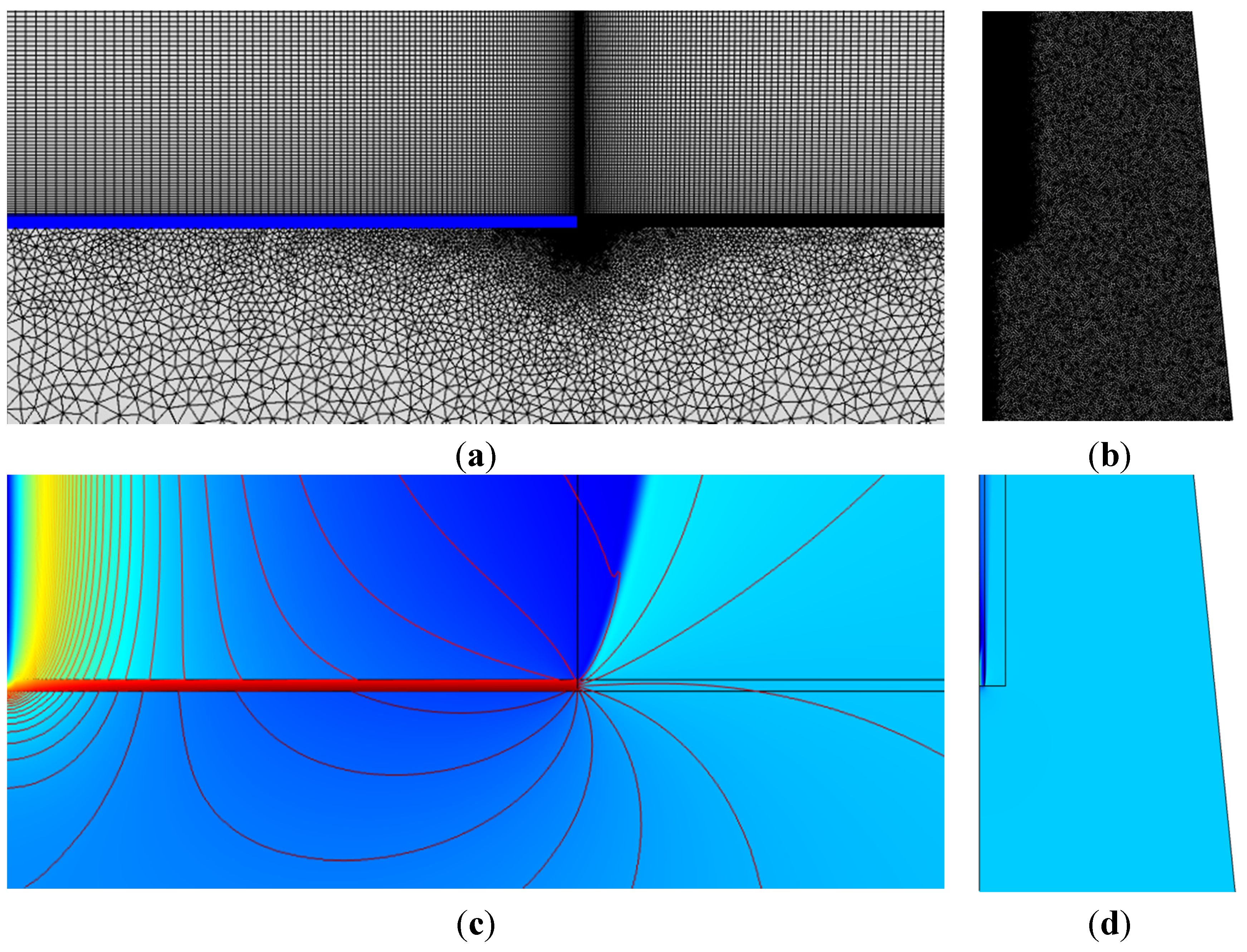
Figure 7.
Domain mesh (a,b) and example of domain solution with pressure contour lines and axial velocity surface colors (c,d). (a,c) Disk sub-domain zoom-ins.
Figure 7.
Domain mesh (a,b) and example of domain solution with pressure contour lines and axial velocity surface colors (c,d). (a,c) Disk sub-domain zoom-ins.

The external disk forces are applied exactly as the BEM forces. Infinite L/D is assumed initially, so all forcing from the disk on the fluid will be directed perpendicular to the local flow through the disk, as depicted in Figure 2a. The disk represents straight rotating blades perpendicular to the center-axis, and do not exert any radial forcing. The external forcing is specified as a force-per-volume is each direction, and in accordance with the specified BEM forcing in Equation (5) from Section 2. Axial, tangential, and radial forcing components are:
Where u and w are the local axial and tangential velocity components.
The thrust and power coefficients are computed locally on each cell of the disk sub-domain and integrated over the disk volume. Note the exact similarity with the BEM Equations (16)–(19).
and are the rotor-averaged power efficiencies delivered by the disk lift forces and drag forces respectively. In the ideal case of no viscous drag will vanish, and CP can then alternatively be expressed as the sum of power efficiencies resulting from the axial and azimuthal forcing:
3.2. AD Results
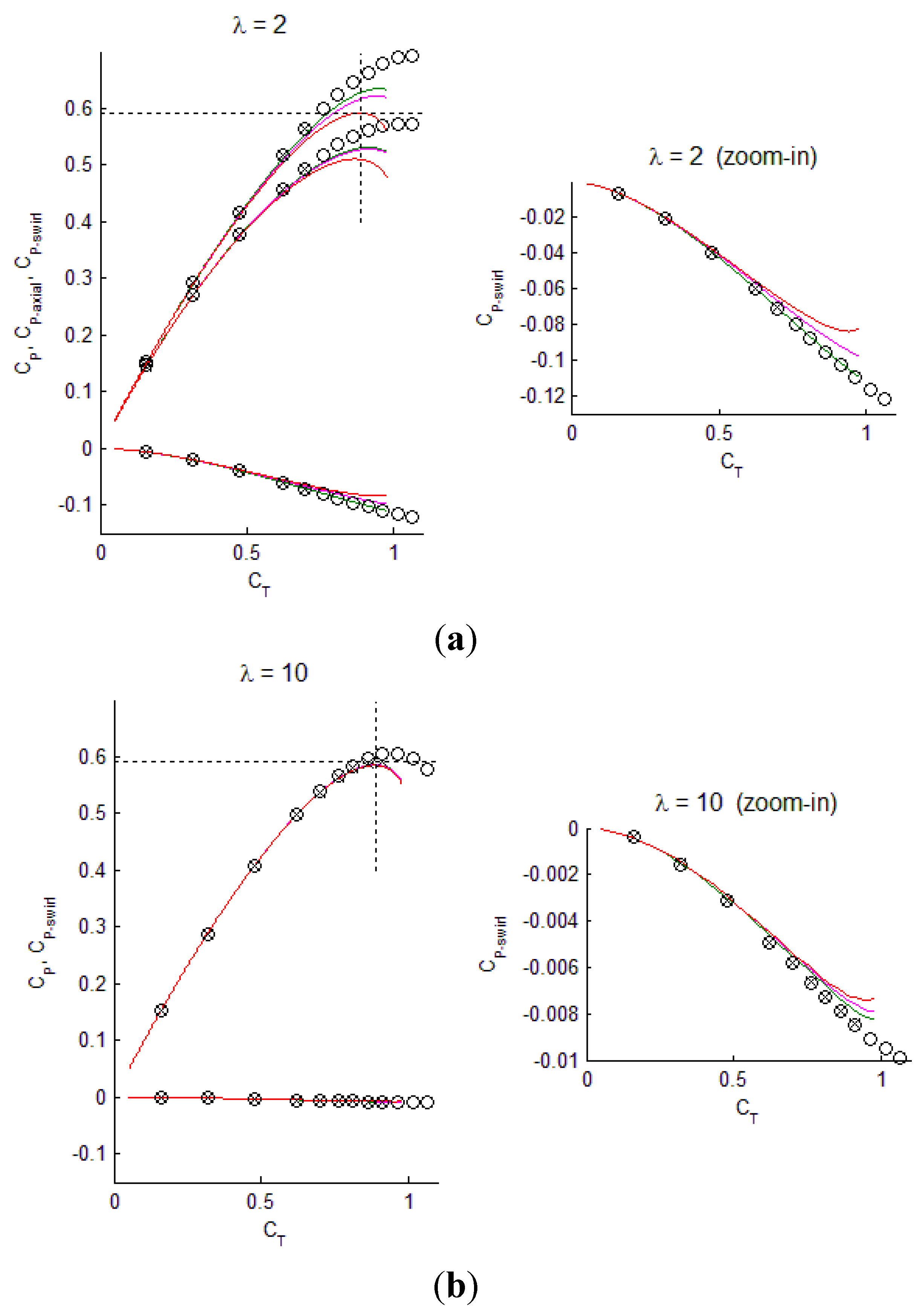
The rotor-averaged , , and total CP for the 36 converged AD solutions are displayed on Figure 8. The following conventions apply: Red lines are results using the standard BEM model with no far wake pressure loss term. The purple lines are for the BEM model with Burton’s [23] simplified pressure loss term, and the green lines are for the present BEM model with full inclusion of the far wake pressure loss.
The circle markers are AD CFD results with RANS as the governing equations (). The cross markers are AD results with the inviscid NS as the governing equations. The black dotted lines mark the Betz limit of at for an infinite TSR rotor. We observe that the inviscid NS and RANS AD results are nearly identical, and that the action of domain flow viscosity has negligible impact on the AD performance at low and medium rotor loading below peak power. At peak power the AD results for the high TSR of 10 indicate that the slightly higher CP obtained with the RANS AD model compared to both the NS AD model and the BEM model partly stems from favorable flow mixing between the turbulent viscous wake and the surrounding flow. The observable discrepancy between AD results and BEM results can therefore be attributed to 1) the absence of wake turbulence in the BEM, and 2) high-loading effects such as increased radial flow in the vicinity of the disk and wake expansion, which invalidate the tube-element independency assumption of the BEM methods. The high-loading effects seem to “kick in” at lower thrust loading for the low TSR of 2. High load BEM model inadequacy was observed long ago by Glauert and motivated his correction for highly loaded rotors [34]. At lower loadings, the BEM assumptions are not violated, and excellent agreement with the AD results are seen, both for the axial and azimuthal power contributions. The present BEM method with full wake pressure loss inclusion (green) shows the best fit with the AD results, but also the BEM with simplified pressure loss term (purple) performs very well. The onset of high loading effects lead to slightly higher performance for the AD model compared to BEM.
Figure 8.
BEM and AD rotor-averaged HAWT power-performance comparison for low TSR (a) and high TSR (b) versus thrust coefficient, CT.
Figure 8.
BEM and AD rotor-averaged HAWT power-performance comparison for low TSR (a) and high TSR (b) versus thrust coefficient, CT.
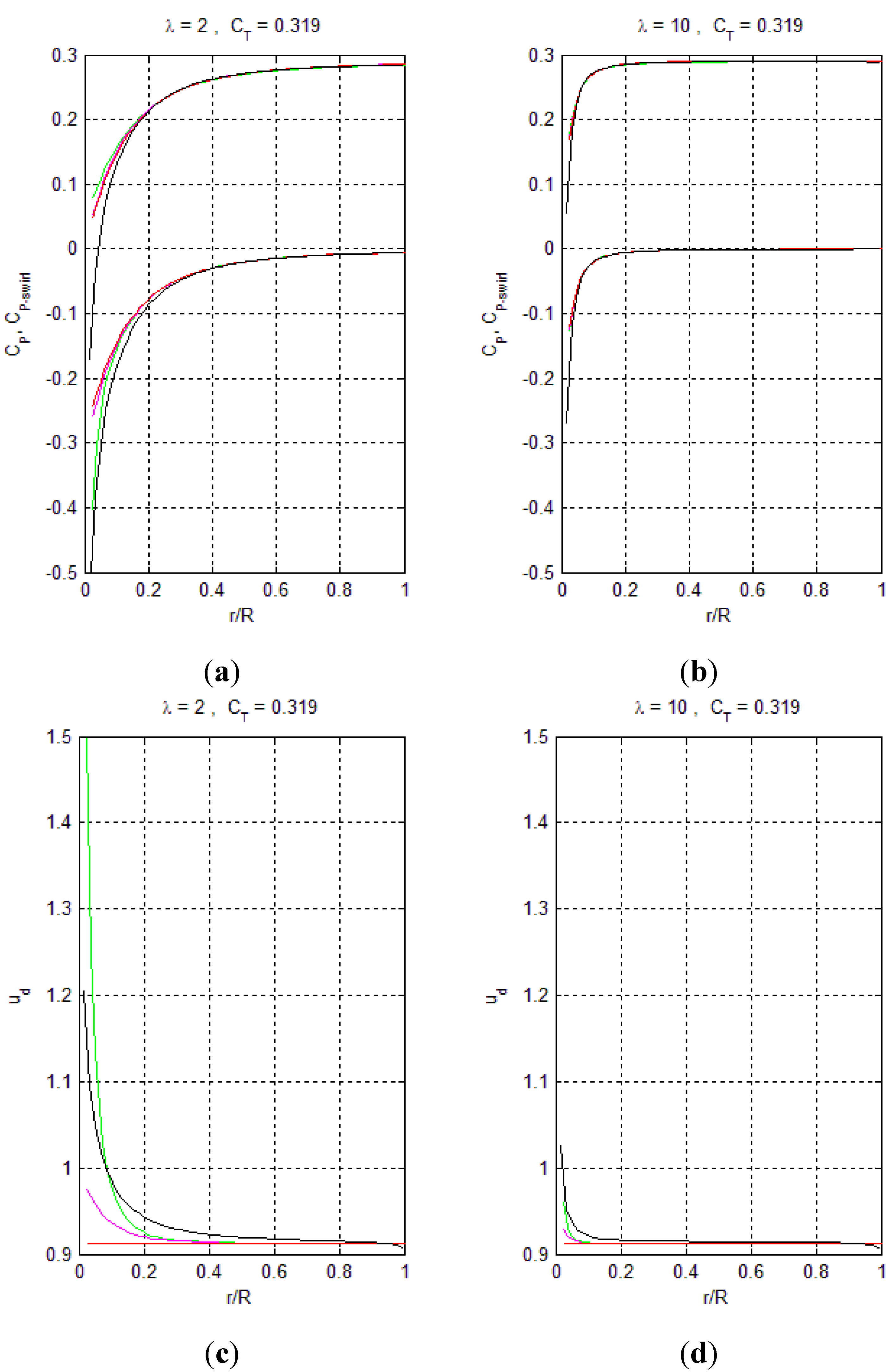
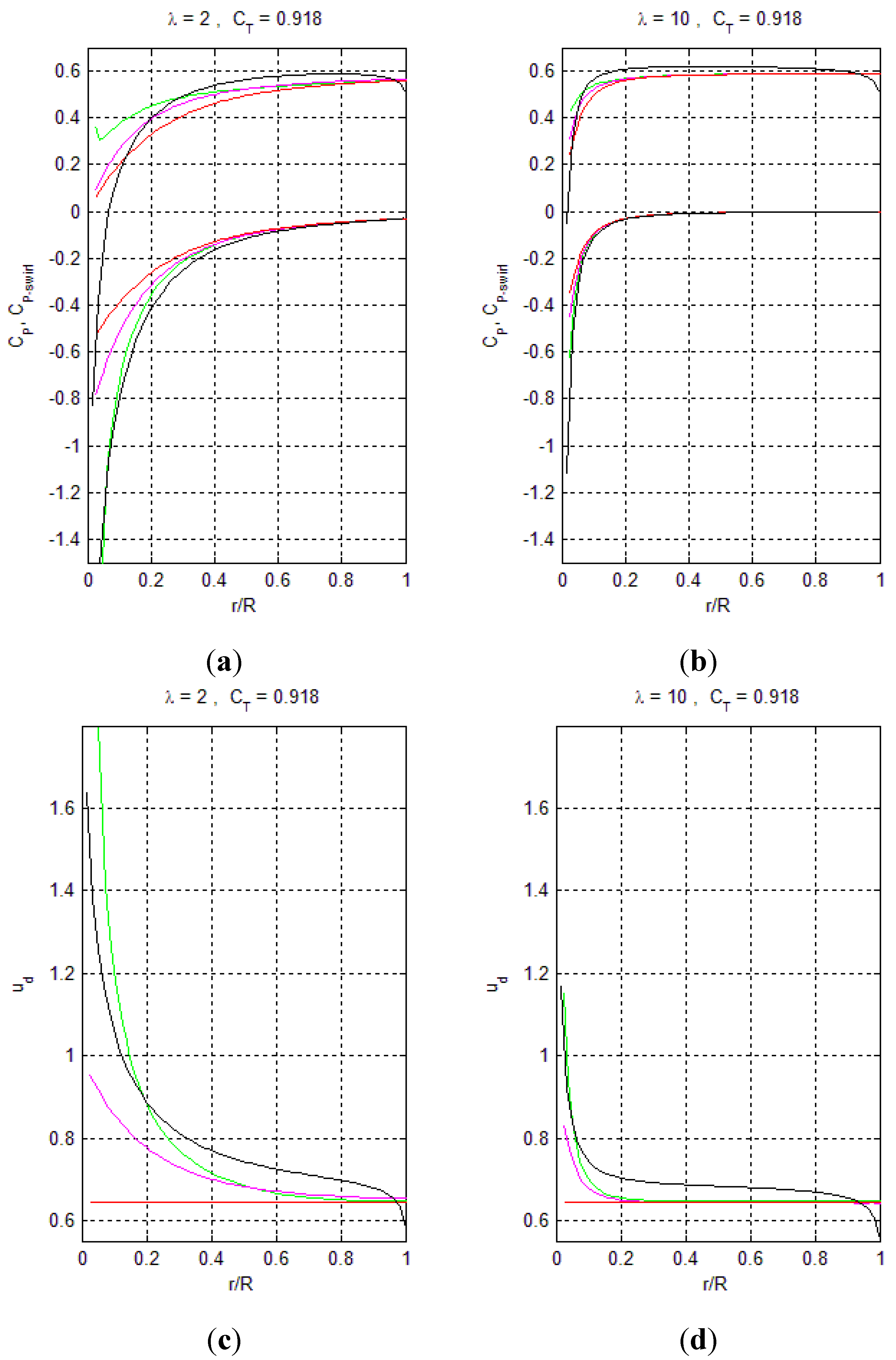
On Figure 9 and Figure 10 are shown the spanwise distributions for local power coefficients and normalized axial flow velocity through the rotor disk. The BEM color conventions from Figure 8 and Figure 3 apply. The black curves are the AD results. One can observe that for high TSR = 10 and low uniform thrust loading (Figure 9b) the agreement between BEM and AD is excellent, as expected. But even so, differences in mass-flow distributions through the rotor (Figure 9d) are noticed. Standard BEM (red) predicts uniform mass-flow, whereas the present BEM with full wake pressure loss captures the swirl-induced mass-flow augmentation through the inner part of the disk. The AD curve shows a flow-rate decrease at the tip, presumably due to radial deflection of the expanding streamlines, which is not captured by any BEM method. These findings agree qualitatively well with the AD-BEM comparison by Madsen et al. [22]. At low uniform thrust and low TSR = 2, Figure 9a,c shows similar but increased trends for center flow augmentation and mass-flow decrease at the tip. Figure 10 resembles Figure 9 but with high uniform loading, , approximately corresponding to the peak power operational condition. The standard BEM center mass-flow prediction at low TSR = 2 is significantly under-predicted, whereas the present BEM agrees much better with the AD curve.
Figure 9.
BEM (colored) and AD (black) spanwise distribution of power (upper) and mass-flow (lower) at low thrust loading, for a regular HAWT. (a,c) TSR = 2; (b,d) TSR = 10.
Figure 9.
BEM (colored) and AD (black) spanwise distribution of power (upper) and mass-flow (lower) at low thrust loading, for a regular HAWT. (a,c) TSR = 2; (b,d) TSR = 10.

The general trend for the AD model to predict higher mass-flow over a broad range spanning the mid part of the “disk blades” is not captured by any BEM method, and hence attributable to the streamline deflection and wake expansion.
Figure 10.
BEM (colored) and AD (black) spanwise distribution of power (upper) and mass-flow (lower) at high thrust loading, for a regular HAWT. (a,c) TSR = 2; (b,d) TSR = 10.
Figure 10.
BEM (colored) and AD (black) spanwise distribution of power (upper) and mass-flow (lower) at high thrust loading, for a regular HAWT. (a,c) TSR = 2; (b,d) TSR = 10.
Concerning the influence of drag, four AD RANS CFD runs were made with a finite , and TSR values 2, 4, 7, 10, and four other runs were made with infinite L/D and the same TSR values.
The disk loading for all eight runs was constant at the power-optimal ideal value of . Power performance for these eight runs is plotted in Figure 4 and can be compared directly with the corresponding BEM-based curves for infinite L/D and The results are very consistent with the CP results of Figure 8 at , where the present BEM method seems to under-predict the optimal CP by 0.03 at low TSR = 2, and by 0.01 at high TSR = 10.
In summary, the swirled AD model is in excellent agreement with the present BEM method for operational conditions where the BEM tube element independency assumption is generally valid, i.e., at low thrust loading. The validated swirled AD model will be the work horse for developing proper rotor design guidelines for DAWTs in the next section.
4. DAWT Rotor Design
Conceptually, the flow through a DAWT is comparable to a swirled flow through an expanding nozzle for which reference results already exist. Clausen and Wood [35] identified a recirculation criterion for swirled nozzle flows based on the normalized swirl velocity and an expression for the critical expansion ratio, valid for “solid body” rotating flows. In the experimental work of [36], Clausen et al. described the tendency of swirl to suppress recirculation on the diffuser (nozzle) surface, while at the same time causing premature vortex breakdown of the core flow. The swirled flow through a diffuser DAWT has increasing rotational velocity towards the core, and not “solid body” rotation. Furthermore the presence of a pressure drop across the disk causes a natural tendency of the pressure to recover and the wake to expand, not found in classical swirled nozzle flows. However, the two types of flows share similarities, and the described inner core stall and diffuser wall stall scenarios can obviously occur for DAWT flows also. The exact role of swirl and the disk interaction is of particular interest here. Swirl rate is primarily controlled through rotor TSR and axial disk interaction primarily through rotor thrust distribution.
4.1. Configurations
Three WTG configurations are investigated, see Figure 11:
The regular HAWT is the baseline against which we compare power performance, resistance to stall, etc. The Hansen DAWT represents the classical single-element low-expansion and rather long type of diffuser, and is well described in literature. The multi-element DAWT is the newly developed high-expansion and very compact diffuser. For each of these WTG configurations, four nacelle/rotor solutions are investigated, see Figure 12:
- Case 1: Full disk, uniform loading.
- Case 2: Disk with centerhole, uniform loading.
- Case 3: Disk with centerbody, uniform loading.
- Case 4: Disk with centerbody, uniform loading with inner ramp-down.
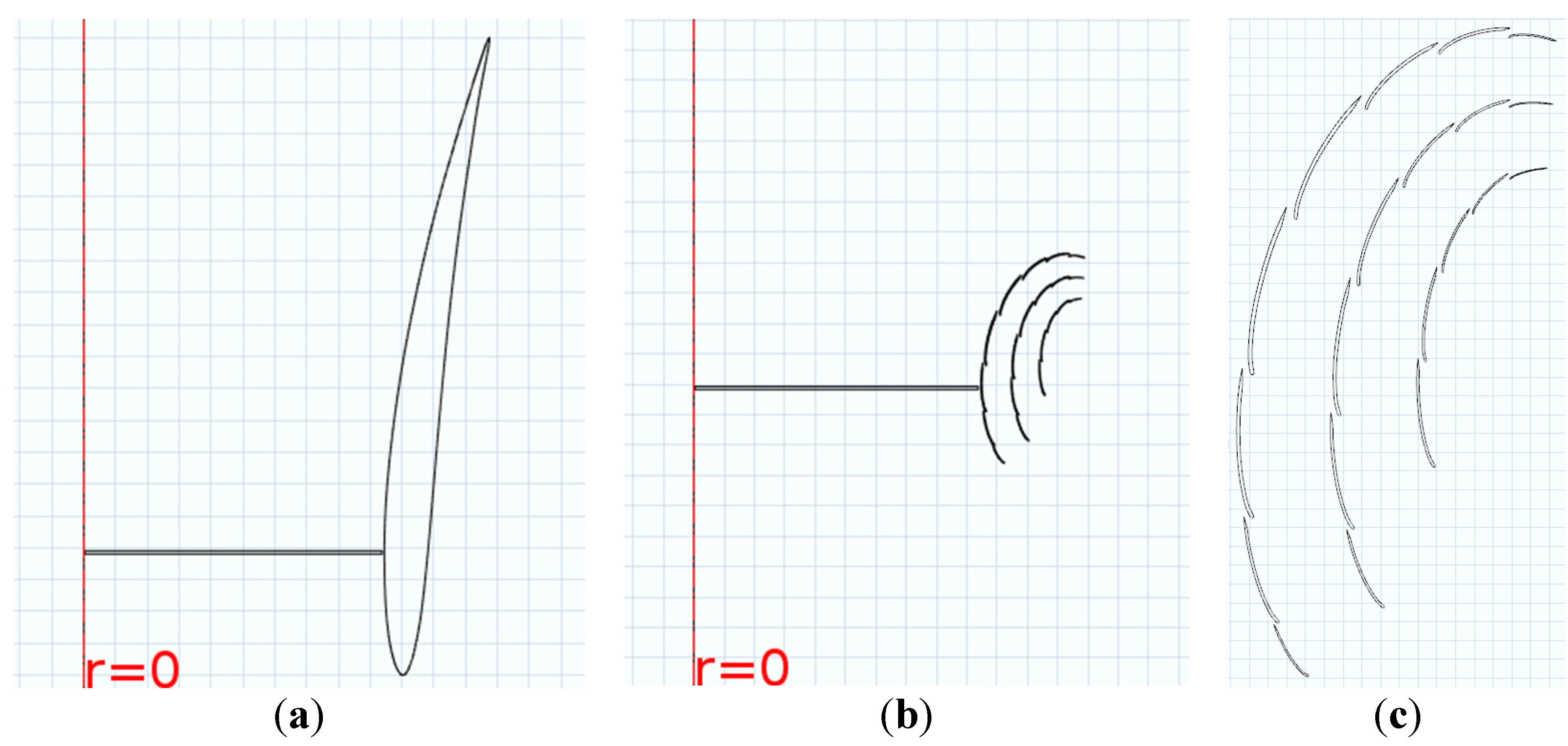
Figure 11.
The two diffuser configurations: (a) Hansen diffuser; (b) Multi-element diffuser. The frontal areas are comparable: and for the Hansen and multi-element diffuser respectively. Lengthwise, the corresponding numbers are: and , the latter being significantly more compact. (c) Zoom of multi-element diffuser.

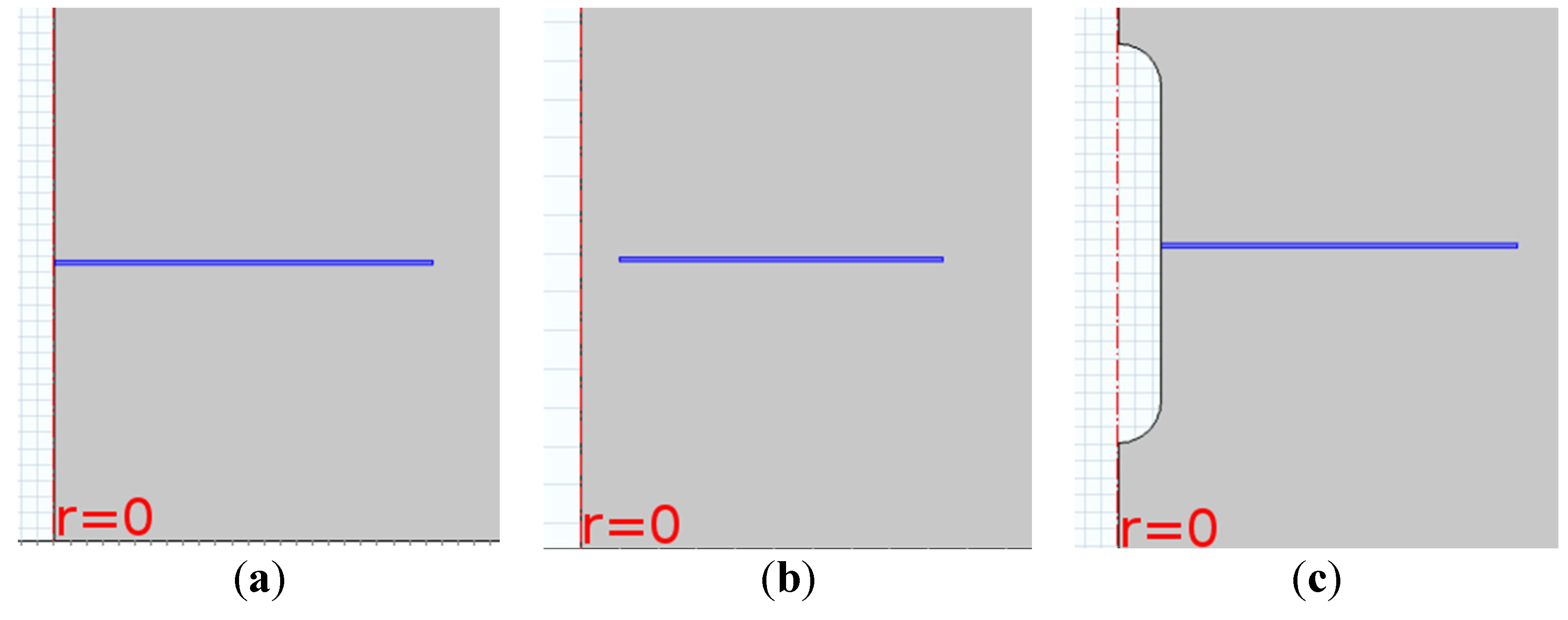
Figure 12.
Nacelle/rotor configurations: (a) Case 1 full disk; (b) Case 2 disk with center-hole; (c) Cases? 3–4 disk with centerbody.
Figure 12.
Nacelle/rotor configurations: (a) Case 1 full disk; (b) Case 2 disk with center-hole; (c) Cases? 3–4 disk with centerbody.

The cases 1–4 are chosen to observe at what point inner core vortex breakdown becomes critical during the nacelle “transition” from the ideal case 1 to the realistic cases 3 and 4, the latter used for exploring possible ways to avoid eventual core stall tendencies at premature thrust loading. Note that “vortex breakdown” and “core stall” are both loosely defined to cover any occurrence of reversed axial flow velocity in the inner part of the wake. For each of cases 1–4 a high-swirl and a low swirl rotor is investigated:
- High swirl: TSR = 2
- Low swirl: TSR = 10
The high swirl slowly rotating rotor blades will have a high solidity approaching unity on the inner part not unlike a nozzled propeller for a vessel. Contrarily, the low swirl fast spinning rotor blades will be slender as known from large wind HAWTs. For each combination of WTG, nacelle/rotor, and TSR 14 different levels of axial disk forcing (thrust) are analyzed ranging from to . In total 336 actuator disk RANS CFD runs.
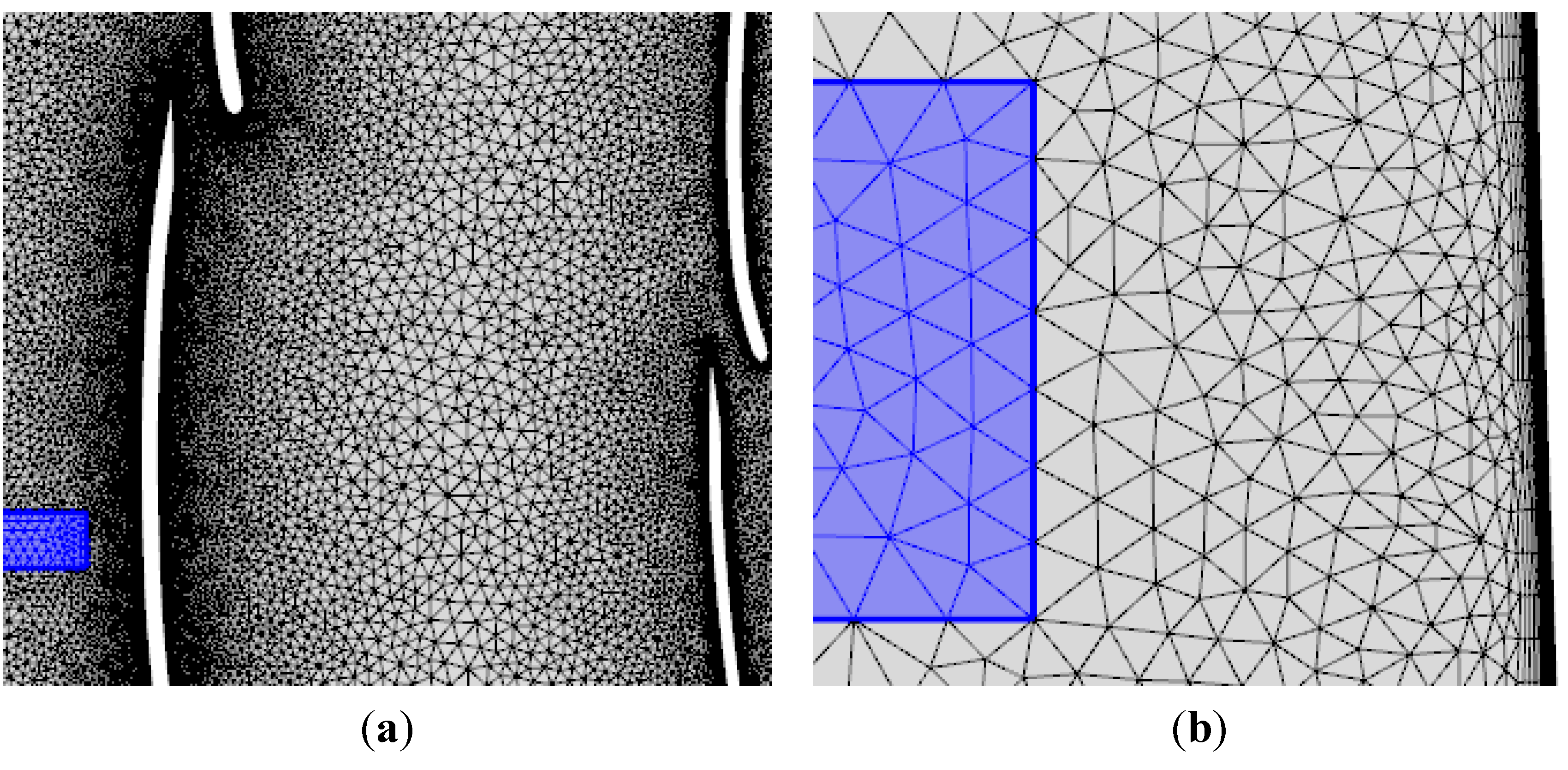
Due to the diffuser geometries, unstructured meshing is used for these AD runs, except on all wall surfaces on diffusers and center-bodies where 20 to 32 layers of anisotropic structured boundary layer elements are applied with a normal stretching ratio of 1.15. Mesh details for the multi-element DAWT rotor tip vicinity are shown on Figure 13. The disk thickness is 0.01 R. The total element counts are approximately 120000, 320000, and 460000 for the HAWT, the Hansen DAWT, and the multi-element DAWT respectively. The same sizing parameters are used for all meshes. In general the domain discretization is very sufficient, and a high degree of mesh independency is achieved, see Table 2 from the previous section.
Figure 13.
(a) Mesh zoom-in; (b) Zoom-in of left zoom-in. The blue subdomain is the AD tip.
The external disk forces for the centerbody configuration with uneven axial loading (nacelle/rotor case 4) will be explained. Instead of assuming an ideal blade root with negligible drag and full lift capacity to deliver the loading all the way inboard towards the hub (centerbody), we choose a more conventional inner blade design with a gradual transition from ideal aerodynamic profiles to the circular cylinder at the blade root flange. The transition starts at and ends at the centerbody radius at . Over this radial transition range there is a linear ramp-down of ideal airfoil lift-forces from 100% to 0%, and a simultaneous ramp-up of circular cylinder drag forces from 0% to 100% at the root. The formulation of volume disk forces in the AD model for nacelle/rotor case 4 is similar to Equations (27)–(30) which apply to nacelle/rotor cases 1–3, but modified on the inner transition part of the rotor:
where and are the weight factors of the cylinder drag forcing and the airfoil lift forcing respectively.
The azimuthally disk-averaged axial forcing per volume from the cylinder (or transitional) inboard part of the blades is:
Similar for the tangential forcing:
where W is the magnitude of the tangential and axial wind components in the rotating blades’ reference.
The disk is assumed to consist of three blades, , the circular cylinder drag coefficient, , and the cylinder root chord is normalized with the blade tip radius, . The thick cylinder chord is reasonable for small wind household turbines for which this investigation will turn out to be most relevant. For large wind turbine would be smaller, approximately 0.05.
4.2. DAWT Results
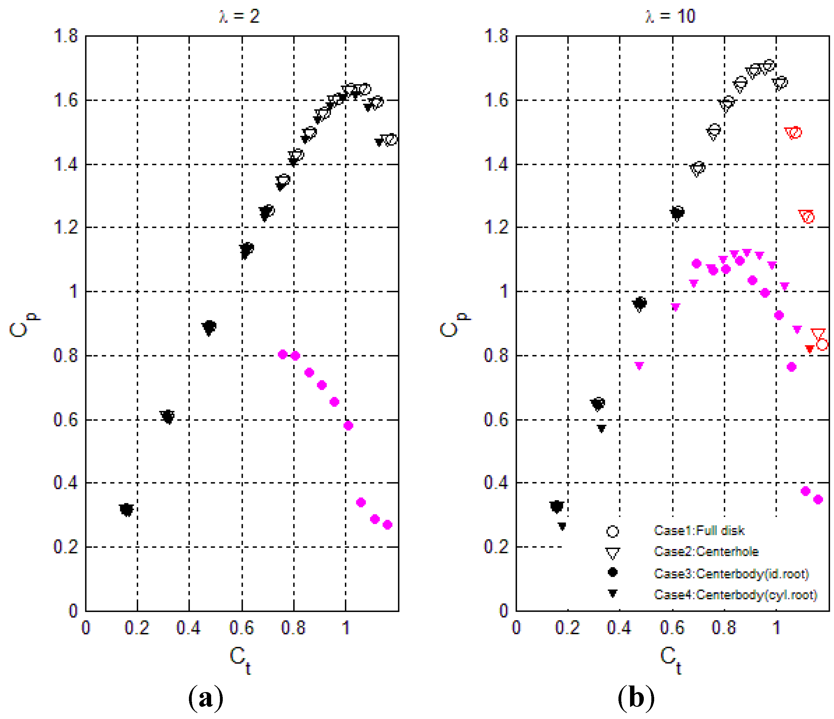
The power performance of all AD runs will be presented and discussed in the following. Color coding will be used on the plots to indicate the eventual type of stall encountered in the flow:
- Black: No stall
- Red: Inner wake stall (vortex breakdown)
- Purple: Centerbody surface stall
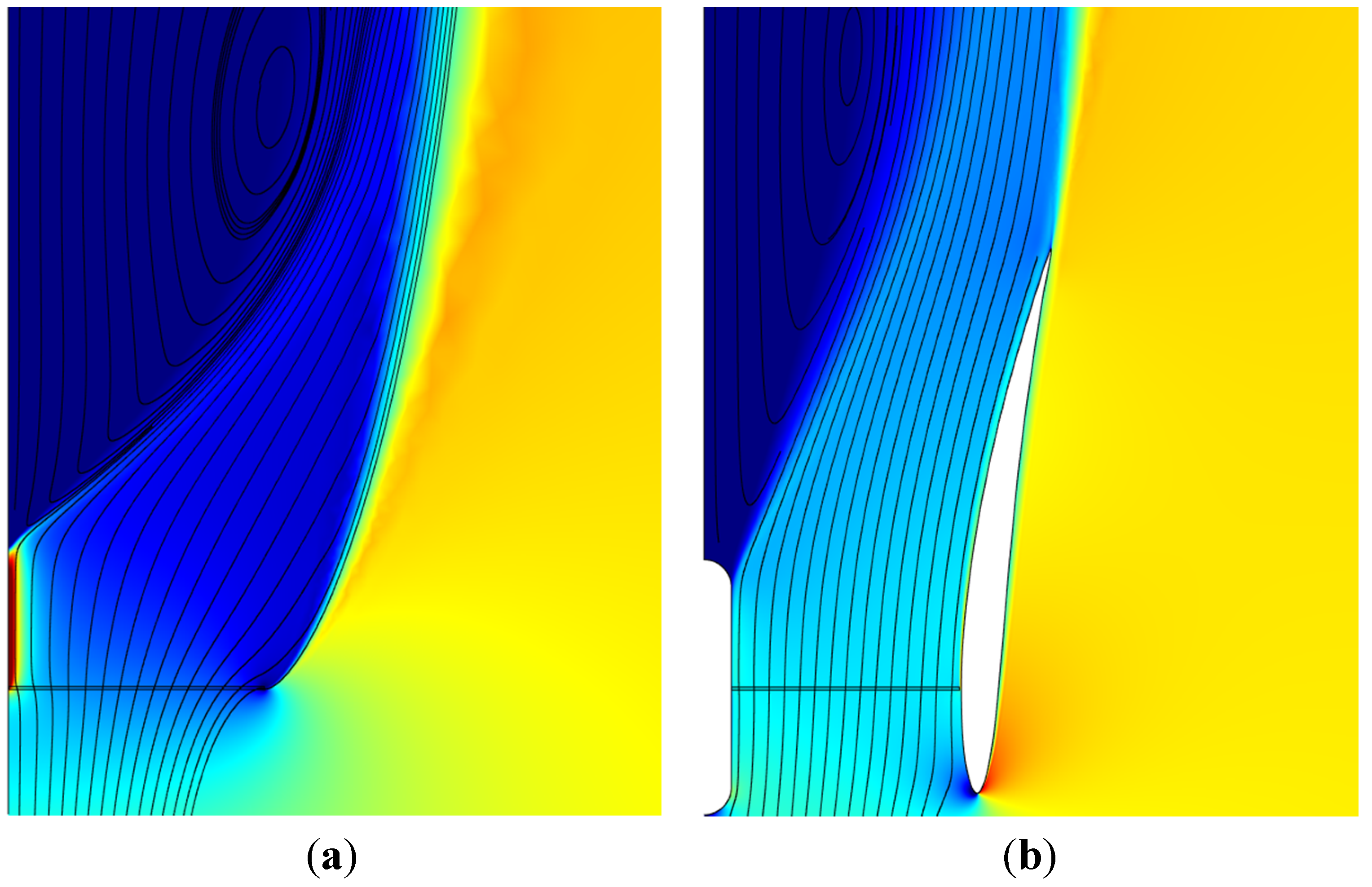
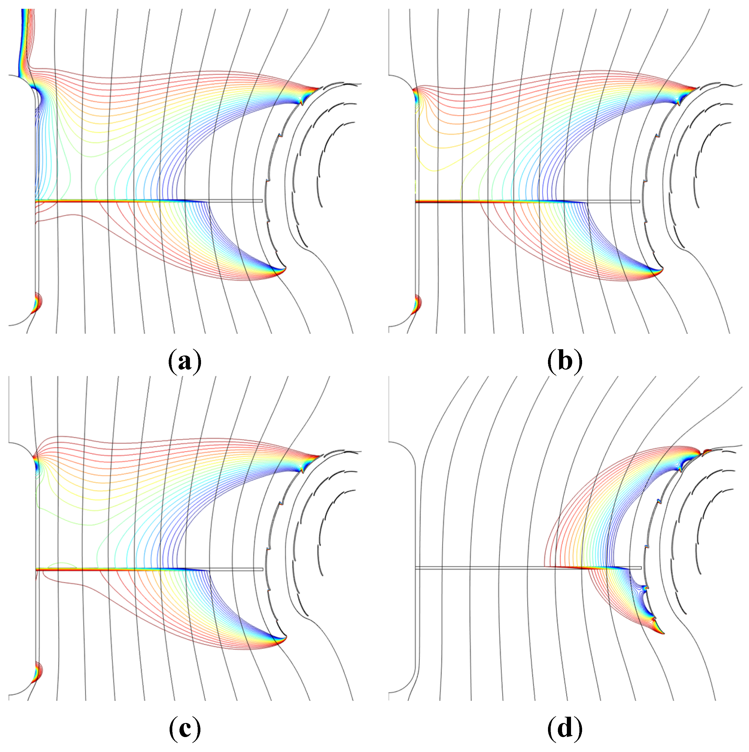
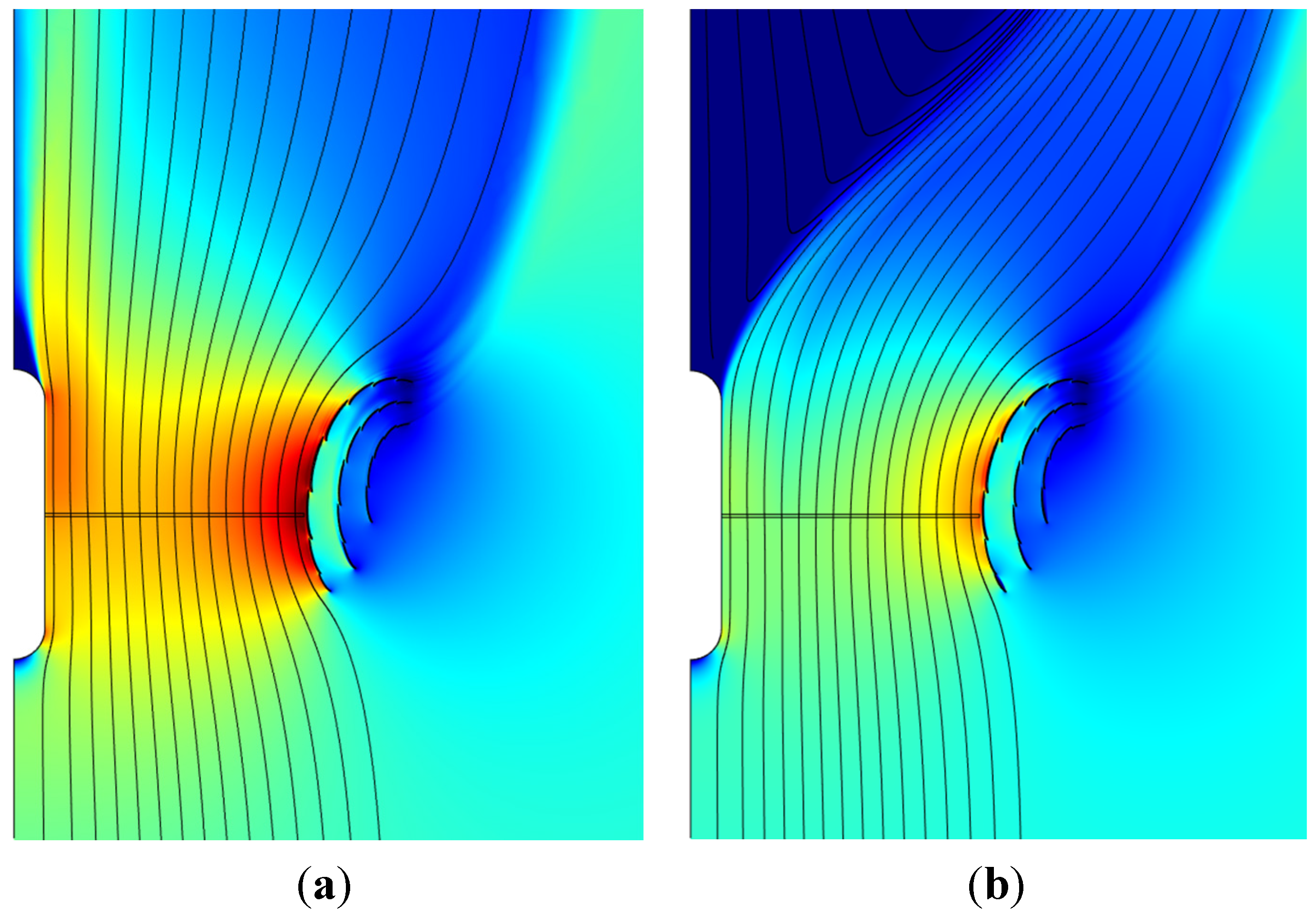
Examples of the two stall types are shown in Figure 14. The streamlines through the disk are black, and the surface colors visualize the axial flow velocity. The same color range is used on Figure 16, Figure 18, and Figure 20.
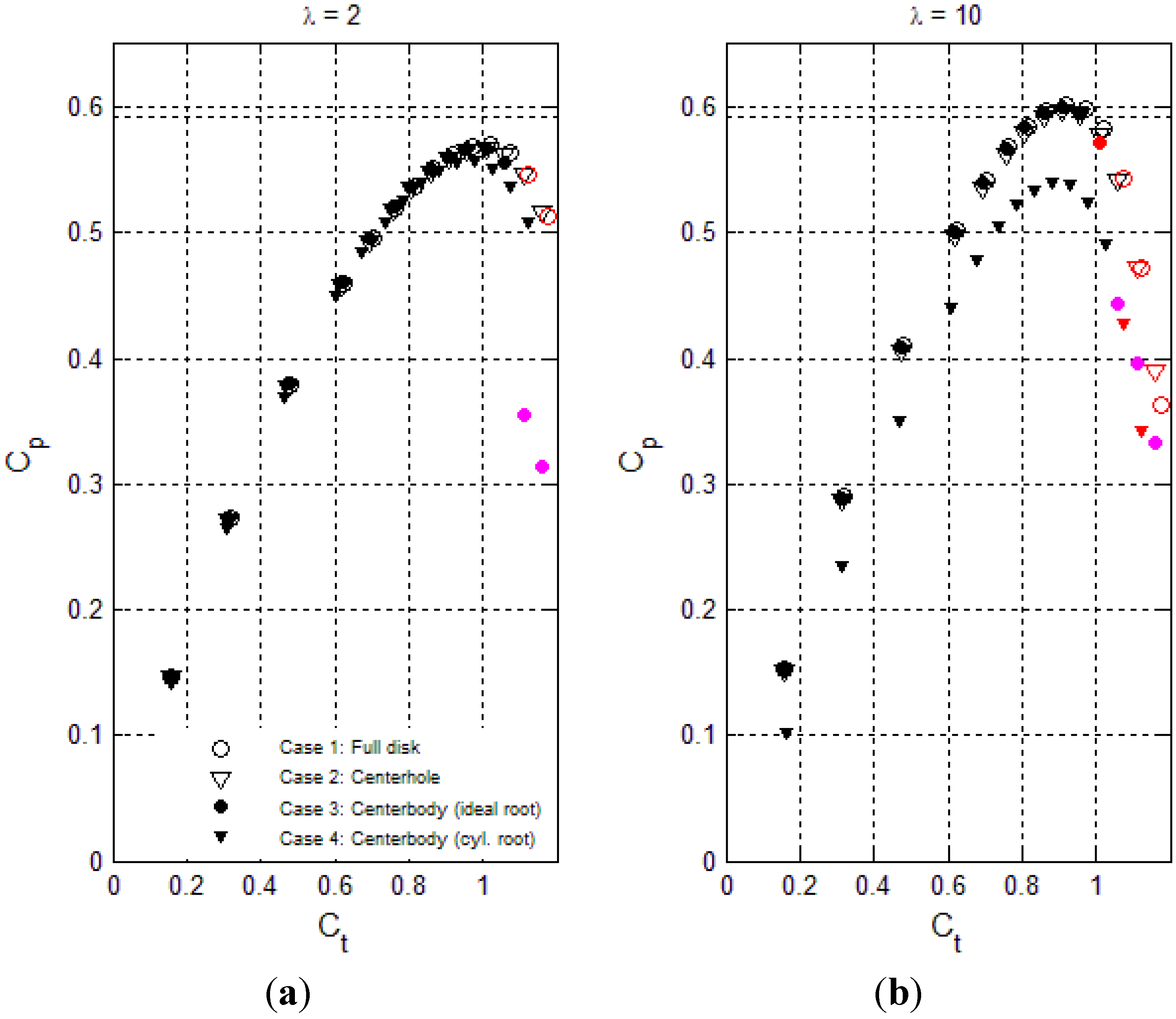
The AD CFD RANS results for the 112 HAWT runs are shown on Figure 15 and flow visualizations for the two TSR combinations of case 4 at peak power thrust loading condition are shown on Figure 16. Up to peak power thrust loading, the power performance is not affected by the type of nacelle/rotor, only exception being the centerbody w. cylinder root (case 4) for high TSR, where the drag force from the cylinder inner part of the rotor blades causes a CP loss of about 0.12. At highly loaded conditions beyond the power peak thrust loading, wake stall will gradually set in for the uniformly loaded cases 1,2 without centerbody, but without causing a distinct power drop, and most so for TSR = 10. The only distinct power drops are noticed for case 3, where the pressure drop across the inner part of the highly loaded rotor leads to a steep pressure recovery along the centerbody surface, ultimately causing centerbody surface stall. Especially for the high swirl TSR of 2. This seems to agree qualitatively with the tendency observed by Clausen et al. for swirled nozzle flows [36] that high swirl can promote inner core vortex break-down. However, case 4 for the high swirl TSR of 2 is the most stall resistant of all eight configurations. It seems that the ramped-down thrust loading towards the blade root causes the disk pressure drop and subsequent pressure recovery along the centerbody surface to be avoided or at least alleviated. When case 4 is most stall resistant with the high swirl TSR of 2 and not with the low swirl TSR of 10, this could stem from the increased swirl-induced mass-flow at the center, which in combination with the expansion of the surrounding wake causes a sustained low pressure along and past the centerbody, thereby reducing the risk of surface stall and/or vortex breakdown. Relevant monitoring of the pressure coefficient along the straight part of the centerbody will be presented and discussed later in this section. In summary the results confirm that stall scenarios only appear at post-power-peak thrust loadings, and that very different HAWTs therefore in general have a robust power production. The tendency of the high-swirl configurations to be more stall resistant at post-power-peak conditions should also be noted.
Figure 14.
(a) HAWT example of inner wake stall (sometimes termed “vortex breakdown”) at ; (b) DAWT example of centerbody stall at .
Figure 14.
(a) HAWT example of inner wake stall (sometimes termed “vortex breakdown”) at ; (b) DAWT example of centerbody stall at .

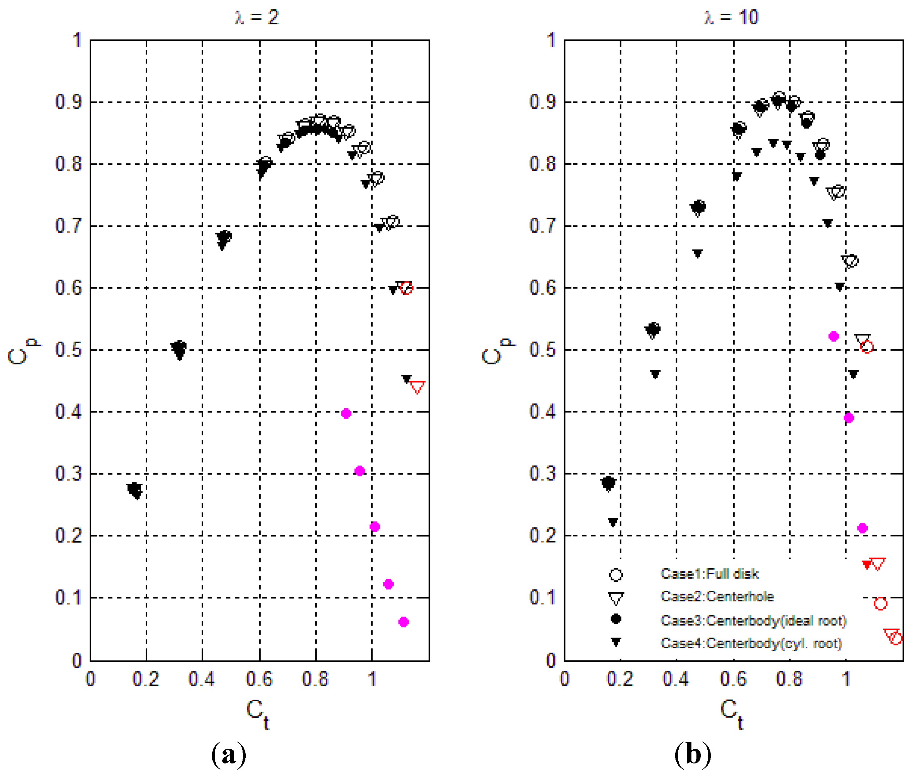
The AD CFD RANS results for the 112 Hansen DAWT runs are shown on Figure 17 and case 4 selected flow visualizations at peak power loading on Figure 18. Hansen [21] calculated a peak power CP of 0.93 for same and infinite TSR. The present peak power CP for the full disk (case 1) and TSR = 10 is 0.91, which agrees quite well considering the different TSRs and other minor differences, e.g., the turbulence model. Again, we see that the power performance is not significantly affected by the type of nacelle/rotor up to the power-peak thrust loading, with the exception of the centerbody with cylinder root (case 4) for high TSR, where inner blade cylinder drag causes a CP loss of about 0.13.
Figure 15.
Rotor CT – CP performance plots for four different HAWT nacelle/rotors. (a) Low TSR = 2; (b) High TSR = 10.
Figure 15.
Rotor CT – CP performance plots for four different HAWT nacelle/rotors. (a) Low TSR = 2; (b) High TSR = 10.

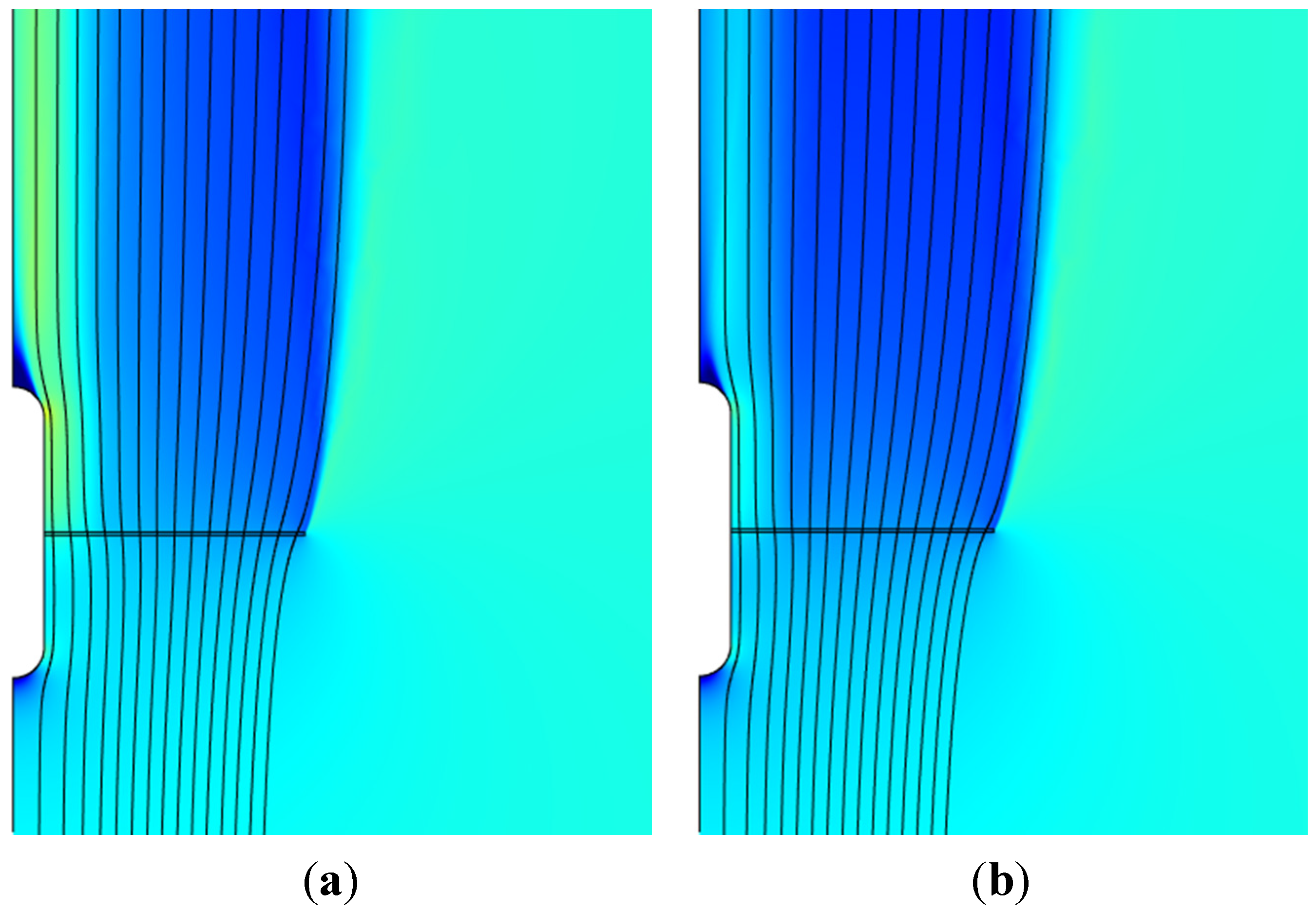
Figure 16.
Axial velocity and streamlines. . (a) TSR = 2; (b) TSR = 10. HAWT. Nacelle/rotor: Centerbody with cylindrical root section.
Figure 16.
Axial velocity and streamlines. . (a) TSR = 2; (b) TSR = 10. HAWT. Nacelle/rotor: Centerbody with cylindrical root section.

The same high-load tendencies as for the HAWT are noted: 1) Gradual power decrease for the cases 1–2 without centerbody, and generally earlier onset of wake-stall for the low swirl TSR of 10. 2) Distinct power drop for the case 3 centerbody with uniform ideal thrust loading, especially for the high swirl TSR of 2. 3) The very stall-resistant power performance of the case 4 centerbody with ramped-down center loading and low TSR of 2. Although these tendencies are similar to the HAWT findings, it is seen that the power decrease is more abrupt for the Hansen DAWT. In particular the case 3 high swirl configuration experiences a sudden onset of centerbody surface stall and subsequent 50+ percent power drop at . Such pronounced stall close to the peak-power loading at might be problematic, and dynamic stall-hysteresis effects could be hypothesized to cause a hanging stall condition. This would be a relevant issue for further investigations. In summary the results show that stall scenarios only appear at post-power-peak thrust loadings, but with a steeper power drop than for the HAWT, especially for the case 3 centerbody with uniform loading configurations. Again, the power-drops caused by the centerbody surface stall in case 3 is completely removed for the high swirl TSR of 2 when the loading of the inner part of the rotor is ramped down to zero towards the root (case 4).
The AD CFD RANS results for the 112 multi-element DAWT runs are shown on Figure 19 and case 4 selected flow visualizations at peak power loading on Figure 20. The tendencies from the HAWT and Hansen DAWT results are repeated again, but are this time very pronounced so that strong observations can be stated:
- As long as stall is avoided, the power performance is not sensitive to the type of nacelle/rotor, only exception being case 4 (centerbody with ramped-down inner loading) which performs about 0.08 lower in CP for TSR = 10 due to inner-blade cylinder drag.
- For the nacelle/rotor cases 1–2 without centerbody, the onset of inner wake stall comes at post-power-peak loading, and at lower loading for the low swirl TSR of 10 than for the high swirl TSR of 2.
- Centerbody surface stall for case 3 (centerbody, uniform disk loading) occurs at pre-power-peak thrust loading, both for high and low swirl, and most pronounced for high swirl TSR of 2.
- Very stall-resistant power performance of case 4 centerbody with ramped-down center loading and low TSR of 2.
The combination of high swirl (low rotor TSR) and ramped-down rotor thrust loading towards the disk center (case 4) seems to work well for all three WTG configurations, and in particular so for the multi-element DAWT. This observation does not follow intuitively from the related expanding nozzle flow results by Clausen et al. [36] from which one would expect high swirl configurations to be more prone to core vortex breakdown. Further insight is obtained by monitoring the pressure coefficient distributions along the straight part of the centerbody surfaces for case 4, as shown in Figure 21, and will be discussed in the following. The pressure drop across the disk from the cylinder blade roots due to drag occurs at axial position. The pressure coefficient follows standard definition, .
Figure 17.
Rotor CT – CP performance plots for four different Hansen diffuser augmented wind turbines (DAWT) nacelle/rotors. (a) Low TSR = 2; (b) High TSR = 10.
Figure 17.
Rotor CT – CP performance plots for four different Hansen diffuser augmented wind turbines (DAWT) nacelle/rotors. (a) Low TSR = 2; (b) High TSR = 10.

Figure 18.
Axial velocity and streamlines. . (a) TSR = 2; (b) TSR = 10. Hansen DAWT. Nacelle/rotor: Centerbody with cylindrical root section.
Figure 18.
Axial velocity and streamlines. . (a) TSR = 2; (b) TSR = 10. Hansen DAWT. Nacelle/rotor: Centerbody with cylindrical root section.
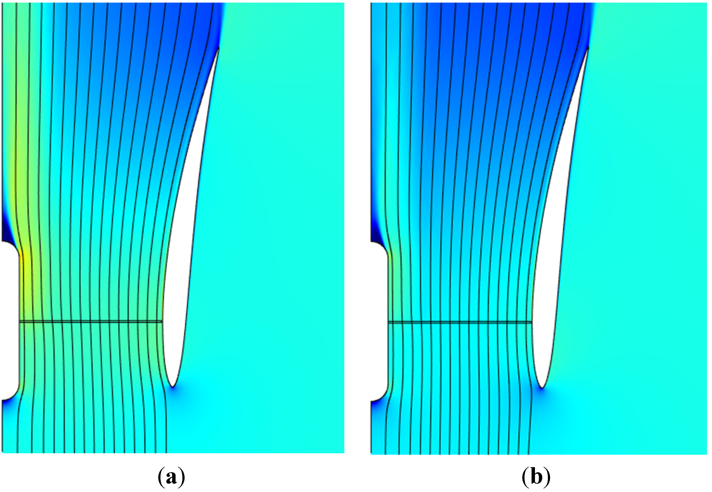
Figure 19.
Rotor CT – CP performance plots for four multi-element DAWT nacelle/rotors. (a) Low TSR = 2; (b) High TSR = 10.
Figure 19.
Rotor CT – CP performance plots for four multi-element DAWT nacelle/rotors. (a) Low TSR = 2; (b) High TSR = 10.

Figure 20.
Axial velocity and streamlines. (a) TSR = 2, ; (b) TSR = 10, . Multi-element DAWT. Nacelle/rotor: Centerbody with cylindrical root section.
Figure 20.
Axial velocity and streamlines. (a) TSR = 2, ; (b) TSR = 10, . Multi-element DAWT. Nacelle/rotor: Centerbody with cylindrical root section.
The centerbody pressure distributions downstream of the disk for the HAWT on the upper plots are neutral at low thrust loading, and become increasingly favorable with increasing disk loading. A favorable pressure gradient on a straight surface will prevent boundary layer flow reversal and surface stall. Upon further disk loading beyond the peak-power stall will ultimately take place, but it will be a gentle wake stall, not an abrupt centerbody surface stall, see, e.g., Figure 15b, case 4. Also note that swirl-induced core flow augmentation and pressure drop is higher for TSR = 2 (left plot), leading to lower surface pressure and higher favorable pressure gradient, than for TSR = 10 (right). The blue straight lines are tangents to the highest (i.e., most adverse) local pressure gradients on the curves for the peak-power thrust load cases ().
Figure 21.
Pressure coefficient distributions along axial part of centerbody for different TSR and CT. Nacelle/rotor: Centerbody with cylindrical root section. Left: . Right: . (a) HAWT; (b) Hansen DAWT; (c) Multi-element DAWT.
Figure 21.
Pressure coefficient distributions along axial part of centerbody for different TSR and CT. Nacelle/rotor: Centerbody with cylindrical root section. Left: . Right: . (a) HAWT; (b) Hansen DAWT; (c) Multi-element DAWT.
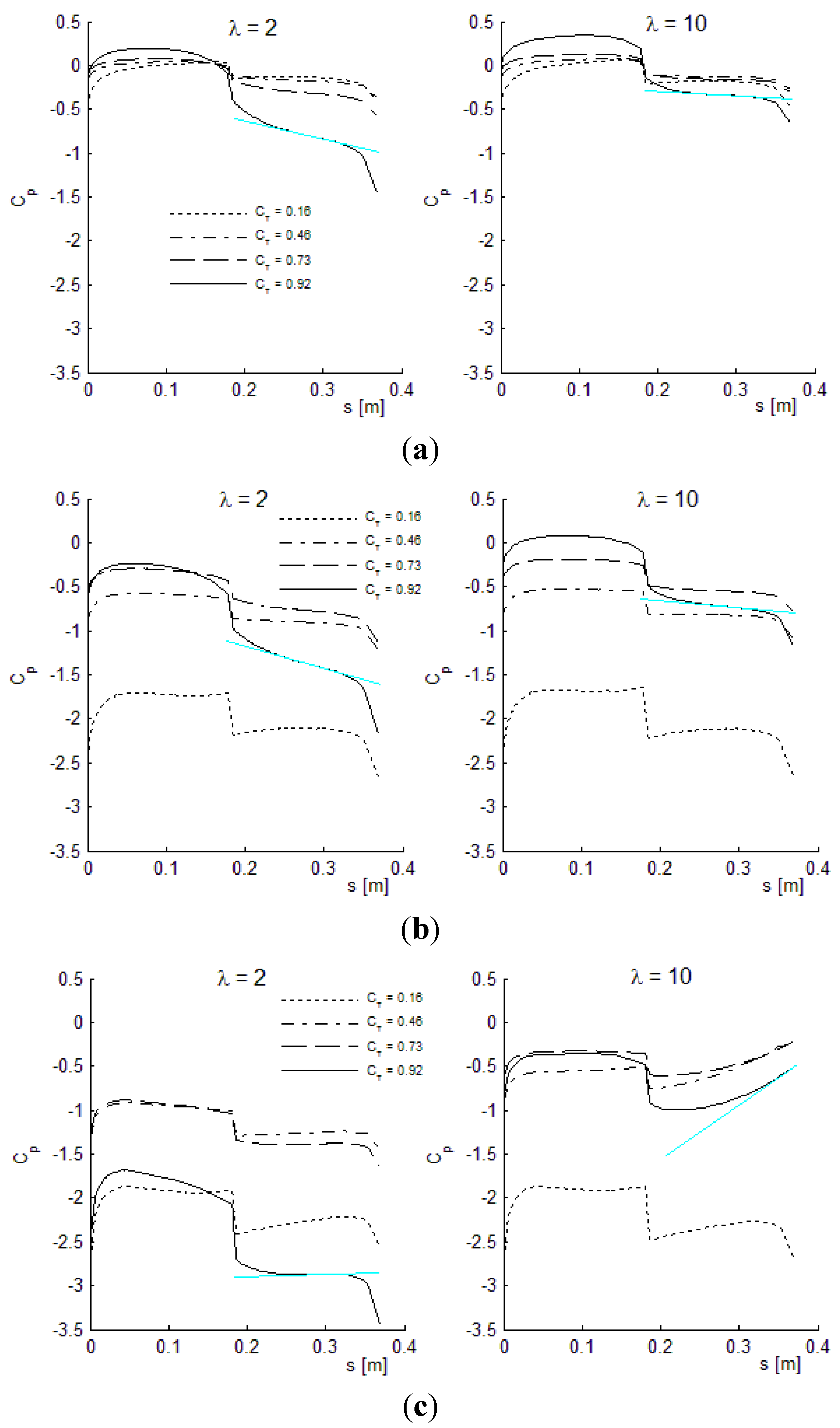
The mid plots on Figure 21 are for the Hansen diffuser. At low loading the downstream pressure gradient is mostly neutral or slightly adverse locally. The gradients will become favorable with increasing thrust loading, especially for the high swirl configuration with a TSR of 2 (left) due to the center wake pressure drop mechanism. At very high loading a gentle wake stall will occur as seen from Figure 17b, case 4.
The lower plots on Figure 21 are for the high-performing multi-element diffuser. At low loading () there is not much swirl and expansion from the surrounding wake to accelerate the core flow. The high diffuser expansion angle will therefore dominate the core flow and create the adverse pressure gradient observed for both TSRs. With increasing loading (), the high swirl configuration for TSR of 2 will gradually increase the core pressure drop, and neutralize the pressure gradient. At still higher loads () the pressure gradient will be mostly favorable. The low swirl case with TSR of 10 will, upon increased loading, not benefit as much from a swirl-induced core pressure drop, and therefore fall into a centerbody surface stall condition, leading to a significant power drop, see Figure 19b, case 4.
Table 3 contains a summary of the power-optimal performance from Figure 15, Figure 17, and Figure 19, cases 3–4. Cases 1–2 are left out because the idealized lack of a centerbody is not relevant for realistic physical applications.
| Configuration | |||||
|---|---|---|---|---|---|
| Bare HAWT, ideal root | 2 | 0.57 | 0.57 | 0.96 | 0.96 |
| 10 | 0.60 | 0.60 | 1.01 | 1.01 | |
| Bare HAWT, cyl. root | 2 | 0.56 | 0.56 | 0.94 | 0.94 |
| 10 | 0.54 | 0.54 | 0.91 | 0.91 | |
| Hansen DAWT, ideal root | 2 | 0.86 | 0.46 | 1.45 | 0.78 |
| 10 | 0.90 | 0.49 | 1.52 | 0.82 | |
| Hansen DAWT, cyl. root | 2 | 0.86 | 0.48 | 1.44 | 0.78 |
| 10 | 0.83 | 0.47 | 1.41 | 0.76 | |
| Multi-element DAWT, ideal root | 2 | 1.26 | 0.67 | 2.12 | 1.12 |
| 10 | 1.25 | 0.66 | 2.10 | 1.11 | |
| Multi-element DAWT, cyl. root | 2 | 1.62 | 0.86 | 2.73 | 1.45 |
| 10 | 1.13 | 0.60 | 1.90 | 1.01 |
Appendix 2 contains complementary analysis on the centerbody surface stall mechanisms. The downstream centerbody pressure gradient correlation is quite clear as already seen. But it should also be noted that uniform loading of the disk with centerbody (case 3) in combination with high swirl (TSR of 2) creates a strong inner core swirl adjacent to the centerbody surface. In combination with the high diffuser expansion angle on the multi-element diffuser, a premature centrifugal-type centerbody surface stall is observed at premature load levels, see Figure A2a. This stall scenario resembles the classical core vortex breakdown of swirled flows through expanding nozzles [35,36]. We can summarize that high-performance diffusers are challenged on the adverse pressure gradient occurring through the inner core flow downstream of the disk, especially in the presence of a centerbody that easily can promote centerbody surface stall and associated power drop. Key ingredients to the successful avoidance of premature stall and loss of shaft power are the swirl-induced core pressure drop and the uneven rotor loading, where the otherwise constant thrust level is ramped down to zero at the blade roots on the inner, say, 30% of the blades. Failure to operate with sufficiently low TSR will cause an axially adverse pressure gradient on the centerbody and high risk of surface stall. Failure to ramp down the loading on the inner part will cause concentrated core vorticity and a centrifugal-type centerbody flow separation.
Power efficiency is evaluated based on rotor area as is common for HAWTs, but also based on the projected diffuser area or “exit area” which is the maximum area covered by the diffuser circumference measured perpendicular to the axis of symmetry. Regarding the multi-element DAWT, the high performance, both by the “rotor” and “exit” area metric, is observed. The loss of energy associated with too little swirl-induced core flow augmentation and/or too concentrated inner core swirl should also be highlighted.
With CT and CL close to unity, a TSR as low as 2 will make the blades become very broad. This is feasible for small wind applications but not for large wind turbines. Small WTG blades operate at lower Reynolds number and lower L/D ratios. Therefore, we can at this stage skip the infinite L/D assumption and make a qualified estimate of a small blade operating with a L/D ratio of roughly 40. Recalculating the AD RANS CFD runs from Table 3 with this finite L/D ratio gives the results presented in Table 4. The shaft power performance of the small low TSR multi-element DAWT is more than 50% higher than the HAWT based on exit area, and more than 180% higher based on rotor area.
| Configuration | |||||
|---|---|---|---|---|---|
| Bare HAWT, ideal root | 2 | 0.53 | 0.53 | 0.89 | 0.89 |
| 10 | 0.45 | 0.45 | 0.75 | 0.75 | |
| Bare HAWT, cyl. root | 2 | 0.52 | 0.52 | 0.87 | 0.87 |
| 10 | 0.39 | 0.39 | 0.65 | 0.65 | |
| Hansen DAWT, ideal root | 2 | 0.81 | 0.44 | 1.37 | 0.74 |
| 10 | 0.77 | 0.42 | 1.30 | 0.70 | |
| Hansen DAWT, cyl. root | 2 | 0.81 | 0.44 | 1.37 | 0.74 |
| 10 | 0.70 | 0.38 | 1.19 | 0.64 | |
| Multi-element DAWT, ideal root | 2 | 1.19 | 0.63 | 2.01 | 1.07 |
| 10 | 1.13 | 0.60 | 1.91 | 1.01 | |
| Multi-element DAWT, cyl. root | 2 | 1.53 | 0.81 | 2.58 | 1.37 |
| 10 | 0.97 | 0.51 | 1.64 | 0.87 |
As a consequence of the needed flow stabilization effect from high swirl, successful high-performance DAWT applications should employ low TSR rotors. An approximate, yet useful, expression for the local blade solidity as a function of rotor design CT, blade design CL, and λ is given below.
5. Discussion, Conclusions, and Perspectives
Two flow mechanisms that contribute to create an adverse pressure gradient along the WTG centerbody surface leading to premature flow separation and wake stall have been identified: even rotor loading and normal/high tip-speed-ratios. The centerbody adverse pressure gradient problem worsens with increasing flow augmentation capability of the diffuser. It is very likely that these stall-mechanisms have played a role in earlier failed attempts to commercialize DAWTs, in particular those with high diffuser expansion angles, such as the latest generation Vortec7 designs [12], where the different stall scenarios were in fact identified, but never satisfactorily remedied: The rotor blades maintained their thrust loading capability all the way inboards to the root (no off-loading cylinder root), and the TSRs of 5–7 were not low enough to ensure sufficient swirl-induced core pressure drop. Furthermore, in earlier investigations, the upscaling from tunnel test scale-model to prototype has typically involved increased TSR due to structural load alleviation and CoE considerations. The fact that increasing TSR reduces swirl and thereby the resistance to stall-induced power drops for high performance diffusers has never been taken into account in previous DAWT research. If this issue is not addressed specifically during rotor design, the consequence would be that only diffusers with low flow augmentation capability will avoid premature stall. This would be an unattractive trade-off, since the whole idea of the diffuser is to maximize the flow augmentation. The key rotor design features to ensure a neutral or favorable pressure gradient along the DAWT centerbody (nacelle) and consequently avoid separation and stall are: (1) use of very low tip-speed-ratios for turbine operation, which creates a reduced back pressure of the inner part of the near wake due to high swirl. (2) a distinct uneven rotor loading which ramps down towards zero at the blade root. Apart from alleviating the pressure drop across the inner part of the rotor disk in the vicinity of the centerbody surface, the expansion of the wake behind the fully loaded outer part of the disk will narrow the inner wake confined space causing a speed-up and sustained low-pressure further downstream in the inner wake beyond the critical rear end of the centerbody.
5.1. Conclusions regarding BEM Models:
- The standard BEM model with no inclusion of the far-wake pressure drop term fails to predict any inner wake mass-flow increase due to finite TSR.
- The BEM with correct inclusion of the far-wake pressure drop predicts the swirl-induced core flow augmentation and compares well with AD results.
- The simplified inclusion of the far-wake pressure drop term (Burton, [23]) leads to a reasonable prediction of the inner wake mass-flow increase. While this BEM method is slightly less accurate than with the full wake pressure drop inclusion, the benefit of maintaining tube-element independency makes it recommendable for most engineering use.
5.2. Conclusions regarding DAWT Rotor Design
- Rotors for diffusers with high capacity for flow augmentation must be designed with low operating TSR in order to avoid premature stall-induced power drops.
- The blade loading distribution for a rotor operating inside a high capacity diffuser, such as the multi-element diffuser, must be uneven, with very little or no loading on the most inboard part.
- Power efficiency of the multi-element DAWT with a TSR of 2, uneven loading, and small wind , will exceed HAWT CP and by more than 180% and 50% respectively.
The discovery of success/failure criteria for high-capacity DAWTs and the strong dependency on proper rotor design allows us to consider the implications for the high capacity DAWT from a commercial point of view.
5.3. Perspectives
- Small Wind: The need for a wake core mass-flow increase makes a low rotor TSR imperative. A low TSR of, e.g., 2 will make the turbine aero-acoustically inaudible. This no-noise property is a significant upside for household DAWTs, and could enable the penetration of such WTGs into suburban areas. The partial shielding of the rotor is also visually attractive. The combination of high rotor solidity and a very short multi-element diffuser renders sideways furling to be considered for turbine control, as it will protect the rotor by facing the extreme winds with the “slim” side of the diffuser.
- High wind: The need of high-capacity DAWTs to operate at low TSRs leads to broader blades and heavier loads. While the need for structural stiffness is easily and affordably dealt with for small house-hold turbines, it is different for large wind, where turbine cost scales almost linearly with material usage and principal load levels. This will affect CoE negatively. Therefore, the high-capacity DAWT does not seem attractive for large wind applications.
Author Contributions
Søren Hjort has written the article and performed the calculations. Helgi Larsen has guided the overall innovative process.
Conflicts of Interest
The authors declare no conflict of interest.
Nomenclature
Latin Symbols
| Area of stream-tube through disk at disk | [m2] | |
| Far-wake area of stream-tube through disk | [m2] | |
| Far upstream area of stream-tube through disk | [m2] | |
| Airfoil chord length | [m] | |
| Circular cylinder chord length | [m] | |
| Drag coefficient of circular cylinder section | ||
| Lift coefficient of airfoil section | ||
| Rotor (disk) axial thrust coefficient | ||
| Rotor (disk) power coefficient, all forces | ||
| Pressure coefficient on centerbody straight surface | ||
| Rotor (disk) power coefficient, axial forces only | ||
| Rotor (disk) power coefficient based on diffuser exit area | ||
| Rotor (disk) power coefficient, tangential forces only | [v] | |
| Airfoil drag force | [N] | |
| Airfoil drag force from disk on fluid | [N] | |
| Airfoil lift force from disk on fluid | [N] | |
| Thrust force from disk on fluid | [N] | |
| Thrust force from circular cylinder part | [N] | |
| Radial force from disk on fluid | [N] | |
| Force per disk volume | [N/m3] | |
| Tangential force from disk on fluid | [N] | |
| Airfoil lift force | [N] | |
| Axial length of diffuser | [m] | |
| based on rotor area normalized with Betz number | ||
| based on diffuser exit area norm. with Betz num. | ||
| Number of blades in rotor disk | ||
| Fluid static pressure | [Pa] | |
| Fluid static pressure in front of disk | [Pa] | |
| Fluid static pressure just behind disk | [Pa] | |
| Fluid static pressure at far-wake | [Pa] | |
| Fluid static ambient pressure at far-field | [Pa] | |
| Radial dimension measured from center-axis | [m] | |
| Rotor tip radius measured from center-axis | [m] | |
| Diffuser maximum radius measured from center-axis | [m] | |
| Reynolds number | ||
| Far-wake radius | [m] | |
| Centerbody straight surface length | [m] | |
| Axial velocity of flow through disk (AD) | [m/s] | |
| Normalized axial velocity of flow through disk (BEM) | ||
| Axial velocity of flow through disk (BEM) | [m/s] | |
| Axial velocity at far-wake (BEM) | [m/s] | |
| Tangential velocity of flow through disk (BEM) | [m/s] | |
| Normalized tangential velocity at far-wake (BEM) | ||
| Tangential velocity at far-wake (BEM) | [m/s] | |
| Free stream fluid velocity | [m/s] | |
| Volume | [m3] | |
| Tangential velocity of flow at disk (AD) | [m/s] | |
| Inflow velocity magnitude in rotating blade’s reference | [m/s] | |
| Weight factor for blade with lift forcing | ||
| Weight factor for cylinder root with drag forcing | ||
| Non-dimensional wall distance |
Greek Symbols
| Boundary mesh 1st row quad element height above wall | [m] | |
| Rotating reference disk angle with incoming flow | [rad] | |
| Fluid density | [kg/m3] | |
| Blade solidity at given radius | ||
| Rotor (disk) tip-speed-ratio | ||
| Disk rotational velocity | [rad/s] |
Abbreviations
| AD | Actuator Disk |
| BEM | Blade-Element Momentum |
| CFD | Computational Fluid Dynamics |
| CoE | Cost of Energy |
| DAWT | Diffuser-Augmented Wind Turbine |
| HAWT | Horizontal-Axis Wind Turbine |
| LHS | Left-Hand Side |
| NS | Navier-Stokes |
| RANS | Reynolds-Averaged Navier-Stokes |
| RHS | Right-Hand Side |
| WTG | Wind Turbine Generator |
Appendix 1
A1.1. Reduction of Variables for the Swirled-Flow BEM Formulation
The reduction of variables from Equations (2)–(10) to a closed-form analytical expression for Uw is shown below.
Elimination of and in the momentum conservation Equations (3) and (4) through use of mass conservation Equations (7) and (8):
Elimination of and through use of the Bernouilli state Equations (9) and (10), upstream and downstream of rotor:
RHS of Equations (A1) and (A4) are equal:
Ratio of RHS of Equations (A1) and (A2) equals RHS of Equation (5), leading to:
RHS of Equation (A5) is identical to LHS of Equation (A6) yielding:
The Equations (2)–(10) have at this point been reduced to Equation (A7), which states a rather simple relationship between the far wake axial and azimuthal velocity. Isolating Uw on the LHS leads to Equation (11), repeated below:
A1.2. Iterative Solution Scheme for the Swirled-Flow BEM Formulation
Without inclusion of the far-wake pressure term due to swirl, Δpw, Equation (A8) could be solved directly for each tube element. Δpw will normally have a non-dominant impact, even for small TSRs with increased swirl, and a simple iterative scheme will yield smooth and fast convergence. The algorithm used for computing the converged flow field variables for all tube elements is described below.
- Initialization: Set , , and . Remaining unknowns are zero. A priori known parameters are , λ, ρ, R, plus the forcing, e.g., by specifying the axial thrust coefficient distribution, , across the radial range.
- Update rw for the far-wake stream tube corresponding to each element including Rw for the outermost stream tube, using the mass conservation property along with current values for Ud and Uw.
- Loop over all tube elements starting at the outermost element
- a
- Update Δpw using Equation (2).
- b
- Compute a range of corresponding values for Uθw, Uw, and CT using Equations (11) and (12).
- c
- Compute values for Uθw and Uw at the target CT value (specified forcing) by interpolation.
- d
- Compute Ud using Equation (A6).
- Check for convergence of the flow variables, Uw, Uθw, and Ud on all tube elements. If no convergence, goto 2).
- Solution successfully completed. Post-process by calculating all local thrust and power coefficients using Equations (12)–(15). Also calculate the area-integrated average values for thrust and power coefficients.
The algorithm is robust, although a converged solution for tube elements sufficiently close to the center-axis for small values of cannot be guaranteed. The critical value for will depend on the TSR value, λ, but is below 0.025 for TSRs down to 2. Below , the inner-core tube element relative radius must be slightly larger than 0.025, or otherwise a more robust iteration scheme should be used. Alternatively, a gradual thrust unloading close to the center-axis would also enable inner-core convergence for TSRs below 2.
A1.3. Addition of Drag Forces in the Swirled-Flow BEM Formulation
The introduction of a finite ratio between the lift force and the drag force exerted by the blade on the fluid (L/D for brevity) leads to a modified formulation. The added complexity is showed on the right drawing of Figure 2. Equation (5) in the ideal formulation with infinite L/D is now replaced by:
Note that Equation (5) is recovered from Equation (A9) as L/D approaches the ideal inviscid limit. The equivalent to Equation (11) for finite L/D becomes:
The 3rd (lengthy) term of Equation (A10) contains Ud which in principle complicates the solution procedure. Former iteration loop values for Ud must now be used for the evaluation of the RHS of (A10). Fortunately the impact from on the 3rd term is small as long as the L/D ratio is fairly large, so the proposed solution scheme converges rapidly.
Appendix 2
An adverse pressure gradient along a straight surface is known to have a significant impact on the development of boundary layer flow reversal and separation. Iso-pressure contours over the centerbody are shown for the multi-element DAWT at low thrust loading, Figure A1, and medium thrust loading, Figure A2.
Figure A1.
Low loading: Streamlines and fixed-range selection of pressure contour lines for the multi-element DAWT at a low CT thrust loading of 0.32. Left plots: TSR = 2. Right plots: TSR = 10. Upper plots: Ideal inner-blade section with constant thrust loading (case 3). Lower plots: Cylindrical inner-blade section with drag and ramped-down thrust loading (case 4). In the presence of a sufficiently adverse pressure gradient on the centerbody surface downstream of the disk, flow separation (centerbody stall) will occur. Neutral pressure gradient along the centerbody is seen on case 3 with high swirl and low TSR of 2 (a). The most adverse pressure gradient is seen on case 4 with low swirl and high TSR of 10 (d), where flow separation will in fact occur when increasing CT from 0.32 to 0.48.
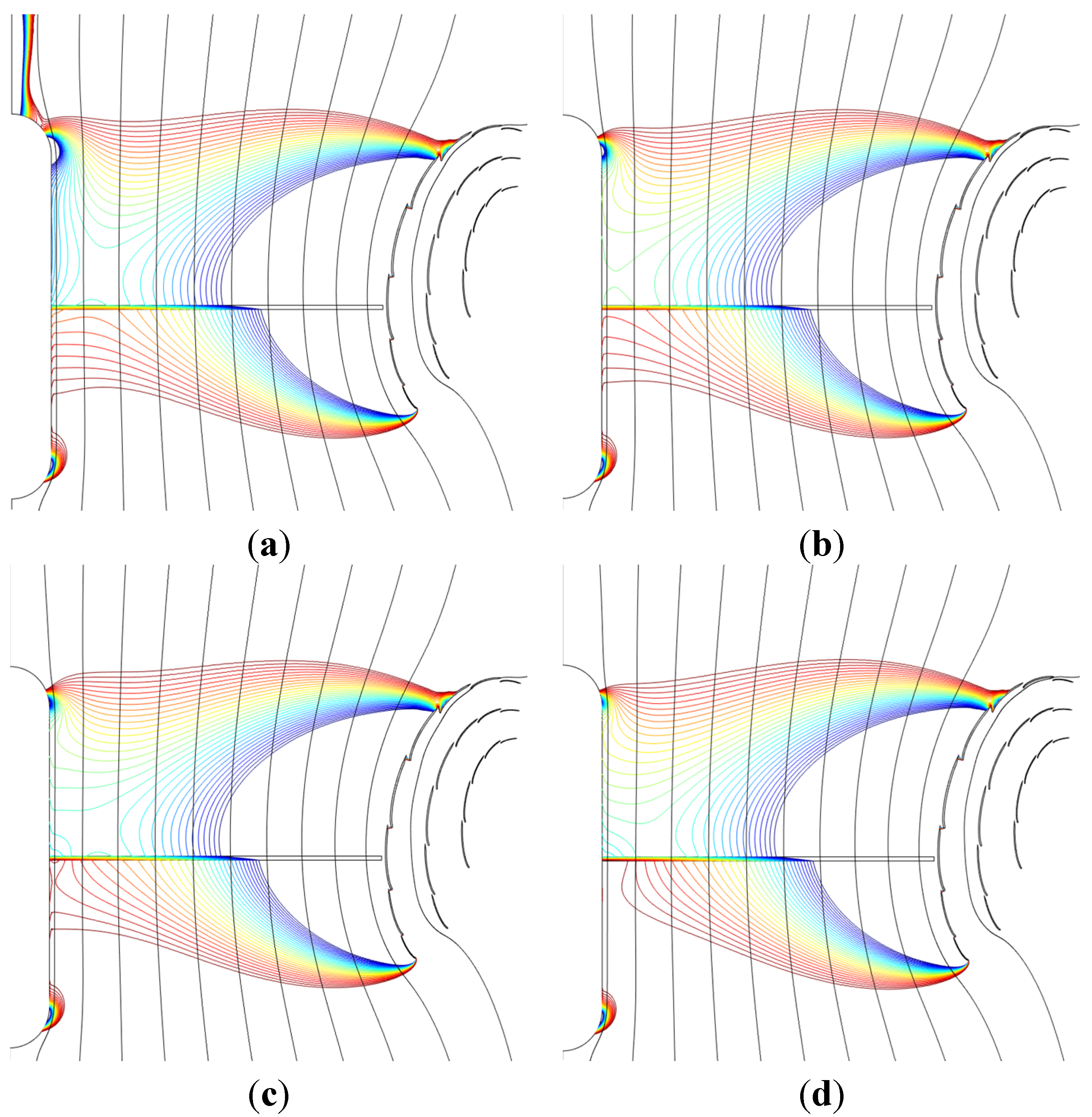
Figure A2.
Medium loading: Streamlines and fixed-range selection of pressure contour lines for the multi-element DAWT at a medium CT thrust loading of 0.61. Left plots: TSR = 2. Right plots: TSR = 10. Upper plots: Ideal inner-blade section with constant thrust loading (case 3). Lower plots: Cylindrical inner-blade section with drag and ramped-down thrust loading (case 4). When increasing CT to 0.75 both case 3 rotors (upper) will fall into stall, with deflected flow and power drop as already happened at low loading for case 4 at TSR = 10 (d). So, both upper case 3 flows are close to stall. In the low swirl configuration (right), the stall will be triggered by the adverse pressure gradient along the centerbody. In the high swirl configuration (left), the pressure gradient along the centerbody is actually slightly favorable, which should prevent boundary layer flow reversal and stall. A large radial gradient is seen, however, caused by the combination of high swirl and constant disk loading all the way in towards the root, which in combination with the centerbody boundary layer momentum loss will lead to a centrifugal type flow separation, probably not unlike the expanding nozzle vortex breakdowns reported in [35,36]. The only “healthy” configuration left is the case 4 high swirl flow (c) where axial flow augmentation is created but without the concentrated inner vortex, since the blades are gradually unloaded on the inner third spanwise range of the blades. No inner-swirl-induced radial pressure gradient is seen, and the axial pressure gradient is close to neutral. Further increase of the thrust loading will cause the axial pressure gradient along the centerbody downstream of the disk to become favorable. This is also apparent on Figure 21.

References
- Lilley, G.M.; Rainbird, W.J. A Preliminary Report on the Design and Performance of Ducted Windmills; Cranfield College of Aeronautics: Bedford, UK, 1956. [Google Scholar]
- Iwasaki, M. The Experimental and Theoretical Investigation of Windmills; Research Institute for Applied Mechanics, Kyushu University: Kyushu, Japan, 1953; Volume 2. [Google Scholar]
- Sanuki, M. Studies on biplane wind planes ventilation tubes and cup anemometers. Meteorol. Geophys. Jpn. 1950, 1, 279–290. [Google Scholar]
- Igra, O. Shrouds for aerogenerators. AIAA J. 1976, 14, 1481–1483. [Google Scholar] [CrossRef]
- Igra, O. Design and performance of a turbine suitable for an aerogenerator. Energy Convert. 1976, 15, 143–151. [Google Scholar] [CrossRef]
- Igra, O. Compact shrouds for wind turbines. Energy Convert. 1977, 16, 149–157. [Google Scholar] [CrossRef]
- Igra, O. The shrouded aerogenerator. Energy 1977, 2, 429–439. [Google Scholar] [CrossRef]
- Igra, O. Research and development for shrouded wind turbines. In Proceedings of the European Wind Energy Conference, Hamburg, Germany, 22–26 October 1984.
- Lewis, R.I.; Williams, J.E.; Abdelghaffar, M.A. A theory and experimental investigation of ducted wind turbines. Wind Eng. 1977, 1, 104–125. [Google Scholar]
- Oman, R.A.; Foreman, K.M.; Gilbert, B.L. Investigation of Diffuser Augmented Wind Turbines, Parts I and II; Grumman Research Department Report RE-534, ERDA Report C00–2616–2; Grumman Aerospace: New York, NY, USA, 1977. [Google Scholar]
- Gilbert, B.L.; Oman, R.A.; Foreman, K.M. Fluid dynamics of diffuser-augmented wind turbines. Energy 1978, 2, 368–374. [Google Scholar] [CrossRef]
- Phillips, D.G. An Investigation of Diffuser Augmented Wind Turbine Design. Ph.D. Thesis, University of Auckland, Auckland, New Zealand, 2003. [Google Scholar]
- Betz, A. Schraubenpropeller mit geringstem Energieverlust. Mit einem Zusatz von l. Prandtl. Nachr. Ges. Wiss. zu Göttingen Math.-Phys. Kl. 1919, 193–217. (In German) [Google Scholar]
- Glauert, H. The Elements of Aerofoil and Airscrew Theory; Cambridge University Press: Cambridge, UK, 1926. [Google Scholar]
- Wilson, R.E.; Lissaman, P.B.S. Applied Aerodynamics of Wind Power Machines; Oregon State University Report; Oregon State University: Corvallis, OR, USA, 1974. [Google Scholar]
- Van Bussel, G.J.W. An assessment of the performance of diffuser augmented wind turbines. In Proceedings of the 3rd ASME Joint Fluids Engineering Conference, San Francisco, CA, USA, 18–23 July 1999.
- Van Bussel, G.J.W. The science of making more torque from wind: Diffuser experiments and theory revisited. J. Phys. Conf. Ser. 2007, 75, 1–12. [Google Scholar] [CrossRef]
- Jamieson, P. Generalized limits for energy extraction in a linear constant velocity flow field. J. Wind Energy 2007, 11, 445–457. [Google Scholar] [CrossRef]
- Werle, M.; Presz, W. Ducted wind/water turbines and propellers revisited. Propuls. Power 2008, 24, 1146–1150. [Google Scholar] [CrossRef]
- Hjort, S.; Larsen, H. A multi-element diffuser augmented wind turbine. Energies 2014, 7, 3256–3281. [Google Scholar] [CrossRef]
- Hansen, M.O.L. Effect of placing a diffuser around a wind turbine. Wind Energy 2000, 3, 207–213. [Google Scholar] [CrossRef]
- Madsen, H.A.; Mikkelsen, R.; Øye, S.; Bak, C.; Johansen, J. A detailed investigation of the blade element momentum (BEM) model based on analytical and numerical results and proposal for modifications of the BEM model. J. Phys. Conf. Ser. 2007, 75. [Google Scholar] [CrossRef]
- Burton, T.; Sharpe, D.; Jenkins, N.; Bossanyi, E. Wind Energy Handbook; John Wiley and Sons Ltd.: Chichester, UK, 2001. [Google Scholar]
- Hansen, M.O.L. Aerodynamics of Wind Turbines, 3rd ed.; Routledge: New York, NY, USA, 2015. [Google Scholar]
- Ohya, Y.; Karasudani, T. A shrouded wind turbine generating high output power with wind-lens technology. Energies 2010, 3, 634–649. [Google Scholar] [CrossRef]
- Lyon, C.A.; Broeren, A.P.; Giguère, P.; Gopalarathnam, A.; Selig, M.S. Summary of Low-Speed Airfoil Data; SoarTech Publications; University of Illinois: Champaign, IL, USA, 1998; Volume 3. [Google Scholar]
- Wood, D. Small Wind Turbines: Analysis, Design, and Application; Springer: Berlin, Germany, 2011. [Google Scholar]
- Abbott, I.H.; von Doenhoff, A.E. Theory of Wing Sections; Dover: New York, NY, USA, 1959. [Google Scholar]
- Drela, M. XFOIL: An analysis and design system for low reynolds number airfoils. In Low Reynolds Number Aerodynamics; Springer-Verlag: Berlin/Heidelberg, Germany, 1989; pp. 1–12. [Google Scholar]
- Branlard, E. Analysis of Wind Turbine Aerodynamics and Aeroelasticity Using Vortex-based Methods. Ph.D. Thesis, Technical University of Denmark, Kongens Lyngby, Denmark, 2015. [Google Scholar]
- Mikkelsen, R. Actuator Disc Methods Applied to Wind Turbines. Ph.D. Thesis, Technical University of Denmark, Kongens Lyngby, Denmark, 2004. [Google Scholar]
- CFD Module User’s Guide, version 4.4; Comsol Inc.: Burlington, MA, USA, 2013.
- Guermond, J.L.; Minev, P.; Shen, J. An overview of projection methods for incompressible flows. Comp. Meth. Appl. Mech. Eng. 2006, 195, 6011–6045. [Google Scholar] [CrossRef]
- Glauert, H. The Analysis of Experimental Results in the Windmill Brake and Vortex Ring States of an Airscrew; HM Stationary Office: London, UK, 1926. [Google Scholar]
- Clausen, P.D.; Wood, D.H. A possible recirculation limit for expanding swirling flows. In Proceedings of the 10th Australasian Fluid Mechanics Conference, Melbourne, Australia, 11–15 December 1989.
- Clausen, P.D.; Koh, S.G.; Wood, D.H. Measurements of a swirling turbulent boundary layer developing in a conical diffuser. Exp. Therm. Fluid Sci. 1993, 6, 39–48. [Google Scholar] [CrossRef]
© 2015 by the authors; licensee MDPI, Basel, Switzerland. This article is an open access article distributed under the terms and conditions of the Creative Commons Attribution license (http://creativecommons.org/licenses/by/4.0/).
Share and Cite
MDPI and ACS Style
Hjort, S.; Larsen, H. Rotor Design for Diffuser Augmented Wind Turbines. Energies 2015, 8, 10736-10774. https://doi.org/10.3390/en81010736
AMA Style
Hjort S, Larsen H. Rotor Design for Diffuser Augmented Wind Turbines. Energies. 2015; 8(10):10736-10774. https://doi.org/10.3390/en81010736
Chicago/Turabian StyleHjort, Søren, and Helgi Larsen. 2015. "Rotor Design for Diffuser Augmented Wind Turbines" Energies 8, no. 10: 10736-10774. https://doi.org/10.3390/en81010736