Article

Ammonia/Ethanol Mixture for Adsorption Refrigeration

School of Engineering, Institute for Materials and Processes, the University of Edinburgh, Sanderson Building, King′s Buildings, Robert Stevenson Road, Edinburgh EH9 3FB, UK
*
Author to whom correspondence should be addressed.
Energies 2020, 13(4), 983; https://doi.org/10.3390/en13040983
Submission received: 29 January 2020 / Revised: 14 February 2020 / Accepted: 19 February 2020 / Published: 22 February 2020

Abstract

:
Adsorption refrigeration has become an attractive technology due to the capability to exploit low-grade thermal energy for cooling power generation and the use of environmentally friendly refrigerants. Traditionally, these systems work with pure fluids such as water, ethanol, methanol, and ammonia. Nevertheless, the operating conditions make their commercialization still unfeasible, especially owing to safety and cost issues as a consequence of the working pressures, which are higher or lower than 1 atm. The present work represents the first thermodynamic insight in the use of mixtures for adsorption refrigeration and aims to assess the performance of a binary system of ammonia and ethanol. According to the Gibbs’ phase rule, the addition of a component introduces an additional degree of freedom, which allows to adjust the pressure of the system varying the composition of the mixture. The refrigeration process was simulated with isothermal- isochoric flash calculations to solve the phase equilibria, described by the Peng-Robinson-Stryjek-Vera (PRSV) equation of state for the vapor and liquid phases and by the ideal adsorbed solution theory (IAST) and the multicomponent potential theory of adsorption (MPTA) for the adsorbed phase. In operating condenser and evaporator, pressure levels around atmospheric pressure can be achieved using an ammonia/ethanol mixture with a mole fraction of ethanol in the range of 0.70−0.75. A good agreement in the predictions of the adsorbed phase composition was also reported using the IAST and the MPTA methods.

1. Introduction

The growing awareness of global warming and the need for reducing carbon emissions has resulted in incentives to fully develop renewable energy conversion technologies including refrigeration and air conditioning [1]. Increasing attention has been given to processes using fluids with zero ozone depletion potential and low global warming potential [2]. In this context, adsorption refrigeration is very promising due to the utilization of natural and environmentally friendly refrigerants and to the capability to exploit low-grade heat, especially in places characterized by high solar radiation [3,4,5,6]. In recent years, adsorption refrigeration has been also proposed for aerospace applications thanks to the absence of an electrical compressor, making these systems vibration-free. Tzabar [7,8] developed a Joule–Thomson cryocooler able to work in the range of temperatures interesting for satellites, independent from any active control and highly reliable. Potential applications include the Cube Sats, a new generation of satellites used for monitoring the Earth conditions. The need to mitigate any thermal gradient within them for enhancing the resolution of the collected data makes adsorption compressors a viable solution, as they supply cooling power without causing further vibrations.
The reason that adsorption heat transformers are still not commercialized lies in their high costs which are mainly associated with the operational pressures, which in turn are strictly related to the operating fluid saturation temperatures. As extensively reported in the literature, the most significant physical properties in the choice of a refrigerant are the latent heat of vaporization (λvap) and the saturation pressure (Psat). Table 1 reports the relevant physical properties of the most common fluids used for refrigeration at 283 K. In a recent study by Santori and Di Santis [9], performances of the thermodynamic cycle were also related to the fluid critical temperature (Tcr), critical pressure (Pcr), critical density (ρcr), acentric factor (ω), and molar heat capacity of ideal gas at critical point (cp0,cr). This approach confirmed the advantage of using traditional fluids for adsorption refrigeration and showed that other fluids, such as isopropanol, have promising properties, anticipating values of coefficient of performance (COP) not far from ethanol and methanol (Table 1).
These fluids exhibit different saturation pressures at the same working temperature. Water is characterized by a low saturation pressure, which bounds the design to sub-atmospheric operating conditions, although it is attractive for its non-toxicity, non-flammability, high latent heat, and availability. The use of methanol or ethanol as alternatives to water enables higher but still sub-atmospheric working pressures while with ammonia, the cycle operates at pressures considerably higher than 1 atm. Pressures lower than the atmospheric pressure require expensive vacuum components and demand periodical vacuum-tightness checks. On the other hand, operating with pressures higher than the atmospheric pressure makes unavoidable the use of components with high metal thicknesses, especially in the adsorption heat exchangers. Such heat exchangers need to be cooled down and heated up, requiring a remarkable amount of sensible heat that is not directed to the adsorbent material. The decrease in thickness of the heat exchanger pipes can reduce the metal/adsorbent mass ratio up to 50% resulting in a COP increase of 0.1 [10].
With a pure fluid as refrigerant, once the working temperature has been chosen, the pressure level is univocally fixed. According to the Gibbs’ phase rule, the introduction of another component to the system adds a degree of freedom, so that by varying the composition of the mixture, the operating pressure can be adjusted to be close to atmospheric pressure. While adsorption heat transformers working with pure fluids as refrigerant have been widely investigated, the literature on mixtures is still poor. The existing publications are mainly focused on experimental studies and involve a small scientific community. Wang and Zhu [11] carried out experiments and modelled an apparatus for the characterization of a system working with a mixture of ammonia and water adsorbed on zeolite 13X. The weakness of their work lies in the evaluation of the COP as the authors did not include the mixing enthalpy in calculating the heat of adsorption. This term is in fact significantly non-linear for associating mixtures such as the ammonia/water system. Tzabar [12] applied the notions of pure fluid adsorption isotherms to derive the adsorption of mixtures using extended isotherm models. Taking into account the degree of approximation, the capability of working with pure fluid isotherm parameters allows a straightforward use of existing information in literature. In a following paper, Tzabar and Grossman [13] designed an adsorption Joule-Thompson cryocooler that works with nitrogen/methane and nitrogen/ethane mixtures. Their analysis showed clear limitations in the description of the equilibrium as they modelled the adsorption of mixtures through the extended Langmuir model without considering non-idealities occurring in the adsorbed phase.
To accurately evaluate the performance of an adsorption refrigeration process involving a mixture, a full thermodynamic cycle needs to be simulated in detail. A conventional process consists of an adsorption bed acting as a thermal compressor, a condenser, an evaporator, and a throttling valve connected as shown in Figure 1a. The thermodynamic cycle is depicted in the pressure-temperature-concentration (P-T-x) diagram in Figure 1b. The operational steps of the thermal adsorption compressor can be scheduled as:
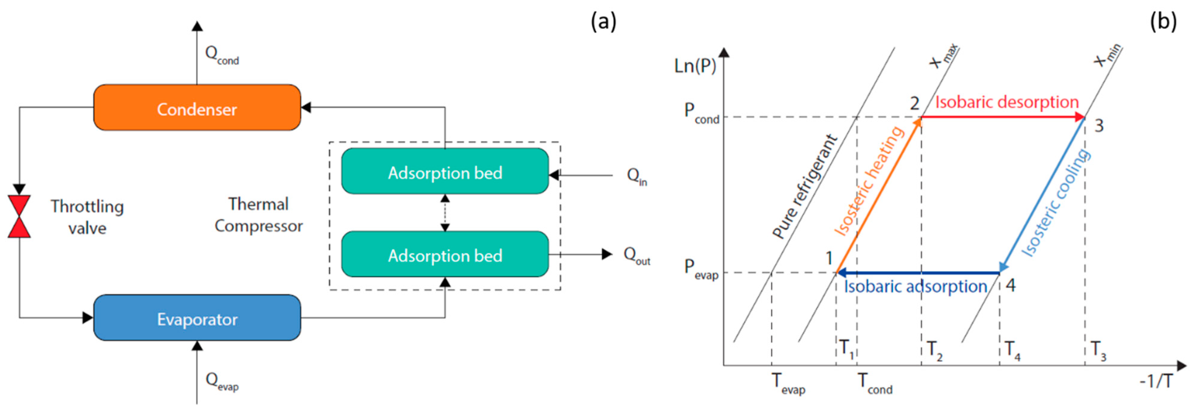
  • Isosteric heating (1−2): As a result of low-grade heating the pressure in the adsorption bed increases from Pevap to Pcond while the adsorption bed temperature increases from T1 to T2.
  • Isobaric desorption (2−3): The adsorption bed continues to receive heat and its temperature keeps raising from T2 to T3, which results in the desorption of the refrigerant vapor to the condenser under a constant vapor pressure. The working fluid concentration shifts from xmax to xmin.
  • Isosteric cooling (3−4): As a result of cooling, the pressure in the adsorption bed decreases from Pcond to Pevap while the adsorption bed temperature decreases from T3 to T4.
  • Isobaric adsorption (4−1): The adsorption bed continues to be cooled and its temperature keeps lowering from T4 to T1, which results in the adsorption of the refrigerant vapor from the evaporator under a constant vapor pressure. The working fluid concentration shifts back from xmin to xmax.
The present study aims to demonstrate the potential of using fluid mixtures instead of pure components as refrigerants so that the adsorptive refrigerators can work at pressures close to atmospheric pressure. The approach involves a rigorous thermodynamic framework to describe vapor-liquid equilibria in the evaporator and condenser as well as adsorption equilibria in the adsorption bed. This investigation is essential to clarify the limiting performance of the process excluding any transient phenomenon associated with heat and mass transfer. Within the scope of the present study, a mixture of ammonia and ethanol was selected. At the working temperatures of the condenser and the evaporator, ammonia shows a saturation pressure higher than 1 atm while ethanol shows a saturation pressure below 1 atm. Therefore, it is aimed to change the composition of the mixture to obtain an operating pressure close to atmospheric pressure and to assess the performance of the resulting refrigeration cycle.

2. Thermodynamic Model

As previously mentioned, equilibrium takes place between the vapor and liquid phases in both the evaporator and the condenser, while in the adsorption bed, the vapor phase is in equilibrium with the adsorbed phase within the solid phase, which does not actively take part in the process. When the evaporator, for instance, and the adsorption bed are connected and the thermodynamic equilibrium is established, the pressure and the vapor phase mole fractions are the same in the two vessels (Figure 2). Note that the vessels are at the different temperatures Tevap and Tads.
To model the vapor and liquid phases, the Peng-Robinson-Stryjek-Vera (PRSV) equation of state [14] was selected with a φ-φ approach. It has been reported that this equation works reasonably well in the vapor phase but reveals some weaknesses to predict the equilibrium of liquid phases containing associative compounds such as ammonia and ethanol [15]. Nevertheless, for the purpose of the present work, this deviation is taken as acceptable. This was checked in an analysis of the vapor–liquid equilibrium data against the proposed model in the range of compositions, pressure, and temperatures of interest. To model the adsorbed phase, two approaches were followed, and two case studies were accordingly designed. In case study A, the ideal adsorbed solution theory (IAST) was considered [16]. IAST is the most widespread theory for multicomponent adsorption interpretation and it postulates the existence of an adsorbed phase, which behaves as a Raoult’s ideal solution [17]. For this case, the three connections proper of a single-bed adsorption cycle were simulated, namely adsorption bed/evaporator, adsorption bed/condenser, and evaporator/condenser connections. Simulations took into account several initial compositions of the refrigerant mixture and multiple cycles were run until the convergence of the pressures in the condenser and in the evaporator was achieved. In case study B, the multicomponent potential theory of adsorption (MPTA) was implemented [18] focusing only on the connection between the evaporator and the adsorption bed. The two adsorption models were also compared in terms of prediction of the adsorbed phase mole fractions at equilibrium.

2.1. Case Study A: Complete cycle modelling with PRSV + IAST

In the single-bed adsorption cycle, there are three vessel connections to model. For each of them, the thermodynamic equilibrium is solved through a system of non-linear algebraic equations.
(a) Adsorption bed/Evaporator connection: In this stage, the valve between the adsorption bed and the evaporator is open and the vapor generated in the evaporator is adsorbed in the bed. The modelling of this connection can be extended from our previous works [19,20] based on ideal and non-ideal isothermal-isochoric flash for adsorption compressor considering the additional evaporator connected to the adsorption bed at equilibrium. The resulting system of equations for NC component in the adsorption bed is:
P φ i V , a d s y i   =   P i 0 x i a d s
m a d s N   =   i   =   1 N C x i a d s q i
ψ i   =   0 P i 0 q i d ( l n   P i )
ψ i   =   ψ e q
G a d s   =   Z a d s P V a d s R T a d s
F a d s   =   G a d s + N
F a d s z i a d s   =   G a d s y i + N x i a d s
The resulting system of equations for NC component in the evaporator is:
φ i V , e v a p y i   =   φ i L , e v a p x i e v a p
G e v a p   =   Z e v a p P V e v a p R T e v a p
F e v a p   =   G e v a p + L e v a p
F e v a p z i e v a p   =   G e v a p y i + L e v a p x i e v a p
Equations (1)–(4) follow the ideal adsorbed solution theory while Equation (8) represents the isofugacity condition for the VLE. Equations (5) and (9) are the gas equations of state with the compressibility factor, Equations (6) and (10) are the overall mass balances, and Equations (7) and (11) are the component mass balances in the adsorption bed and the evaporator, respectively. A detailed description of all the symbols can be found in the Nomenclature section of this document.
Additional equations are needed to calculate the compressibility factors, the fugacity coefficients, and the mass of adsorbent. The compressibility factor of the vapor phase in both the evaporator and the adsorption bed can be written for the PRSV equation of state as [21]:
Z 3 + Z 2 ( B 1 ) + Z ( A 3 B 2 2 B ) + B 3 + B 2 A B = 0
Furthermore, the fugacity coefficients of the liquid phase in the evaporator and of the vapor phase in both the evaporator and the adsorption bed can be evaluated as [21]:
l n φ i   =   b i B ( Z 1 ) l n ( Z B ) A 2 2 B ( 2 k x k a i k a b i b ) l n Z + ( 1 + 2 ) B Z + ( 1 2 ) B
Assuming that the adsorbent occupies all the volume available in the adsorption bed, the volume of adsorbent is calculated from the mass of adsorbent by:
V a d s   =   m a d s ρ b ( ε b + ( 1 ε b ) ε p )
The system describing the adsorption bed (Equations (1)–(7)) consists of 4NC+1 equations, whereas the evaporator is described by a system of 2NC+1 equations (Equations (8)–(11)). It is noted that the adsorption bed has 2NC more equations which are required by the IAST to deal with the additional solid phase. Thus, the total number of equations is 6NC+2. The initial conditions are the temperature and the volume of both the evaporator (Tevap, Vevap) and the adsorption bed (Tads, Vads), the total number of moles in the evaporator (Fevap), and the overall mole fractions in the evaporator (zievap). Since the vessels are connected, at equilibrium they share the same pressure and mole fractions of the vapor phase. As a result, the system is square having 6NC+2 unknown variables: The equilibrium pressure (P), the mole fractions of the vapor phase (yi), the surface pressures (Pi0), the mole fractions of the adsorbed phase (xiads), the number of moles of the adsorbed phase (N), the reduced grand potentials (ψi), the number of moles of the vapor phase in the adsorption bed (Gads), the total number of moles in the adsorption bed (Fads), the overall mole fractions in the adsorption bed (ziads), the mole fractions of the liquid phase (xievap), the number of moles of the liquid phase (Levap), and the number of moles of the vapor phase in the evaporator (Gevap). After manipulating the system, the Rachford–Rice equations [22] can be used to solve the coupled isothermal-isochoric flash problems in the adsorption bed and the evaporator:
i   =   1 N C z i a d s ( k i a d s 1 ) 1 + G a d s F a d s ( k i a d s 1 )   =   0
i   =   1 N C z i e v a p ( k i e v a p 1 ) 1 + G e v a p F e v a p ( k i e v a p 1 )   =   0
where the phase equilibrium constants are defined as follows:
k i a d s   =   P i 0 P φ i V , a d s
k i e v a p   =   φ i L , e v a p φ i V , e v a p
Due to their monotonic behavior, the Rachford–Rice equations can be effectively solved in MATLAB environment [23] by the Newton numerical method without any issue on the estimation of the best initial guess.
(b) Adsorption bed/Condenser connection: In this stage, the valve between the adsorption bed and the condenser is open and the vapor desorbed from the bed is condensed in the condenser. New phase equilibria need to be solved including vapor–liquid equilibrium in the condenser and adsorption equilibrium in the adsorption bed. Since the two vessels are connected, the vapor released by the adsorption bed has the same composition of the vapor in equilibrium with the liquid in the condenser. At equilibrium, the pressures in the condenser and in the adsorption bed are equalized. Therefore, the resulting system of equations is identical to point (a) provided the new initial conditions for the condenser (Tcond, Vcond, Fcond, zicond) and the adsorption bed (Tads, Vads).
(c) Condenser/Evaporator connection: In this stage, the throttling valve between the condenser and the evaporator is open and the condensed refrigerant vapor has to progress towards the evaporator to start the thermodynamic cycle again. It was assumed that the recirculation exclusively involves the amount of liquid phase that is desorbed from the adsorption bed and sent to the condenser. This assumption is reasonable due to the entity of desorption and because the recirculated liquid amount is taken from the bottom of the condenser. Therefore, the overall mole fractions in the condenser and the evaporator can be written as:
z i c o n d   =   G c o n d y i + ( L c o n d L r e c ) x i c o n d F c o n d L r e c
z i e v a p   =   G e v a p y i + L e v a p x i e v a p + L r e c x i c o n d F e v a p + L r e c
With the above assumption, it is possible to solve two different VLEs in the condenser and in the evaporator. Both calculations are solved following the approach reported in [24]. The initial conditions are the temperatures, volumes, total number of moles and overall mole fractions in the condenser (Tcond, Vcond, Fcond, zicond) and in the evaporator (Tevap, Vevap, Fevap, zievap). The system of equations allows for the calculation of equilibrium pressure, mole fractions of the vapor phase, mole fractions of the liquid phase, number of moles of the vapor phase, number of moles of the liquid phase in the condenser (Pcond, yicond, xicond, Gcond, Lcond), and in the evaporator (Pevap, yievap, xievap, Gevap, Levap).
Aside from simulating the complete thermodynamic cycle, the COP of the refrigeration system can be calculated as:
C O P   =   Q e v a p Q H
where the heat removed from the evaporator (Qevap) and the total heat supplied to the system (QH) are evaluated according to [25]:
Q e v a p = ( x m a x x m i n ) Δ H e v a p
Q H   =   Q s o l + Q d e s + Q r e f
Q s o l   =   c p , a d s ( T r e g T i n t , h )
Q d e s   =   ( x m a x x m i n ) Δ H d e s
Q r e f   =   x m a x + x m i n 2 c p , r e f ( T r e g T c o n d ) + x m a x c p , r e f ( T c o n d T i n t , h )
where ΔHevap takes into account the enthalpy of the ideal gas state and the residual enthalpy while ΔHdes is calculated through the differential isosteric heats of desorption of the components in the mixture [26]. The equilibrium mole fractions of the adsorbed phase, maximum (xmax) and minimum (xmin), are obtained from the outcomes of the simulation. The values of cp,ref are taken from REFPROP [27] knowing the pressure and the temperature of the system. The enthalpy of vaporization (ΔHevap) is calculated directly from the equation of state selecting a consistent reference state and following the approaches by Figueira et al. [28] and Tillner-Roth and Friend [29]. The enthalpy of desorption (ΔHdes) is calculated by integrating the differential isosteric heat of desorption for ideal adsorbed mixtures [26].
The initial conditions used in the simulations are reported in Table 2 for the evaporator, the condenser, and the adsorption bed. For case study A, simulations were run considering eight different initial overall compositions (Table 2) to observe how the pressure in the condenser and evaporator and the COP are affected by the choice of the mixture. Mixtures were prepared starting from a known amount of ethanol and progressively adding ammonia, which is, at the same time, the most volatile component in the VLE and the most strongly adsorbed component in the adsorption equilibrium. All the scenarios were assessed considering an adsorption and condensation temperature of 298.15 K (25 °C), a desorption temperature of 353.15 K (80 °C), and an evaporation temperature of 283.15 K (10 °C).
Thanks to availability of adsorption equilibrium data for both ammonia and ethanol, the SRD 1352/3 was chosen as adsorbent material. SRD 1352/3 is an activated carbon obtained from processing of coconut shell, manufactured by Chemviron Carbons Ltd., with properties listed in Table 3.
It was assumed that the bed density, the bed porosity, and the adsorbent porosity were the same of those reported for activated carbon Norit R1 Extra [32]. Based on the experimental measurements reported in [30,31], single component adsorption data were fitted using the dual-site Langmuir isotherm to be coupled with the IAST. The mathematical expression is:
q   =   q s 1 b 01 e x p ( Δ H 1 R T ) P 1 + b 01 e x p ( Δ H 1 R T ) P + q s 2 b 02 e x p ( Δ H 2 R T ) P 1 + b 02 e x p ( Δ H 2 R T ) P
This choice was made because the conventional Dubinin–Astakhov model does not have Henry’s Law region, leading to incorrect IAST results. The dual-site Langmuir parameters for ammonia and ethanol are reported in Table 4.

2.2. Case Study B: Adsorption bed/Evaporator Connection Modelling with PRSV + MPTA

This case study investigates the adsorption bed/evaporator connection, which was simulated by imposing the system equilibrium pressure and the mole fractions of the vapor phase from the previous calculations using the IAST method. In this way, the MPTA allows to calculate the mole fractions of the adsorbed phase, which are readily comparable with the IAST predictions.
In the MPTA method, the mole fraction of each component in the adsorbed phase is computed by means of the ratio between the surface excess of the single component over the global surface excess. The surface excess is the integral over the pore volume of the difference between the amount of fluid in the proximity of the surface and the amount of fluid in the vapor phase [24]. Therefore, a system of equations capable to find the local values of the molar densities and compositions of the adsorbed and vapor phases is required. The unknowns of the system are NC: The local molar density (ρz) of the adsorbed phase at the local adsorption pressure (Pz) and the local mole fractions of the adsorbed phase (xi,zads). The resulting system of NC equations can be written as:
φ i , z V , a d s P z x i , z a d s   =   φ i V , e v a p P y i e x p ( ε i R T a d s )
where
ε i   =   ε i o ( l n z 0 z ) 1 / β
The fugacity coefficients of the vapor and adsorbed phases are calculated with the PRSV equation of state. The local pressure is also evaluated from the PRSV and it is function of the local molar density. After imposing the component potentials and obtaining the local variable values, the surface excesses of the single components in the mixture can be calculated as follows:
Γ i   =   0 z 0 ( ρ z x i , z a d s ρ y i ) d z
The pore volume domain was discretized using 100 nodes between 0 and z0. Eventually, from the surface excesses of the single components, the mole fractions in the adsorbed phase are found using Equation (31):
x i a d s   =   Γ i j   =   1 N C Γ j
The solution of the Equations (28)−(31) follows the theory formulated by Shapiro and Stenby [18] and the investigations carried out by Sudibandriyo et al. [33] and Monsalvo et al. [34]. For the MPTA, the available adsorption data for ammonia and ethanol were regressed from Brancato et al. [30] and Tamainot-Telto et al. [31] using the Dubinin-Astakhov model, with mathematical expression and parameters reported in Equation (29) and Table 5, respectively.

3. Results and Discussion

3.1. Case Study A: PRSV + IAST

All of the simulations were run for several cycles until convergence of the equilibrium pressures and mole fractions of the different phases. From Figure 3, Figure 4 and Figure 5 it can be inferred that, after nine complete cycles, the stability of pressures and phase compositions was achieved in both the condenser and evaporator. The plots refer to a run having an initial overall mole fraction of ethanol equal to 0.75 in both evaporator and condenser. The evolution of the equilibrium variables is linked with the complete thermodynamic cycle, which is composed of the three systems of equations being solved one after the other, so that the solutions of the first system become the input variables for the second system and so on. It can be noticed that the pressure in the evaporator decreases with the cycles while an opposite trend is observed in the condenser (Figure 3). Accordingly, all phases result enriched in ethanol in the evaporator and depleted in ethanol in the condenser with the increased cycle number (Figure 4 and Figure 5).
Figure 6 shows the equilibrium pressures in the evaporator and condenser obtained at the end of the last cycle for different initial loading compositions. In order to have operating pressures of around 1 atm, an initial overall mole fraction of ethanol in the range of 0.70−0.75 is required. The optimal operating window is highlighted in Figure 6 by the intersected shaded area. For lower ethanol mole fractions, the equilibrium pressures, especially in the condenser, become too high while for higher ethanol mole fractions, the equilibrium pressures, especially in the evaporator, become sub-atmospheric. Working outside the optimal composition range needs to be avoided to minimize the cost associated to the heat exchangers and heat utilities as well as to enhance process safety.
To assess the performance of the novel process involving a mixture of vapors, COPs were calculated at different initial loading compositions, as shown in Figure 7.
The COP trend reveals a minimum for an initial ethanol overall mole fraction of around 0.80 while it keeps rising at the two ends of the investigated mixture composition range. It has been reported in the literature that the expected COP from an adsorption cycle working with pure ethanol on SRD1352/3 was 0.63 considering 7 °C as evaporation temperature and 30 °C as condensation and minimum adsorption temperature [30]. For a system working with pure ammonia on SRD1352/3, at approximately the same working temperatures of 10 °C for evaporation and 35 °C for condensation, the resulting COP was 0.55 [31]. In this work, with an initial mixture loading of 0.55−0.90 of ethanol mole fraction, the calculated COP range was 0.265−0.281, hence a sensible reduction in the thermodynamic cycle performance was observed.
Considering the terms of Equation (21) for the COP evaluation, the sensible heat of the adsorbed phase Qref is at least one order of magnitude lower than the heat of desorption Qdes while the sensible heat of the adsorbent Qsol is constant and composition independent. This reduces the COP to be proportional to the ratio ΔHevap/ΔHdes. Since in the IAS theory the heat of desorption results in an almost linear function of the composition, as depicted in Figure 8, the low COP values are explained by the low latent heats of vaporization of the mixture compared to those of the pure components. Ethanol and ammonia, in fact, establish associative interactions in the liquid phase that make the mixture easier to evaporate. This can be quantified by the values of the residual enthalpies, which can constitute a significant contribution to the latent heat of vaporization. The mixing process of a non-ideal solution can be exothermal or endothermal, depending on the temperature, pressure, nature of the fluids, and the concentration of the mixture [35]. In this regard, Figure 8 confirms that the calculated latent heats of vaporization of the mixture are always lower than those of the pure components, showing a minimum at about 0.60 of ethanol mole fraction. At 283.15 K, the values of the pure component latent heats of vaporization are, in fact, 21.4 kJ mol−1 and 43.9 kJ mol−1 for ammonia and ethanol, respectively.
This highly non-ideal behavior is confirmed by studies reported in the literature working on the similar mixture ammonia/water [36] and by an experimental datum of excess enthalpy equal to −26.3 kJ mol−1 for the ammonia/ethanol mixture found in the DETHERM database [37]. Although the excess enthalpy is reported at 25 °C and z2 = 0.986, this value lowers the latent heat of vaporization of pure ethanol by 60%. It can be concluded that, depending on the nature of the refrigerant vapors, the latent heat of vaporization of the mixture can be well below those of pure components, with COPs reduced by similar ratios.

3.2. Case Study B: PRSV + MPTA

Figure 9 summarizes the simulation results for the adsorption bed/evaporator connection where the equilibrium in the adsorbed phase was solved using the MPTA and compared with the IAST. After imposing the equilibrium pressure and the vapor phase composition, the mole fractions of ethanol in the adsorbed phase were plotted against the initial overall mole fraction of ethanol for both methods. As it can be observed, the resulting trends are relatively similar and almost linear in the composition, although the predictions of the MPTA are always lower than those of the IAST with a maximum deviation of around 3% for z2 = 0.75. The discrepancy can be explained by recalling that the two methods use different adsorption isotherms. The IAST describes the multicomponent adsorption with the dual-site Langmuir model while the MPTA uses the Dubinin-Astakhov model. Since in both cases the vapor phase is described by the PRSV equation of state, the mismatch is exclusively related to the adsorbed phase model. Considering the nature of the fluid mixture, the MPTA method might show more reliable results than the IAST method because the latter does not take into account non-idealities in the adsorbed phase. The MPTA, instead, is intrinsically based on the potential theory of adsorption, which is capable to describe the adsorption of fluids in a wide range of pressures and temperatures, and in peculiar situations such as in the vicinity of the dew point [18]. Nevertheless, the actual presence of a Dubinin-type potential on the surface of the adsorption material is still questionable and needs further proofs.
Another aspect of the discrepancy between the two methods could be attributed to the fitting of the adsorption isotherms. In both cases, the single fluid adsorption isotherms were taken from regressed values of studies found in literature. However, while for the MPTA the available adsorption data for ethanol and ammonia were successfully regressed, respectively, by Brancato et al. [30] and Tamainot-Telto et al. [31] using the Dubinin–Astakhov model, the dual-site Langmuir model parameters used for the IAST were newly fitted in this study from data extrapolated by regressed isotherms. This means that even if the quality of the fitting of the sources is reliable, it is not as accurate as a fitting from original data.

4. Conclusion

Adsorption thermal compression is an emerging technology, which is currently under development as a more sustainable and environmentally friendly refrigeration system and for the next long-term aerospace applications. Conventional adsorption refrigerators work with pure fluids, which limit the operating pressure to values considerably below or above atmospheric pressure, thus exhibiting economic and safety concerns. The outcomes of the thermodynamic analysis of this work confirmed the correctness of the insight that it is possible to adjust the operating pressures of the system varying the composition of a refrigerant mixture. The full refrigeration cycle was simulated in detail focusing on the three main connections involving the adsorption bed, the evaporator, and the condenser. Phase equilibria were solved by isothermal-isochoric flash calculations using the PRSV equation of state to describe the vapor and liquid phases and the IAST and the MPTA to describe the adsorbed phase. An optimal operating pressure range slightly above 1 atm in both the evaporator and the condenser was identified for an initial mole fraction of ethanol in the range of 0.70–0.75. With the same composition range, COPs of the thermodynamic cycles were calculated. For the ammonia/ethanol mixture, a decrease of performance was observed compared to systems using pure fluids mainly due the magnitude of residual enthalpies.
Adsorption equilibria were further assessed comparing the predictions of the adsorbed phase composition from the ideal adsorbed solution theory with the multicomponent potential theory of adsorption. Both methods showed similar trends and comparable results with a maximum deviation of around 3% in the ethanol mole fraction. Offering a higher degree of freedom, the appropriate selection of the fluid mixture and its composition in adsorption refrigeration processes could lead to improve cycle performances, process safety, and economics in a wide range of applications.

Author Contributions

Conceptualization, G.S.; methodology, M.L., C.D.S. and G.S.; software, M.L. and C.D.S.; investigation, M.L., C.D.S. and G.S.; results analysis, M.L., C.D.S. and G.S.; writing–original draft preparation, C.D.S.; writing–review and editing, M.L. and G.S.; draft revision, M.L. and G.S.; supervision, G.S.; All authors have read and agreed to the published version of the manuscript.

Funding

This research received no external funding.

Conflicts of Interest

The authors declare no conflict of interest.

Nomenclature

APolynomial coefficient A of PRSV equation of state [-]
aSecond virial coefficient mixing parameter of PRSV equation of state [m6 mol−2]
aiSecond virial coefficient of PRVS equation of state [m6 mol−2]
BPolynomial coefficient B of PRSV equation of state [-]
bCovolume mixing parameter of PRSV equation of state [m3 mol−1]
biCovolume of PRSV equation of state [m3 mol−1]
b0,jPre-exponential adsorption equilibrium constant of site j in the dual-site Langmuir model [kPa−1]
COPCoefficient of performance of refrigeration cycle [-]
cp0,crCritical ideal gas molar heat capacity [kJ mol−1 K−1]
cp,adsMolar heat capacity of the adsorbent [kJ mol−1 K−1]
cp,refMolar heat capacity of the refrigerant [kJ mol−1 K−1]
FadsTotal number of moles in the adsorption bed [mol]
FcondTotal number of moles in the condenser [mol]
FevapTotal number of moles in the evaporator [mol]
GadsNumber of moles of the vapor phase in the adsorption bed [mol]
GcondNumber of moles of the vapor phase in the condenser [mol]
GevapNumber of moles of the vapor phase in the evaporator [mol]
ΔHdesEnthalpy of desorption [kJ mol−1]
ΔHevapEnthalpy of vaporization of refrigerant in the evaporator [kJ mol−1]
ΔHjEnthalpy of adsorption of site j in the dual-site Langmuir model [kJ mol−1]
kiadsEquilibrium constant of component i in the adsorption bed [-]
kicondEquilibrium constant of component i in the condenser [-]
kievapEquilibrium constant of component i in the evaporator [-]
LcondNumber of moles of the liquid phase in the condenser [mol]
LevapNumber of moles of the liquid phase in the evaporator [mol]
LrecRecirculated moles of liquid phase from the condenser to the evaporator [mol]
madsMass of adsorbent [kg]
NNumber of moles of the adsorbed phase [mol]
PEquilibrium pressure [kPa]
Pi0Surface pressure of component i [kPa]
PcondCondenser pressure [kPa]
PcrCritical pressure [kPa]
PevapEvaporator pressure [kPa]
PsatSaturation pressure [kPa]
PzLocal adsorption pressure [kPa]
QdesHeat of desorption for adsorbent regeneration [kJ mol−1]
QevapHeat removed from the evaporator [kJ mol−1]
QHTotal heat supplied to the system [kJ mol−1]
QrefHeat to bring the adsorbed phase from Tint,h to Treg [kJ mol−1]
QsolHeat to bring the adsorbent from Tint,h to Treg [kJ mol−1]
qiAmount adsorbed of component i [mol kg−1]
qs,jSaturation adsorption capacity of site j in the dual-site Langmuir model [mol kg−1]
RIdeal gas constant [L kPa mol−1 K−1]
TadsAdsorption temperature [K]
TcondCondenser temperature [K]
TcrCritical temperature [K]
TdesDesorption temperature [K]
TevapEvaporator temperature [K]
Tint,hIntermediate temperature of isosteric heating [K]
TregMaximum temperature of adsorbent regeneration [K]
VadsVolume of the adsorption bed [L]
VcondVolume of the condenser [L]
VevapVolume of the evaporator [L]
xmaxMole fraction in the adsorbed phase at the end of adsorption [-]
xminMole fraction in the adsorbed phase at the end of desorption [-]
xiadsMole fraction of component i in the adsorbed phase [-]
xicondMole fraction of component i in the liquid phase of the condenser [-]
xievapMole fraction of component i in the liquid phase of the evaporator [-]
yiEquilibrium mole fraction of component i in the vapor phase [-]
yicondMole fraction of component i in the vapor phase of the condenser [-]
yievapMole fraction of component i in the vapor phase of the evaporator [-]
ZCompressibility factor [-]
ZadsCompressibility factor of the vapor phase in the adsorption bed [-]
ZcondCompressibility factor of the vapor phase in the condenser [-]
ZevapCompressibility factor of the vapor phase in the evaporator [-]
zPore volume [cm3 g−1]
z0Pore volume at saturation [cm3 g−1]
ziadsOverall mole fraction of component i in the adsorption bed [-]
zicondOverall mole fraction of component i in the condenser [-]
zievapOverall mole fraction of component i in the evaporator [-]
Greek Symbols
βDubinin potential parameter [-]
ΓiSurface excess of component i [mol m−2]
εb Adsorption bed porosity [-]
εi Potential field of component i [kJ mol−1]
εi0 Characteristic adsorption energy of component i [kJ mol−1]
εpAdsorbent porosity [-]
λvap Latent heat of vaporization [kJ mol−1]
ρDensity of the vapor phase [mol m−3]
ρb Adsorption bed density [mol m−3]
ρcrCritical density [mol m−3]
ρzLocal density of the adsorbed phase [mol m−3]
φi Fugacity coefficient of component i [-]
φiL,evapFugacity coefficient of component i in the liquid phase of the evaporator [-]
φiL,cond Fugacity coefficient of component i in the liquid phase of the condenser [-]
φiV,ads Fugacity coefficient of component i in the vapor phase of the adsorption bed [-]
φiV,evap Fugacity coefficient of component i in the vapor phase of the evaporator [-]
φiV,cond Fugacity coefficient of component i in the vapor phase of the condenser [-]
ψeq Reduced grand potential at equilibrium [mol kg−1]
ψi Reduced grand potential of component i [mol kg−1]
ωAcentric factor [-]

References

  1. Critoph, R.E. Solid sorption cycles: A short history. Int. J. Refrig. 2012, 35, 490–493. [Google Scholar] [CrossRef]
  2. Critoph, R.E.; Zhong, Y. Review of trends in solid sorption refrigeration and heat pumping technology. J. Process Mech. Eng. 2005, 219, 285–300. [Google Scholar] [CrossRef]
  3. Wang, R.Z.; Oliveira, R.G. Adsorption refrigeration: An efficient way to make good use of waste heat and solar energy. Prog. Energy Combust. Sci. 2006, 32, 424–458. [Google Scholar] [CrossRef]
  4. Freni, A.; Maggio, G.; Vasta, S.; Santori, G.; Polonara, F.; Restuccia, G. Optimization of a solar-powered adsorptive ice-maker by a mathematical method. Sol. Energy 2008, 82, 965–976. [Google Scholar] [CrossRef] [Green Version]
  5. Santori, G.; Sapienza, A.; Freni, A. A dynamic multi-level model for adsorptive solar cooling. Renew. Energy 2012, 43, 301–312. [Google Scholar] [CrossRef] [Green Version]
  6. Santori, G.; Santamaria, S.; Sapienza, A.; Brandani, S.; Freni, A. A stand-alone solar adsorption refrigerator for humanitarian aid. Sol. Energy 2014, 100, 172–178. [Google Scholar] [CrossRef] [Green Version]
  7. Tzabar, N. Mixed-refrigerant Joule-Thomson (MR JT) mini-cryocoolers. Adv. Cryog. Eng. 2014, 1573, 148–154. [Google Scholar]
  8. Tzabar, N. Binary mixed-refrigerant for steady cooling temperatures between 80 K and 150 K with Joule-Thomson cryocoolers. Cryogenics 2014, 64, 70–76. [Google Scholar] [CrossRef]
  9. Santori, G.; Di Santis, C. Optimal fluids for adsorptive cooling and heating. Sustain. Mater. Technol. 2017, 12, 52–61. [Google Scholar] [CrossRef] [Green Version]
  10. Freni, A.; Maggio, G.; Sapienza, A.; Frazzica, A.; Restuccia, G.; Vasta, S. Comparative analysis of promising adsorbent/adsorbate pairs for adsorptive heat pumping, air conditioning and refrigeration. Appl. Therm. Eng. 2016, 104, 85–95. [Google Scholar] [CrossRef]
  11. Wang, S.; Zhu, D. Adsorption heat pump using an innovative coupling refrigeration cycle. Adsorption 2004, 10, 47–55. [Google Scholar] [CrossRef]
  12. Tzabar, N.; Holland, H.J.; Vermeer, C.H.; ter Brake, H.J.M. Modeling the adsorption of mixed gases based on pure gas adsorption properties. IOP Conf. Ser. Mater. Sci. Eng. 2015, 101, 012169. [Google Scholar] [CrossRef] [Green Version]
  13. Tzabar, N.; Grossman, G. Analysis of an activated-carbon sorption compressor operating with gas mixtures. Cryogenics 2012, 52, 491–499. [Google Scholar] [CrossRef]
  14. Stryjek, R.; Vera, J.H. PRSV: An improved Peng-Robinson equation of state for pure compounds and mixtures. Can. J. Chem. Eng. 1986, 64, 323–333. [Google Scholar] [CrossRef]
  15. Stryjek, R.; Vera, J.H. PRSV: An improved Peng-Robinson equation of state with new mixing rules for strongly nonideal mixtures. Can. J. Chem. Eng. 1986, 64, 334–340. [Google Scholar] [CrossRef]
  16. Myers, A.L.; Prausnitz, J.M. Thermodynamics of mixed-gas adsorption. AIChE J. 1965, 11, 121–127. [Google Scholar] [CrossRef]
  17. Santori, G.; Luberti, M.; Ahn, H. Ideal adsorbed solution theory solved with direct search minimisation. Comput. Chem. Eng. 2014, 71, 235–240. [Google Scholar] [CrossRef] [Green Version]
  18. Shapiro, A.A.; Stenby, E.H. Potential theory of multicomponent adsorption. J. Colloid Interface Sci. 1998, 201, 146–157. [Google Scholar] [CrossRef]
  19. Santori, G.; Luberti, M.; Brandani, S. Common tangent plane in mixed-gas adsorption. Fluid Phase Equilibria 2015, 392, 49–55. [Google Scholar] [CrossRef] [Green Version]
  20. Santori, G.; Luberti, M. Thermodynamics of thermally-driven adsorption compression. Sustain. Mater. Technol. 2016, 10, 1–9. [Google Scholar] [CrossRef] [Green Version]
  21. Sandler, S.I. Chemical, Biochemical, and Engineering Thermodynamics, 4th ed.; John Wiley & Sons, Inc.: Hoboken, NJ, USA, 2006. [Google Scholar]
  22. Rachford, H.H., Jr.; Rice, J.D. Procedure for use of electronic digital computers in calculating flash vaporization hydrocarbon equilibrium. J. Pet. Technol. 1952, 195, 327–328. [Google Scholar] [CrossRef]
  23. MATLAB R2018a. MathWork. Available online: https://www.mathworks.com/products/matlab.html (accessed on 29 January 2020).
  24. Mikyska, J.; Firoozabadi, A. A new thermodynamic function for phase-splitting at constant temperature, moles, and volume. AIChE J. 2011, 57, 1897–1904. [Google Scholar] [CrossRef]
  25. Critoph, R.E. Performance limitations of adsorption cycles for solar cooling. Sol. Energy 1988, 41, 21–31. [Google Scholar] [CrossRef]
  26. Siperstein, F.R.; Myers, A.L. Mixed-gas adsorption. AIChE J. 2001, 47, 1141–1159. [Google Scholar] [CrossRef]
  27. REFPROP v10.0. Available online: https://www.nist.gov/srd/refprop (accessed on 29 January 2020).
  28. Figueira, F.L.; Derjani-Bayeh, S.; Olivera-Fuentes, C. Prediction of the thermodynamic properties of {ammonia + water} using cubic equations of state with the SOF cohesion function. Fluid Phase Equilibria 2011, 303, 96–102. [Google Scholar] [CrossRef]
  29. Tillner-Roth, R.; Friend, D.G. A Helmholtz free energy formulation of the thermodynamic properties of the mixture {water + ammonia}. J. Phys. Chem. Ref. Data 1998, 27, 63–96. [Google Scholar] [CrossRef] [Green Version]
  30. Brancato, V.; Frazzica, A.; Sapienza, A.; Gordeeva, L.; Freni, A. Ethanol adsorption onto carbonaceous and composite adsorbents for adsorptive cooling system. Energy 2015, 84, 177–185. [Google Scholar] [CrossRef]
  31. Tamainot-Telto, Z.; Metcalf, S.J.; Critoph, R.E.; Zhong, T.; Thorpe, R. Carbon-ammonia pairs for adsorption refrigeration applications: Ice making, air conditioning and heat pumping. Int. J. Refrig. 2009, 32, 1212–1229. [Google Scholar] [CrossRef] [Green Version]
  32. Henninger, S.K.; Schicktanz, M.; Hügenell, P.P.C.; Sievers, H.; Henning, H.-M. Evaluation of methanol adsorption on activated carbons for thermally driven chillers part I: Thermophysical characterisation. Int. J. Refrig. 2012, 35, 543–553. [Google Scholar] [CrossRef]
  33. Sudibandriyo, M.; Pan, Z.; Fitzgerald, J.E.; Robinson, R.L., Jr.; Gasem, K.A.M. Adsorption of methane, nitrogen, carbon dioxide, and their binary mixtures on dry activated carbon at 318.2 K and pressures up to 13.6 MPa. Langmuir 2003, 19, 5323–5331. [Google Scholar] [CrossRef]
  34. Monsalvo, M.A.; Shapiro, A.A. Study of high-pressure adsorption from supercritical fluids by the potential theory. Fluid Phase Equilibria 2009, 283, 56–64. [Google Scholar] [CrossRef]
  35. Qian, J.-W.; Privat, R.; Jaubert, J.-N.; Duchet-Suchaux, P. Enthalpy and heat capacity changes on mixing: Fundamental aspects and prediction by means of the PPR78 cubic equation of state. Energy Fuels 2013, 27, 7150–7178. [Google Scholar] [CrossRef]
  36. Mejbri, K.; Bellagi, A. Modelling of the thermodynamic properties of the water–ammonia mixture by three different approaches. Int. J. Refrig. 2006, 29, 211–218. [Google Scholar] [CrossRef]
  37. Dechema, Detherm. Available online: https://i-systems.dechema.de/detherm/mixture.php (accessed on 29 January 2020).
Figure 1. Schematic (a) and P-T-x cycle diagram (b) of a conventional adsorption refrigeration process.
Energies 13 00983 g001
Figure 2. Phase equilibria in the evaporator (or condenser) and in the adsorption bed. At the thermodynamic equilibrium yi and P are the same in the two vessels.
Energies 13 00983 g002
Figure 3. Evolution of the pressure in the evaporator and condenser with the cycle number for an initial overall mole fraction of ethanol z2 = 0.75.
Energies 13 00983 g003
Figure 4. Evolution of the overall mole fraction (z2), the mole fraction in the vapor phase (y2), and the mole fraction in the liquid phase (x2) of ethanol in the evaporator with the cycle number for an initial overall mole fraction of ethanol z2 = 0.75.
Energies 13 00983 g004
Figure 5. Evolution of the overall mole fraction (z2), the mole fraction in the vapor phase (y2), and the mole fraction in the liquid phase (x2) of ethanol in the condenser with the cycle number for an initial overall mole fraction of ethanol z2 = 0.75.
Energies 13 00983 g005
Figure 6. Pressure in the evaporator and condenser vs. the initial overall mole fraction of ethanol z2. The intersected shaded area identifies the optimal operating window.
Energies 13 00983 g006
Figure 7. Coefficient of performance (COP) of thermodynamic adsorption cycle vs. the initial overall mole fraction of ethanol z2.
Energies 13 00983 g007
Figure 8. Latent heat of vaporization (ΔHevap) and heat of desorption (ΔHdes) of ammonia/ethanol mixture vs. the initial overall mole fraction of ethanol z2.
Energies 13 00983 g008
Figure 9. Mole fraction of ethanol in the adsorbed phase x2ads calculated with ideal adsorbed solution theory (IAST) and multicomponent potential theory of adsorption (MPTA) methods vs. the initial overall mole fraction of ethanol z2.
Energies 13 00983 g009
Table 1. Physical and Critical Properties of Common Refrigerants.
Fluidλvap (@283 K) [kJ mol−1]Psat (@283 K) [kPa]Tcr [K]Pcr [kPa]ρcr [mol m−3]ω [-]cp0,cr [kJ mol−1 K−1]
Water44.61.2647.322,04817,8570.3440.037
Ammonia21.4611.2405.711,30013,8890.2530.038
Methanol37.67.4512.6814085470.5660.061
Ethanol43.93.1513.9612059520.6430.098
Isopropanol46.82.2508.3479045250.6700.133
Table 2. Initial Conditions of the Refrigeration System Using the Binary System Ammonia (1)/Ethanol (2).
VariableEvaporatorCondenserAdsorption Bed
Temperature, T [K]283.15298.15298.15 (ads); 353.15 (des)
Volume, V [L]10100.213
Total number of moles, F [mol]77Calculated
Overall mole fraction, z2 [-]0.550.55Calculated
0.600.60
0.650.65
0.700.70
0.750.75
0.800.80
0.850.85
0.900.90
Table 3. Adsorption and Bed Properties of SRD 1352/3. Data are Taken from [30,31,32].
FormOriginParticle Size [mm]Surface Area [m2 g−1]mads [kg]εb [-]εp [-]ρb [kg m−3]cp,ads [kJ kg−1 K−1]
GrainsCoconut shell0.5−226130.10.350.844200.95
Table 4. Regressed Parameters of the Dual-Site Langmuir Model for Ammonia and Ethanol on SRD 1352/3. Equilibrium Data are from [30,31].
Componentqs1 [mol kg−1]b01 [kPa−1]ΔH1 [kJ mol−1]qs2 [mol kg−1]b02 [kPa−1]ΔH2 [kJ mol−1]
Ammonia (1)53.278.97 × 10−823.455.105.78 × 10−1255.04
Ethanol (2)11.961.58 × 10−1058.533.761.21 × 10−841.49
Table 5. Parameters of the Dubinin–Astakhov Model for Ammonia and Ethanol on SRD 1352/3. Equilibrium Data are from [30,31].
Componentz0 [cm3 g−1]ε0 [kJ mol−1]β [-]
Ammonia (1)0.824.401.2
Ethanol (2)0.828.781.5

