Quadratically Constrained Quadratic Programming Formulation of Contingency Constrained Optimal Power Flow with Photovoltaic Generation


1
Electrical and Electronic Engineering, Universidad Nacional de Colombia, Sede Bogotá, Bogotá 111321, Colombia
2
Electrical and Computer Engineering Department, University of Florida, Gainesville, FL 32611, USA
*
Author to whom correspondence should be addressed.
Energies 2020, 13(13), 3310; https://doi.org/10.3390/en13133310
Submission received: 19 May 2020
/
Revised: 16 June 2020
/
Accepted: 22 June 2020
/
Published: 28 June 2020
(This article belongs to the Special Issue Optimization Methods Applied to Power Systems Ⅱ)
Abstract
:Contingency Constrained Optimal Power Flow (CCOPF) differs from traditional Optimal Power Flow (OPF) because its generation dispatch is planned to work with state variables between constraint limits, considering a specific contingency. When it is not desired to have changes in the power dispatch after the contingency occurs, the CCOPF is studied with a preventive perspective, whereas when the contingency occurs and the power dispatch needs to change to operate the system between limits in the post-contingency state, the problem is studied with a corrective perspective. As current power system software tools mainly focus on the traditional OPF problem, having the means to solve CCOPF will benefit power systems planning and operation. This paper presents a Quadratically Constrained Quadratic Programming (QCQP) formulation built within the matpower environment as a solution strategy to the preventive CCOPF. Moreover, an extended OPF model that forces the network to meet all constraints under contingency is proposed as a strategy to find the power dispatch solution for the corrective CCOPF. Validation is made on the IEEE 14-bus test system including photovoltaic generation in one simulation case. It was found that in the QCQP formulation, the power dispatch calculated barely differs in both pre- and post-contingency scenarios while in the OPF extended power network, node voltage values in both pre- and post-contingency scenarios are equal in spite of having different power dispatch for each scenario. This suggests that both the QCQP and the extended OPF formulations proposed, could be implemented in power system software tools in order to solve CCOPF problems from a preventive or corrective perspective.
1. Introduction
Contingency Constrained Optimal Power Flow (CCOPF) can be studied as a reduced Security Constrained Optimal Power Flow (SCOPF). Modelling of SCOPF problems should include as many real variables as possible. As stated by Capitanescu et al. [1], SCOPF minimizes an operation cost function subject to equality and inequality constrains at three different times, in which three different limits of operation are usually met. The first of these times relates to the operation before a contingency, that means, the original power system operation.
The next group of equality and inequality constraints refers to the post-contingency at short-term time frame, which mainly focuses in keeping system stability by setting or changing system variables during a critical clearing time of the contingency. Works such as that in [2] by Tang and Sun, or that in [3] by Nguyen-Duc, Tran-Hoai, and Vol Ngoc approach the transient stability constrained optimal power flow problem in this short-term time frame.
Last set of constraints emerge when the system works while being stressed with the contingency. These medium-term time constraints could be the same as those from the original power system operation. However, in real life, the medium-term limits are more permissible than the originals, these are usually defined in specific time frames in which the violation can be endured by the equipment of the network and assuming that the contingency will not be permanent. Several medium-term time constraints can appear with, for example, time frames of 1, 5, or 30 min [1].
A contingency can be modeled as a change in the topology of the power system. This change in topology may lead to unacceptable states in the system variables, violating predefined constraints for the operation after the contingency. In order to avoid critical changes in the system, a preventive SCOPF perspective rises as a solution. As stated by Hinojosa [4], in this formulation, the post-contingency generation condition is the same as the pre-contingency generation condition; however, due to the change of topology, power flows and node voltage may have variations within the system; they must be between post-contingency limits (mid-term) in order for the SCOPF solution to actually work. PSCOPF has difficulties in the sense that not all constraints are of the same likelihood and not all have equal economic impact in the network. Furthermore, PSCOPF problem modelled with different mathematical structures must be solved by suitable optimization algorithms such as linear, non-linear or mixed-integer ones [5] or even through heuristic approaches [6] different from the methods used to solve the traditional OPF (interior point solver). As a consequence of its complexity, system compressions and linearizations have been proposed to solve these types of problems [7].
Another approach to SCOPF is that of the corrective SCOPF perspective. When constraint violations occur after a contingency, and, after the response of controls at different points in the system, those violations can be removed in a specified window of time, the system is considered as correctively secure [5]. Different corrective actions can take place depending on the equipment available in the system, e.g., modification of the power dispatch of generation machines, changes in voltage taps of transformers, use of FACTS or compensation banks, among others [8,9]. All these actions are limited by their time frame of action and/or feasibility of execution. In order to include this restriction in the formulation of the CSCOPF problem, a set of constraints could be defined for including the allowed number of corrective actions for both the short- and medium-term time frames after the contingency occurs. In this approach, some constraints, particularly on important voltages, will remain enforced as a PSCOPF approach, in order to guarantee low variations in voltage magnitudes after a contingency.
To solve the traditional SCOPF problem, it is also necessary to take into account all the contingencies that can affect the power system. The SCOPF solution would allow the system to work between specified constraints after a contingency, making this problem very complex as it was described by Gunda et al. and Fang et al. [10,11], showing that including all constraints in the traditional OPF interior point solution method could prevent convergence and, tackling the problem using metaheuristic strategies makes the problem hard to solve within short periods of time (critical clearing times of the contingency in the case of the CSCOPF) without high computational power.
More variables should be included in the problem formulation to obtain a more accurate and complete solution, such as the use and implementation of FACTS [12,13], the cost of performing regulation actions or the costs that could cause an outage originated by the contingency under study [14]. Despite a SCOPF solution that is calculated in real-time, its implementation becomes complicated since most power systems work under the unit commitment philosophy in which power dispatch decisions need to be taken well in advance, usually, the day before of the operation of the machines, which prevents regulation actions such as re-dispatches of generation.
In [15] by Gao et al. and in [16] by Cao et al. the authors explore the use and re-dispatch of Distributed Energy Resources and/or energy storage systems installed across the power network as a corrective measure to solve the CSCOPF. This is possible since inertia of DERs is small, allowing a fast change of power dispatched, when available. All these variables form a more complete view of the SCOPF.
Nevertheless, approximations and reductions of the original problem are welcomed as their results serve as a first approximation of the complex global solution. Security constraints have even been taken into account in the formulation of multi-objective management systems, for example, Amin Nasr et al. [17] propose a management system aiming to minimize active power losses and operating costs while improving the system voltage profile. This last multi-objective approach is searched while meeting voltage stability and generation contingency constraints. A more reduced version of the problem that can be considered is the limitation of contingencies for study. As discussed by Alzalg et al. [18], the SCOPF can be reduced to respond only if the OPF problem can be solved simultaneously for the original network and the network after contingency when a branch is cut. This is called a single SCOPF problem formulation, CCOPF hereafter.
This paper aims to solve a CCOPF problem when a single branch contingency occurs. Motivation in this work is centered in the use of a Quadratically Constrained Quadratic Programming formulation that can represent the PCCOPF problem with a quadratic objective cost function in terms of node voltages instead of the linear methods and reductions found in the literature [7,19,20] for the solution of the PSCOPF. Moreover, as in the corrective perspective is of interest that voltage magnitudes are kept equal in important nodes after a contingency, a CCCOPF methodology is proposed to find two sets of power dispatches that ensure same voltage magnitudes in both the pre-contingency and post-contingency states of the system. This solution could give guidance on the necessary corrective actions that systems with only generation controls (with low inertia) should aim to in specific windows of time. Both strategies aim to contribute to the implementation of preventive and corrective CCOPF formulations coupled to the traditional OPF structure implemented in power system software tools, specially in the proposed CCCOPF strategy, where the optimization solver is the same one used to solve traditional OPF. Both strategies are limited to one branch contingency (complete disconnection of branch) and no short-term time frame analysis is considered, which could be more important in the CCCOPF formulation. An approximate model of renewable PV generation is included in the OPF problem as well. The specific contributions of this work towards the state-of-the-art are listed below.
- Proposition of PCCOPF formulation by using QCQP with the matpower environment.
- Proposition of CCCOPF formulation in the matpower environment that ensures the same voltage magnitude at all nodes in the system (pre- and post-contingency).
The results only apply for the operation prior to the contingency and the steady state operation after the contingency. As for the structure of the document, the problem formulation and variables included are presented in Section 2. Section 3 provides two different potential strategies for solving CCOPF problems through MATPOWER toolbox version 6.0 [21] and QCQP. Section 4 explains and compares the results obtained with both approaches and conclusions are presented in Section 5.
2. Problem Formulation
The CCOPF formulation here considered takes into account two different scenarios: one prior disconnection of a determined branch and the second one after disconnection of the branch.
The problem formulation is interpreted as in the hypothetical network of Figure 1, where the system of study has certain power dispatch () for which sets of equality and inequality constraints g, h are met prior to the disconnection of one of its branches. After contingency in a selected branch k occurs, it is supposed that the system disconnects branch k and, as a consequence, the system acquires a new topology, for which a new power dispatch () needs to be regulated in order to meet with the same set of equality and inequality constraints as prior to the branch disconnection. The CCOPF formulation proposed in this work is based on the original OPF formulation for steady state conditions as described next.
2.1. Objective Function
The optimal power flow can be seen as the minimization of the power system cost function maintaining some of their operation variables between specified ranges [22]. In general, the cost function of each generation agent (only with thermal generation) is defined as follows,
where is the cost of power injections of thermal generator i; is the active power injected by thermal generator i; and , , and are coefficients of thermal generator i that multiply the injected power when its exponent is of 2, 1 and 0, respectively. As stated by Bernal-Rubiano et al. [23], the cost function of photovoltaic (PV) generators controlled with a battery bank and whose power generation behaves with a probability density function defined with an uniform distribution could be represented as follows,
with being the cost of power injections of PV generator i; is the active power injected by PV generator i; and , , and are coefficients of PV generator i that multiply the injected power when its exponent is of 2, 1, and 0, respectively. This has the same form as the cost function of the thermal generation, but the term for every PV generator i is negative in its cost function. The negative value of this parameter is demonstrated in the mathematical uncertainty cost functions for controllable photovoltaic generators when it is considered uniform distributions for solar irradiation in a time instance [23]. The validation of this negative coefficient, it is performed comparing (in [23]) the Monte Carlo simulation with the analytic proposal where the low error in the results proved the advantages of using the analytic model due to its quadratic form and its coherence with the simulations that were performed [23].
2.2. Equality Constraints
Constraints in the OPF problem are separated into equality constraints () and inequality constraints (). Equality constraints are, in essence, the power balance equations at each node of the system. They are represented by
Where the sets and are the active and reactive power balance equations at all nodes of the system: is the set of voltage angles; is the set of voltage magnitudes; and are the sets of active and reactive power generated; and are the sets of net active and reactive power flows which are calculated with ; and , , and are the sets of active and reactive power demanded and is the set of loss coefficients at all nodes.
2.3. Inequality Constraints
Inequality constraints are separated into two sets: the first one refers to loadability line limits, typically expressed in MVA. The power flow through a branch should not exceed its loadability limits. This power flow is evaluated through the apparent power injection at the nodes that the branch connects (expressed as To and From nodes).
where and are the sets of inequality branch loadability constraints of the From and To nodes of each branch, respectively. and are the sets of calculated apparent power at the From and To nodes of each branch and is the set of maximum apparent power flow through each branch.
The second set of inequality constraints describes voltage limits at each bus and power generation limits for each generation agent:
where is the set of inequality voltage magnitudes at all nodes, and are the sets of inequality active and reactive power generation for all generation agents, and the superscripts and refers to the minimum and maximum of each variable set.
With this mathematical formulation and based on the system topology, optimization takes place to find generation set-points of each agent that ensure the least operational cost of the system complying with all constraints.
2.4. Contingency Constrained Optimal Power Flow Problem
In planning and operation of actual and future power systems, a great amount of scenarios must be taken into account as technology becomes more accessible to ensure security in the power system. Even though OPF could be considered as the basic guideline for operation of power systems, network operators should extend their studies to consider CCOPF and SCOPF problems with the different and reasonable contingencies that may appear in the network, which could lead to the most expensive or damaging results.
As stated previously, the CCOPF problem differs from the traditional OPF problem because in the CCOPF, it is desired to obtain generation power dispatches that meet both pre-contingency and post-contingency constraints for both system scenarios, even if the operational cost of the system increases. In comparison, the traditional OPF only focuses on the minimization of the operational cost of the system without considering any contingency, and so, its dispatch and final values of its state variables are different from those of the CCOPF. However, many parts of the original OPF formulation can be used to build the CCOPF formulation. In this work, the original objective function will remain, i.e., trying to minimize the operation cost in the network.
The reduction of transmission line losses or improvement in bus voltages profiles both in normal and post-contingency operation have to be considered in the CCOPF formulation. These secondary objectives do not need to be included in the general objective function; however, they can be taken into account with more conservative restrictions in the problem constraints.
The traditional constraints of the OPF formulation also remain in CCOPF, in addition, as systems that search for CCOPF dispatch need to keep bus voltages and transmission line losses controlled, it is common to find that their bound limits are more restrictive that those found in traditional OPF.
CCOPF requires additional constraints to ensure that the power system will work between bounds in pre-contingency and post-contingency operation. Based on the general SCOPF given in [24], where an amount of N contingencies are included in the main problem, the following general formulation is considered and used in this work, where all constraints prior to and after the contingency need to be met in order to obtain a CCOPF solution:
where refers to the operational cost of generator i, whose operation cost function could be type (1) or (2). are independent and dependent variables of the system, respectively. designates the total number of generators connected to the power system. and represent the set of equality and inequality constraints of the problem (see Equations (3)–(9)). Superscript refers to the pre-contingency state of the network, while refers to post-contingency state of the network. As contribution to the state-of-the-art, the work explores the preventive CCOPF implementation using a QCQP model with a quadratic objective function in terms of the voltage instead of the traditional cost function using active power. The QCQP formulation could be extended to include more than just one contingency. Moreover, a corrective CCOPF implementation is explored using an extension of the traditional OPF formulation, adding a constraint to keep node voltages equal to the pre-contingency state after the contingency occurs.
3. Strategies for Solving Contingency Constrained Optimal Power Flow Problems
3.1. QCQP Formulation of Preventive CCOPF Problem
The Optimal Power Flow problem can be seen as a Quadratically Constrained Quadratic Programming model; this mainly brings out the benefit of studying OPF problems from a standard mathematical optimization perspective, encouraging participation of more research areas by tackling OPFs with different methodologies. In order for this format to work, the following are considered.
- The state variable that is iterated to find the solution is, for every node, the complex voltage at the node.
- As the injected active power can be expressed as a function of the voltage angle and voltage magnitude squared. High order terms of Equations (1) and (2) are omitted to keep a quadratic format in the objective function:
- The operation cost function (13) could also be used to represent the cost of Photovoltaic generation by changing the coefficient sign to negative.
- Loadability line constraints are rewritten in terms of current square. In doing so, all constraints are quadratic as well.
The OPF of a defined power network can be converted into a QCQP instance in terms of the complex voltages of the network. This conversion is done as explained in [25]. Equation (13) for all generation agents can be expressed as
where is the set of operational costs for all generators, V is the matrix of complex voltages at all nodes, the Hermitian (complex conjugate) transpose of V, C is a matrix related to the coefficients of the generators, and c is a constant term vector related to the coefficients of the generators. The minimization of this new objective function format will be subject to the same equality and inequality constraints of the OPF, this time rewritten in terms of V.
With Y being the admittance matrix of the network and being a matrix with its jth row equal to the jth row of Y and all other rows equal to the zero vector, the apparent power injected at bus j is
Then, by decomposing into its real and imaginary parts with the help of :
Moreover, by defining , as the Hermitian matrix with a single 1 in the th entry and 0 everywhere else, all the equality and inequality constraints at node j are obtained. The OPF is then formulated arranging the , and matrices of all nodes into the respective matrices A and B according to all equality and inequality constraints (Equations (3)–(9)) for each node. Note that all the constant terms in the equality and inequality constraints also need to be considered, these are organized into the a and b vectors for equalities and inequalities, respectively.
With this QCQP formulation is possible to expand the OPF problem into a CCOPF by analyzing its different matrices and vectors on different contingencies and finding a dispatch using an accurate expanded set of matrices and vectors. First, in order to obtain the conversion of the traditional OPF structure, the conversion function developed in [26] for any power system structured in the matpower environment is used. The QCQP instance can be formed by hermitians, real or complex vectors, and matrices. To select the type of output desired for the A, B, and C matrices and a, b, and c vectors, the input (X) is used, which can vary from 0, to 2, to obtain the respective instance output type. The function, inputs, and outputs look as follows,
[nVAR, nEQ, nINEQ, C, c, A, a, B, b] = qcqp_opf(MatPowerSystem,X);
The following variables are obtained in the output of the qcqp_opf function (Table 1):
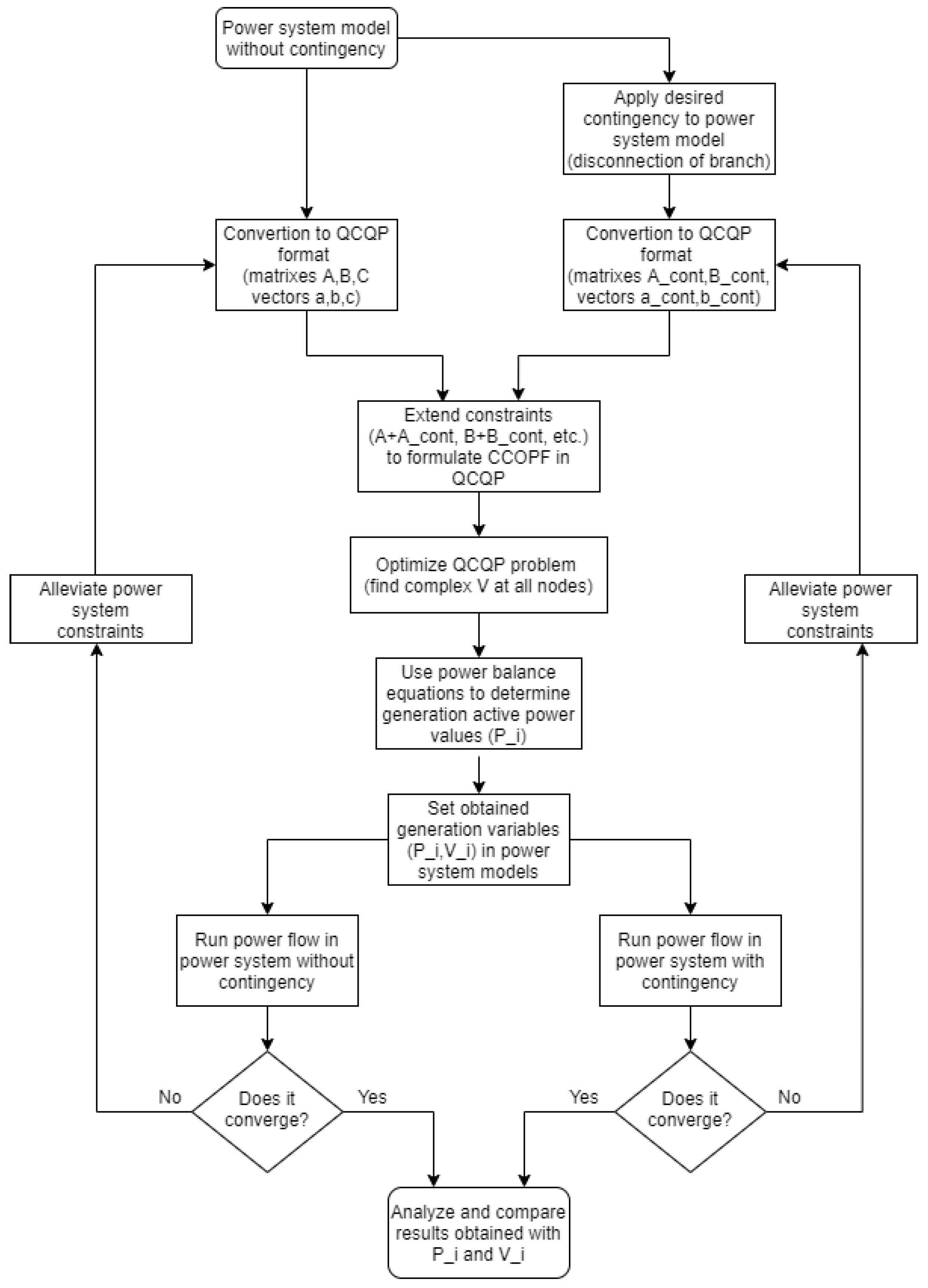
As observed, this OPF representation can be easily manipulated to add more restrictive constraints building a CCOPF formulation using the QCQP format, optimizing the objective function and complying with both pre-contingency and post-contingency constraints of the selected contingency cases. The methodology is explained next and shown in the flowchart of Figure 2:
- A contingency in the test network is carried out (e.g., disconnection of specific branch)
- The equivalent QCQP instance of the previous edited (under contingency) power system is calculated ().
- The original power system (without contingencies) is transformed into a QCQP instance.
- In the QCQP instance of the original power system (), equality constraints matrix and vector of the power system under contingency () are indexed to the original ones ().
- This final system is optimized and, due to its constraints, the resulting dispatch allows the system to work with their variables between limits in both cases: with and without contingencies.
This methodology takes advantage of the QCQP instance formulation to determine different constraint matrices and vectors, according to the power system topology, which can be indexed in a bigger QCQP instance to solve an OPF meeting with the constraints prior to and after a change in the power system topology. This is a CCOPF formulation, considering a contingency (or the consequence of a contingency) as a change in the topology of the network.
3.2. Optimal Power Flow of Extended Network
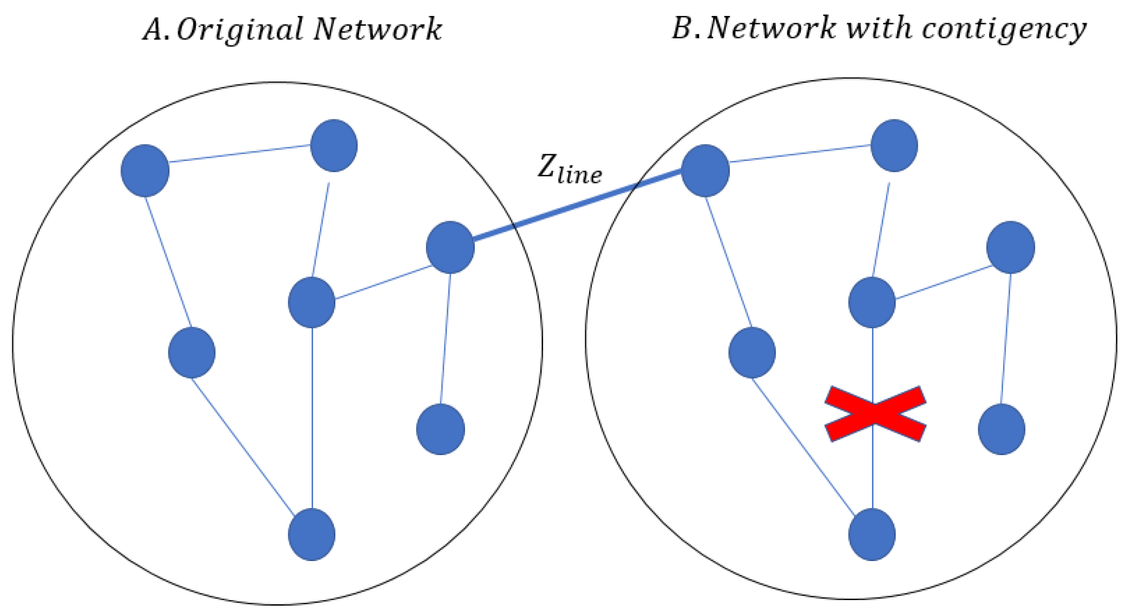
One way to evaluate the generation dispatch under CCOPF can be explored by using traditional OPF formulations. For this purpose, the network of study is cloned and both power networks are connected through a high impedance transmission line that prevents the pair of networks to exchange power between them. The from and to nodes of this new line have to be chosen iteratively, ensuring no power flow across the transmission line. As shown in Figure 3, the duplicated network is subjected to a contingency, while the original system remains intact. This model allows to force different corrective CCOPF solutions by adjusting the constant terms in the inequality constraints of the stressed network, which can be done easily. The solution will be obtained through the commonly known interior point method of the traditional OPF.
This forced solution can also be extended to comply with more restrictive constraints not necessarily included in the original CCOPF problem. As an example, a constraint that forces the simulation to find a solution in which voltage magnitudes at all nodes is kept unchanged prior to () and after () the contingency will be added to the extended OPF formulation, by defining the constraint as
In order to find the power dispatch that meets the same voltage magnitudes after the contingency occurs, the generation cost coefficients in the duplicated network are suppressed, in that way, the stressed network will only focus on replicating the conditions prior to the contingency (which are obtained from the minimization of its operational cost) without considering the economical impact, avoiding possible divergences in the simulation. This condition is required for small industrial parks with small size power networks [15,16,27].
When optimizing this new extended network by using the traditional OPF solvers, two power dispatches are obtained, both ensuring same voltages at all nodes in pre- and post-contingency scenarios. In order to implement this change in the power dispatches, generation sources should have low levels of inertia, which may define this as a corrective CCOPF strategy, useful for power networks that do not allow to have any variation in the voltage magnitudes in steady state after the contingency occurs.
4. Results and Comparison
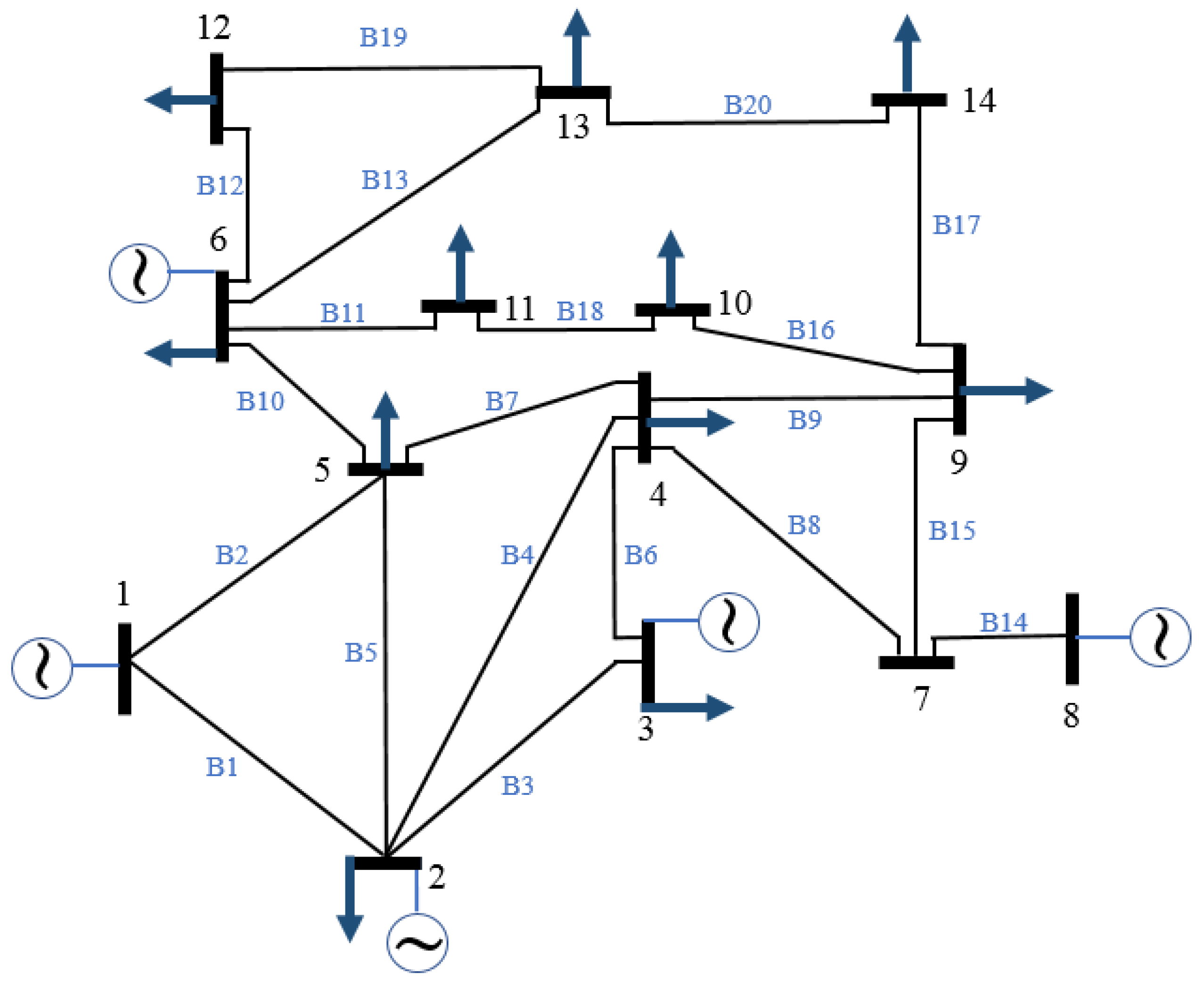
Both defined approaches are tested on the IEEE 14 bus test case network of Figure 4, composed of 14 nodes, 20 branches, and five generator agents; all of them traditional generators (all coefficients are positive). In order to compare results, the linear power operation cost function (13) is used and contingencies (disconnection of branches) in branches 5, 10, and 16 are evaluated. Bus, generator, and branch test case data is summed in Table A1, Table A2 and Table A3 located in Appendix A.
4.1. Quadratically Constrained Quadratic Programming Formulation
4.1.1. Thermal Generation Only
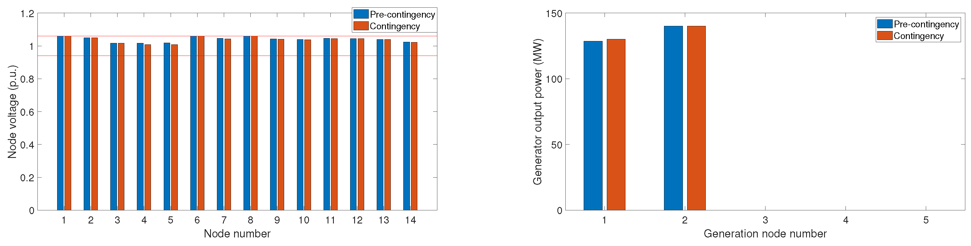
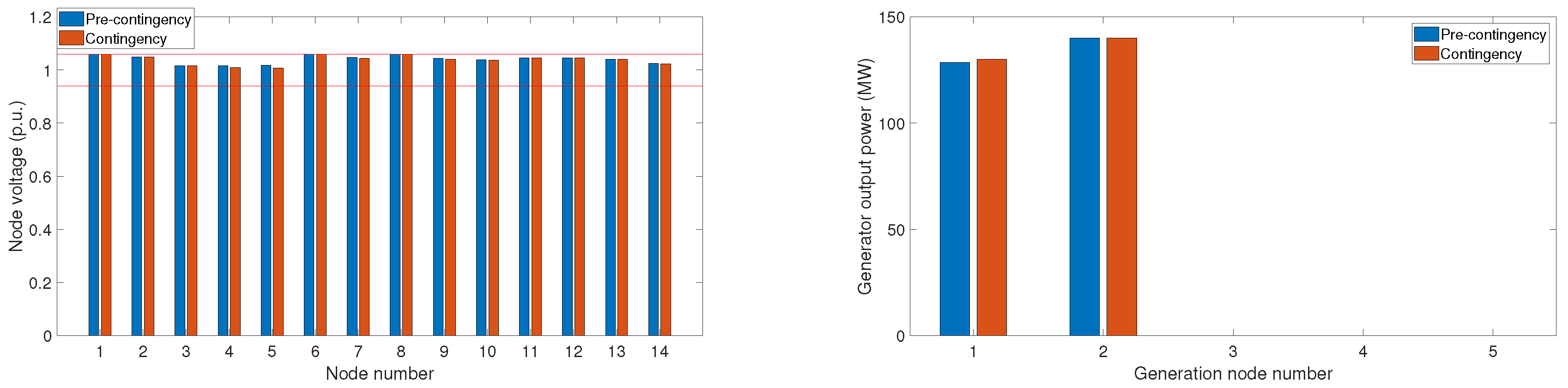
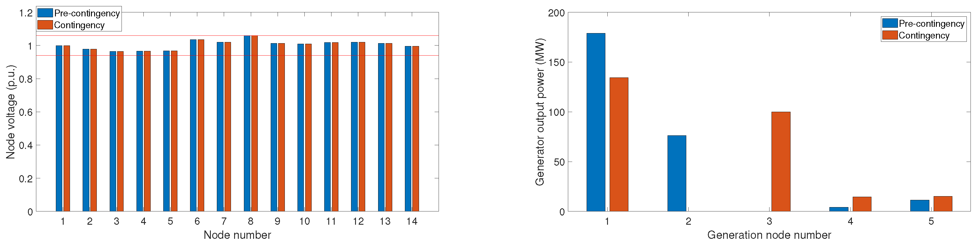
In this formulation, equality and inequality constraints of the system without and with contingency are mixed in an unique set of constraints and solved in the QCQP format. The resulting voltages and power dispatch obtained in the solution are assigned to the original power network without and with the applied contingency. Three different contingencies are simulated by disconnecting branches 5, 10, and 16. After assigning generators setpoints (P and V), a power flow takes place until convergence is achieved in the network. Figure 5, Figure 6 and Figure 7 show the final voltages and power dispatches for both scenarios. It can be observed in these three figures that the power setpoints for the generators are closely maintained after the contingency occurs. Only an increasing change is perceived in the case of generator 1, which is the slack node of the system, this suggests that branch disconnection increases active power losses in the network, which are compensated by the slack generator of the system. On the other hand, few voltage regulations are observed. In the three contingencies analyzed buses 4 and 5 present changes. When branch 5 and 16 are disconnected, voltage magnitudes at buses 4, 5, and 14 decrease, while, when branches 10 gets disconnected, the magnitude at buses 4 and 5 increases as well as in buses 10, 13, and 14.
It can be observed that the QCQP formulation only dispatches generators 1 and 2 at its maximum power in both pre- and post-contingency scenarios, so no big adjustment has to be made in the generation dispatch regulation. Voltage magnitudes at all nodes are not the same prior to and after contingency, due to the slight regulation of power of the generation agents, which presented a maximum change in power of in generator 1 after branch 10 was disconnected. Maximum values of voltage regulation obtained were of at node 5 after branch 5 and branch 16 were disconnected. It is important to note that even if voltages at all nodes have changes, in both scenarios voltage magnitudes are between specified bounds.
4.1.2. Thermal and Photovoltaic Generation
Photovoltaic generation with battery storage is also included in the QCQP formulation by changing the coefficient of Equation (13). Generator 4, located at node 6, is selected to represent a photovoltaic generator with battery storage. Generator data is the same as presented in bus number 6 of Table A2 in Appendix A, with the only difference of having its coefficient sign changed to negative. Figure 8, Figure 9 and Figure 10 show the results obtained for pre- and post-contingency cases after fixing generation setpoints obtained in the QCQP formulation.
Test results show the behavior observed for the case with traditional generation in both strategies. The same power dispatch is practically kept for pre and post contingency scenarios, with a maximum percentage change of experienced at generator 1 after branch 10 is disconnected. In some nodes, there is a change in the voltage magnitude, some cases greater after the contingency, some others lower. The maximum regulation observed was of at node 10 after branch 10 was disconnected.
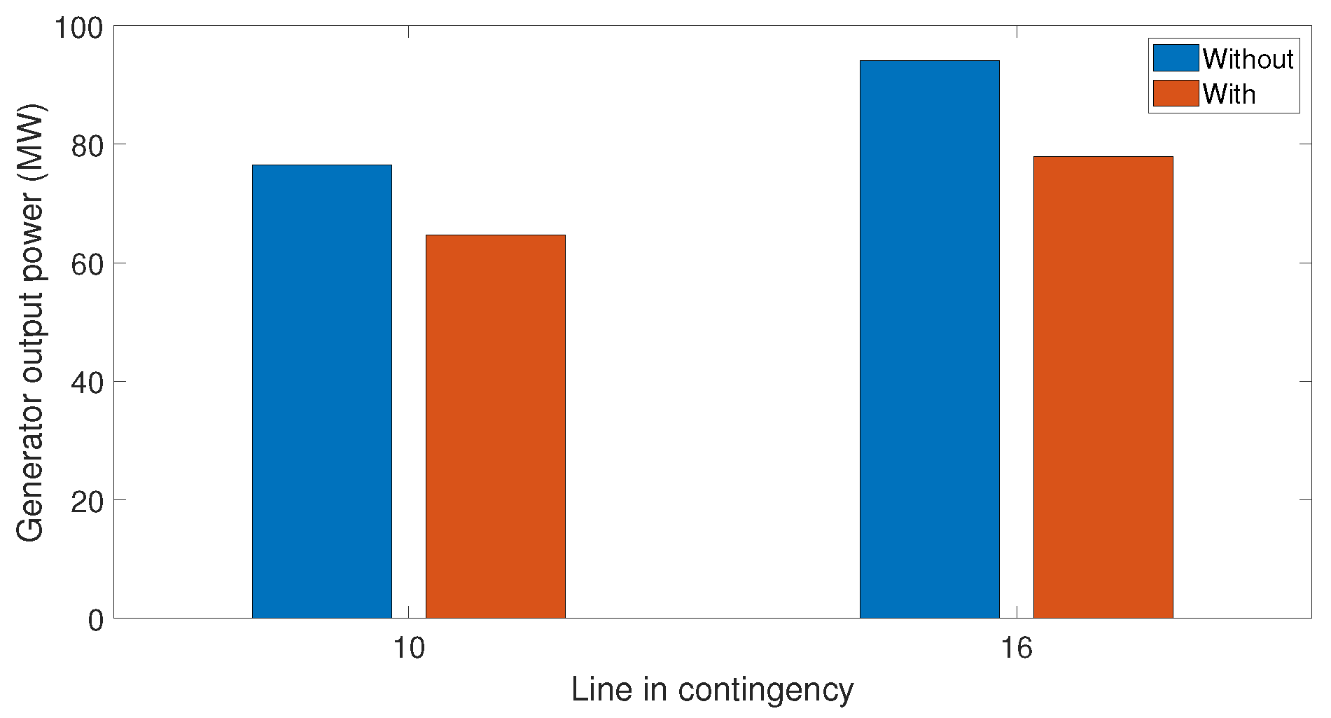
When including PV generation, the QCQP strategy tends to dispatch it as much as possible, assuming the resource is available. In order to check the sensitivity of this behavior when branches connecting the generator have more restrictive limits, power flow through transmission lines connecting the renewable PV generation source is restricted to 25 MVA. This was decided because the maximum power output of generator 4 is 100 MVA and there are 4 transmission lines connected to it. A comparison of the power dispatched by the PV generator without and with this loadability restriction after disconnection of branches 5, 10, and 16 is shown in Figure 11.
As observed, there is a small reduction in the dispatched power; however, the amount dispatched is still considerably high for the generator, meaning that the strategy is in a certain way, sensitive to these loadability constraints when dispatching renewable generation. Strict power flow restriction changes and settings in the adjacent branches of PV generator after contingency will reduce its amount of active power dispatched, which entails to a more expensive operational cost of the system than without including strict loadability constraints. The changes observed in the dispatch may be due to a relaxation in the power flow of some of the adjacent connecting lines of the PV generator. It is probable that the amount dispatched by the the PV generator is not equally distributed in their 4 connecting lines, and as consequence, some of the lines are loaded to more than 25 MVA without having loadability restrictions. Now, when restrictions are applied, lines overloaded are regulated adjusting the power dispatched by the PV generator and the power difference is supported by the thermal generators, while meeting all the constraints.
4.2. Optimal Power Flow of the Extended Network
4.2.1. Thermal Generation Only
In this case, the system was duplicated and both networks were interconnected through a transmission line from the last node of the original system to the last node of the duplicated system. Resistance, inductance, and susceptance of the new line were adjusted in order to avoid power flow between the two networks. The choice of nodes connecting the systems is based on the amount of power flow obtained after running an OPF when interconnecting both networks without contingencies. Iteratively, power flow through the connecting transmission line is evaluated and those lines that present power flows of less than 1 MVA are considered as a good starting point for its implementation, considering that power flows of less than 0.5 MVA were found to not interfere in the power flow operation of both networks, and that changes in the new branch could reduce even more its initial power flow, i.e., increasing the impedance of the branch by adjusting its electrical parameters.
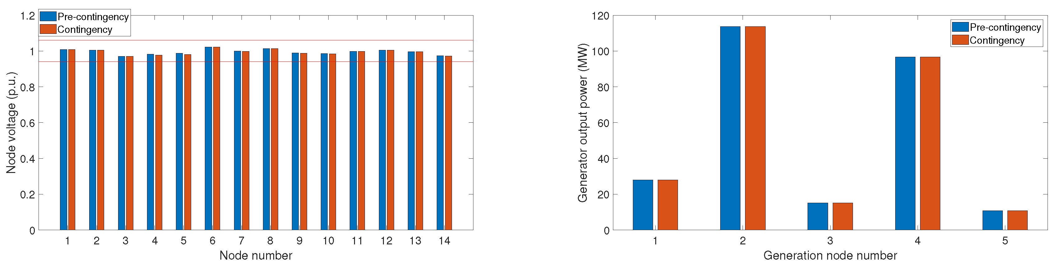
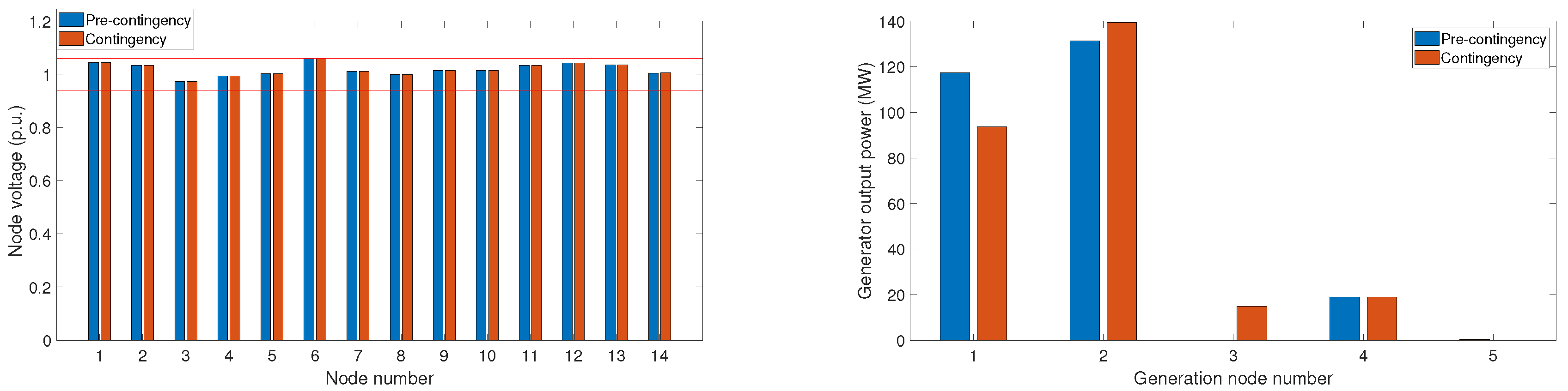
The results obtained show that all original system nodes have the same voltage than those of the duplicated system, complying with constraint (19). Due to the change in topology when the contigency is applied, a change in power dispatch is needed in order to keep the same voltage magnitudes in pre-contingency and contingency scenarios; these voltages are also within limits at all nodes. For this reason, the power dispatch may be regulated when the contingency occurs and the operation cost may change as well. Figure 12, Figure 13 and Figure 14 show the obtained voltages and power dispatches for contingencies in lines 5, 10, and 16 compared to those when the system works without any contingency.
4.2.2. Thermal and Photovoltaic Generation
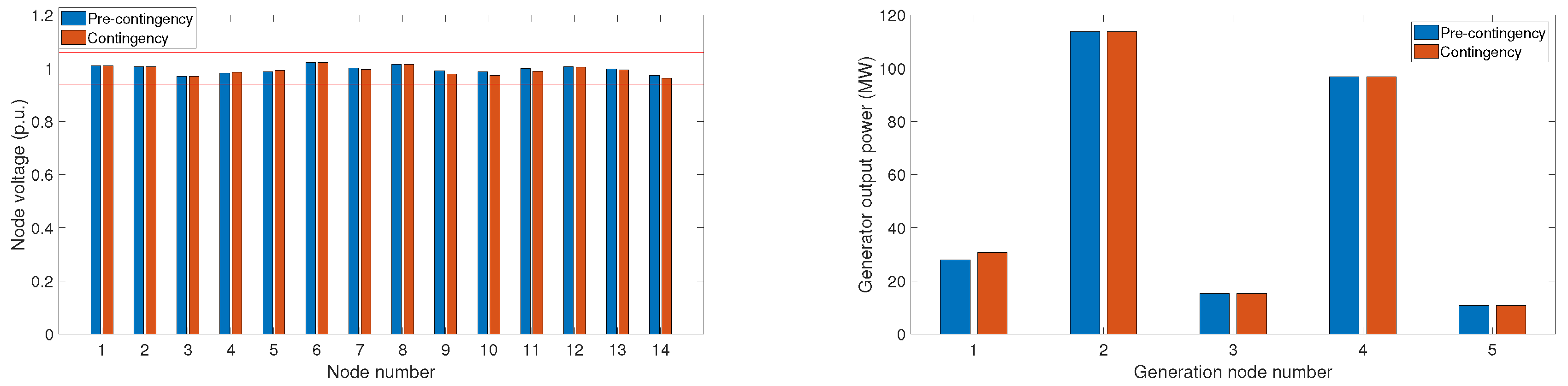
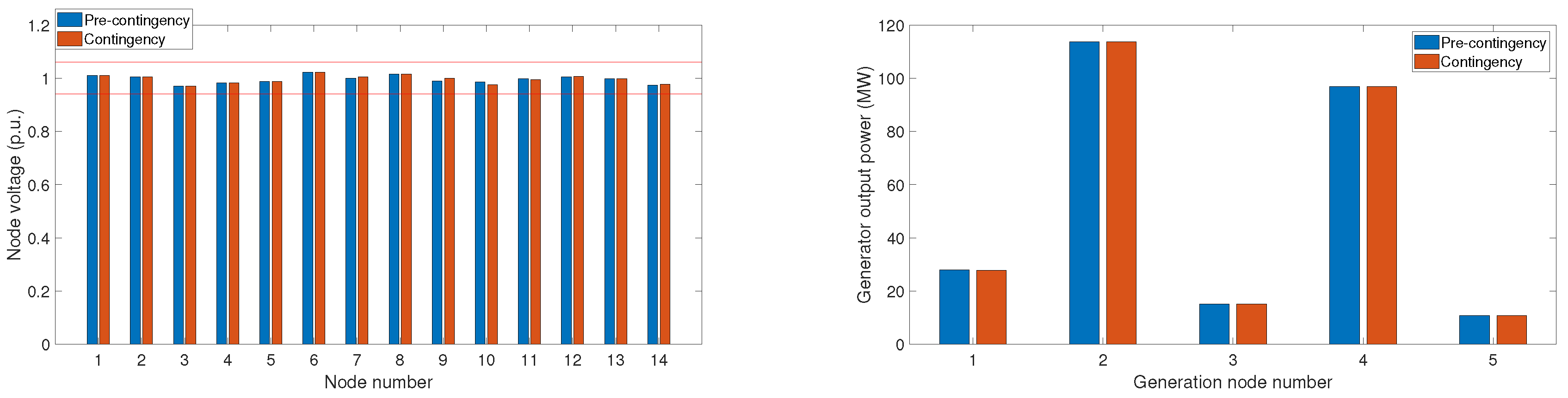
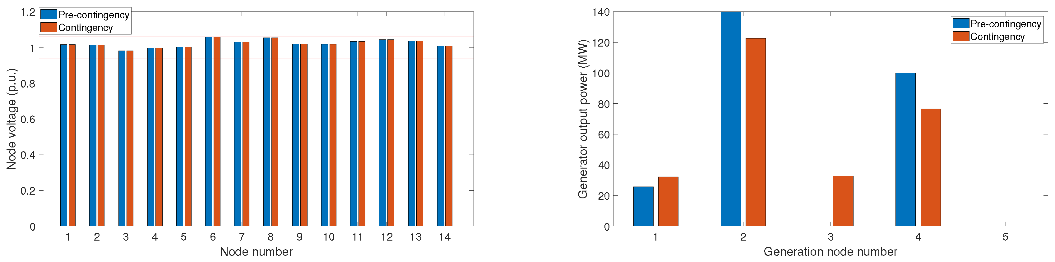
The strategy is now evaluated including one photovoltaic generator at node 6. To do so, the sign of the coefficient of generator 4 is changed to negative. Figure 15, Figure 16 and Figure 17 show the obtained power dispatch and voltages at all nodes following the proposed strategy. It can be observed that in all branch disconnections, voltage magnitudes are kept equal to the pre-contingency condition after their disconnection occurs. To achieve this condition, regulation in generation active power dispatched must take place. After disconnection of branches 5 and 10, the generator at node 3, which is a traditional type generator, needs to be started in order to keep voltage regulation of in all nodes comparing with the pre-contingency state. Starting the generator alleviates the voltage regulation that could appear in nodes 2 and 4 and their adjacent nodes when the active power of these machines is not reduced. Generator 4, which is the PV generator with battery storage, is always dispatched in all situations, but not dispatched at its maximum in some cases. This may be due to an impossibility to meet the condition of keeping same node voltages prior to and after the contingency.
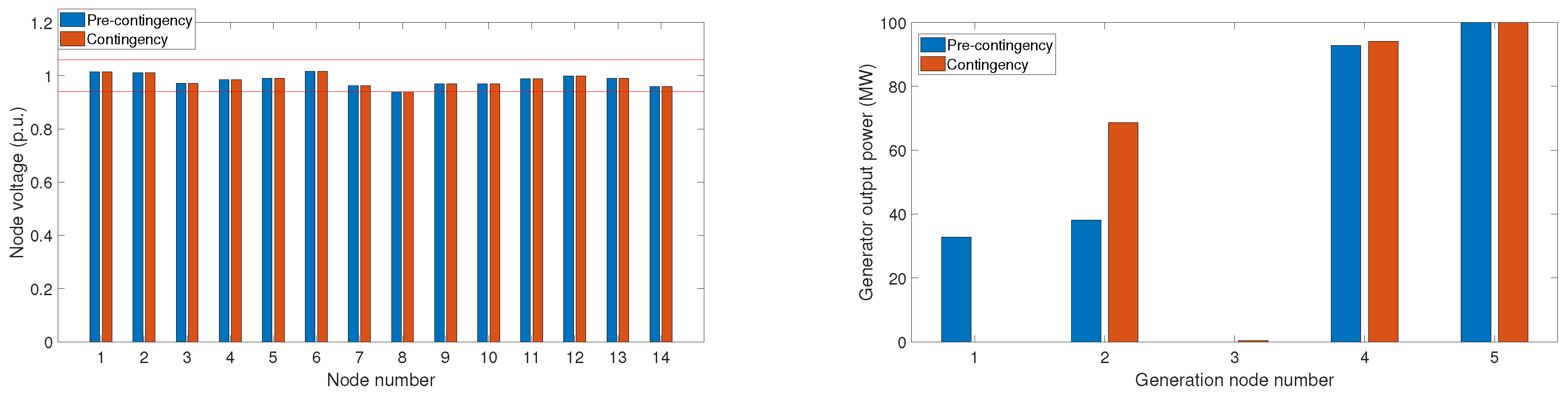
In order to compare the sensitivity of the PV power dispatch obtained when including strict power flow constraints in branches connecting the PV generator within this extended OPF strategy, critical loadability limits (25 MVA) for the adjacent transmission lines of generator 4 are implemented and a comparison of the different dispatches with and without this constraint for disconnection of branches 10 and 16 is presented in Figure 18. Disconnection of branch 5 is not analyzed because, even though the strategy finds a solution when all branches are connected (having loadability limits or without having them), when loadability limits are applied and branch 5 is disconnected, the system did not converge. This is suspected to occur due to an impossibility of keeping voltage magnitudes equal after the disconnection of branch 5 without the PV generator loading one of its near connecting branches in more than 25 MVA. As shown in Figure 15, the dispatch of the PV generator located in node 4 without loadability limits is the nominal capacity of the generator (100 MW) and its dispatch is the same prior and after the contingency occurs. As power flow limits of the branches connected to the generator are restricted in this case, it is possible that after contingency, the generator could not be dispatched to its nominal capacity without overloading one of its connecting branches and as a consequence, some nodes may have regulation in their voltages, which prevents the system to meet the constraint of Equation (19).
In this case, the change of power dispatch is greater than the obtained in the QCQP strategy, which presumably might be related to meeting the same voltage prior to and after the contingency condition. This is a more restrictive problem than the one formulated in the QCQP strategy, which does have some voltage regulation in their results. The changes present in the dispatch of PV generation for the extended OPF strategy are mainly due to trying to obtain the same voltage magnitude in all nodes respecting branch power flow limits which could limit the amount of power dispatched by the PV generator, and as consequence, changes the voltage magnitude of adjacent nodes. The results obtained exposes a high sensitivity of this strategy when changing loadability limits, as for one of the contingencies, the system did not even converge after the disconnection of the branch and the maximum variation of dispatched power obtained for the other contingencies is of 17% based in the original power dispatched value, while in the QCQP strategy, the maximum percentage change obtained was of near to 6%.
Sensitivity in both strategies is understand in this work as the measure of change of the behavior in the power dispatched by the PV generator implemented, when considering more severe restrictions after the contingency occurs. In the case of the renewable dispatched power, one could expect it to be dispatched at its maximum in order to reduce operational cost; however, presence of high sensitivity shows that operational cost can be highly compromised when selecting strict power flow constraints and expecting to meet all system constraints after the contingency happens.
4.3. Results Comparison
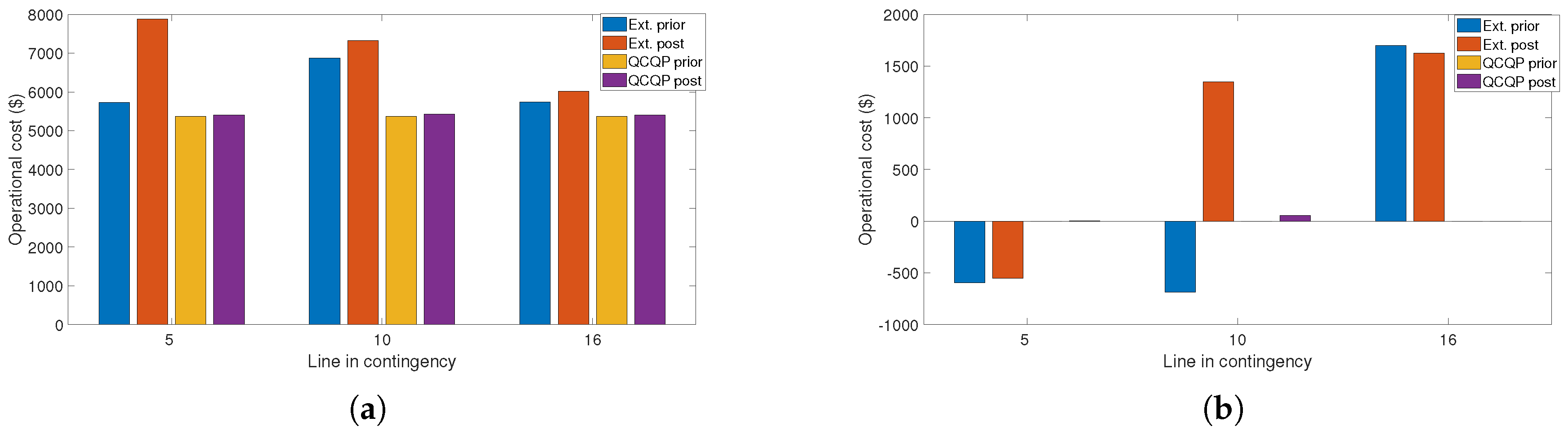
Results obtained with both approaches are not equal since the main objectives of both strategies differ. In the QCQP formulation, the generation dispatch found is supposed to be the same prior and after the contingency with the exception of the generator selected as slack. As a consequence, some voltage regulation could exist at all nodes after branch disconnection. On the other hand, in the extended OPF approach, the dispatches in all generators could change in an arbitrarily manner but the voltage magnitudes at all nodes must stay the same. This two main objectives lead to the results obtained and previously presented, where there is almost no power regulation in generation dispatches for the QCQP approach but there is presence of voltage regulation at some nodes of the system, and, in the case of the extended OPF, there is no regulation in voltage magnitudes at all nodes, but there are significant changes in the power dispatched by the generators prior and after the contingency. Even though the main focus of the two strategies vary because of the difference in their formulations and, in the case of the extended OPF strategy, the inclusion of an additional constraint, it is possible to compare the economic performance of both operational strategies from the obtained power dispatches. In Figure 19a the bar graph of operational cost for both operations (prior to and post contingency) is presented for each strategy using only thermal generation while in Figure 19b the bar graph shows the case when one PV generator with battery storage is included in the system.
The negative values obtained in the case of thermal and PV generation are due to the negative coefficient modified from the original power system structure implemented in the matpower toolbox. It also has to be noted that no coefficients are implemented in the original structure, as shown in Table A2 in Appendix A, meaning that all linear operation cost functions (13) have their intercept in the origin and by no means could represent a real operational cost for any real generation agent. However, the coefficients allow us to evaluate the operation of the system economically by only taking into account each generated power unit in all generators and, although this cost coefficient magnitudes are far from being what could be found in a real case, they help us to normalize the study conditions and to compare results of different operational strategies under the same reference frame.
Comparisons of all dispatches obtained for every contingency applied in the system without critical loadability limits are found in Figure 19. It is observed in Figure 19a that, when the system has thermal generation only, the extended OPF strategy presents a more expensive operational cost than that of the QCQP strategy prior to and after each contingency occurs. When adding PV generation in the system (Figure 19b), it is observed as well that when applying the disconnection of branch number 16, the operational cost is greater than the cost of the QCQP strategy, for both prior-post scenarios, which leads us to conclude that the behavior of the extended OPF strategy is more focused on finding dispatches that are able to meet with all constraints established (including same voltage magnitudes) in both power networks rather than an actual minimization of the operational cost in the execution of the strategy. The extended OPF strategy is proved to be more expensive than the QCQP in all disconnections performed when having thermal generation only. However, when adding one PV generator with storage, the operational cost found prior to and after disconnecting branch 5 and prior to disconnection of branch 10 had negative values which were less than the operational costs for the same cases with PV generation in the QCQP formulation, these cheaper operational costs in the extended OPF strategy are considered exceptions, as the majority of the operational costs found for the extended OPF strategy were found to be greater than the costs obtained with QCQP.
On the other hand, the QCQP results obtained (Figure 5, Figure 6, Figure 7, Figure 8, Figure 9 and Figure 10) can be considered stiff with low variation in the power dispatch and voltage magnitudes for both thermal and thermal + PV generation scenarios in the three contingencies analyzed. Moreover, the operational costs results were lower than those of the extended OPF strategy for the majority of cases prior to and after the contingency (Figure 19a,b). Even though each contingency was analyzed individually, the power dispatch results in the three cases are similar. As the QCQP strategy can be easily extended to more than one contingency, it is expected that the power dispatch result of a more complete format with more than one contingency will be similar if not equal to the obtained dispatches for each contingency.
For both strategies, execution times were compared within this test system. The maximum difference in execution times observed was of approximately 750 ms in the contingency at branch 5 with thermal and PV generation. The QCQP strategy presented the slowest execution times when the system had thermal and PV generation. Simulations in both strategies ran in less than 700 ms for the cases with thermal generation only. Even though it may appear that the extended OPF strategy would be better based on its execution time, it is reminded that the result obtained with this strategy is focused on a corrective CCOPF perspective, while the QCQP strategy presents a result focused on a preventive CCOPF perspective. Execution times for all cases simulated are presented in Table 2.
Simulations in systems with more buses coincided that the QCQP strategy was much slower than the extended OPF; however, as the result of the QCQP strategy focuses on finding a preventive power dispatch for the CCOPF problem, which is supposed to remain the same after the contingencies occur. Execution time is not as critical as in the extended OPF strategy which has a corrective CCOPF perspective, where finding a power dispatch solution and making corrective actions are to be performed in a short window of time (short-term time frame analysis), this will be more challenging as systems grow in size and number of nodes due to the increase of execution time in the simulation. Selection of any methodology proposed will depend on the objectives specified by the network operator, and on the elements included in the power network with capabilities to regulate the power dispatch or voltage magnitudes in the system.
5. Conclusions
Two different operation strategies based on the CCOPF concept were presented and implemented in a power network with 14 nodes. Both strategies are developed in the matpower format and presented different results. The first one is a conception of a CCOPF problem using QCQP instances equivalent to those of an optimal power flow. The QCQP instance is modified to include contingency constraints that allow the power network to have the same power dispatch before and after a line disconnection stresses the power network. Separately, three different lines were taken out of the system and the performance of the QCQP programming strategy was evaluated through the voltage magnitudes of each node in the system prior and after the contingency happened. A maximum percentage change in the power dispatch of and in the voltage magnitude of was obtained for the QCQP strategy in a power network composed of only thermal generators, while in the case of thermal generation and one controllable photovoltaic generator with battery storage, maximum percentages of change in power dispatch and voltage of 10% and 1.3%, respectively, were obtained. It was also determined that if a PV generator is connected to the system, the strategy searches to dispatch it as much as possible. The QCQP strategy presents small sensitivity in its results when changes in the loadability constraints of lines adjacent to the PV generator are stricter.
The second strategy in this work is defined as a CCOPF corrective strategy that aims to have the same voltage magnitudes (no regulation) in steady state of a power system that is being affected by a contingency in one of its branches. As before, three different contingencies were applied to the power network when having only thermal generation and thermal generation plus one controllable PV generator with battery storage. The results obtained show that in all cases, the voltage magnitudes at all nodes are kept the same but the dispatched power prior to and after the contingency occurs can differ completely in some generators, even having to stop the operation of one of them and re-dispatch its previous power between the other machines. Furthermore, it was observed that this strategy is highly sensitive to changes of loadability constraints in transmission lines connected to the simulated controllable PV generator with energy storage. When loadability constraints changed to be stricter ones in the adjacent lines of the PV generator with battery storage, the solution to the CCOPF after disconnection of branch 5 was performed did not converge and it was impossible to find a power dispatch meeting the constraints. The extended OPF strategy is proposed to be implemented in small power systems that require fixed voltage values for its operation, and where the generators connected to these power systems have small inertia values in order to change their dispatched power rapidly after the contingency is detected.
Both methodologies can be extended to include more than one contingency. The use of these methodologies is encouraged to be implemented in power flow software tools, specially, the extended OPF approach for CCCOPF, which does not need any particular additional solver to be executed; however, this strategy does need to include the new constraint proposed in order to keep all node voltages equal after a branch disconnection. This strategy could be implemented in a more practical way after a less empirical methodology for the creation of an interconnection branch between power systems with and without contingency is established. On the other hand, the QCQP strategy does need to account with a convertion function that takes the original system structured in the power system software and transform it into a QCQP problem as discussed in Section 3 of this paper. An additional optimization solver is needed to obtain the accurate dispatch before running a power flow in the software, which makes this implementation more complicated but still promising.
Author Contributions
Conceptualization, L.M.L., A.S.B., and S.R.; methodology, L.M.L., S.R. and A.S.B.; validation, L.M.L. and A.S.B.; formal analysis, A.S.B., S.R., and L.M.L.; investigation, L.M.L., A.S.B. and A.S.; resources, L.M.L. and A.S.B.; data curation, L.M.L.; writing—original draft preparation, L.M.L., S.R. and A.S.B.; writing—review and editing, L.M.L., S.R. and A.S.B.; visualization, L.M.L., A.S.B. and S.R.; funding acquisition and supervision, A.S.B., and S.R. and A.S. All authors have read and agreed to the published version of the manuscript.
Funding
This research received no external funding.
Acknowledgments
This work was supported by Universidad Nacional de Colombia. Additionally, the authors would like to give thanks to: RED IBEROAMERICANA PARA EL DESARROLLO Y LA INTEGRACION DE PEQUENHOS GENERADORES EOLICOS (MICRO-EOLO) for their support.
Conflicts of Interest
The authors declare no conflicts of interest.
Appendix A

Table A1.
IEEE 14-bus data used.
| Bus Number | [MW] | [MW] | [p.u.] | [p.u.] |
|---|---|---|---|---|
| 1 | 0 | 0 | 1.06 | 0.94 |
| 2 | 21.7 | 12.7 | 1.06 | 0.94 |
| 3 | 94.2 | 19 | 1.06 | 0.94 |
| 4 | 47.8 | −3.9 | 1.06 | 0.94 |
| 5 | 7.6 | 1.6 | 1.06 | 0.94 |
| 6 | 11.2 | 7.5 | 1.06 | 0.94 |
| 7 | 0 | 0 | 1.06 | 0.94 |
| 8 | 0 | 0 | 1.06 | 0.94 |
| 9 | 29.5 | 16.6 | 1.06 | 0.94 |
| 10 | 9 | 5.8 | 1.06 | 0.94 |
| 11 | 3.5 | 1.8 | 1.06 | 0.94 |
| 12 | 6.1 | 1.6 | 1.06 | 0.94 |
| 13 | 13.5 | 5.8 | 1.06 | 0.94 |
| 14 | 14.9 | 5 | 1.06 | 0.94 |
Table A2.
IEEE 14-generator data used.
| Bus Number | [MVAr] | [MVAr] | [MW] | [MW] | [] | [] | [$] |
|---|---|---|---|---|---|---|---|
| 1 | 10 | 0 | 332.4 | 0 | 0 | 20 | 0 |
| 2 | 50 | −40 | 140 | 0 | 0 | 20 | 0 |
| 3 | 40 | 0 | 100 | 0 | 0 | 40 | 0 |
| 6 | 24 | −6 | 100 | 0 | 0 | 40 | 0 |
| 8 | 24 | −6 | 100 | 0 | 0 | 40 | 0 |
Table A3.
IEEE 14-branch data used.
| Branch Number | ||
|---|---|---|
| 1 | 1 | 2 |
| 2 | 1 | 5 |
| 3 | 2 | 3 |
| 4 | 2 | 4 |
| 5 | 2 | 5 |
| 6 | 3 | 4 |
| 7 | 4 | 5 |
| 8 | 4 | 7 |
| 9 | 4 | 9 |
| 10 | 5 | 6 |
| 11 | 6 | 11 |
| 12 | 6 | 12 |
| 13 | 6 | 13 |
| 14 | 7 | 8 |
| 15 | 7 | 9 |
| 16 | 9 | 10 |
| 17 | 9 | 14 |
| 18 | 10 | 11 |
| 19 | 12 | 13 |
| 20 | 13 | 14 |
References
- Capitanescu, F.; Ramos, J.M.; Panciatici, P.; Kirschen, D.; Marcolini, A.M.; Platbrood, L.; Wehenkel, L. State of the art, challenges, and future trends in security constrained optimal power flow. Electr. Power Syst. Res. 2019, 81, 1731–1741. [Google Scholar] [CrossRef] [Green Version]
- Tang, L.; Sun, W. An automated transient stability constrained optimal power flow based on trajectory sensitivity analysis. IEEE Trans. Power Syst. 2016, 32, 590–599. [Google Scholar] [CrossRef]
- Nguyen-Duc, H.; Tran-Hoai, L.; Ngoc, D.V. A novel approach to solve transient stability constrained optimal power flow problems. Turkish J. Electr. Eng. Comput. Sci. 2017, 25, 4696–4705. [Google Scholar] [CrossRef]
- Hinojosa, V.H. An improved corrective security constrained OPF for meshed AC/DC grids with multi-terminal VSC-HVDC. Energies 2020, 13, 516. [Google Scholar] [CrossRef] [Green Version]
- Stott, B.; Alsaç, O. Optimal power flow: Basic requirements for real-life problems and their solutions. In Proceedings of the SEPOPE XII Symposium, Rio de Janeiro, Brazil, 20–23 May 2012. [Google Scholar]
- Gunda, J.; Djokic, S.; Langella, R.; Testa, A. On convergence of conventional and meta-heuristic methods for security-constrained OPF analysis. In Proceedings of the 31st Annual ACM Symposium on Applied Computing, Pisa, Italy, 3–6 April 2016; pp. 109–111. [Google Scholar]
- Karbalaei, F.; Shahbazi, H.; Mahdavi, M. A new method for solving preventive security-constrained optimal power flow based on linear network compression. Int. J. Electr. Power Energy Syst. 2018, 96, 23–29. [Google Scholar] [CrossRef]
- Cao, J.; Du, W.; Wang, H.F. An improved corrective security constrained OPF for meshed AC/DC grids with multi-terminal VSC-HVDC. IEEE Trans. Power Syst. 2015, 31, 485–495. [Google Scholar] [CrossRef]
- Capitanescu, F.; Wehenkel, L. A new iterative approach to the corrective security-constrained optimal power flow problem. IEEE Trans. Power Syst. 2008, 23, 1533–1541. [Google Scholar] [CrossRef] [Green Version]
- Gunda, J.; Djokic, S.; Langella, R.; Testa, A. Comparison of conventional and meta-heuristic methods for security-constrained OPF analysis. In Proceedings of the AEIT International Annual Conference (AEIT), Naples, Italy, 14–16 October 2015; pp. 1–6. [Google Scholar]
- Fang, D.; Gunda, J.; Djokic, S.Z.; Vaccaro, A. Security-and time-constrained OPF applications. In Proceedings of the IEEE Manchester PowerTech, Manchester, UK, 18–22 June 2017; pp. 1–6. [Google Scholar]
- Kaur, M.; Dixit, A. Newton’s Method approach for Security Constrained OPF using TCSC. In Proceedings of the IEEE 1st International Conference on Power Electronics, Intelligent Control and Energy Systems (ICPEICES), Delhi, India, 4–6 July 2016; pp. 1–5. [Google Scholar]
- Wu, X.; Zhou, Z.; Liu, G.; Qi, W.; Xie, Z. Preventive security-constrained optimal power flow considering UPFC control modes. Energies 2017, 10, 1199. [Google Scholar] [CrossRef] [Green Version]
- Nycander, E.; Söder, L. Comparison of stochastic and deterministic security constrained optimal power flow under varying outage probabilities. In Proceedings of the IEEE Milan PowerTech, Milan, Italy, 23–27 June 2019; pp. 1–6. [Google Scholar]
- Gao, X.; Lu, X.; Chan, K.W.; Hu, J.; Xia, S.; Xu, D. Distributed Coordinated Management for Multiple Distributed Energy Resources Optimal Operation with Security Constrains. In Proceedings of the IEEE Power and Energy Society Innovative Smart Grid Technologies Conference (ISGT), Washington, DC, USA, 18–21 February 2019; pp. 1–5. [Google Scholar]
- Cao, J.; Liu, Y.; Ge, Y.; Cai, H.; Zhou, B.W. Enhanced corrective security constrained OPF with hybrid energy storage systems. In Proceedings of the UKACC 11th International Conference on Control (CONTROL) IEEE, Belfast, UK, 31 August–2 September 2016; pp. 1–7. [Google Scholar]
- Nasr, M.A.; Nikkhah, S.; Gharehpetian, G.B.; Nasr-Azadani, E.; Hosseinian, S.H. A multi-objective voltage stability constrained energy management system for isolated microgrids. Int. J. Electr. Power Energy Syst. 2020, 117, 105646. [Google Scholar] [CrossRef]
- Alzalg, B.; Anghel, C.; Gan, W.; Huang, Q.; Rahman, M.; Shum, A.; Wu, C.W. Contingency constrained optimal power flow solutions in complex network power grids. In Proceedings of the IEEE International Symposium on Circuits and Systems, Seoul, Korea, 20–23 May 2012; pp. 1636–1639. [Google Scholar]
- Wang, Q.; McCalley, J.D.; Zheng, T.; Litvinov, E. A computational strategy to solve preventive risk-based security-constrained OPF. IEEE Trans. Power Syst. 2012, 28, 1666–1675. [Google Scholar] [CrossRef]
- Van Acker, T.; Van Hertem, D. Linear representation of preventive and corrective actions in OPF models. In Proceedings of the Young Researchers Symposium, Eindhoven, The Netherland, 12–13 May 2016. [Google Scholar]
- Zimmerman, R.D.; Murillo-Sánchez, C.E.; Thomas, R.J. MATPOWER: Steady-State Operations, Planning and Analysis Tools for Power Systems Research and Education. IEEE Trans. Power Syst. 2011, 26, 12–19. [Google Scholar] [CrossRef] [Green Version]
- Zimmerman, R.D.; Murillo-Sánchez, C.E. Matpower User’s Manual, Version 7.0. 2019. Available online: https://matpower.org/docs/MATPOWER-manual-7.0.pdf (accessed on 2 May 2020).
- Bernal, J.; Neira, J.; Rivera, S. Mathematical Uncertainty Cost Functions for Controllable Photo-Voltaic Generators considering Uniform Distributions. WSEAS Trans. Math. 2019, 18, 137–142. [Google Scholar]
- Gaing, Z.; Lin, C. Contingency-Constrained Optimal Power Flow Using Simplex-Based Chaotic-PSO Algorithm. In Applied Computational Intelligence and Soft Computing; Hindawi Publishing Corporation: London, UK, 2011; p. 13. [Google Scholar]
- Low, S.H. Convex relaxation of optimal power flow—Part I: Formulations and equivalence. IEEE Trans. Control Netw. Syst. 2014, 1, 15–27. [Google Scholar] [CrossRef] [Green Version]
- Josz, C.; Fliscounakis, S.; Maeght, J.; Panciatici, P. AC Power Flow Data in MATPOWER and QCQP Format: ITesla, RTE Snapshots, and PEGASE. arXiv 2016, arXiv:1603.01533. [Google Scholar]
- Vargas, A.; Saavedra, O.; Samper, M.; Rivera, S.; Rodriguez, R. Latin American Energy Markets: Investment Opportunities in Nonconventional Renewables. IEEE Power Energy Mag. 2011, 14, 38–47. [Google Scholar] [CrossRef]
Figure 1.
Interpretation of the CCOPF problem in a hypothetical network in steady state.

Figure 2.
Flowchart of CCOPF formulation using the QCQP methodology.

Figure 3.
Topology approach to find the CCOPF through traditional OPF formulations.

Figure 4.
IEEE 14 bus test system () diagram indicating generators and loads positions as well as branches with their numeration.
Figure 4.
IEEE 14 bus test system () diagram indicating generators and loads positions as well as branches with their numeration.

Figure 5.
Voltage and power dispatched implementing the QCQP results in a power flow of the network prior to and after contingency of branch 5 (generation nodes are, respectively, 1, 2, 3, 6, and 8).
Figure 5.
Voltage and power dispatched implementing the QCQP results in a power flow of the network prior to and after contingency of branch 5 (generation nodes are, respectively, 1, 2, 3, 6, and 8).

Figure 6.
Voltage and power dispatched implementing the QCQP results in a power flow of the network prior to and after contingency of branch 10 (generation nodes are, respectively, 1, 2, 3, 6, and 8).
Figure 6.
Voltage and power dispatched implementing the QCQP results in a power flow of the network prior to and after contingency of branch 10 (generation nodes are, respectively, 1, 2, 3, 6, and 8).
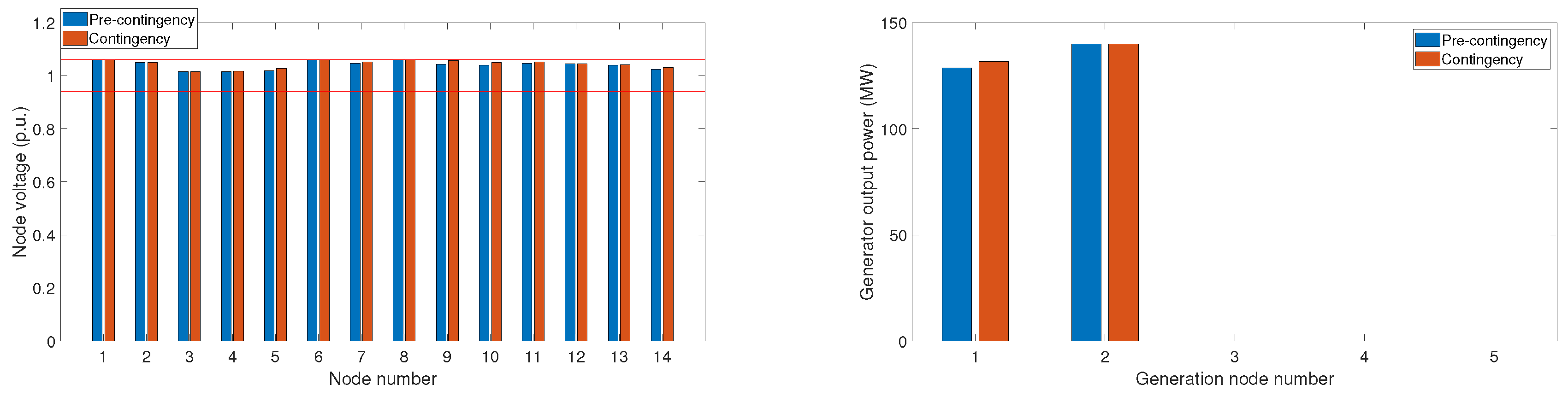
Figure 7.
Voltage and power dispatched implementing the QCQP results in a power flow of the network prior to and after contingency of branch 16 (generation nodes are, respectively, 1, 2, 3, 6, and 8).
Figure 7.
Voltage and power dispatched implementing the QCQP results in a power flow of the network prior to and after contingency of branch 16 (generation nodes are, respectively, 1, 2, 3, 6, and 8).

Figure 8.
Voltage and power dispatched implementing the QCQP results in a power flow of the network prior to and after contingency of branch 5 (generation nodes are, respectively, nodes 1, 2, 3, 6, and 8).
Figure 8.
Voltage and power dispatched implementing the QCQP results in a power flow of the network prior to and after contingency of branch 5 (generation nodes are, respectively, nodes 1, 2, 3, 6, and 8).

Figure 9.
Voltage and power dispatched implementing the QCQP results in a power flow of the network prior to and after contingency of branch 10 (generation nodes are, respectively, nodes 1, 2, 3, 6, and 8).
Figure 9.
Voltage and power dispatched implementing the QCQP results in a power flow of the network prior to and after contingency of branch 10 (generation nodes are, respectively, nodes 1, 2, 3, 6, and 8).

Figure 10.
Voltage and power dispatched implementing the QCQP results in a power flow of the network prior to and after contingency of branch 16 (generation nodes are, respectively, nodes 1, 2, 3, 6, and 8).
Figure 10.
Voltage and power dispatched implementing the QCQP results in a power flow of the network prior to and after contingency of branch 16 (generation nodes are, respectively, nodes 1, 2, 3, 6, and 8).

Figure 11.
Power dispatch of renewable generator number 4 without and with loadability restrictions for every contingency applied (disconnection of branch).
Figure 11.
Power dispatch of renewable generator number 4 without and with loadability restrictions for every contingency applied (disconnection of branch).
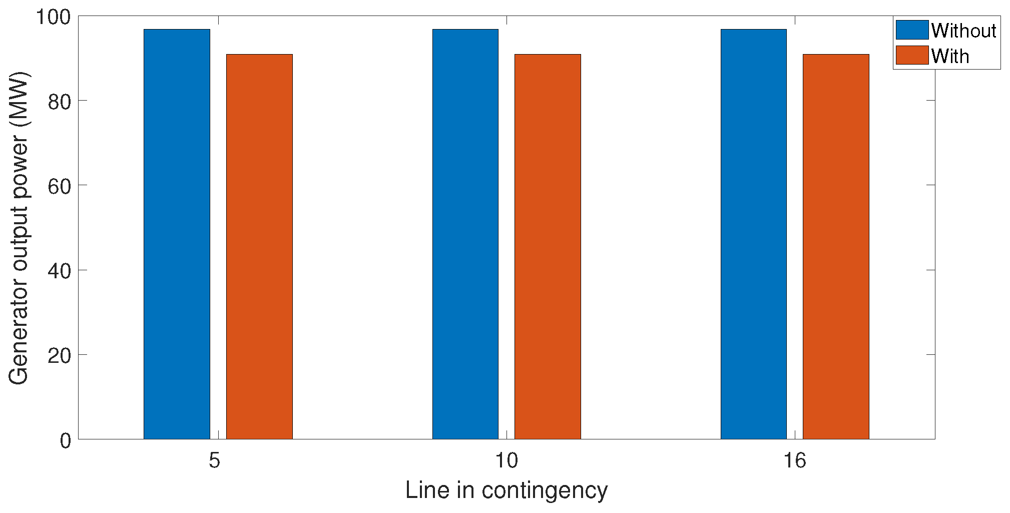
Figure 12.
Voltage and power dispatched in the extended power system prior to and after contingency of branch 5 (generation nodes are, respectively, nodes 1, 2, 3, 6, and 8).
Figure 12.
Voltage and power dispatched in the extended power system prior to and after contingency of branch 5 (generation nodes are, respectively, nodes 1, 2, 3, 6, and 8).

Figure 13.
Voltage and power dispatched in the extended power system prior to and after contingency of branch 10 (generation nodes are, respectively, nodes 1, 2, 3, 6, and 8).
Figure 13.
Voltage and power dispatched in the extended power system prior to and after contingency of branch 10 (generation nodes are, respectively, nodes 1, 2, 3, 6, and 8).
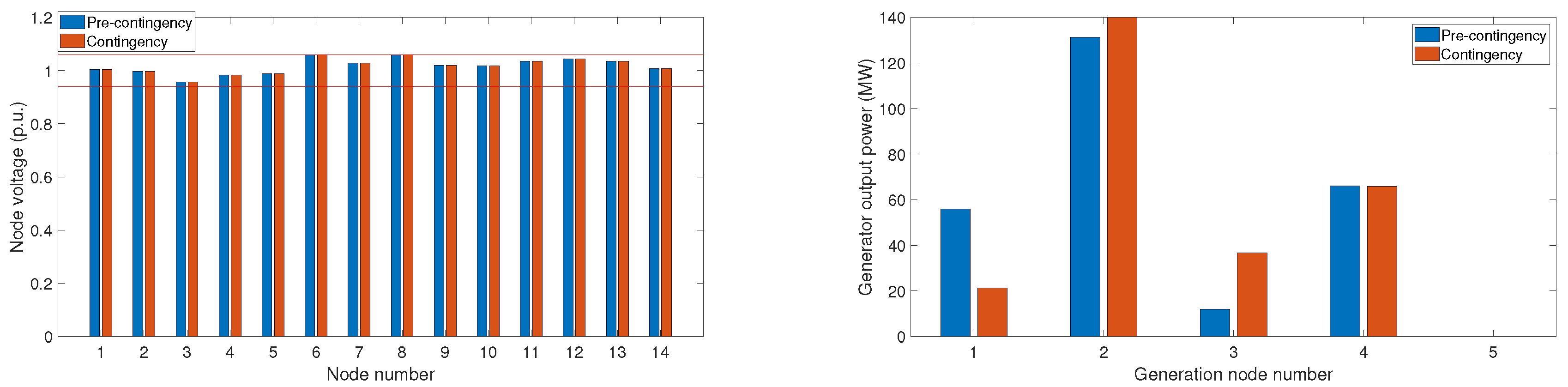
Figure 14.
Voltage and power dispatched in the extended power system prior to and after contingency of branch 16 (generation nodes are, respectively, nodes 1, 2, 3, 6, and 8).
Figure 14.
Voltage and power dispatched in the extended power system prior to and after contingency of branch 16 (generation nodes are, respectively, nodes 1, 2, 3, 6, and 8).

Figure 15.
Voltage and power dispatched in the extended power system with PV generation prior to and after contingency of branch 5 (generation nodes are, respectively, nodes 1, 2, 3, 6, and 8).
Figure 15.
Voltage and power dispatched in the extended power system with PV generation prior to and after contingency of branch 5 (generation nodes are, respectively, nodes 1, 2, 3, 6, and 8).
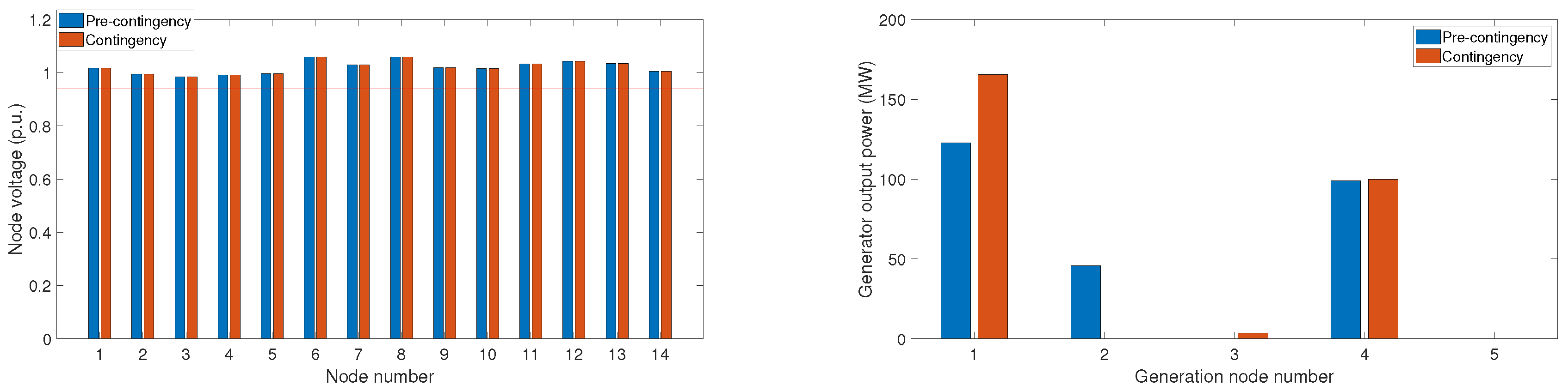
Figure 16.
Voltage and power dispatched in the extended power system with PV generation prior to and after contingency of branch 10 (generation nodes are, respectively, nodes 1, 2, 3, 6, and 8).
Figure 16.
Voltage and power dispatched in the extended power system with PV generation prior to and after contingency of branch 10 (generation nodes are, respectively, nodes 1, 2, 3, 6, and 8).

Figure 17.
Voltage and power dispatched in the extended power system with PV generation prior to and after contingency of branch 16 (generation nodes are, respectively, nodes 1, 2, 3, 6, and 8).
Figure 17.
Voltage and power dispatched in the extended power system with PV generation prior to and after contingency of branch 16 (generation nodes are, respectively, nodes 1, 2, 3, 6, and 8).

Figure 18.
Power dispatch of renewable generator number 4 without and with loadability restrictions for contingencies in branches 10 and 16.
Figure 18.
Power dispatch of renewable generator number 4 without and with loadability restrictions for contingencies in branches 10 and 16.

Figure 19.
Operational cost for each contingency and each strategy proposed, prior to and after the contingency takes place. (a) On the left: only thermal generation, (b) on the right: thermal generation and PV generation.
Figure 19.
Operational cost for each contingency and each strategy proposed, prior to and after the contingency takes place. (a) On the left: only thermal generation, (b) on the right: thermal generation and PV generation.

Table 1.
Variables that form an OPF problem using QCQP.
| Variable | Meaning |
|---|---|
| nVAR | Number of state variables (node voltages) |
| nEQ | Number of equality constraints |
| nINEQ | Number of inequality constraints |
| C, c | Objective function coefficient matrix, constant terms vector |
| A, a | Equality constraints coefficient matrix, constant terms vector |
| B, b | Inequality constraints coefficient matrix, constant terms vector |
Table 2.
Execution times obtained after implementation of QCQP and extended OPF strategies.
| QCQP | Extended OPF | |||
|---|---|---|---|---|
| Execution Time (s) | Execution Time (s) | |||
| Contingency Located at | Thermal Generation Only | Thermal Generation + PV Generation and Battery Storage | Thermal Generation Only | Thermal Generation + PV Generation and Battery Storage |
| Branch 5 | 0.531975 | 1.253313 | 0.412515 | 0.507896 |
| Branch 10 | 0.501589 | 0.939263 | 0.435760 | 0.517546 |
| Branch 16 | 0.588455 | 0.938105 | 0.439151 | 0.469477 |
© 2020 by the authors. Licensee MDPI, Basel, Switzerland. This article is an open access article distributed under the terms and conditions of the Creative Commons Attribution (CC BY) license (http://creativecommons.org/licenses/by/4.0/).
Share and Cite
MDPI and ACS Style
Leon, L.M.; Bretas, A.S.; Rivera, S. Quadratically Constrained Quadratic Programming Formulation of Contingency Constrained Optimal Power Flow with Photovoltaic Generation. Energies 2020, 13, 3310. https://doi.org/10.3390/en13133310
AMA Style
Leon LM, Bretas AS, Rivera S. Quadratically Constrained Quadratic Programming Formulation of Contingency Constrained Optimal Power Flow with Photovoltaic Generation. Energies. 2020; 13(13):3310. https://doi.org/10.3390/en13133310
Chicago/Turabian StyleLeon, Luis M., Arturo S. Bretas, and Sergio Rivera. 2020. "Quadratically Constrained Quadratic Programming Formulation of Contingency Constrained Optimal Power Flow with Photovoltaic Generation" Energies 13, no. 13: 3310. https://doi.org/10.3390/en13133310
Note that from the first issue of 2016, this journal uses article numbers instead of page numbers. See further details here.