Pseudo-Steady-State Parameters for a Well Penetrated by a Fracture with an Azimuth Angle in an Anisotropic Reservoir
by
 , ,
, ,
Guoqiang Xing
1,2 ,
,
Mingxian Wang
1,*,
Shuhong Wu
1,2,
Hua Li
1,2,
Jiangyan Dong
1,2 and
Wenqi Zhao
1 1
Research Institute of Petroleum Exploration and Development, China National Petroleum Corporation, Beijing 100083, China
2
State Key Laboratory of Enhanced Oil Recovery, Ministry of Science and Technology, Beijing 100083, China
*
Author to whom correspondence should be addressed.
Energies 2019, 12(12), 2449; https://doi.org/10.3390/en12122449
Submission received: 7 May 2019
/
Revised: 15 June 2019
/
Accepted: 21 June 2019
/
Published: 25 June 2019
(This article belongs to the Section H: Geo-Energy)
Abstract
:Many oil wells in closed reservoirs continue to produce in the pseudo-steady-state flow regime for a long time. The principal objective of this work is to investigate the characteristics of two key pseudo-steady-state parameters—pseudo-steady-state constant (bDpss) and pseudo-skin factor (S)—for a well penetrated by a fracture with an azimuth angle (θ) in an anisotropic reservoir. Firstly, a general analytical pressure solution for a finite-conductivity fracture with or without an azimuth angle in an anisotropic rectangular reservoir was developed by using the point-source function and spatial integral method, and two typical cases were employed to verify this solution. Secondly, with the asymptotic analysis method, the expressions of pseudo-steady-state constant and pseudo-skin factor were obtained on the basis of their definitions, and the effects of permeability anisotropy, fracture azimuth angle, fracture conductivity and reservoir shape on them were discussed in detail. Results show that all the bDpss-θ and S-θ curves are symmetric around the vertical line, θ = 90° and form a hump or groove shape. The optimized fracture direction in an anisotropic reservoir is perpendicular to the principal permeability axis. Furthermore, a new formula to calculate pseudo-skin factor was successfully proposed based on these two parameters’ relationship. Finally, as an application of pseudo-steady-state constant, a set of Blasingame format rate decline curves for the proposed model were established.
1. Introduction
Considering that steady state condition rarely occurs in reservoirs, pseudo-steady-state (PSS) flow regime is one of the most important regimes for all closed reservoirs [1,2]. This regime may last for a long time, and many oil or gas wells continue to produce in this regime; thus, a considerable productivity may be recovered from these reservoirs. Therefore, it is of great significance for a closed reservoir to investigate its characteristics in the PSS flow regime.
Pseudo-steady-state constant and pseudo-skin factor are two key parameters to reflect upon the property of PSS flow regime. The former parameter is an auxiliary variable to build up new rate decline curves, like “Fetkovich” format and “Blasingame” format, which can improve the precision of well test and is also an important method to estimate the hydrocarbon reserves in place and assess the recoverable amount of the oil from the reservoirs [3,4,5,6]. Moreover, Hagoort (2009) found that pseudo-steady-state constant can be used for the measurement of the productivity of the well in the PSS flow period [7]. He also obtained a useful relationship that pseudo-steady-state constant is the reciprocal of the dimensionless production index. The latter parameter is extremely useful to determine the productivity increase or decrease caused by partial penetration or slant of a well, or fracture configuration [8,9,10,11,12]. Cinco-Ley (1975) first introduced the definition of the pseudo-skin factor for a slanted well and demonstrated that the calculation of the pseudo-skin factor permitted evaluation of the well condition [8]. Ozkan (1988) used the pseudo-skin factor to compare the performance of horizontal wells to that of vertically fractured wells and unstimulated vertical wells [10]. Hydraulic fracturing can increase the productivity of tight porous medium. There are many solutions, including the analytical type, semi-analytical type, and numerical type, to investigate the flow efficiency of fractured wells in the transient period [13,14,15,16,17,18,19]. However, there are few researches focusing on the pseudo-steady-state problem of fractured wells. Based on the pseudo-skin factor for a uniform-flux inclined fracture presented by Cinco-ley [8], Jia et al. (2016) discussed the effect of inclination angle, fracture conductivity and permeability anisotropy on the pseudo-skin factor for a finite-conductivity inclined fracture connected to a slanted wellbore [12]. Their conclusions provide a theoretical basis for optimizing the well pattern and designing the reservoir stimulation.
Although the studies of PSS flow have been very common, the related studies of fractured wells in the anisotropic reservoirs are still rarely reported at present. Coordinate transformations, including rotation transformation and scaling transformation, are the main methods to deal with the issue of reservoir anisotropy. The principle of these methods is to convert the anisotropic system into the equivalent isotropic system [8,12,20,21,22,23,24,25]. Kucuk and Brigham (1979) transformed the Cartesian coordinates into the elliptical coordinates and solved the elliptical flow problems that existed in the infinite conductivity vertically fractured wells in anisotropic reservoirs [20]. Spivey and Lee (1999) established an equivalent isotropic system for a horizontal or hydraulically fractured well at an arbitrary azimuth in an anisotropic formation [24]. Cinco-Ley (1975) and Jia et al. (2015) presented a set of coordinate transformation system to investigate the transient pressure for an inclined fracture [8,12]. Using the scaling transformation, Xu et al. (2017) obtained an analytical solution for a finite-conductivity fracture at an arbitrary azimuth in a rectangular anisotropic reservoir [25]. On the basis of their work, PSS flow of these models can be easily discussed. However, coordinate rotation transformation is not appropriate for a rectangular reservoir, and coordinate scaling transformation may cause the fracture shape to change and cannot reflect the actual flow behavior in an anisotropic rectangular reservoir.
As introduced from the previous literature, in terms of the studies of fractured wells, except Spivey and Lee (1999) and Xu et al. (2017) [24,25], there is little research considering the effect of the fracture azimuth angle in an anisotropic reservoir. Due to the defects existed in the proposed approaches, the primary purpose of this work is to find a new way to deal with permeability anisotropy for a finite-conductivity fracture with an azimuth angle in an anisotropic rectangular reservoir and further to investigate its corresponding pseudo-steady-state parameters.
In this work, firstly, an analytical solution was obtained for a well penetrated by a vertical fracture with or without an azimuth angle in an anisotropic rectangular reservoir, and two cases were employed to validate this analytical solution. Secondly, the expressions of pseudo-steady-state constant and pseudo-skin factor for this model were derived in detail, and the influence of permeability anisotropy, fracture azimuth angle, fracture conductivity and reservoir shape on these two parameters were discussed. In addition, a new formula to calculate the pseudo-skin factor was obtained, and also a set of new Blasingame type curves for this model were established by using the pseudo-steady-state constant.
2. Physical Model
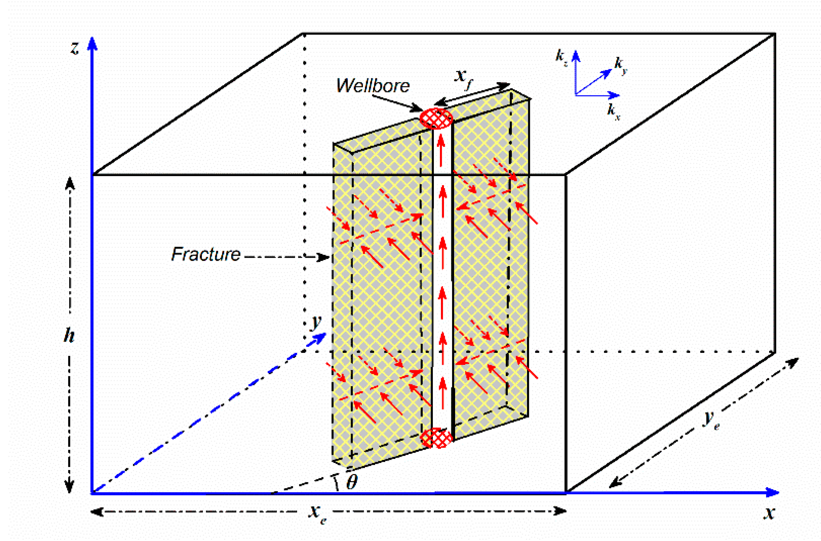
Figure 1 is a schematic illustration of a well penetrated by a vertical fracture with an azimuth angle in the anisotropic rectangular reservoir. In order to simplify the mathematical model, several basic assumptions are made as follows:
- (1)
- This rectangular reservoir is closed at every boundary, and it is anisotropic in the horizontal direction and its porous medium is homogeneous. It has a uniform thickness with constant porosity and its permeability in x and y direction are and , respectively.
- (2)
- Flow in this reservoir is considered to be a slightly compressible single-phase fluid with constant viscosity and total compressibility , and obeys Darcy’s law.
- (3)
- The reservoir is fully penetrated by a finite-conductivity vertical fracture, which lies at an arbitrary azimuth angle in the x-y plane ().
- (4)
- No fluid is assumed to flow at the fracture tip. The total flow contribution of the fracture to the wellbore is .
- (5)
- The half length of the fracture is assumed to have constant length , constant width and constant permeability .
- (6)
- Gravity effects are neglected and basic laminar flow occurs in the system.
3. Mathematical Model
To obtain the pseudo-steady-state parameters, we first developed a pseudo-steady-state solution of a fracture with an azimuth angle in an anisotropic rectangular reservoir. Figure 2 presents a detailed derivation process of the pseudo-steady-state solution, and the key of this process lies in the development of the model’s unsteady-state and pseudo-steady-state solution. The related derivation of STEP 1, STEP 2, STEP 3 and STEP 4 is presented in this section, and the detailed derivation of STEP 5 is given in Appendix A.
Gringarten and Ramey (1973) provided the basic instantaneous source function in an infinite slab reservoir under the closed boundary condition [26]:
where , .
The instantaneous point-source function in an anisotropic rectangular reservoir can be obtained by considering the intersection of a plane source in the x direction and a plane source in the y direction in a closed linear reservoir, where we do not consider the z-component.
By means of the superposition theorem [26], we obtained the pressure distribution in the anisotropic rectangular reservoir:
For the sake of the simplicity, a series of dimensionless variables are listed in Table 1.
Using these variables, we can obtain the dimensionless form for Equation (3):
where
Note that we do not take a coordinate scaling transformation to convert the anisotropic system into the equivalent isotropic system and all the derivations are conducted in the anisotropic system, which is different from the method of Xu et al. (2017) [25] and avoids the fracture deformation caused by the coordinate scaling transformation.
Applying the Laplace transform to Equation (4), we have the point-source solution for a rectangular reservoir in Laplace domain:
where . When , Equation (5) can be regressed to the solution of a vertical well in an isotropic rectangular reservoir.
According to the coordinate system in Figure 1, the following equations can be easily obtained ( is the fracture azimuth angle):
where and are the dimensionless coordinate along the fracture.
After substituting the above equations into the point-source solution (Equation (5)), taking as the integral variable and conducting the integral from −1 to 1, we can get the infinite-conductivity fracture pressure distribution under constant production rate:
Let
This pressure solution, Equation (6), can be sorted as follows:
Selecting the equivalent average pressure point presented by Gringarten et al. (1974): , , we can further obtain an approximate infinite-conductivity fracture solution in Laplace domain [27].
Because of the symmetry, it is not necessary to study all the values of azimuth angle. In this work, we only consider the azimuth angle’s range: . When , by using the traditional integral method, , and in Equation (7) can be simplified as:
Let the last term in the right side of Equation (10) equal to :
Equation (11) is not conducive to the rapid convergence. According to the following formula [28]:
Equation (11) can be converted to the following form, which is convenient to get a simple rapid algorithm:
where .
Substituting Equation (13) into Equations (8) and (10), the infinite-conductivity fracture equivalent pressure solution in an isotropic rectangular reservoir can be further expressed as follows:
where
When , the fracture is parallel to x axis and the above process related to the two terms, and , is not applicable to this case. However, we can directly substitute the equivalent average pressure point and into Equation (7), and easily obtain the corresponding equivalent pressure solution of the infinite-conductivity fracture at :
where
Therefore, using Equations (14) and (15), we can calculate the equivalent wellbore pressure of an infinite-conductivity fracture with or without an azimuth angle.
Wang et al. (2014) developed a conductivity influence function to deal with the flow in a finite-conductivity fracture [29]. Based on the result of Wang et al. (2014), for a well penetrated by a single finite-conductivity fracture with or without an azimuth angle, its pressure solution under constant rate can be written as follows:
where is the fracture conductivity influence function.
According to the Stehfest (1970) numerical inversion [30], the pressure solution in the real time domain can be written:
4. Model Validation
4.1. Validation of a Fractured Well in an Isotropic Rectangular Reservoir
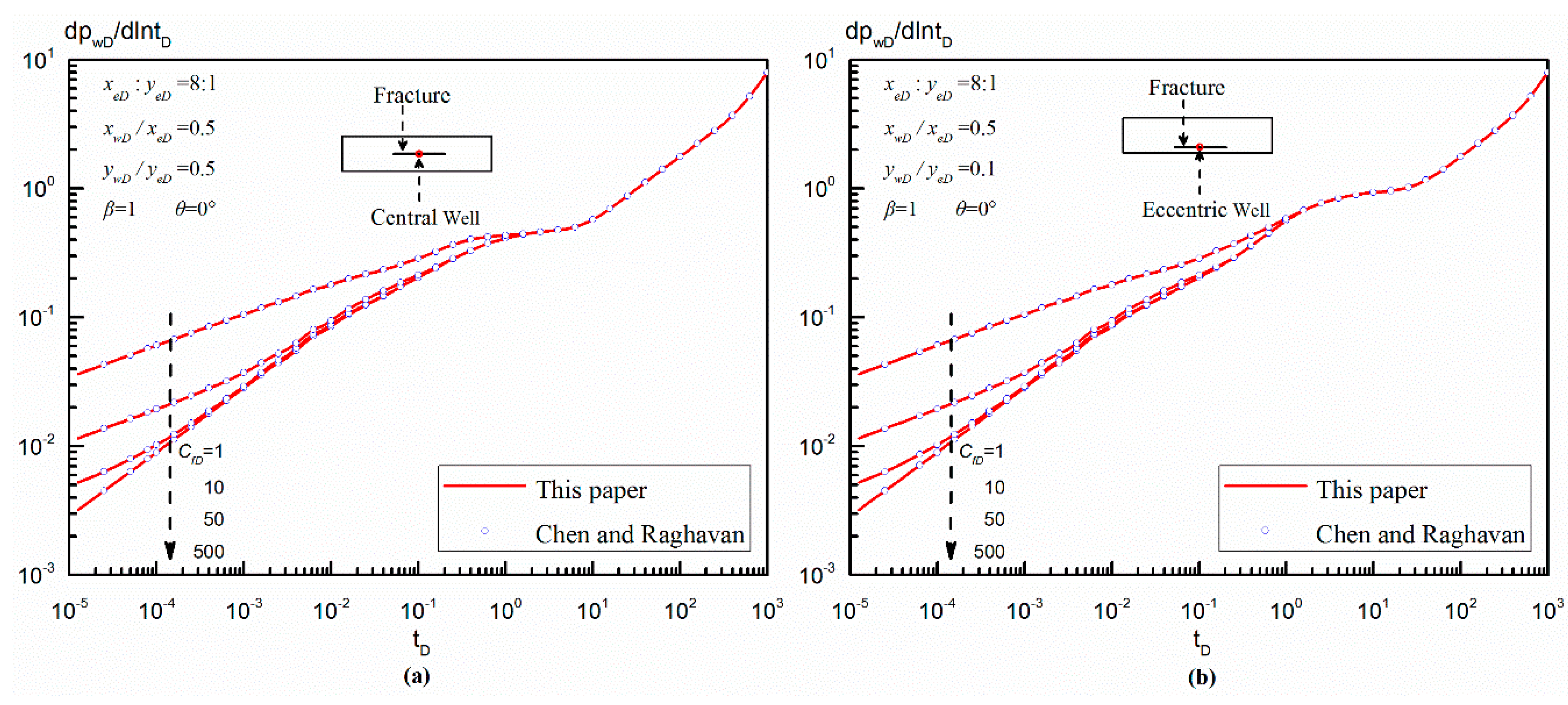
Chen and Raghavan (1997) presented a finite-conductivity fracture solution for a vertical fracture parallel to the x axis in an isotropic rectangular reservoir [31]. They considered two cases in an 8:1 rectangle reservoir: a well located at the center of the rectangle (, , , ), and a well located close to the rectangle’s longer side (, , , ). Obviously, these two scenarios are special cases of our model. Thus, we can validate our model by substituting the parameter values above into our model and comparing our results with Chen and Raghavan’s. Figure 3a,b show the comparison results of the dimensionless pressure at different fracture conductivity for a well located at the center of the rectangle and close to the rectangle’s longer side, respectively. It demonstrates that our results show excellent agreement with the work of Chen and Raghavan within the whole production life.
4.2. Validation of a Finite-Conductivity Fracture with an Azimuth Angle in an Anisotropic Reservoir
As mentioned above, Xu et al. (2017) presented a solution for a finite-conductivity fracture with an azimuth angle in an anisotropic rectangular reservoir by using the scaling transformation [25]. Figure 4 shows the comparison of the dimensionless pressure derivative for a vertical fracture at different azimuth angle. As presented in Figure 4, the pressure derivative of our model is in good agreement with that of Xu et al. The deviations of the results are mainly at early time, which may be caused by the different approaches to deal with the reservoir anisotropy.
5. Pseudo-Steady-State Flow Parameters
Pseudo-steady-state constant and pseudo-skin factor are two key parameters in the PSS flow period, which can help us to understand this period’s characteristics and also analyze this period’s productivity. In this section, pseudo-steady-state constant and pseudo-skin factor corresponding to our model were obtained with the asymptotic analysis method.
5.1. Pseudo-Steady-State Constant
Pratikno et al. (2003) proposed a pseudo-steady-state formula when developing an analytical solution for a single finite-conductivity fracture in the isotropic circular reservoir [6]:
For an isotropic circular reservoir, pseudo-steady-state constant, bDpss, is only related to the dimensionless reservoir drainage radius and fracture conductivity, CfD. Pseudo-steady-state constant is of great importance for the analysis of new rate decline curves. The general definitions of the variables used for “Fetkovich” format rate decline curves can be written as follows [3]:
In order to eliminate the possibility of the multiple solutions and errors existed in well test, Blasingame et al. (1989) presented the integral average method [32]. The auxiliary “decline” variables used for “Blasingame” format rate decline curves are given by:
- (1)
- Rate integral function:
- (2)
- Rate integral-derivative function:
Based on the pressure solution under constant rate (Equation (16)), combining the Duhamel principle and the above equations, we can set up new Blasingame type curves for a well penetrated by a finite-conductivity vertical fracture in an anisotropic rectangular reservoir. The key to establish these type curves is to derive the pseudo-steady-state constant with the asymptotic analysis method.
Through a series of asymptotic analysis, we obtain an approximate pressure solution for our model in the PSS flow regime (Appendix A). Its pseudo-steady-state constant is further obtained:
At ,
At ,
The derivation of this parameter is presented in detail in Appendix A. We can note that for a well penetrated by a vertical fracture with or without an azimuth angle in an anisotropic rectangular reservoir, or , is independent of time, but this parameter is closely related to permeability anisotropy, fracture conductivity, fracture azimuth angle, well location, and rectangular boundary condition.
5.2. Pseudo-Skin Factor
For an anisotropic rectangular reservoir, in the PSS flow regime, there is a difference between the wellbore pressure for a well penetrated by a vertical fracture with an azimuth angle, , and the wellbore pressure for a well penetrated by a vertical fracture parallel to the x axis, . This difference remains constant and can be handled as a pseudo-skin factor [8,12,33], which can be defined as:
Fracture azimuth angle, , in the first term of the right-hand side of Equation (26), can take any value. Obviously, like the pseudo-steady-state constant, the pseudo-skin factor for our model is also dependent on permeability anisotropy, fracture conductivity, fracture azimuth angle, and rectangular boundary condition.
6. Results and Discussion
In this section, we mainly focus on the effects of permeability anisotropy, fracture conductivity, reservoir shape, and fracture azimuth angle on PSS flow. The relationship between pseudo-steady-state constant and pseudo-skin factor was also discussed. Finally, as an application, we established a set of Blasingame format curves for this model by using the derived pseudo-steady-state constant.
6.1. Analysis of Parameters’ Influence on Pseudo-Steady-State Flow
6.1.1. Permeability Anisotropy
According to the definition of permeability anisotropy, the reservoir tends to be isotropic when approaches to one, and when the seepage capacity in the x-axis direction becomes stronger as the value of permeability anisotropy increases, and when the seepage capacity in the y-axis direction becomes stronger as the value of permeability anisotropy decreases.
Figure 5a,b demonstrate the effects of permeability anisotropy, and on the pseudo-steady-state constant at different fracture azimuth angles, respectively. As is displayed in Figure 5a, when , for the same value of permeability anisotropy, the pseudo-steady-state constant first goes up and then goes down as the fracture azimuth angle increases from 0° to 180°. The curves are symmetric around the vertical line, and form a hump shape. With the increase of permeability anisotropy, the pseudo-steady-state constant decreases and the corresponding hump gradually flattens out until it becomes a horizontal line for the same other parameters’ value. Similarly, it is shown in Figure 5b that when , the curves are also symmetric around the vertical line, . But, the pseudo-steady-state constant first goes down and then goes up as the fracture azimuth angle increases from 0° to 180° and forms a groove shape, which is different from the curves’ shape in Figure 5a. With the increase of permeability anisotropy, the pseudo-steady-state constant decreases and the corresponding groove gradually deepens for the same other parameters’ value.
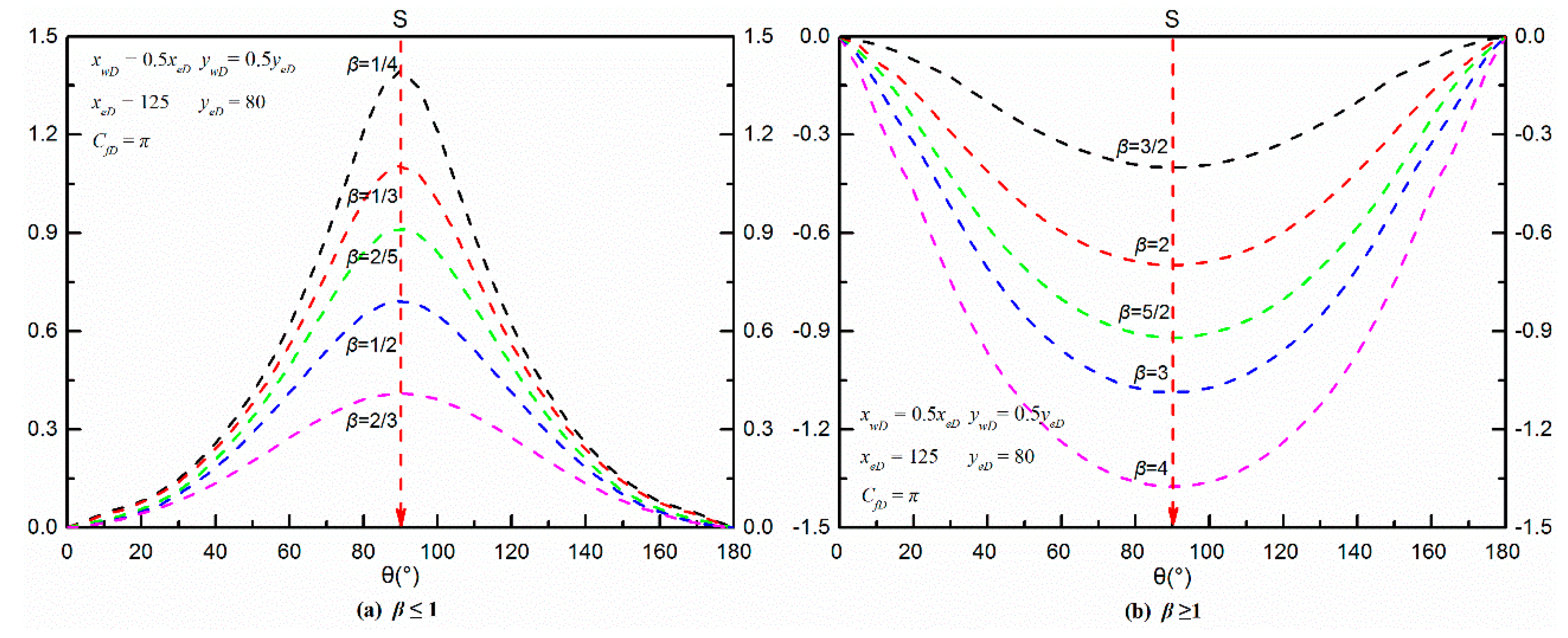
Figure 6a,b show the influence of permeability anisotropy, and , on the pseudo-skin factor at different fracture azimuth angle, respectively. Compared with Figure 6a,b, the shape and trend of the curves are similar to those of the curves for the same parameters’ value, but the shape of the hump and groove in the curves is more striking than that in the curves, which seems that there is a stretching transformation.
Pseudo-skin factor can directly reflect the stimulation effect in the PSS flow regime, but pseudo-steady-state constant cannot. According to the definition of pseudo-skin factor, a negative pseudo-skin factor indicates an increase in well productivity compared with the fracture parallel to x axis, and a positive pseudo-skin factor represents the stimulation effect of the fracture with an azimuth angle is not better than that of the fracture parallel to x axis. Therefore, from the curves in Figure 6, we can find out an optimal fracture azimuth angle for an anisotropic reservoir. When , all the calculated pseudo-skin factors are positive, which indicates the optimized fracture direction is perpendicular to the principal permeability axis (y axis) or parallel to the secondary permeability axis (x axis). However, when , all the calculated pseudo-skin factors are negative, which also demonstrates that the optimized fracture direction is perpendicular to the principal permeability axis, but the corresponding principal permeability axis is x axis. These results provide a theoretical basis for optimizing the stimulation in an anisotropic reservoir.
6.1.2. Fracture Conductivity
Figure 7 and Figure 8 present the effects of fracture conductivity () on pseudo-steady-state constant and pseudo-skin factor at varied fracture azimuth angles, respectively. The shape and trend of the and curves for different fracture conductivity are similar to the previous case of different permeability anisotropy, (Figure 5b and Figure 6b). As presented in Figure 7, the pseudo-steady-state constant and pseudo-skin factor first go down and then up as the fracture azimuth angle increases from 0° to 180° and also form a groove shape. As the fracture conductivity increases, the pseudo-steady-state constant gradually increases, but increases more and more slowly, even when the fracture conductivity is larger than 100π, the change of pseudo-steady-state constant can be neglected. Interestingly, all the curves for different fracture conductivity are perfectly coincident (Figure 8) and it demonstrates that fracture conductivity has no obvious effect on the pseudo-skin factor. In fact, it can be interpreted that the pseudo-steady-state flow is controlled by reservoir boundary condition and has nothing to do with the fracture conductivity, which only affects the early flow regime. For the optimization of fracture conductivity, we need to study its early unsteady flow behavior.
6.1.3. Reservoir Shape
As mentioned earlier, PSS flow is mainly controlled by reservoir boundary, thus reservoir shape needs to be investigated in detail. Here, we keep the total drainage area of this rectangular reservoir constant and study the effects of reservoir shape on PSS flow by varying the length of the rectangular reservoir. In this work, we set the total area () as 10,000 and take the length of the rectangle, , equal to 50, 75, 100, 125 and 150, respectively.
Figure 9 exhibits the effects of reservoir shape on the pseudo-steady-state constant at different azimuth angle and permeability anisotropy. For a given permeability anisotropy, the shape and trend of the curves are also similar to the previous case of different permeability anisotropy (Figure 5a,b). The pseudo-steady-state constant increases gradually with the increase of the length for the other parameters’ value.
Corresponding to the parameter value in Figure 9, Figure 10 demonstrates the effects of reservoir shape on the pseudo-skin factor at varied azimuth angle and permeability anisotropy. We can easily find that the optimized fracture direction for a given permeability anisotropy is consistent with the previous results. However, the curves for different reservoir shape at the same permeability anisotropy almost overlap together, which indicates that the optimized fracture direction almost has nothing to do with the reservoir shape. Therefore, in an anisotropic rectangular reservoir, the optimized fracture direction mainly depends on permeability anisotropy.
6.2. Analysis of the Relationship between Pseudo-Steady-State Constant and Pseudo-Skin Factor
When investigating the effects of different parameters on pseudo-steady-state constant and pseudo-skin factor, we can note that the trend of the and curves is similar for the same parameters’ values, which tempts us to discuss whether there is an intrinsic relationship between these two parameters.
In Appendix A, we formulated the approximate equivalent pressure for a well penetrated by a finite-conductivity fracture in the PSS flow regime. For the fracture with an azimuth angle, its approximate equivalent pressure in the PSS flow regime can be sorted as Equation (26).
And for the fracture parallel to x axis (), its approximate equivalent pressure in the PSS flow regime can be sorted as:
In the PSS flow regime, we can have the following approximations:
Based on the definition of the pseudo-skin factor, the relationship between the pseudo-skin factor and the pseudo-steady-state constant can be derived as follows:
where is the pseudo-steady-state constant for a fully penetrating fracture with an azimuth angle in an anisotropic rectangular reservoir, and is the pseudo-steady-state constant for a fully penetrating fracture parallel to x axis () in an anisotropic rectangular drainage area.
Based on Equation (30), we can first calculate the pseudo-steady-state constant, and , and then use this relationship to calculate the pseudo-skin factor. Therefore, Equation (30) can be regarded as a new formula to compute the pseudo-skin factor.
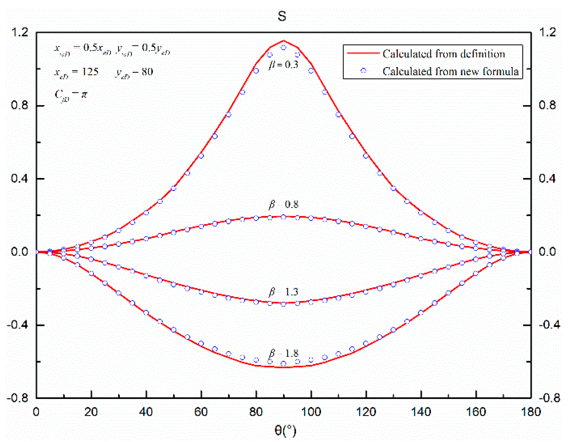
Figure 11 shows the comparison results of the pseudo-skin factor calculated from its definition and this new formula. The well agreement between the calculation results of these two methods at different azimuth angles can be seen in this figure. When the azimuth angle is close to 90°, there is a slight discrepancy between the pseudo-skin factors calculated from these two methods, which may be caused by calculating the trigonometric functions in the expressions. This comparison indicates that this new formula presented in this study is reliable.
6.3. Establishment of Blasingame Format Rate Decline Curves by Using Pseud-Steady-State Constant
Pseudo-skin factor can be used to compare the stimulation effect and optimize the fracture direction, but pseudo-steady-state constant has no physical meaning. However, as an important auxiliary variable, pseudo-steady-state constant can help us to establish “Fetkovich” or “Blasingame” format rate decline curves, then we can further extend our study from pseudo-steady-state flow to unsteady flow [6]. These new format rate decline curves can deal with the problem of both variable flow rate and variable wellbore pressure [5], thus our mathematical model is not subject to wellbore condition any more. Meanwhile, based on these curves, we could recognize the model’s flow regimes, analyze its flow behavior and also conduct the well test [34,35,36]. Hence, all the above study depends on the pseudo-steady-state constant. Here, as an application of pseudo-steady-state constant, we established a set of Blasingame format rate decline curves for the proposed model in this study.
Figure 12 shows the whole flow process of a well penetrated by a finite-conductivity fracture with the azimuth angle of 45°, including the unsteady flow in the early time and the pseudo-steady-state flow in the late time. As is described in Figure 12, the flow progress in this model can be divided into five flow regimes: bilinear flow regime, linear flow regime, radial flow regime, transition flow regime and pseudo-steady-state flow regime.
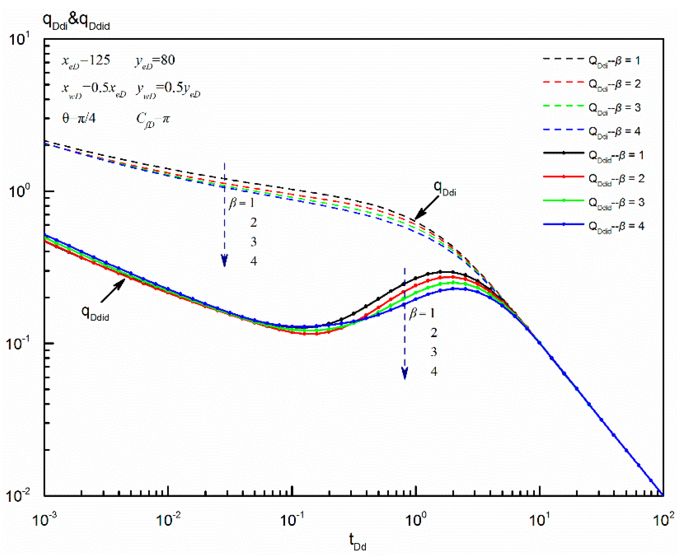
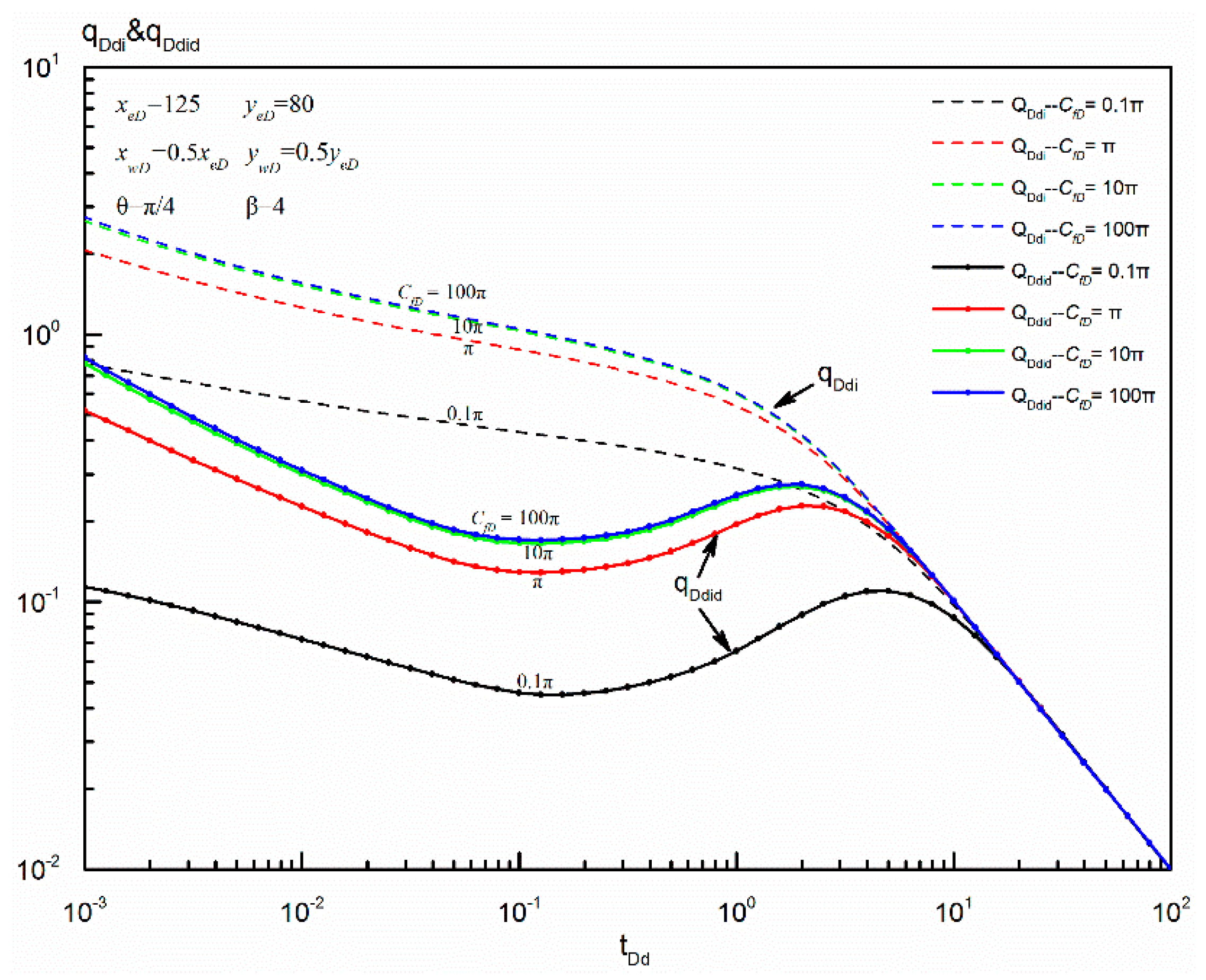
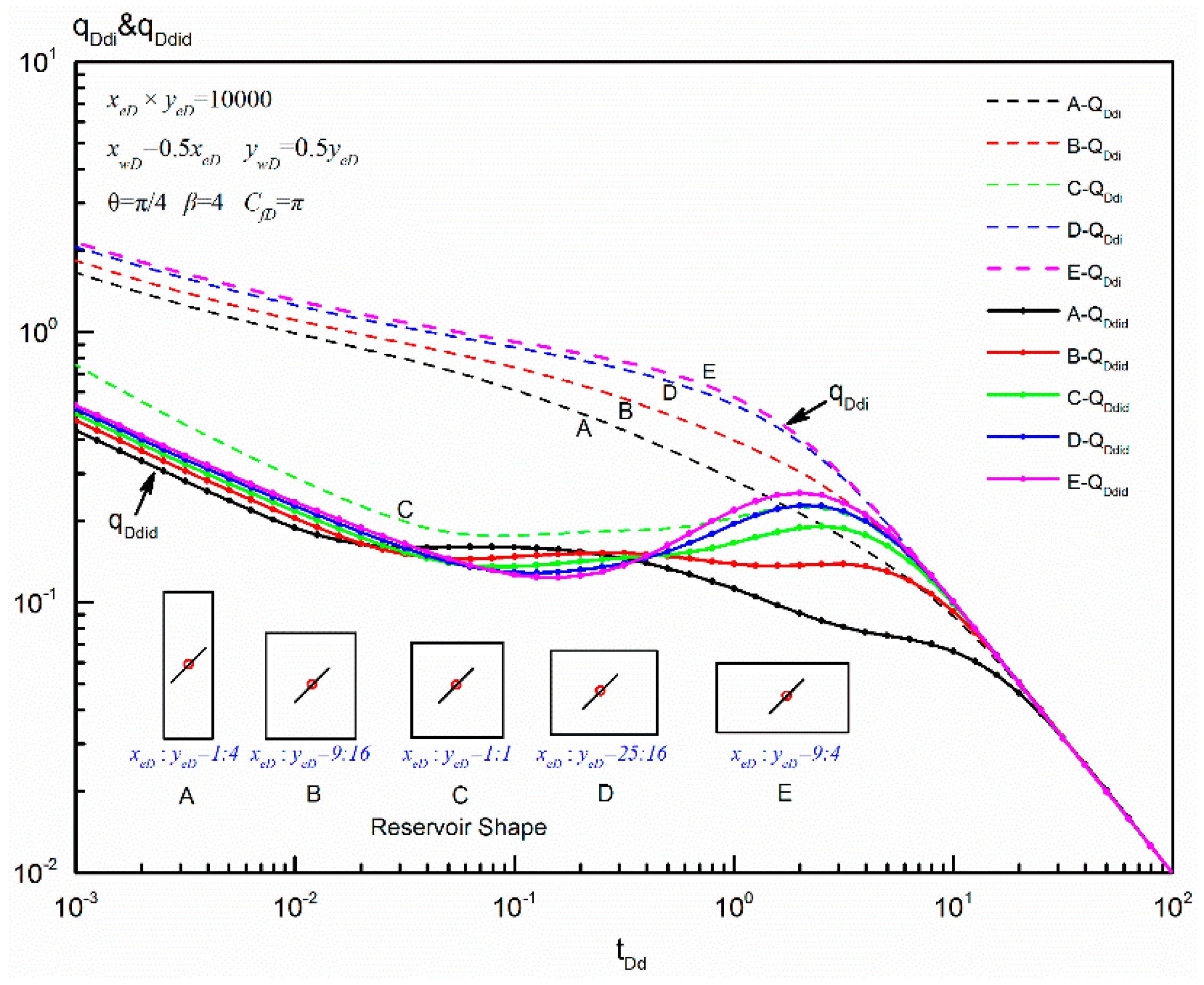
Figure 13, Figure 14, Figure 15 and Figure 16 present the Blasingame format curves for the previous parameters, including fracture azimuth angle, permeability anisotropy, fracture conductivity and reservoir shape, respectively. The curves (dash lines) and the curves (solid lines with symbol) have a similar decline trend, but the latter ones are more salient in terms of typical features. Fracture azimuth angle mainly affects early-time flow, and the effect of permeability anisotropy is concentrated in the intermediate-time flow. But, fracture conductivity has a strong effect on both the early- and intermediate-time flow and so does reservoir shape. We also can find that all the curves in each figure normalize in the pseudo-steady-state flow regime. Based on the flow regime identification and sensitivity analysis, we can estimate the formation property parameters via well test interpretation.
In addition, as shown in Figure 13, the value of in the early-time flow period increases gradually with the increase of fracture azimuth angle. Because of the symmetry in this research, we can obtain a peak value when the fracture azimuth angle is equal to 90°, which verifies the previous point that the optimized fracture direction is perpendicular to the principal permeability axis. Meanwhile, Figure 15 demonstrates that the value of in the early- and intermediate-time flow period increases as the fracture conductivity increases, but the value of will not increase any more when the fracture conductivity is larger than 10π (closed to 30). Therefore, the optimized fracture conductivity is about 30 for the reservoirs under the given parameters’ value in Figure 15 and it is not necessary to pursue a larger fracture conductivity in hydraulic fracturing.
7. Conclusions
This paper investigated two important pseudo-steady-state parameters for a well penetrated by a finite-conductivity fracture with an azimuth angle in an anisotropic rectangular reservoir. From the results of this investigation, the following conclusions can be drawn:
- (1)
- The equivalent wellbore pressure solution for a single finite-conductivity fracture with or without an azimuth angle in an anisotropic rectangular reservoir was developed by using the point-source function and spatial integral method. It showed excellent agreement with the work of Chen and Raghavan, and Xu et al., which demonstrates that the proposed pressure solution is reliable.
- (2)
- An approximate pressure solution for this model in the pseudo-steady-state flow regime was derived with the asymptotic analysis method. The expressions of pseudo-steady-state constant and pseudo-skin factor were further obtained on the basis of their definitions.
- (3)
- Except for the isotropic reservoirs, all the and curves are symmetric around the vertical line, and form a hump or groove shape. Fracture conductivity and reservoir shape almost have no effect on the pseudo-skin factor for a given anisotropic reservoir. The optimized fracture direction mainly depends on permeability anisotropy and is perpendicular to the principal permeability axis.
- (4)
- Based on the definitions of pseudo-steady-state constant and pseudo-skin factor, a new formula to calculate the pseudo-skin factor was successfully proposed with their relationship. The comparison of the pseudo-skin factors calculated from its definition and the new formula at different azimuth angle verified the reliability of this new formula.
- (5)
- As an application of pseudo-steady-state constant, a set of Blasingame format rate decline curves for the proposed model were established. Five flow regimes can be observed on the typical Blasingame format curves. Fracture azimuth angle mainly affects the early-time flow, and permeability anisotropy mainly affects the intermediate-time flow. But fracture conductivity and reservoir shape have a strong effect on both the early- and intermediate-time flow. All the curves normalize in the pseudo-steady-state flow regime. Additionally, there is an optimized fracture conductivity for a given anisotropic rectangular reservoir.
Author Contributions
All authors have contributed to this work. G.X. and M.W. contributed equally to this work and proposed the original idea for this paper. G.X. established the mathematical model and wrote the main manuscript text. As the corresponding author, M.W. made substantial contributions to the conception/design of the work. S.W., H.L., J.D. and W.Z. contributed to the modeling, programming, and results analysis and discussion.
Funding
This research was funded by the PetroChina Scientific Study and Technical Development Project (2017A-0906) and National Science and Technology Major Project of China (No. 2016ZX05046-003).
Acknowledgments
The authors acknowledge that this study was funded by the PetroChina Scientific Study and Technical Development Project (2017A-0906) and National Science and Technology Major Project of China (No. 2016ZX05046-003).
Conflicts of Interest
The authors declare that they have no competing interests.
Nomenclature
| Field Variables | |
| Distance in the x axis, m | |
| Distance in the y axis, m | |
| Distance in the x or y axis, m | |
| Reservoir length in the x axis, m | |
| Reservoir length in the y axis, m | |
| Reservoir length in the x or y axis, m | |
| Reservoir thickness, m | |
| Fracture half length, m | |
| Fracture width, m | |
| Permeability in the x-axis, 10−3μm2 | |
| Permeability in the y-axis, 10−3μm2 | |
| Equivalent system permeability, 10−3μm2 | |
| Fracture permeability, 10−3μm2 | |
| Angle between x axis and the extension direction of fracture, deg | |
| Reservoir initial pressure, MPa | |
| Porosity, fraction | |
| Fluid viscosity, mPa·s | |
| Total compressibility, 1/MPa | |
| Permeability anisotropic factor | |
| Wellbore flow rate, m3/d | |
| Principal diffusivities | |
| Correlation coefficient, n = 0,1,2…… | |
| Dimensionless Variables | |
| Dimensionless pressure in real time domain | |
| Dimensionless pressure in Laplace domain | |
| Dimensionless point-source solution in an anisotropic rectangular reservoir in Laplace domain | |
| Dimensionless pressure for an infinite-conductivity fracture in real time domain | |
| Dimensionless pressure for an infinite-conductivity fracture in Laplace domain | |
| Dimensionless pressure for an infinite-conductivity fracture paralleled to the x axis in real time domain | |
| Dimensionless pressure for an infinite-conductivity fracture paralleled to the x axis in Laplace domain | |
| Dimensionless pseudo-steady-state pressure in real time domain | |
| Dimensionless time | |
| Dimensionless time based on drainage area | |
| Dimensionless decline time | |
| Dimensionless pseudo-steady-state constant | |
| Dimensionless decline rate | |
| Dimensionless decline rate integral | |
| Dimensionless decline rate integral derivative | |
| Dimensionless distance in the x axis | |
| Dimensionless distance in the y axis | |
| Dimensionless reservoir length in the x axis | |
| Dimensionless reservoir width in the y axis | |
| Dimensionless wellbore location in the x axis | |
| Dimensionless wellbore location in the y axis | |
| Dimensionless coordinate in the x axis | |
| Dimensionless coordinate in the y axis | |
| Dimensionless fracture conductivity | |
| Impact function of dimensionless fracture conductivity in real time domain | |
| Impact function of dimensionless fracture conductivity in Laplace domain | |
| Dimensionless coefficient, i = 1, 2, 3…… | |
| Dimensionless coefficient related to and | |
| Dimensionless pseudo-skin factor | |
| Dimensionless time variable in Laplace domain | |
| Dimensionless integral variable | |
| Dimensionless coefficient, n = 0, 1, 2…… | |
| Dimensionless pseudo-steady-state coefficient, i = 1, 2 | |
| Dimensionless coefficient, i = 1, 2 | |
| Dimensionless productivity index | |
Appendix A. Derivation of Our Model’s Pseudo-Steady-State Constant
For a well penetrated by a finite-conductivity fracture in an anisotropic rectangular reservoir, the key to derive the pseudo-steady-state constant lies in obtaining an approximate pressure solution for this mode in the PSS flow regime.
The equivalent wellbore pressure solutions for the fracture with or without an azimuth angle are different. Thus, here we studied these two cases separately.
(1) When the azimuth angle ,
where
Gradshteyn and Ryzhik (2014) presented a series of useful expressions [28], which are easy for us to simplify the above equations:
Then, can be simplified as,
Considering that the dimensionless time in the PSS flow regime is close to infinite and correspondingly the Laplace variable, , tends to zero, can be further sorted as follows:
Similarly, when , , the sum of and can be simplified:
Thus, we can obtain an approximate pressure solution in the PSS flow regime:
Employing the inversion theorem of the Laplace transformation to Equation (A8), we can easily obtain the real space form of this approximate pressure solution.
In the PSS flow regime, based on the result of Riley et al. (1991) [37], Wang et al. (2012) presented an approximate formula for the conductivity influence function in the real space [38], which only depends on the fracture conductivity in this regime:
Therefore, this approximate pressure solution can be further expressed as:
Recalling the general identity for PSS flow [6], we have:
When , we finally got our model’s pseudo-steady-state constant:
(2) When the azimuth angle, ,
where
When , , and can be simplified as:
In the PSS flow regime, employing the inversion theorem of the Laplace transformation to Equations (A15) and (A16), and combining with Equation (A10), we can obtain the approximate pressure for the fracture parallel to the x axis:
Similarly, recalling the general identity for PSS flow [6], we have:
when , we can get the pseudo-steady-state constant for the fracture parallel to the x axis:
References
- Czarnota, R.; Stopa, J.; Janiga, D.; Kosowski, P.; Wojnarowski, P. Semianalytical horizontal well length optimization under pseudosteady-state conditions. In Proceedings of the IEEE 2nd International Conference on Smart Grid and Smart Cities (ICSGSC 2018), Kuala Lumpur, Malaysia, 12–14 August 2018; pp. 68–72. [Google Scholar]
- Ghahri, P.; Jamiolahmadi, M.; Alatefi, E.; Wilkinson, D.; Dehkordi, F.S.; Hamidi, H. A new and simple model for the prediction of horizontal well productivity in gas condensate reservoirs. Fuel 2018, 223, 431–450. [Google Scholar] [CrossRef] [Green Version]
- Fetkovich, M.J. Decline curve analysis using type curves. J. Pet. Technol. 1980, 32, 1065–1077. [Google Scholar] [CrossRef]
- McCray, T.L. Reservoir Analysis Using Production Decline Data and Adjusted Time. Ph.D. Thesis, A&M University, College Station, TX, USA, 1990. [Google Scholar]
- Blasingame, T.A.; McCray, T.L.; Lee, W.J. Decline Curve Analysis for Variable Pressure Drop/Variable Flowrate Systems. In Proceedings of the SPE Gas Technology Symposium, Houston, TX, USA, 22–24 January 1991. [Google Scholar]
- Pratikno, H.; Rushing, J.A.; Blasingame, T.A. Decline curve analysis using type curves-fractured wells. In Proceedings of the SPE Annual Technical Conference and Exhibition, Denver, CO, USA, 5–8 October 2003. [Google Scholar]
- Hagoort, J. The productivity of a well with a vertical infinite-conductivity fracture in a rectangular closed reservoir. SPE J. 2009, 14, 715–720. [Google Scholar] [CrossRef]
- Cinco-Ley, H.; Ramey, H.J., Jr.; Miller, F.G. Unsteady-state pressure distribution created by a well with an inclined fracture. In Proceedings of the Fall Meeting of the Society of Petroleum Engineers of AIME, Dallas, TX, USA, 28 September–1 October 1975. [Google Scholar]
- Reynolds, A.C.; Chen, J.C.; Raghavan, R. Pseudoskin factor caused by partial penetration. J. Pet. Technol. 1984, 36, 2197–2210. [Google Scholar] [CrossRef]
- Ozkan, E. Performance of horizontal wells. Ph.D. Thesis, Tulsa University, Tulsa, OH, USA, 1988. [Google Scholar]
- Tang, Y.; Ozkan, E.; Kelkar, M.; Yildiz, T. Fast and accurate correlations to compute the perforation pseudoskin and productivity of horizontal wells. In Proceedings of the SPE Annual Technical Conference and Exhibition, New Orleans, LA, USA, 30 September–3 October 2001. [Google Scholar]
- Jia, P.; Cheng, L.; Huang, S.; Liu, H. Pressure-transient analysis of a finite-conductivity inclined fracture connected to a slanted wellbore. SPE J. 2016, 21, 522–537. [Google Scholar] [CrossRef]
- Stopa, J.; Wiśniowski, R.; Wojnarowski, P.; Janiga, D.; Skrzypaszek, K. Integrated approach to drilling project in unconventional reservoir using reservoir simulation; E3S Web of Conferences. EDP Sci. 2018, 35, 01002. [Google Scholar]
- Jia, P.; Cheng, L.; Huang, S.; Xue, Y.; Clarkson, C.R.; Williams-Kovacs, J.D.; Wang, D. Dynamic coupling of analytical linear flow solution and numerical fracture model for simulating early-time flowback of fractured tight oil wells (planar fracture and complex fracture network). J. Pet. Sci. Eng. 2019, 177, 1–23. [Google Scholar] [CrossRef]
- Kong, B.; Chen, S. Numerical simulation of fluid flow and sensitivity analysis in rough-wall fractures. J. Pet. Sci. Eng. 2018, 168, 546–561. [Google Scholar] [CrossRef]
- Dejam, M. Advective-diffusive-reactive solute transport due to non-Newtonian fluid flows in a fracture surrounded by a tight porous medium. Int. J. Heat Mass Transf. 2019, 128, 1307–1321. [Google Scholar] [CrossRef]
- Wu, Z.W.; Cui, C.Z.; Lv, G.Z.; Bing, S.X.; Cao, G. A multi-linear transient pressure model for multistage fractured horizontal well in tight oil reservoirs with considering threshold pressure gradient and stress sensitivity. J. Pet. Sci. Eng. 2019, 172, 839–854. [Google Scholar] [CrossRef]
- Wu, S.H.; Xing, G.Q.; Cui, Y.D.; Wang, B.H.; Shi, M.Y.; Wang, M.X. A semi-analytical model for pressure transient analysis of hydraulic reorientation fracture in an anisotropic reservoir. J. Pet. Sci. Eng. 2019, 179, 228–243. [Google Scholar] [CrossRef]
- Luo, W.J.; Tang, C.F. Pressure-transient analysis of multiwing fractures connected to a vertical wellbore. SPE J. 2015, 20, 360–367. [Google Scholar] [CrossRef]
- Kucuk, F.; Brigham, W.E. Transient flow in elliptical systems. SPE J. 1979, 19, 401–410. [Google Scholar] [CrossRef]
- Kuchuk, F.J.; Goode, P.A.; Wilkinson, D.J.; Thambynayagam, R.K.M. Pressure-transient behavior of horizontal wells with and without gas cap or aquifer. SPE Form. Eval. 1991, 6, 86–94. [Google Scholar] [CrossRef]
- Ozkan, E.; Raghavan, R. New solutions for well-test-analysis problems: Part 1-analytical considerations. SPE Form. Eval. 1991, 6, 359–368. [Google Scholar] [CrossRef]
- Yildiz, T.; Ozkan, E. Influence of Areal Anisotropy on Horizontal Well Performance. In Proceedings of the SPE Annual Technical Conference and Exhibition, San Antonio, TX, USA, 5–8 October 1997. [Google Scholar]
- Spivey, J.P.; Lee, W.J. Estimating the pressure-transient response for a horizontal or a hydraulically fractured well at an arbitrary orientation in an anisotropic reservoir. SPE Reserv. Eval. Eng. 1999, 2, 462–469. [Google Scholar] [CrossRef]
- Xu, W.; Wang, X.; Xing, G.; Wang, J. Pressure-transient analysis for a vertically fractured well at an arbitrary azimuth in a rectangular anisotropic reservoir. J. Pet. Sci. Eng. 2017, 159, 279–294. [Google Scholar] [CrossRef]
- Gringarten, A.C.; Ramey, H.J., Jr. The use of source and Green’s functions in solving unsteady-flow problems in reservoirs. SPE J. 1973, 13, 285–296. [Google Scholar]
- Gringarten, A.C.; Ramey, H.J., Jr.; Raghavan, R. Unsteady-state pressure distributions created by a well with a single infinite-conductivity vertical fracture. SPE J. 1974, 14, 347–360. [Google Scholar] [CrossRef]
- Gradshteyn, I.S.; Ryzhik, I.M. Table of Integrals, Series, and Products; Academic Press: London, UK, 2007. [Google Scholar]
- Wang, X.; Luo, W.; Hou, X.; Wang, J. Pressure transient analysis of multi-stage fractured horizontal wells in boxed reservoirs. Petrol. Explor. Dev. 2014, 41, 82–87. [Google Scholar] [CrossRef]
- Stehfest, H. Algorithm 368: Numerical inversion of Laplace transforms. Commun. ACM 1970, 13, 47–49. [Google Scholar] [CrossRef]
- Chen, C.C.; Raghavan, R.A. Multiply-fractured horizontal well in a rectangular drainage region. SPE J. 1997, 2, 455–465. [Google Scholar] [CrossRef]
- Blasingame, T.A.; Johnston, J.L.; Lee, W.J. Type-curve analysis using the pressure integral method. In Proceedings of the SPE California Regional Meeting, Bakersfield, CA, USA, 5–7 April 1989. [Google Scholar]
- Dinh, A.V.; Tiab, D. Pressure-transient analysis of a well with an inclined hydraulic fracture. SPE Reserv. Eval. Eng. 2010, 13, 845–860. [Google Scholar] [CrossRef]
- Guo, J.C.; Nie, R.S.; Jia, Y.L. Dual permeability flow behavior for modeling horizontal well production in fractured-vuggy carbonate reservoirs. J. Hydrol. 2012, 464–465, 281–293. [Google Scholar] [CrossRef]
- Nie, R.S.; Meng, Y.F.; Guo, J.C.; Jia, Y.L. Modeling transient flow behavior of a horizontal well in a coal seam. Int. J. Coal Geol. 2012, 92, 54–68. [Google Scholar] [CrossRef]
- Wang, M.; Fan, Z.; Xing, G.; Zhao, W.; Song, H.; Su, P. Rate decline analysis for modeling volume fractured well production in naturally fractured reservoirs. Energies 2018, 11, 43. [Google Scholar]
- Riley, M.F.; Brigham, W.E.; Horne, R.N. Analytical solutions for elliptical finite-conductivity fractures. In Proceedings of the SPE Annual Technical Conference and Exhibition, Dallas, TX, USA, 6–9 October 1991. [Google Scholar]
- Wang, L.; Wang, X.; Ding, X.; Zhang, L.; Li, C. Rate decline curves analysis of a vertical fractured well with fracture face damage. J. Energy Resour. Technol. 2012, 134, 032803. [Google Scholar]
Figure 1.
Schematic representation of a vertical well penetrated by a finite-conductivity fracture with an azimuth angle in an anisotropic rectangular reservoir.
Figure 1.
Schematic representation of a vertical well penetrated by a finite-conductivity fracture with an azimuth angle in an anisotropic rectangular reservoir.

Figure 2.
Derivation process of pseudo-steady-state solution of a fracture with an azimuth angle in an anisotropic rectangular reservoir.
Figure 2.
Derivation process of pseudo-steady-state solution of a fracture with an azimuth angle in an anisotropic rectangular reservoir.
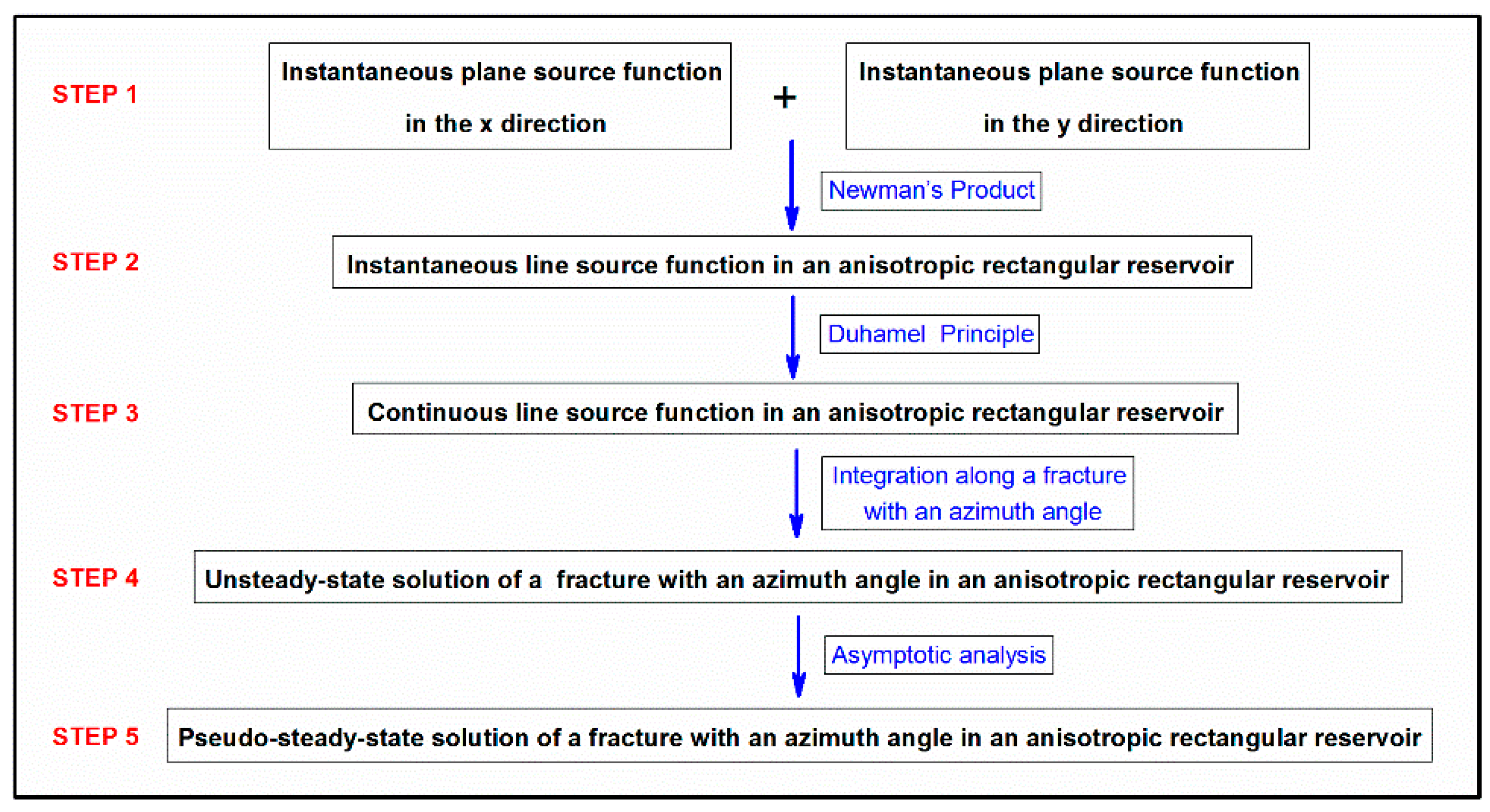
Figure 3.
Validation of a fractured well located at different positions in an anisotropic rectangular reservoir. (a) central well; (b) eccentric well.
Figure 3.
Validation of a fractured well located at different positions in an anisotropic rectangular reservoir. (a) central well; (b) eccentric well.

Figure 4.
Validation of a finite-conductivity fracture with an azimuth angle in an anisotropic reservoir.
Figure 4.
Validation of a finite-conductivity fracture with an azimuth angle in an anisotropic reservoir.
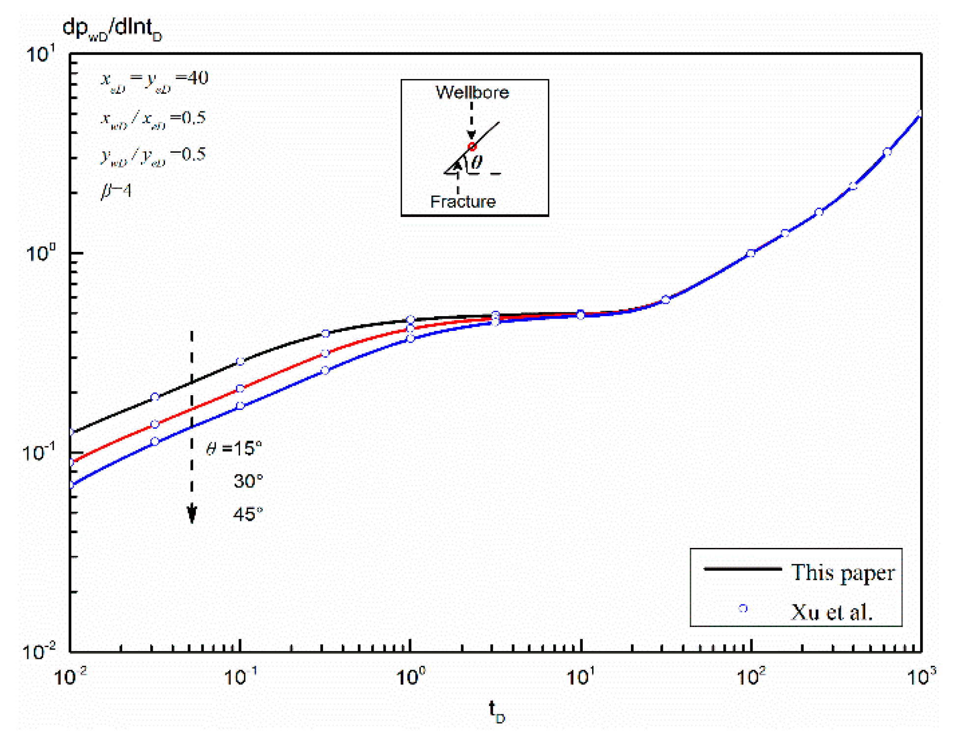
Figure 5.
Effect of permeability anisotropy on pseudo-steady-state constant: (a) ; (b)
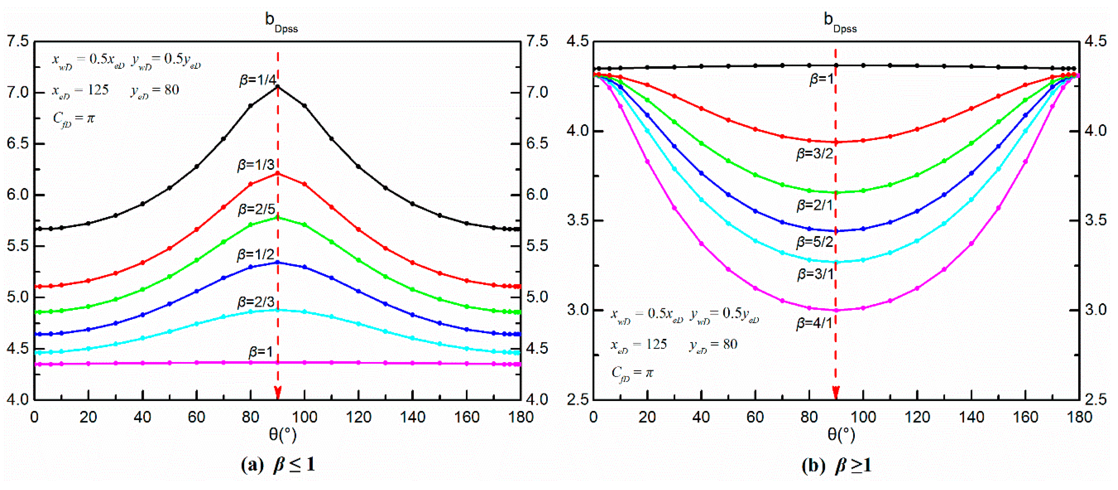
Figure 6.
Effect of permeability anisotropy on pseudo-skin factor: (a) ; (b)

Figure 7.
Effect of fracture conductivity on pseudo-steady-state constant.
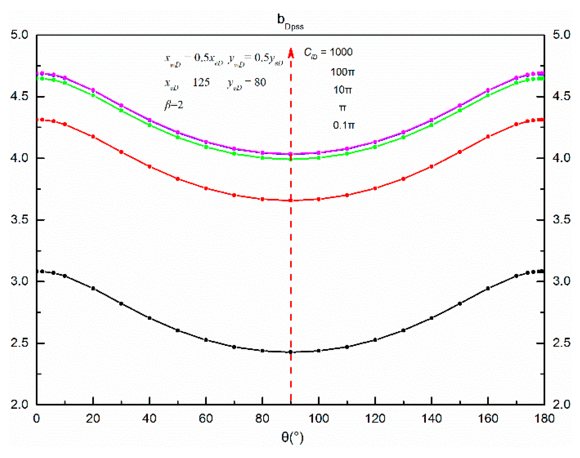
Figure 8.
Effect of fracture conductivity on pseudo-skin factor.
Figure 9.
Effect of reservoir shape on pseudo-steady-state constant: (a) ; (b) ; (c) ; (d)
Figure 10.
Effect of reservoir shape on pseudo-skin factor: (a) ; (b)
Figure 11.
Comparison of pseudo-skin factors calculated from definition and new formula.

Figure 12.
Flow regimes on Blasingame format curves for a well penetrated by a fracture with an azimuth angle in an anisotropic rectangular reservoir.
Figure 12.
Flow regimes on Blasingame format curves for a well penetrated by a fracture with an azimuth angle in an anisotropic rectangular reservoir.
Figure 13.
Blasingame format curves for a fractured well in an anisotropic rectangular reservoir at different values of azimuth angle.
Figure 13.
Blasingame format curves for a fractured well in an anisotropic rectangular reservoir at different values of azimuth angle.
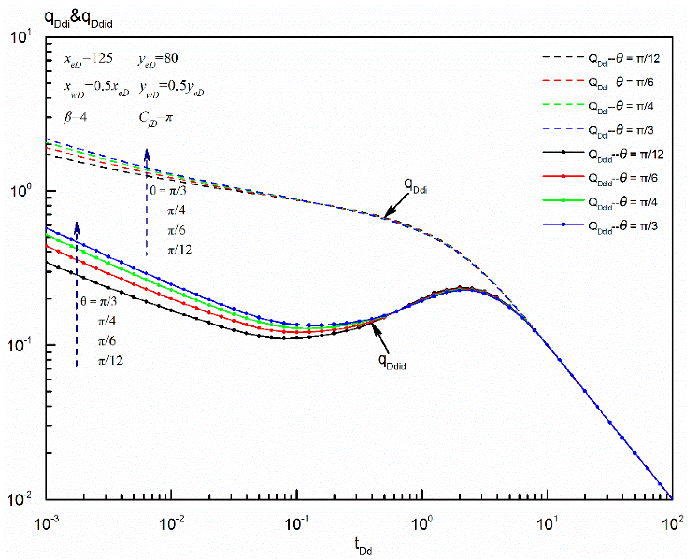
Figure 14.
Blasingame format curves for a fractured well in an anisotropic rectangular reservoir at different values of permeability anisotropy.
Figure 14.
Blasingame format curves for a fractured well in an anisotropic rectangular reservoir at different values of permeability anisotropy.

Figure 15.
Blasingame format curves for a fractured well in an anisotropic rectangular reservoir at different values of fracture conductivity.
Figure 15.
Blasingame format curves for a fractured well in an anisotropic rectangular reservoir at different values of fracture conductivity.

Figure 16.
Blasingame format curves for a fractured well in an anisotropic rectangular reservoir at different reservoir shapes.
Figure 16.
Blasingame format curves for a fractured well in an anisotropic rectangular reservoir at different reservoir shapes.


Table 1.
Dimensionless variables.
| Parameters | Definitions |
|---|---|
| Dimensionless time | |
| Dimensionless pressure | |
| Dimensionless coordinate in the x- and y-axis | , |
| Dimensionless wellbore coordinate in the x- and y-axis | , |
| Dimensionless length of the reservoir in the x axis | |
| Dimensionless width of the reservoir in the y axis | |
| Permeability anisotropic factor | |
| Dimensionless fracture conductivity | |
| Dimensionless time based on drainage area |
© 2019 by the authors. Licensee MDPI, Basel, Switzerland. This article is an open access article distributed under the terms and conditions of the Creative Commons Attribution (CC BY) license (http://creativecommons.org/licenses/by/4.0/).
Share and Cite
MDPI and ACS Style
Xing, G.; Wang, M.; Wu, S.; Li, H.; Dong, J.; Zhao, W. Pseudo-Steady-State Parameters for a Well Penetrated by a Fracture with an Azimuth Angle in an Anisotropic Reservoir. Energies 2019, 12, 2449. https://doi.org/10.3390/en12122449
AMA Style
Xing G, Wang M, Wu S, Li H, Dong J, Zhao W. Pseudo-Steady-State Parameters for a Well Penetrated by a Fracture with an Azimuth Angle in an Anisotropic Reservoir. Energies. 2019; 12(12):2449. https://doi.org/10.3390/en12122449
Chicago/Turabian StyleXing, Guoqiang, Mingxian Wang, Shuhong Wu, Hua Li, Jiangyan Dong, and Wenqi Zhao. 2019. "Pseudo-Steady-State Parameters for a Well Penetrated by a Fracture with an Azimuth Angle in an Anisotropic Reservoir" Energies 12, no. 12: 2449. https://doi.org/10.3390/en12122449
Note that from the first issue of 2016, this journal uses article numbers instead of page numbers. See further details here.