Article

Wind Power Cogeneration to Reduce Peak Electricity Demand in Mexican States Along the Gulf of Mexico

by
Quetzalcoatl Hernandez-Escobedo
1,
Javier Garrido
1,
Fernando Rueda-Martinez
1,
Gerardo Alcalá
2 and
Alberto-Jesus Perea-Moreno
3,*
1
Faculty of Engineering, Campus Coatzacoalcos, Universidad Veracruzana Mexico, Coatzacoalcos, Veracruz 96535, Mexico
2
Centro de Investigación en Recursos Energéticos y Sustentables, Universidad Veracruzana Mexico; Coatzacoalcos, Veracruz 96535, Mexico
3
Departamento de Física Aplicada, Universidad de Córdoba, ceiA3, Campus de Rabanales, 14071 Córdoba, Spain
*
Author to whom correspondence should be addressed.
Energies 2019, 12(12), 2330; https://doi.org/10.3390/en12122330
Submission received: 14 May 2019 / Revised: 7 June 2019 / Accepted: 10 June 2019 / Published: 18 June 2019
(This article belongs to the Special Issue Energy Saving at Cities)

Abstract

:
The Energetic Transition Law in Mexico has established that in the next years, the country has to produce at least 35% of its energy from clean sources in 2024. Based on this, a proposal in this study is the cogeneration between the principal thermal power plants along the Mexican states of the Gulf of Mexico with modeled wind farms near to these thermal plants with the objective to reduce peak electricity demand. These microscale models were done with hourly MERRA-2 data that included wind speed, wind direction, temperature, and atmospheric pressure with records from 1980–2018 and taking into account roughness, orography, and climatology of the site. Wind speed daily profile for each model was compared to electricity demand trajectory, and it was seen that wind speed has a peak at the same time. The amount of power delivered to the electric grid with this cogeneration in Rio Bravo and Altamira (Northeast region) is 2657.02 MW and for Tuxpan and Dos Bocas from the Eastern region is 3196.18 MW. This implies a reduction at the peak demand. In the Northeast region, the power demand at the peak is 8000 MW, and for Eastern region 7200 MW. If wind farms and thermal power plants work at the same time in Northeast and Eastern regions, the amount of power delivered by other sources of energy at this moment will be 5342.98 MW and 4003.82 MW, respectively.

1. Introduction

One of the world’s biggest problems is that population always is increasing and some countries have over dependence on energy generation. In the world, primary energy consumption growth averaged 2.2% in 2017, up from 1.2% last year and the fastest since 2013. This compares with the 10-year average of 1.7% per year [1]. In 2016, generation from combustible fuels accounted for 67.3% of total world gross electricity production (of which: 65.1% from fossil fuels; 2.3% from biofuels and waste), hydroelectric plants (including pumped storage) provided 16.6%; nuclear plants 10.4%; geothermal, solar, wind, tide, and other sources 5.6%; and biofuels and waste made up the remaining 2.3% [2]. It is known that energy supply side and demand side is essential to the correct usage of energy [3], and this is important to nations because it depends on the effectiveness of its power systems and the availability of power supply at the load centers [4]. It is important to define the concepts of load and electricity demand, on the one hand to understanding load of an electric power distribution as the final stage of the system that converts electric energy in another form of energy; respecting electricity demand is known as the electric power related on a period of time, that uses load to work.
In Mexico, electricity demand is considered decisive in social and economic development and consequently in the improvement of the economic conditions. The maximum demand for electrical energy occurs mainly during the summer season, between May and September, when the heat is more severe in the north and southeast of the country. As a result, the use of ventilation equipment is increased to maintain the temperature at more comfortable levels and the values necessary for the proper functioning of certain appliances are regulated. In 2017, the energy independence index, which shows the relationship between production and national energy consumption, was equivalent to 0.76. This result implies that the amount of energy produced in the country was 24.0% less than that which was made available in the various consumer activities in the national territory. In the course of the last ten years, this indicator decreased in an average annual rate of 5.0% [5]. An alternative will be the use of renewable energy, the Transition Energetic Law establish a renewable energy minimal participation in electricity generation of 25%, 30% and 35% in 2018, 2021, and 2024, respectively [6]. In the energetic mix, renewable energies have a participation of 14%, the technologies most used are hydraulic, and wind energy contributed with 3% or 38.23 PJ in 2017 [7].
Peak electricity demand is a global policy concern which creates transmission constraints and congestion, and raises the cost of electricity for all end-users [8]. Also, a considerable investment is required to upgrade electricity distribution and transmission infrastructure, and build generation plants to provide power during peak demand periods [9]. This is important because usually service suppliers charge a higher price for services at peak-time than for off-peak time to compensate for the costly electricity generation at peak hours [10]. Thus, if peak demand is reduced, electric system will be benefited. In addition to these benefits a study done by the authors of Reference [11] determine that it can eliminate the need to install expensive extra generation capacity such as combustion turbines for peak hours which are less than a hundred hours a year. With this information regions will be considered where demand complies with the conditions to have the necessary hours. Another benefit is for consumers, because if they know the period of time of peak demand and decrease their consumption, they can avoid higher electricity prices. An option to reduce peak demand is installing peak plants but the economic benefit does not justify the investment. Usually these peak plants use fossil fuel and the result is more generation of greenhouse gases [12].
The use of wind energy to support the electric demand mainly during its peak period is an alternative to reduce fossil fuel combustion and greenhouse gas emissions. Wind is intermittent and uncertain, which represents a problem in power systems [13]. A study done by the authors of Reference [14] established that due to the unpredictable nature of wind energy and non-coincidence between wind units output power and demand peak load, wind units are deemed as an unreliable source of energy. In this study a stochastic mathematical model was developed for the optimal allocation of energy storage units in active distribution networks in order to reduce wind power spillage and load curtailment while managing congestion and voltage deviation.
In New York State the intraregional effects were illustrated by quantifying the net load, net load ramping, operating reserve, and regulation requirements, the study found out that only at wind capacities exceeding 100% of the average statewide load does the wind-generated electricity meet significant portions of the distant demands [15].
An improved energy hub system combined with cooling, heating, and power integrated with photovoltaic and wind turbine, demonstrated that operation cost and carbon emission were reduced by 3.9% and 2.26%, respectively [16]. In Canada a battery storage system to minimize the energy drawn from the public grid was proposed This storage system was charged from wind turbines and the energy stores were discharged to a park when the wind park power dropped below 0 kW and the storage system was able to offset 17.2 MWh but the financial gain was insufficient to offset the net energy losses in the storage system [17].
About cogeneration, in China Reference [18] established the relationship between a wind farm and a thermal power plant, in this study the difference between wind power profits and thermal power is only analyzed in terms of cost differences, and no comparison of other data is involved. According to this, the specific example of Gansu Province not only shows the difference in earnings before and after the peak-to-peak adjustment of wind power, but also indicates that the large-scale auxiliary adjustment of wind power can ensure that thermal power generators can participate in deep-peaking with reasonable returns; Reference [19] analyses and compares several existing kinds of distributed energy storage for improving wind power integration. Then considering a mass of cogeneration units in north China, control strategy for wind power integration is proposed to reduce the peak regulation capacity for wind power integration. As a result, the peak–valley load difference can be equivalently reduced to relieve peaking pressure for wind power integration.
In Northern China a proposal were made suggesting that if the energy carrier for part of the end users space heating is switched from heating water to electricity (e.g., electric heat pumps can provide space heating in the domestic sector), the ratio of electricity to heating water load should be adjusted to optimize the power dispatch between cogeneration units and wind turbines, resulting in fuel conservation, they found out that with the existing infrastructures are made full use of, and no additional ones are required [20]. Bexten et al. [21] investigate a system configuration, which incorporates a heat-driven industrial gas turbine interacting with a wind farm providing volatile renewable power generation. The study quantifies the impact of selected system design parameters on the quality of local wind power system integration that can be achieved with a specific set of parameters. Results show that the investigated system configuration has the ability to significantly increase the level of local wind power integration.
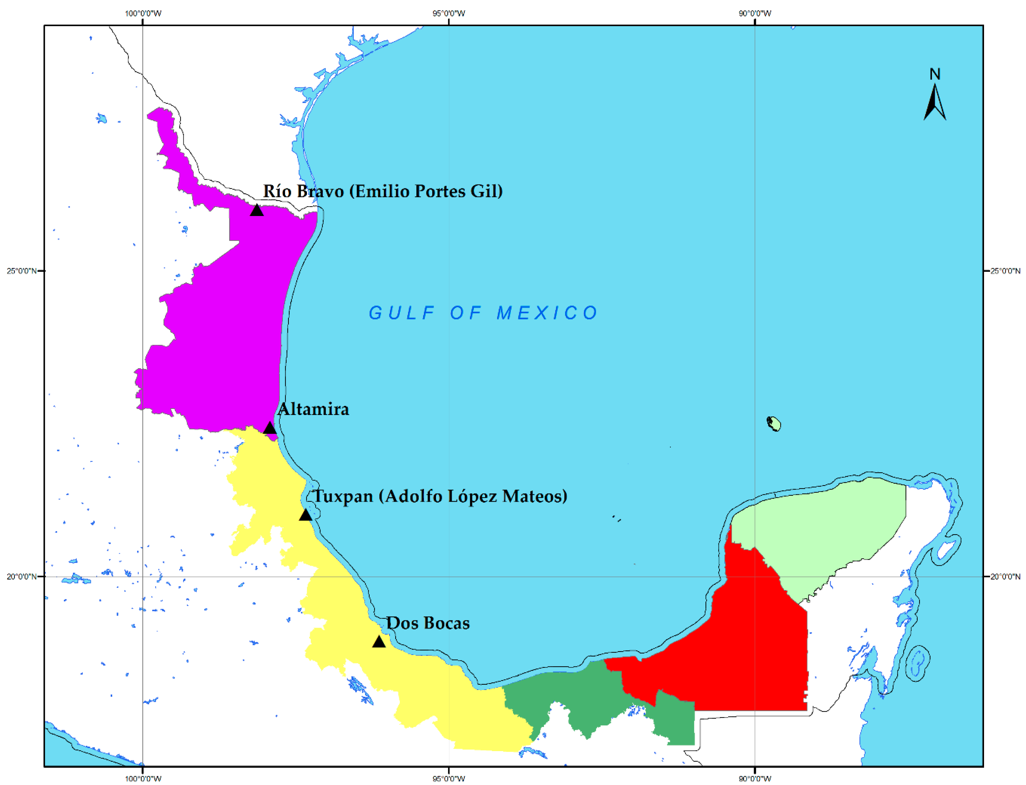
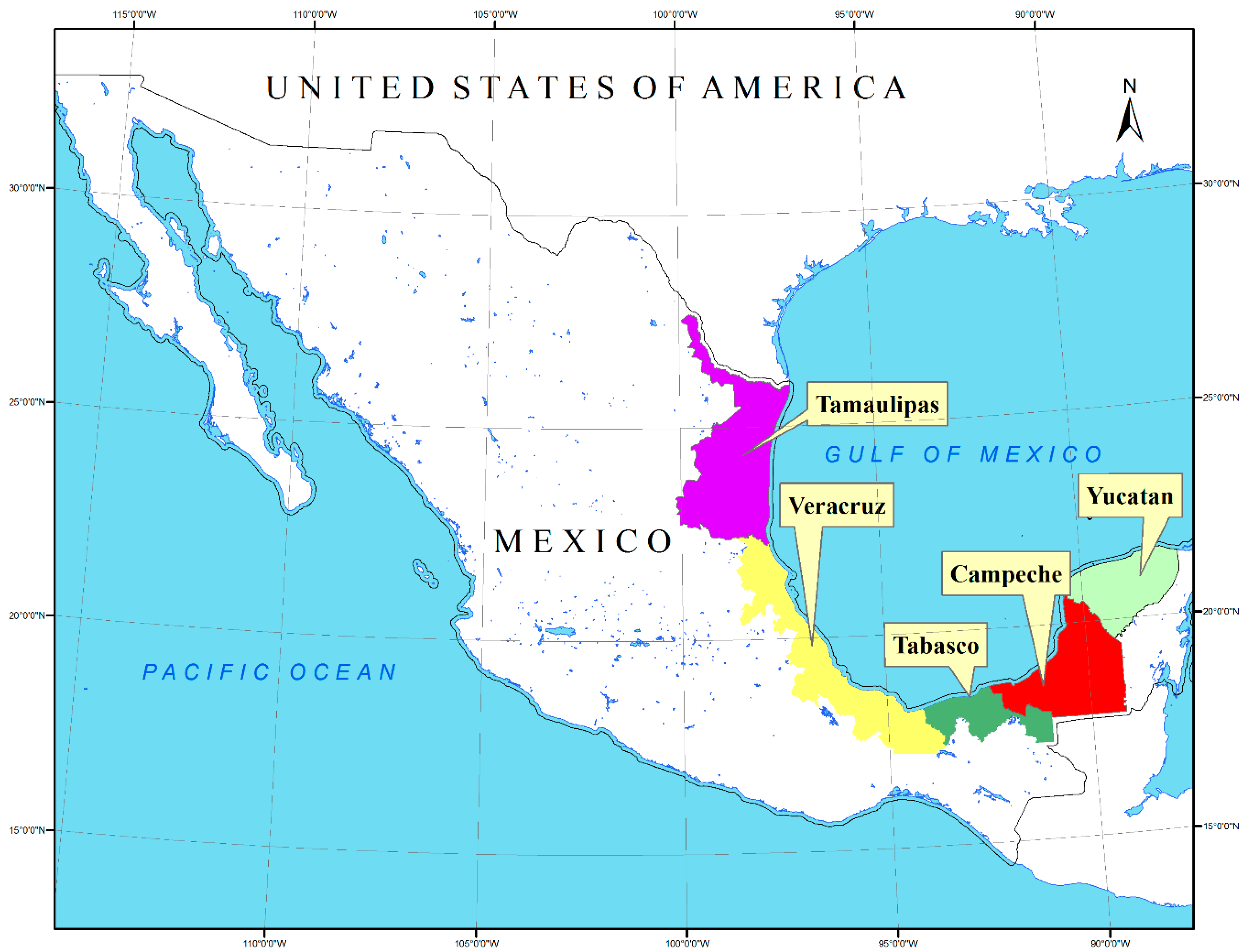
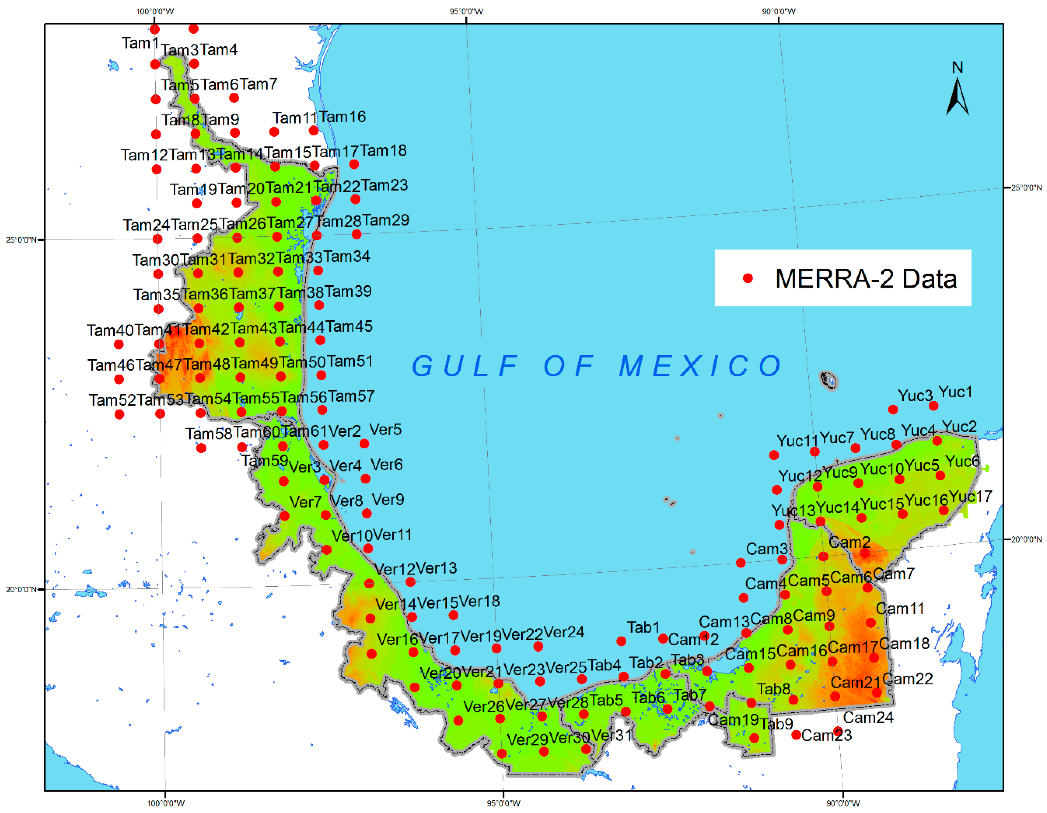
In this study a methodology is proposed, which consists in locating thermal power plants along the five states of the Gulf of Mexico (Tamaulipas, Veracruz, Tabasco, Campeche, and Yucatan) and evaluating wind resources next to these plants with the objective to determine the power output generated and their contribution to reduce the peak electricity demand. For the geographic position of Mexican states along the Gulf of Mexico, see Figure 1.

2. Material and Methods

2.1. Data

Modern-Era Retrospective analysis for Research and Applications, Version 2 (MERRA-2) provides re-analysis data such as: wind speed and wind direction at 50 m height, temperature at 2 m and 10 m, and atmospheric pressure with records from 1980–2018. The resolution of every point downloaded is 50 km covering all the Mexican states along the Gulf of Mexico including offshore points, which can all be observed in Figure 2. Several studies have used MERRA-2 to determine wind characteristics, as did Reference [22] in the Central Californian Coast, assessing offshore conditions. A study about wind and rainfall areas of tropical cyclones making landfall over South Korea was examined for the period 1998–2013 using MERRA-2 data. It was determined that composite analyses of the cases of strong and weak vertical wind shear confirm that the increase of rainfall area is related to the asymmetric convection (rising/sinking motion in the downshear-left/upshear-right side) induced by the vertical wind shear [23]. An investigation on prediction of wind power because of climate change was made using MERRA-2 among other re-analysis data [24]. As can be seen, MERRA-2 data have been used with excellent results on wind assessment.
In total, 142 MERRA-2 points, 61 in Tamaulipas, 31 in Veracruz, 9 in Tabasco, 24 in Campeche and 17 in Yucatan.

2.2. Thermal Power Plants

There are 22 thermal power plants in Mexico that generate electricity. These plants work on a combined cycle with gas turbines. This generation contributes 55.6% of all electricity in the country [25]. Along the Gulf of Mexico, the most important plants are located as follows: two in the state of Veracruz, one called Adolfo Lopez Mateos with capacity of 2263 MW and Dos Bocas with capacity 350 MW. In the state of Tamaulipas there are two, Rio Bravo and Altamira, with capacity of 800 MW and 1039 MW respectively [26]. Figure 3 shows the geographic position of these thermal power plants. Unfortunately, there are no thermal plants located in the states of Tabasco, Campeche, and Yucatan.

2.3. Wind Assessment

Wind characterization is essential to determine its power at a given site. Its assessment depends mainly on the orography, roughness, and generalized climatology.
Statistically it can be characterized as a probability density function (PDF) that can be interpreted as the probability that the random variable x lies in a differential range, dx, about a value x is f(x)dx. More specific statements about the probability that the unsteady variable x, lies in a particular range axb, this expression is given by Equation (1).
P = ( a x b ) = a b f ( x ) d x ,
Another PDF used in wind assessment is the Weibull distribution for the wind speed (u) that has two parameters: shape parameter (k) and scale parameter (c). This is expressed in Equation (2):
f ( u ) = k c ( u c ) k 1 e ( u c ) k ,
The power in the wind is the product of mass flow rate through turbine blades ρUA, and the kinetic energy per unit mass in the wind, U2/2. The average power in the incoming wind is presented in Equation (3) [27].
P = 1 2 ρ A U 3 C P ,
where ρ is the density of air, CP is the power coefficient, A is the rotor swept area, U is the wind speed and P is the wind turbine power output.

2.4. Peak Electrical Demand

In Mexico the National Energy Control Center (NECC) divided the country in seven regions. This division is called National Interconnected System [28], and is based in two electric regions: Northeast and Eastern [29]. These regions can be seen in Figure 4.
NECC shows information about demand forecasting, net demand, and total demand. It uses three methodologies to calculate demand forecasting: moving average that is optimal for random or leveled demand patterns where the impact of historical irregular elements is to be eliminated through an approach of periods of up to 7 days previously. This methodology is the most used by NECC and is given by Equation (4)
X ^ t = i = 1 n x t 1 n ,
where X ^ t is the energy demand average in period t; X t 1 is the real demand for the periods prior to t and the number of observations n.
The second method is weighted moving average, a variation of moving average. While in moving average all data has the same weight, in weighted moving average each data is assigned with a specific weight, always considering that total sum will be 100% and is expressed as Equation (5):
X ^ t = i = 1 n c i x t 1 ,
where X ^ t is the energy demand average in period t; c i weighted factor; x t 1 is the real demand for the periods prior to t and the number of observations n.
The third method is called multiple linear regression, where both independent and dependent variables working with the independent variable variation to forecasting the dependent variable. Multiple linear regression is given by Equation (6):
D F = β 0 + β 1 x 1 + + β n x n + ε ,
where DF is Demand Forecasted; x1, …xn independent variables; β0βn coefficients which are calculated by least squares; n number of data and ε is a random error term.
Several studies about peak demand where demand consumers participate have established two typical types of programs. The first one is an incentive-based program the end users are encouraged by the incentive payments to reduce their load demands, and thus to help improve the feasibility and stability of the power system [30]. This program usually includes direct load control and demand bidding [31]. The second one is price-based, and in this case final consumers are encouraged to configure their energy usage patterns according to electricity demand curve. These price-based programs consist in observing critical peaking pricing, time of use pricing, and time pricing [32,33].
Figure 5 presents two demand curves, each one by region. These demand curves have been developed with the aim to estimate the current hourly electricity demand profiles with a temporal resolution of 1 h based in 2018.
As seen in Figure 5, the behavior of electric demand varies among regions, Figure 5a at Northeast the peak appears in range of 16:00–18:00 h and has another peak during 22:00–24:00 h. This is because the consumption increases in the first peak due to domestic use and the second electricity peak is due to industrial sector and in Figure 5b the Eastern region presents a peak demand during 21:00–23:00 h, mainly for industrial activities.
These demand curves will be used and compared to wind daily profile to consider it as wind power.

3. Results and Discussion

Along the Gulf of Mexico 142 MERRA-2 points have been assessed with wind speed information. 4 sites around thermal power plants have been chosen and the amount of power output generated has been calculated to reduce peak electricity demand.

3.1. Wind Resource Assessment

Wind has been converted as resource along the Gulf of Mexico; this means that mainly both roughness and orography have been taken into account.

3.1.1. Rio Bravo, Altamira, Tuxpan, and Dos Bocas

Four MERRA-2 points were located near thermal power plants, their geographic information is presented in Table 1.
In Appendix A Table A1, Table A2, Table A3 and Table A4 hourly mean wind speed are presented by month for MERRA-2 points. In each one of them wind speed behavior can be appreciated.
A typical wind year can be compared to electricity demand to identify its trajectory, so that it could be seen if in the peak demand there existed a peak wind. To probe it, Figure 6 and Figure 7 represent both electricity demand and wind speed of Rio Bravo, Altamira, Tuxpan, and Dos Bocas respectively.
As can be observed in Figure 6, wind speed trajectory has an increase in the last hours as the electricity demand does as follows: Figure 6a 6.8 m/s to 7.6 m/s and Figure 6b 5 m/s to 6.5 m/s both during 21:00 h to 24:00 h. Although Figure 6b does not follow the entire trajectory, at the end of the day the last 4 h (21:00–24:00) when the demand begins to grow, wind also does. In Figure 7a 4.5 m/s to 6.5 m/s and Figure 7b 5 m/s to 6 m/s both between 20:00 h to 24:00 h. This could be considered to model a potential source of power.
Determining wind speed features correctly means that the model that will be designed will have more accuracy. In Table 2, statistical information at the points studied is presented.

3.1.2. Microscale Model

One of the critical criteria to place wind turbines is to assess wind resource and determine if the site have features as transmission lines, substations, and roads, among others.
A microscale model has been done on WAsP software including roughness and orography features. In Figure 8 and Figure 9 the four sites are shown microscale modeled. Each one has an array of seven wind turbines placed to avoid wake effect. Wind turbines generators (WTG) are selected according to wind features at the site.
Modeled areas show different types of wind resource, and the resolution is 10 km. The areas of high wind energy potential are better identified. An advantage of microscale modelling is to extrapolate onsite measurements to the prospective turbine sites to modify the background atmospheric conditions and account for topographic induced speedups, turbulence, and wind shear [34]. The x and y axes are represented in UTM scale, in Figure 8a the zone presents a wind power density between 261 W/m2 to 286 W/m2, WTG type GEWind 77 were placed to avoid wake effects; Figure 8b presents a zone with 170 W/m2, level curves show hills in this area and were harnessed to place WTG type BONUS 600 kW along it. In Figure 9a, this zone is in front of the sea, an area with 142 W/m2, wind turbines VESTAS V82-1650 kW were used; Figure 9b. In Dos Bocas there is a wind power density of 144 W/m2. Seven WTC type BONUS 600 kW were placed at the top of the hills.

3.1.3. Power Output Generation and Electricity Peak Demand

In the northeast region, peak demand occurs twice per day, the first period at 17:00 h and the second one at 24:00 h. These peaks represent a higher price of electricity by consumers. Wind speed at Rio Bravo behaves similarly to electricity demand curve, wind daily profile has two peaks, and these at the same time. Meanwhile, wind speed profile in Altamira only has one peak at the end of the day, even so power can be extracted from the wind. The power contribution by two wind farms placed in Rio Bravo and Altamira in the state of Tamaulipas, respectively, is shown in Table 3.
In the state of Veracruz located at the eastern electricity region, wind has been analyzed near two thermal power plants. In this region, electricity demand has a peak that occurs at 22:00 h in both Tuxpan and Dos Bocas, and wind speed trajectory shows that it can contribute delivering electricity to the grid at the same time that peak demand occurs. Table 4 presents the power output generated of two wind farms at the state of Veracruz.
If the period of time and the wind speed are taken into account when peak demand is increasing, it will be able to calculate how much energy could be extracted in each point, see Table 5.
As shown in Table 5, electric power generated by each wind farm could contribute to reduce peak demand. The electric power generated by region indicate an amount of 2657.02 MW for Northeast and 3196.18 MW for Eastern. This is the power delivered to the electric grid.
Wind resource assessment is fundamental to determine the site where wind can be used to generated electric power. Another variable that can be considered is the place, which is important taking into account electricity required, as mentioned in Reference [9]. In this work, wind farms were modeled near to thermal power plants and used their electric infrastructure. It was found the hours at day were both electricity demand and wind speed have their peaks, whit this information could benefit end-users as studied [12] that establish if consumers know the period of time were peak demand occurs could avoid higher electricity prices. This work presents a methodology to assess wind speed and calculate the power delivered to the grid, but is important to mention that if only wind speed is assessed and other variables such as roughness, orography, and climatology are not considered, wind cannot be considered as an unreliable source, as did Reference [15]. To avoid this problem, a proposal of cogeneration with thermal power plants has been made, in comparison with Reference [18] where a cost analysis was its main objective, we have analyzed wind data trajectory to reduce peak demand.
The proposal of connection to the power grid is based on the thermal power plant of Dos Bocas. The same connection is considered for the other thermal plants. In this case, the nominal power, that is, 350 MW, and the wind farm nominal power of 10.5 MW, is equivalent to 3% of the total substation capacity which indicates that the connection is possible. For Rio Bravo 800 MW, the connection will represent 1.3%, Altamira 1039 MW will be 1%, and Tuxpan 2263 MW. This connection represents 0.4% of the substation capacity.
Regarding the impact of new wind farms on power grids, Reference [35] established that power losses in distribution systems vary with numerous factors depending on the system configuration, such as level of losses through transmission and distribution lines, transformers, capacitors, and insulator, among others. In the case of this study, all the power losses were calculated in the original design. Appendix B shows a single line diagram where the transmission lines and the node modified with the connected wind farm can be seen.

4. Conclusions

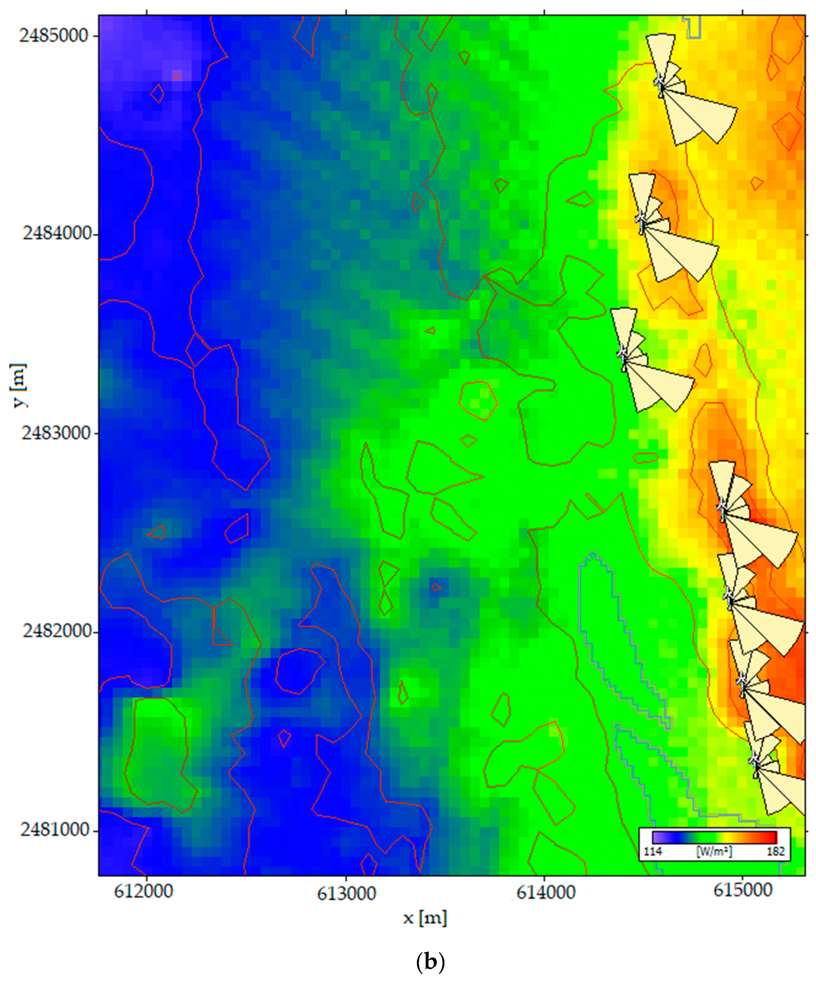
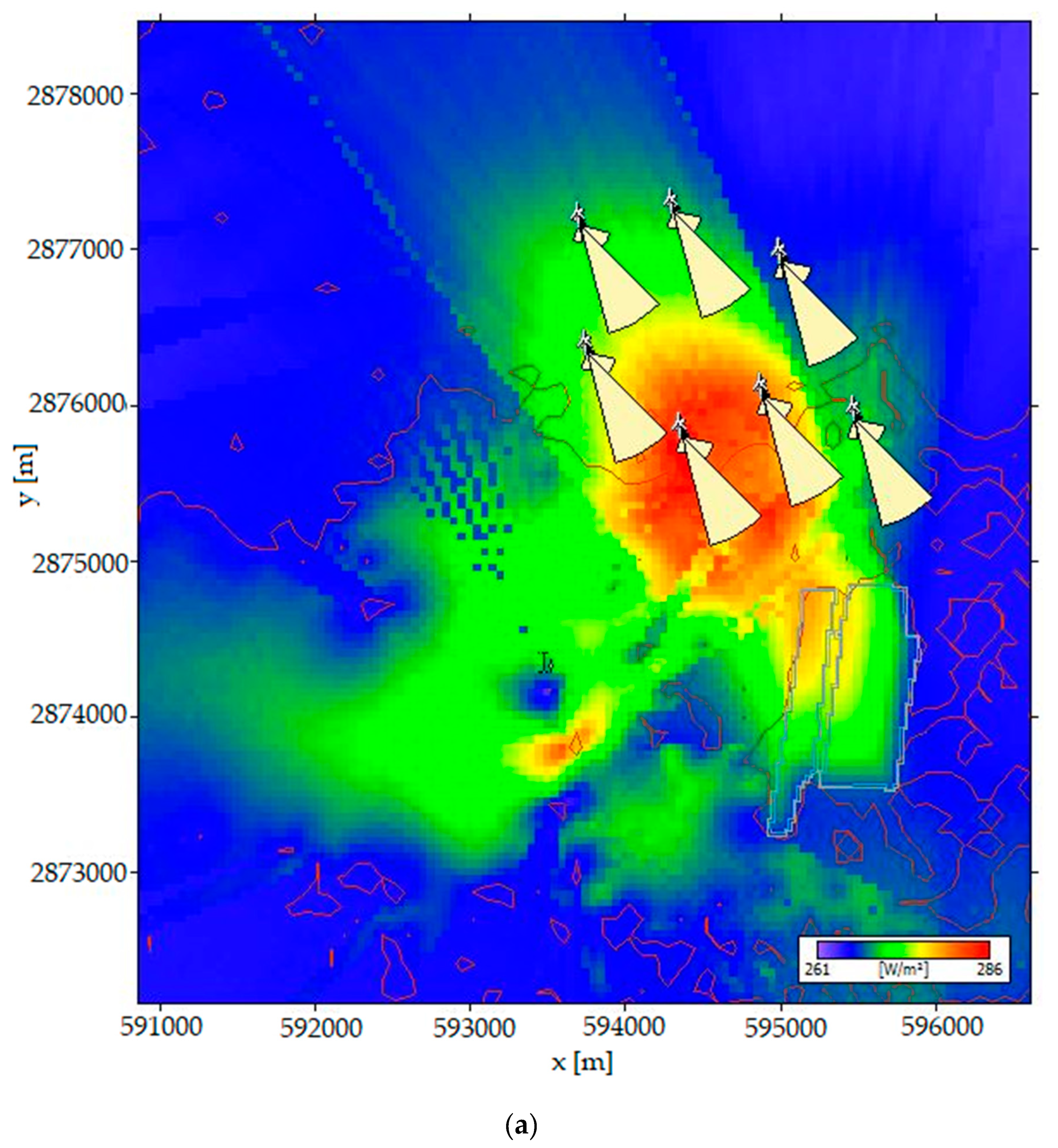
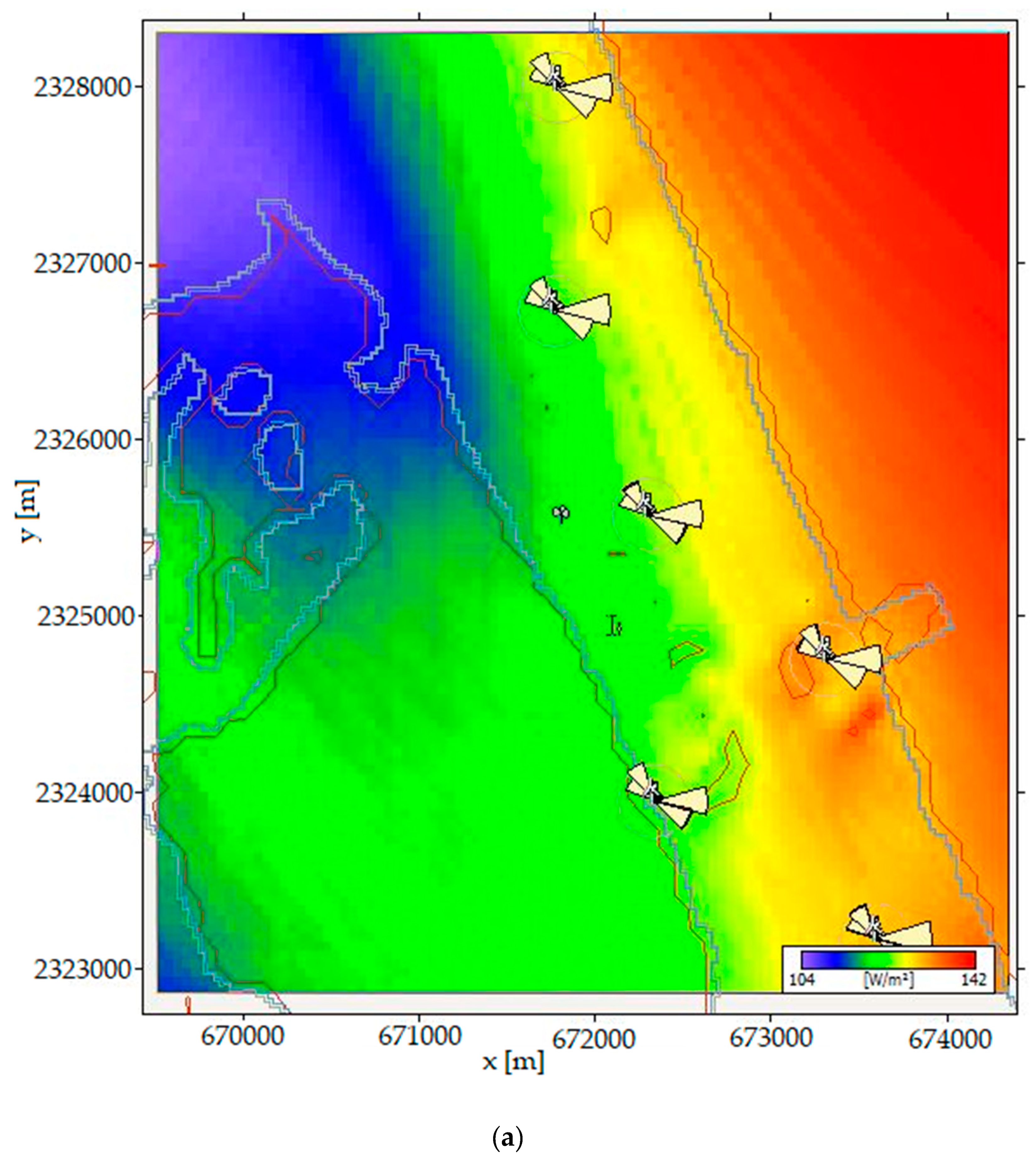
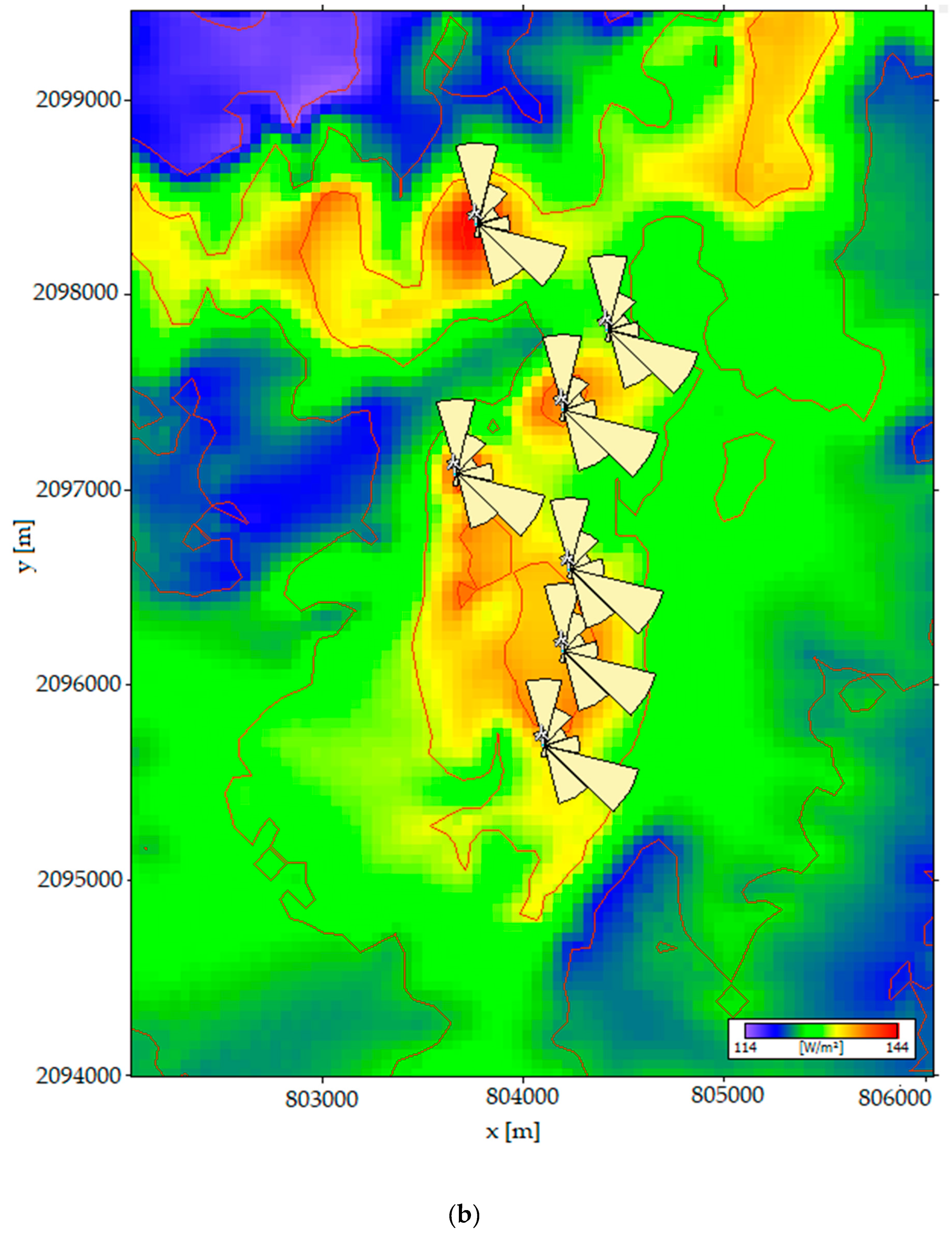
The microscale model increased the accuracy of wind assessment to place wind farms. This is because when running the microscale model, several variables are taken into account such as roughness, orography, and climatology. In this study, four sites were assessed to model wind farms using MERRA-2 data, wind speed, wind direction, temperature, and atmospheric pressure, with records from 1980–2018.
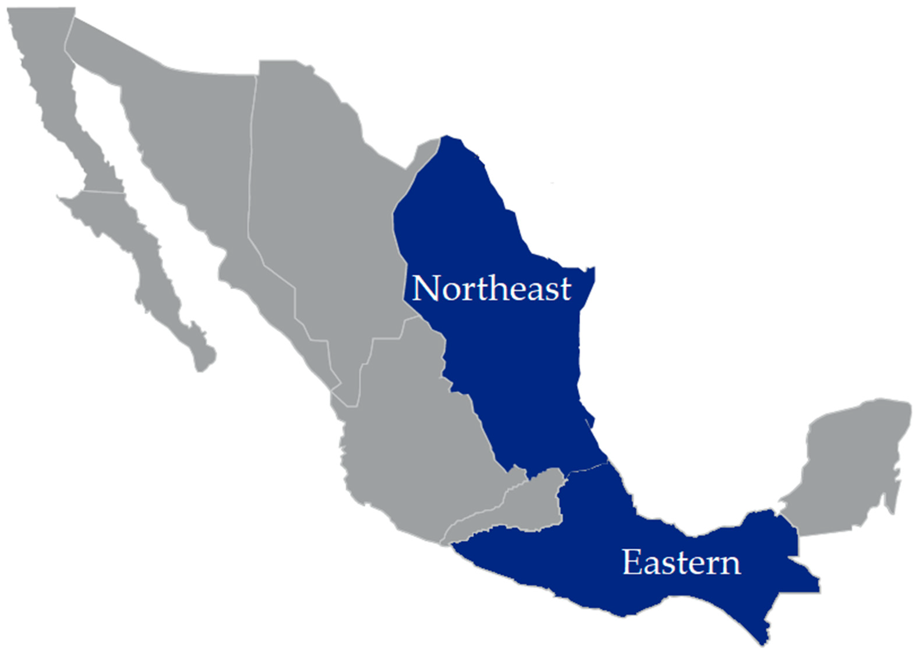
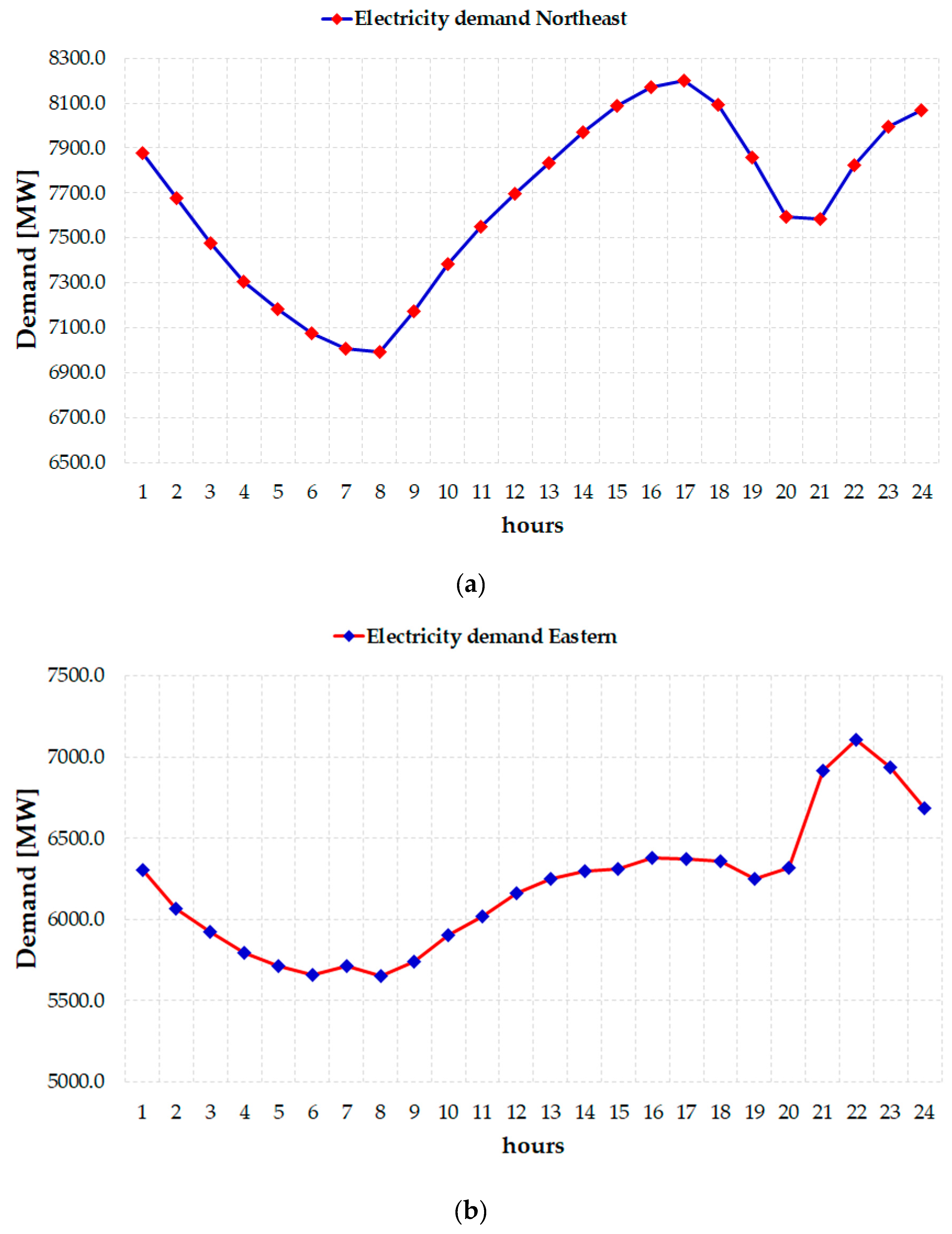
The electricity that wind farms generate is delivered over transmission and distribution power lines. High-voltage transmission lines carry electricity over long distances to where consumers need it. More distance means more losses. The amount of power produced by each wind farm could contribute to the power produced by a thermal plant. In total for Northeast region they can deliver to the grid 2657.02 MW at peak demand. If there is 8000 MW demanded at this moment, the reduction will be at 5342.98 MW. At the Eastern region, the thermal power plant called Tuxpan is the biggest one in Mexico, so the amount of power in both wind farms and thermal plants is higher than Northeast. In this case, the total production is 3196.18 MW, and peak demand power delivered is 7200 MW if wind farms and thermal power plants work at the same time. The amount of power at this moment will be 4003.82 MW. There could be several techniques to contribute to decreased peak demand, energy storage technologies, and faster response times, but the most important is to nurture future generations.
The impact of the thermal power plants, once they have the contribution of wind energy, can be considered as follows: the efficiency for Rio Bravo and Altamira could be 31% and for Tuxpan and Dos Bocas 47%; the capacity factor, 36% and 56% respectively, however, the volatility and availability of wind in the entire year must be considered.
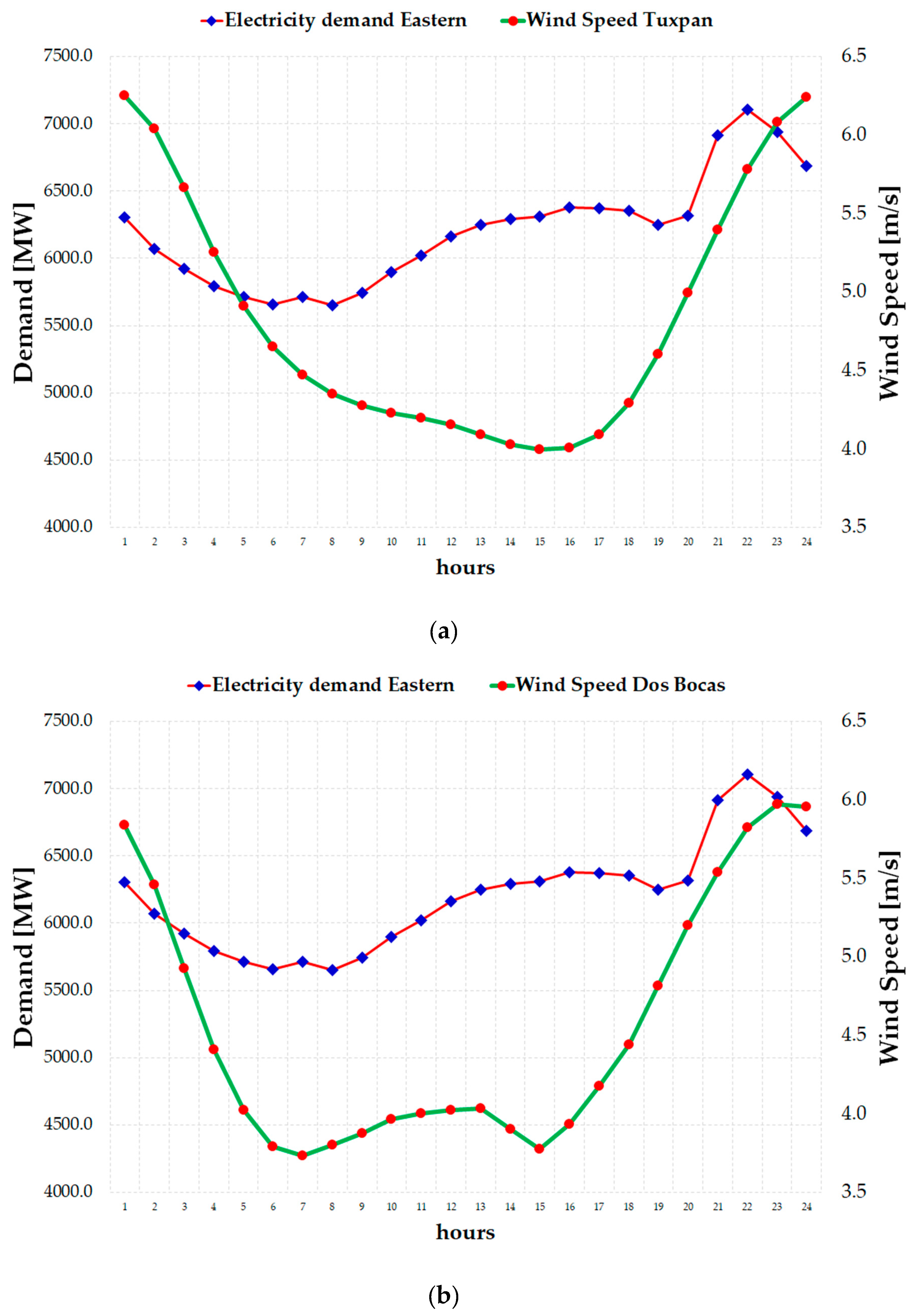
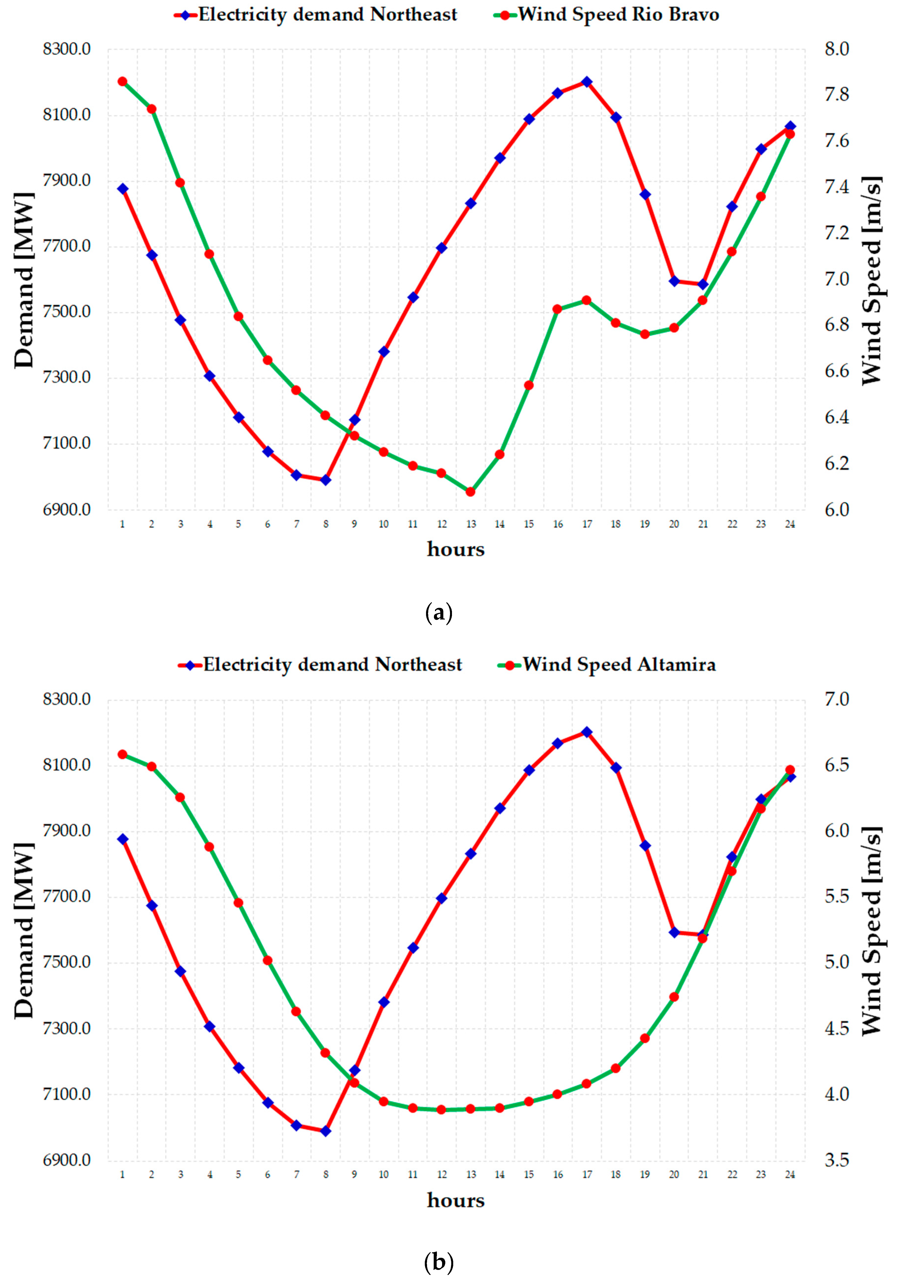
Mexico’s main objective is to reach 35% of its electricity generated by clean sources in 2024. Employing this type of generation is important to contemplate both the trajectory of electricity demand and wind speed and to avoid a duck-curve that represents several renewable sources being contributed during the day but not at night, as solar or when wind does not has enough potential, e.g., Northeast curve has two peaks during the day, the first one peak is at 17:00 h and the second one is at 24:00 h, at this hour solar energy cannot be consider and if at this time does not flow the wind, the peak demand will increase and the prices will also do it.

Author Contributions

Q.H.-E. and A.-J.P.-M. have contributed to the theoretical approaches, simulation, experimental tests, and preparation of the article, and have contributed equally to this work. J.G., F.R.-M. and G.A. All authors have read and approved the final manuscript.

Funding

This research was funded by Ministry of Education Mexico, under the project Support to Research Groups, UV-CA-466.

Acknowledgments

Authors acknowledge to research group “Wind and solar energy” from Universidad del Istmo.

Conflicts of Interest

The authors declare no conflict of interest.

Appendix A

Table A1. Hourly mean wind speed in Rio Bravo Mexico.
HourWind Speed [m/s]
JanFebMarAprMayJunJulAugSepOctNovDec
0:007.17.78.48.58.68.68.88.27.17.37.26.9
1:007.27.88.38.38.38.38.47.87.07.37.37.0
2:007.17.68.07.97.87.87.87.36.67.07.16.9
3:006.97.37.77.67.47.47.46.96.36.76.96.8
4:006.87.17.47.37.27.17.16.55.96.46.86.7
5:006.67.07.27.27.16.86.86.25.66.26.66.6
6:006.67.07.17.17.06.66.65.95.36.06.56.5
7:006.56.97.17.16.96.46.45.65.15.96.56.5
8:006.56.97.17.06.96.36.25.34.95.86.56.4
9:006.56.97.17.06.86.16.05.14.85.76.56.5
10:006.66.97.17.06.86.05.85.04.85.66.56.5
11:006.66.97.17.06.85.95.74.94.75.66.46.5
12:006.66.97.16.96.65.75.54.74.75.66.46.4
13:006.56.76.87.17.36.66.45.24.55.36.36.4
14:006.16.77.67.87.86.97.15.95.15.66.05.9
15:006.67.48.07.97.86.97.15.95.36.26.86.5
16:007.07.47.97.77.66.77.15.95.46.27.07.0
17:007.07.27.77.57.46.77.15.95.46.16.96.9
18:006.87.07.57.37.36.87.26.15.66.16.76.7
19:006.76.97.47.37.37.17.56.55.86.16.56.5
20:006.66.87.47.47.57.47.96.96.16.36.56.4
21:006.56.97.57.67.87.88.37.36.46.56.56.4
22:006.57.17.87.98.18.28.67.86.76.86.66.3
23:006.77.48.18.38.58.58.88.16.97.06.86.5
Table A2. Hourly mean wind speed in Altamira Mexico.
HourWind Speed [m/s]
JanFebMarAprMayJunJulAugSepOctNovDec
0:006.77.18.08.07.26.35.75.45.76.16.36.5
1:006.77.17.77.67.06.25.75.45.66.16.36.5
2:006.56.87.27.16.76.15.55.25.55.96.26.4
3:006.16.36.66.56.35.85.35.05.15.65.96.1
4:005.75.86.05.85.75.55.14.74.75.35.55.7
5:005.35.35.45.25.15.14.84.34.34.95.25.3
6:005.04.94.94.74.64.74.43.94.04.64.95.0
7:004.84.64.64.34.24.24.03.53.74.34.74.9
8:004.74.44.34.13.93.83.63.23.54.24.64.8
9:004.74.44.13.93.73.53.32.93.54.14.54.8
10:004.74.44.13.93.63.33.12.83.54.14.54.8
11:004.84.44.13.93.53.23.02.73.54.14.64.8
12:004.84.54.13.93.53.12.92.73.64.24.64.8
13:004.94.54.23.93.63.12.82.63.54.24.74.8
14:004.84.64.34.13.83.22.92.73.54.14.64.8
15:004.84.74.54.23.93.33.02.73.54.14.64.7
16:004.84.74.64.44.13.43.12.83.64.14.74.7
17:004.84.74.84.64.43.73.42.93.74.14.64.7
18:004.84.85.05.14.94.13.73.33.94.34.64.6
19:004.85.15.55.65.34.54.23.74.34.54.74.7
20:005.15.56.16.35.95.04.74.24.74.85.04.9
21:005.56.16.97.16.45.55.24.75.15.25.45.3
22:006.16.77.67.76.95.95.55.15.45.65.85.8
23:006.47.18.08.17.16.25.75.35.65.96.16.1
Table A3. Hourly mean wind speed in Tuxpan Mexico.
HourWind Speed [m/s]
JanFebMarAprMayJunJulAugSepOctNovDec
0:006.06.57.07.27.26.66.05.65.55.85.95.9
1:005.86.26.56.76.86.45.95.55.55.75.85.7
2:005.45.75.96.16.25.95.65.25.35.55.65.5
3:005.15.25.45.55.75.55.34.94.95.25.35.2
4:004.94.95.15.15.25.04.94.44.54.85.05.0
5:004.94.84.94.94.84.54.53.94.24.64.95.0
6:004.94.74.84.74.54.14.13.64.04.54.84.9
7:004.94.74.64.54.33.83.83.43.94.54.84.9
8:004.94.74.64.44.23.63.63.23.94.54.84.9
9:004.94.74.64.44.13.43.43.14.04.64.84.9
10:004.94.74.64.44.03.33.23.04.04.64.84.9
11:004.94.74.54.33.93.23.13.04.04.74.84.9
12:004.94.74.54.23.73.13.03.04.04.64.84.9
13:004.94.54.34.13.73.13.02.93.94.54.74.8
14:004.74.54.44.13.73.23.12.93.84.34.64.7
15:004.74.64.44.13.73.23.12.83.74.34.64.7
16:004.84.74.64.33.83.43.32.93.84.34.64.7
17:004.84.84.84.74.23.83.63.23.94.44.74.7
18:004.95.05.25.14.84.44.13.64.14.54.84.8
19:005.15.45.75.75.45.14.64.14.44.74.94.9
20:005.35.76.26.36.05.75.24.64.74.95.15.1
21:005.66.06.76.86.56.25.65.05.15.25.35.3
22:005.86.47.07.26.96.55.95.45.45.55.65.5
23:005.96.57.27.37.26.76.05.55.55.65.75.7
Table A4. Hourly mean wind speed in Dos Bocas Mexico.
HourWind Speed [m/s]
JanFebMarAprMayJunJulAugSepOctNovDec
0:006.36.56.86.76.35.44.44.45.16.06.16.1
1:005.85.85.95.85.75.14.34.45.15.95.95.8
2:005.25.04.94.84.74.74.14.15.05.75.65.3
3:004.74.44.13.93.94.23.83.84.75.45.24.8
4:004.44.13.73.43.23.73.43.44.45.14.94.6
5:004.34.03.63.22.93.33.13.14.14.84.74.4
6:004.34.03.63.22.83.13.13.13.94.74.64.4
7:004.44.13.83.32.83.13.23.13.94.74.74.5
8:004.54.24.03.42.93.13.43.33.84.74.74.5
9:004.64.34.13.63.03.13.53.43.94.74.84.6
10:004.64.44.13.73.03.13.63.53.94.74.84.6
11:004.64.44.13.73.13.13.73.63.94.74.84.6
12:004.64.44.13.73.13.13.73.73.94.74.84.6
13:004.54.34.03.73.12.93.23.43.84.64.74.6
14:004.34.44.24.03.32.82.62.83.54.54.64.3
15:004.64.74.54.23.63.02.52.63.54.74.84.5
16:004.85.04.84.64.03.32.62.73.74.95.04.7
17:005.15.25.15.04.43.62.92.93.95.15.24.9
18:005.45.55.65.55.04.13.33.34.35.35.45.1
19:005.75.96.16.15.54.53.73.64.65.65.75.4
20:006.06.36.66.66.04.94.03.94.95.85.95.6
21:006.36.67.07.06.35.24.24.25.16.06.15.9
22:006.56.87.17.16.55.44.44.45.36.06.26.0
23:006.56.87.17.16.55.44.44.45.25.96.16.1

Appendix B

Figure A1. Single line diagram.
Energies 12 02330 g0a1

References

  1. World Energy Statistics. 2018. Available online: https://webstore.iea.org/world-energy-statistics-2018 (accessed on 19 March 2019).
  2. Electricity Information. 2018. Available online: https://webstore.iea.org/electricity-information-2018 (accessed on 19 March 2019).
  3. Cui, W.; Li, L.; Lu, Z. Energy-efficient scheduling for sustainable manufacturing systems with renewable energy resources. Nav. Res. Logist. 2019, 66, 154–173. [Google Scholar] [CrossRef]
  4. Adefarati, T.; Bansal, R.C. Reliability, economic and environmental analysis of a microgrid system in the presence of renewable energy resources. Appl. Energy 2019, 236, 1089–1114. [Google Scholar] [CrossRef]
  5. Secretaría de Energía|Gobierno|gob.mx. Available online: https://www.gob.mx/sener (accessed on 20 March 2019).
  6. DOF-Diario Oficial de la Federación. Available online: http://www.dof.gob.mx/nota_detalle.php?codigo=5421295&fecha=24/12/2015 (accessed on 21 March 2019).
  7. SENER|Sistema de Información Energética. Available online: http://sie.energia.gob.mx/bdiController.do?action=temas (accessed on 21 March 2019).
  8. Andersen, F.M.; Baldini, M.; Hansen, L.G.; Jensen, C.L. Households’ hourly electricity consumption and peak demand in Denmark. Appl. Energy 2017, 208, 607–619. [Google Scholar] [CrossRef]
  9. Fan, H.; MacGill, I.F.; Sproul, A.B. Statistical analysis of drivers of residential peak electricity demand. Energy Build. 2017, 141, 205–217. [Google Scholar] [CrossRef]
  10. Lebotsa, M.E.; Sigauke, C.; Bere, A.; Fildes, R.; Boylan, J.E. Short term electricity demand forecasting using partially linear additive quantile regression with an application to the unit commitment problem. Appl. Energy 2018, 222, 104–118. [Google Scholar] [CrossRef] [Green Version]
  11. Faruqui, A.; Hledik, R.; Newell, S.; Pfeifenberger, H. The Power of 5 Percent. Electr. J. 2007, 20, 68–77. [Google Scholar] [CrossRef]
  12. Zaroni, H.; Maciel, L.B.; Carvalho, D.B.; de O. Pamplona, E. Monte Carlo Simulation approach for economic risk analysis of an emergency energy generation system. Energy 2019, 172, 498–508. [Google Scholar] [CrossRef]
  13. Ikegami, T.; Urabe, C.T.; Saitou, T.; Ogimoto, K. Numerical definitions of wind power output fluctuations for power system operations. Renew. Energy 2018, 115, 6–15. [Google Scholar] [CrossRef]
  14. Karimi, A.; Aminifar, F.; Fereidunian, A.; Lesani, H. Energy storage allocation in wind integrated distribution networks: An MILP-Based approach. Renew. Energy 2019, 134, 1042–1055. [Google Scholar] [CrossRef]
  15. Waite, M.; Modi, V. Impact of deep wind power penetration on variability at load centers. Appl. Energy 2019, 235, 1048–1060. [Google Scholar] [CrossRef]
  16. Saberi, K.; Pashaei-Didani, H.; Nourollahi, R.; Zare, K.; Nojavan, S. Optimal performance of CCHP based microgrid considering environmental issue in the presence of real time demand response. Sustain. Cities Soc. 2019, 45, 596–606. [Google Scholar] [CrossRef]
  17. Watson, D.; Rebello, E.; Kii, N.; Fincker, T.; Rodgers, M. Demand and energy avoidance by a 2 MWh energy storage system in a 10 MW wind farm. J. Energy Storage 2018, 20, 371–379. [Google Scholar] [CrossRef]
  18. Weicheng, S.; Wenxi, Z.; Dong, Z.; Yang, G. Wind Power Peak Regulation Pricing Model Under Wind and Fire Alternative Trading Mechanism–A Case Study of Wind Power Integration, Gansu Province (Apr 2018). In Proceedings of the 2018 China International Conference on Electricity Distribution (CICED), Tianjin, China, 17–19 September 2018; pp. 2736–2741. [Google Scholar]
  19. Yan, X.; Lin, X.; Qin, L.; Han, S.; Gao, L.; Yang, Y.; Zeng, B. Control Strategy for Wind Power Integration Base on Energy Demand Respond and Distributed Energy Storage. J. Eng. 2017. [Google Scholar] [CrossRef]
  20. Long, H.; Xu, K.; Xu, R.; He, J. More Wind Power Integration with Adjusted Energy Carriers for Space Heating in Northern China. Energies 2012, 5, 3279–3294. [Google Scholar] [CrossRef] [Green Version]
  21. Bexten, T.; Wirsum, M.; Roscher, B.; Schelenz, R.; Jacobs, G.; Weintraub, D.; Jeschke, P. Optimal Operation of a Gas Turbine Cogeneration Unit with Energy Storage for Wind Power System Integration. J. Eng. Gas Turbines Power Trans. 2019, 141. [Google Scholar] [CrossRef]
  22. Wang, Y.-H.; Walter, R.K.; White, C.; Farr, H.; Ruttenberg, B.I. Assessment of surface wind datasets for estimating offshore wind energy along the Central California Coast. Renew. Energy 2019, 133, 343–353. [Google Scholar] [CrossRef]
  23. Kim, D.; Ho, C.-H.; Park, D.-S.R.; Kim, J. Influence of vertical wind shear on wind- and rainfall areas of tropical cyclones making landfall over South Korea. PLoS ONE 2019, 14. [Google Scholar] [CrossRef]
  24. Wang, M.; Ullrich, P.; Millstein, D. The future of wind energy in California: Future projections with the Variable-Resolution CESM. Renew. Energy 2018, 127, 242–257. [Google Scholar] [CrossRef] [Green Version]
  25. PE|Electricidad. Available online: http://cuentame.inegi.org.mx/economia/parque/electricidad.html (accessed on 9 April 2019).
  26. Caname. Available online: http://www.caname.org.mx/index.php/component/content/article?id=513 (accessed on 9 April 2019).
  27. Tony, B.; Nick, J.; David, S.; Ervin, B. Wind Energy Handbook, 2nd ed.; Wiley: Hoboken, NJ, USA, 2011; ISBN 978-0-470-69975-1. [Google Scholar]
  28. NECC (National Energy Control Center). CENACE. Available online: https://www.cenace.gob.mx/CENACE.aspx (accessed on 25 April 2019).
  29. Demanda Regional (Regional Demand). Available online: https://www.cenace.gob.mx/Paginas/Publicas/Info/DemandaRegional.aspx (accessed on 25 April 2019).
  30. Hussain, M.; Gao, Y. A review of demand response in an efficient smart grid environment. Electr. J. 2018, 31, 55–63. [Google Scholar] [CrossRef]
  31. Nosratabadi, S.M.; Hooshmand, R.-A.; Gholipour, E. A comprehensive review on microgrid and virtual power plant concepts employed for distributed energy resources scheduling in power systems. Renew. Sustain. Energy Rev. 2017, 67, 341–363. [Google Scholar] [CrossRef]
  32. Nikzad, M.; Mozafari, B. Reliability assessment of incentive- and priced-based demand response programs in restructured power systems. Int. J. Electr. Power Energy Syst. 2014, 56, 83–96. [Google Scholar] [CrossRef]
  33. Wang, F.; Xu, H.; Xu, T.; Li, K.; Shafie-khah, M.; Catalão, J.P.S. The values of market-based demand response on improving power system reliability under extreme circumstances. Appl. Energy 2017, 193, 220–231. [Google Scholar] [CrossRef]
  34. Sanz Rodrigo, J.; Chávez Arroyo, R.A.; Moriarty, P.; Churchfield, M.; Kosović, B.; Réthoré, P.-E.; Hansen, K.S.; Hahmann, A.; Mirocha, J.D.; Rife, D. Mesoscale to microscale wind farm flow modeling and evaluation. Wiley Interdiscip. Rev. Energy Environ. 2017, 6, e214. [Google Scholar] [CrossRef]
  35. Augugliaro, A.; Dusonchet, L.; Favuzza, S.; Sanseverino, E. Voltage regulation and power losses minimization in automated distribution networks by an evolutionary multiobjective approach. IEEE Trans. Power Syst. 2004, 19, 1516–1527. [Google Scholar] [CrossRef]
Figure 1. Mexican states along the Gulf of Mexico.
Energies 12 02330 g001
Figure 2. Modern-Era Retrospective analysis for Research and Applications, Version 2 (MERRA-2) data position.
Energies 12 02330 g002
Figure 3. Thermal power plants.
Energies 12 02330 g003
Figure 4. Regions analyzed.
Energies 12 02330 g004
Figure 5. (a) Northeast electricity demand and (b) Eastern electricity demand.
Energies 12 02330 g005
Figure 6. (a) Northeast demand compared to wind speed at Rio Bravo and (b) Northeast demand compared to wind speed at Altamira.
Energies 12 02330 g006
Figure 7. (a) Eastern electricity demand compared to wind speed at Tuxpan and (b) Eastern electricity demand compared to wind speed at Dos Bocas.
Energies 12 02330 g007
Figure 8. (a) Rio Bravo and (b) Altamira.
Energies 12 02330 g008aEnergies 12 02330 g008b
Figure 9. (a) Tuxpan and (b) Dos Bocas.
Energies 12 02330 g009aEnergies 12 02330 g009b
Table 1. Geographic information for Modern-Era Retrospective analysis for Research and Applications, Version 2 (MERRA-2) and thermal power plants.
Thermal PlantLat [N]Lon [W]MERRA-2Lat [N]Lon [W]
Rio Bravo26.0033°98.1335°Tam1526°98.125°
Altamira22.4945°97.9029°Tam5622.5°98°
Tuxpan21.0199°97.3448°Ver21°97.5°
Dos Bocas19.0840°96.1491°Ver1919°96.25°
Table 2. Wind resource statistics.
VariableMeanMinMax
Rio BravoAir density [kg/m3]1.1721.1691.172
Mean speed [m/s]6.796.766.94
Power density [W/m2]265261286
Weibull-c [m/s]7.67.67.8
Weibull-k2.842.782.87
AltamiraAir density [kg/m3]1.1701.1601.171
Mean speed [m/s]4.994.785.46
Power density [W/m2]130114170
Weibull-c [m/s]5.65.46.2
Weibull-k2.152.092.21
TuxpanAir density [kg/m3]1.1751.1731.175
Mean speed [m/s]5.064.755.34
Power density [W/m2]139116161
Weibull-c [m/s]5.75.46.0
Weibull-k2.092.032.14
Dos BocasAir density [kg/m3]1.1661.1631.168
Mean speed [m/s]4.954.85.19
Power density [W/m2]126114144
Weibull-c [m/s]5.65.45.9
Weibull-k2.162.122.2
Table 3. Wind farms power generation along the state of Tamaulipas.
SiteVariableTotalMeanMinMax
Rio BravoPower output generated [MW]9322.9405.30630
Total net AEP [GWh]37.95.45.45.5
Power density [W/m2]-385381389
AltamiraPower output generated [MW]3684.6150.10243.1
Total net AEP [GWh]6514.2930.6880.5972.8
Power density [W/m2]-189179198
Table 4. Wind farms power generation along the state of Veracruz.
SiteVariableTotalMeanMinMax
TuxpanPower output generated [MW]7589.8361.40693
Total net AEP [GWh]17.62.52.262.63
Power density [W/m2]-145133152
Dos BocasPower output generated [MW]3178.71430241.9
Total net AEP [GWh]6016.76859.50847.93871.05
Power density [W/m2]-175172179
Table 5. Total power generation at peak demand.
SiteHour@peak DemandWind Speed [m/s] @ Peak DemandPower Generated [MW]Subtotal [MW]Thermal Power [MW]Total
Rio Bravo15:006.5131.72719.48
16:006.9232.078001519.48
17:007355.69
Altamira22:00518.2998.54
23:00631.2710391137.54
24:00748.98
Tuxpan21:005.578.35481.71
22:005.9154.7622632744.71
23:006.3248.60
Dos Bocas21:005.625.26101.47
22:00633.63350451.47
23:006.442.58

