Nonlinear Synchronous Control for H-Type Gantry Stage Used in Electric Vehicles Manufacturing

1
School of Energy and Power Engineering, Beihang University, Beijing 100191, China
2
School of Automation Science and Electrical Engineering, Beihang University, Beijing 100191, China
3
Ningbo Institute of Technology, Beihang University, Ningbo 315800, China
*
Author to whom correspondence should be addressed.
Energies 2019, 12(12), 2305; https://doi.org/10.3390/en12122305
Submission received: 17 May 2019
/
Revised: 12 June 2019
/
Accepted: 13 June 2019
/
Published: 17 June 2019
(This article belongs to the Special Issue Progresses in Advanced Research on Intelligent Electric Vehicles)
Abstract
:The H-type gantry stage (HGS) is widely used in electric vehicle manufacturing and other fields. However, resulting from the existence of mechanical coupling, the synchronous control problem of HGS always troubles many engineers. Most synchronization schemes were either engaged in improving each motor’s tracking performance or committed to pure motion synchronization only. However, tracking and synchronous performance are interconnected, because of the mechanical coupling. In this paper, a rigid assumed system model of HGS, concerning the effects of mid-beam rotary inertia, mid-beam stiffness, and end-effector movement, is presented. Based on the proposed model, an adaptive robust synchronous control based on a rigid assumed model (ARSCR) is proposed to improve both synchronous and tracking performance of the HGS. From the Lyapunov analysis, the proposed ARSCR can achieve the convergence of synchronous error and tracking error, simultaneously. An HGS driven by dual linear motors is built and used to perform the experimental verification. The experimental results indicate the effectiveness of the proposed method.
1. Introduction
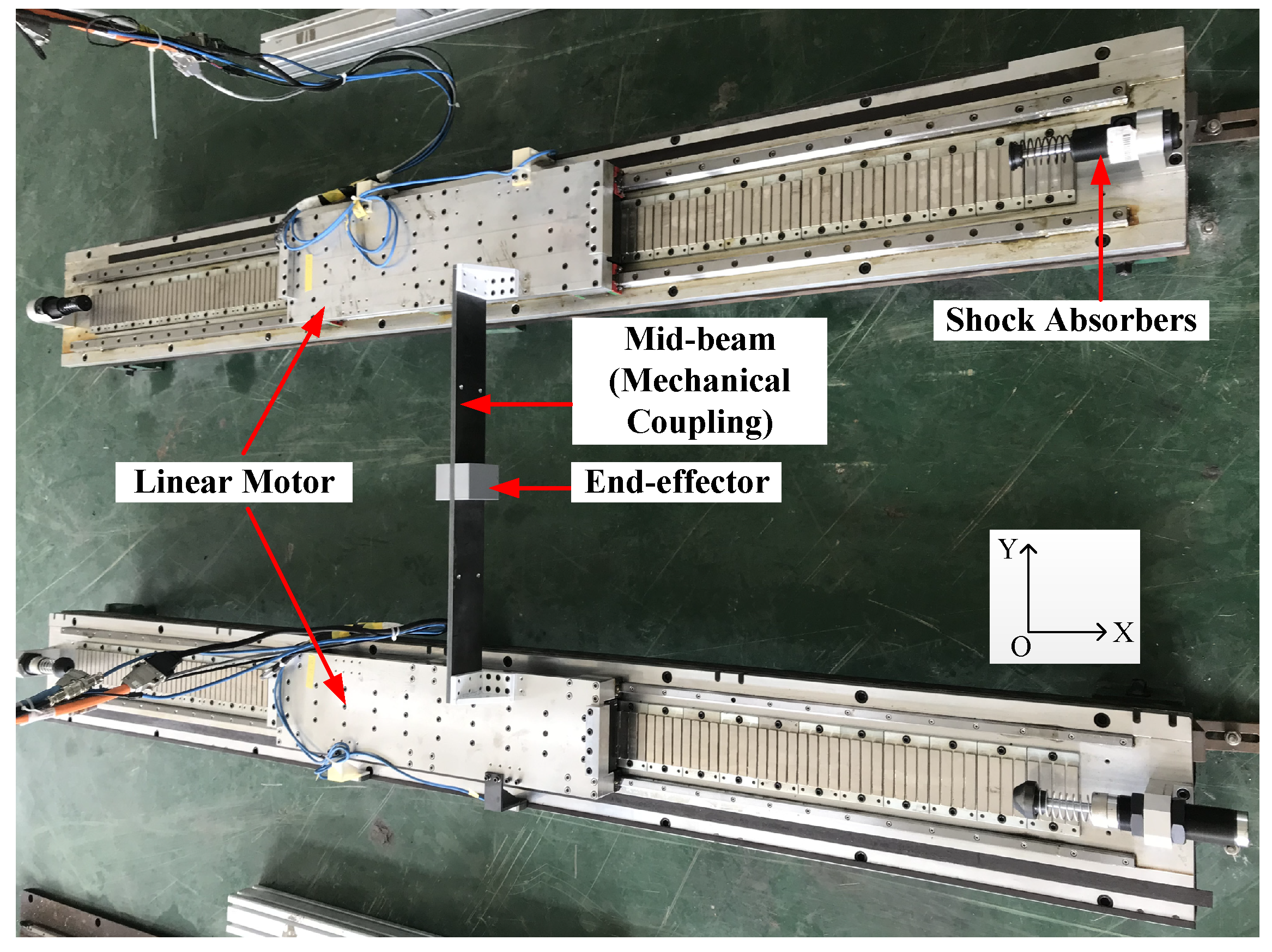
The H-type gantry stage (HGS) is widely used in electric vehicles, manufacturing automated processes, motion simulators, measuring, etc. The end-effector of HGS, such as the manipulator, specific sensor, or other equipment, moves along the mid-beam axis. Meanwhile, the mid-beam, each end of which is driven by motors, moves perpendicular to the beam axis. This configuration improves the motion stiffness, so that HGS can be applied in most engineering fields. However, the synchronization of the two motors is hard to obtain for the mechanical coupling, as shown in Figure 1.
The HGS has massive applications for machine tools. The synchronization of the two motors is achieved by improving each motor’s tracking performance. The PID controller is always adopted for each motor. This method without consideration of the mechanical coupling between the two motors is simple, but inefficient. The so-called master-slave control [1], which adopts the master motor’s output as the slave motor’s input, is also widely used. Usually, the fast motor is the slave one and is set to track the master one. However, the slave motor will accumulate the tracking error from the master one. Koren [2,3] proposed a cross-couple control (CCC) method to decrease the contour errors for manufacturing systems. This method uses a traditional controller to process the synchronous error and has been widely used in manufacturing. Similar control structures have been proposed to improve the synchronous performance of HGS. They are mostly combined with traditional PID control, e.g., PID-based on position synchronous error [4,5], PID based on velocity synchronous error [6], or the combination of the two [7,8]. These methods decrease the synchronous error, but have a poor robustness. The control parameters have to be re-tuned for different conditions. An intelligent controller is a good choice to solve this problem. Lin [9] proposed a functional link radial basis function network to adjust the control parameters in real time to improve the synchronous performance of HGS. The neural network algorithm and CCC controller were combined to enhance the robustness of each motor [10,11]. Then, they [12] designed a sliding mode controller (SMC) based on the system model and applied neural network technology on SMC to estimate the parameter uncertainty. Even though these methods can improve the synchronous performance, the neural network algorithm is time consuming and requires an additional learning process.
Currently, the nonlinear control method is widely applied in different applications, e.g., SMC [13], adaptive control (AC) [14,15,16], etc. Among these methods, AC [14,15,17] is an efficient method to process the system parameter uncertainty and can improve the system tracking performance. However, it has a poor robustness to unmodeled uncertainty or external disturbance. SMC [13] can relatively enhance the system robustness to the unmodeled uncertainty and disturbance. Yao combined the merits of AC and SMC and proposed the adaptive robust control method (ARC) [18,19,20]. The ARC adopts discontinuous projection to guarantee the boundness of uncertainty parameters in the parameter adaptive process. Combined with the robust control law, ARC achieves the global boundness of the system tracking error even with large unmodeled dynamic or external disturbance. The ARC technology has been widely used in high-precision servo systems [21,22,23,24,25]. Roy [24,25] proposed an adaptive switching-gain-based robust control (ASRC) for a class of uncertain Euler-Lagrange systems where the bound of uncertainty possesses a linear in parameters (LIP) form. It is worth noting that the ASRC no longer requires the overall uncertainty to be bounded by a constant. The uncertainty can be LIP or nonlinear in parameters (NLIP) form. Li [26] proposed an ARC method based on the linear motion equation of HGS without consideration of the mid-beam rotation, mid-beam stiffness, and end-effector movement. The synchronous performance was achieved by the so-called dynamic thrust allocation approach. He [27] then proposed a DCARCmethod based on the system model just considering the linear motion and rotation of the mid-beam. It is well-known that a precise system model will greatly improve the control performance of the model-based controller.
In this paper, an HGS driven by dual linear motors is built. The major research scope includes (1) The rigid assumed model of HGS is proposed, whose mid-beam is assumed to be a rigid-body, and mid-beam stiffness is simulated by a tensile and a torsion spring. In this multi-input-multi-output (MIMO) model, the effects of the mid-beam rotary inertia, the mid-beam stiffness, and the end-effector movement are considered. (2) Based on the proposed rigid assumed model, an adaptive robust synchronous control based on the rigid assumed model (ARSCR) is proposed. From the Lyapunov method, the proposed ARSCR can achieve the convergence of synchronous and tracking error, simultaneously.
The rest of the paper is organized as follows. In Section 2, the rigid-assumed model is proposed. In Section 3, the ARSCR is introduced, and the performance of the proposed controller is discussed. Experimental verifications are performed in Section 4 to verify the effectiveness of the proposed ARSCR, followed by a brief conclusion.
2. Nonlinear Model of HGS
2.1. Dynamic Modeling
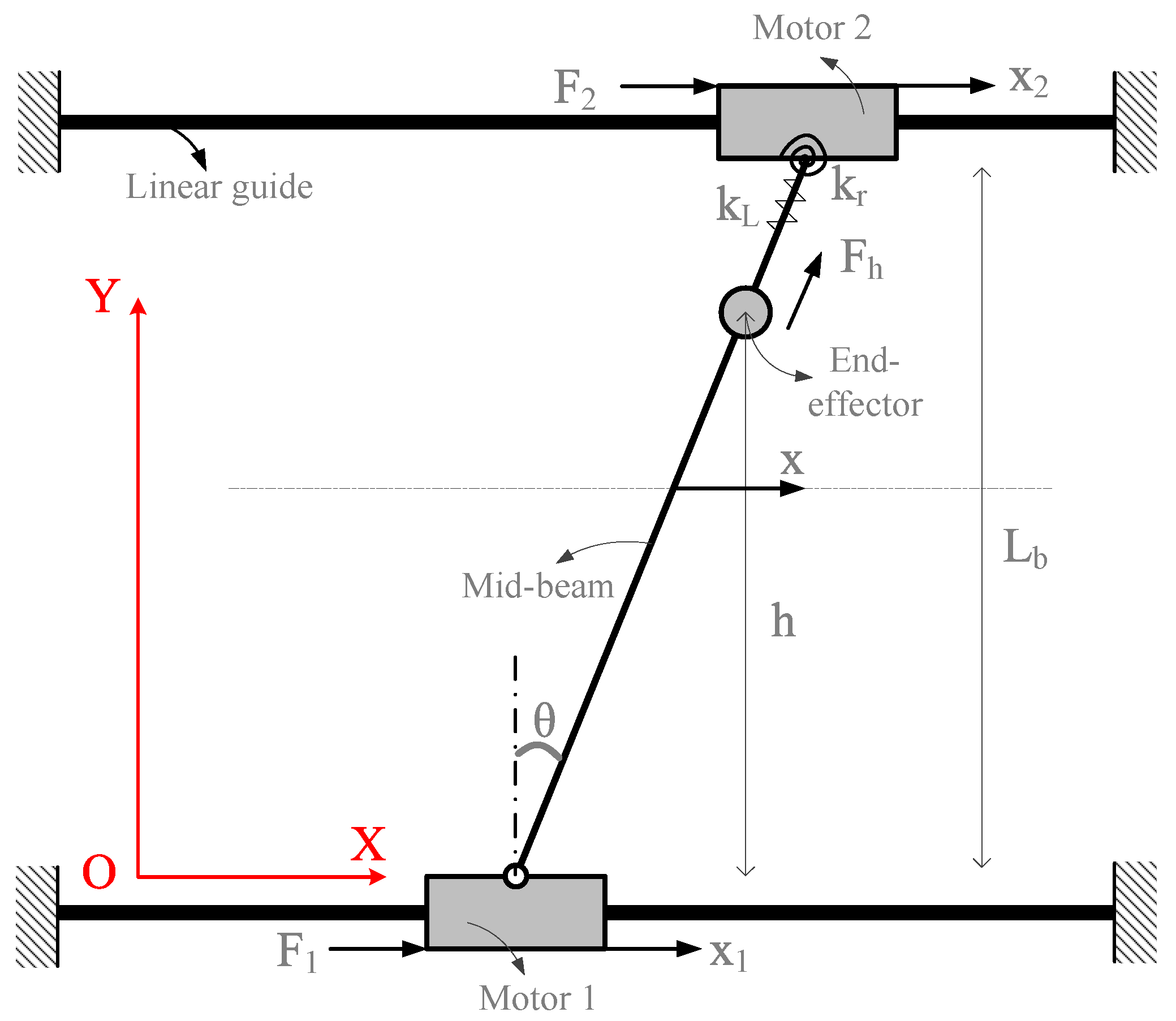
The investigated HGS is shown in Figure 2. Two linear motors move along the X direction, and the end-effector slides on the mid-beam. Two ends of the mid-beam are pined to the two linear motors respectively. To simplify the modeling process, the following assumptions are presented.
- The end-effector moves on the horizontal plane, so that the effects of gravity are ignored.
- The mid-beam is modeled as a rigid body.
- The tensile and rotational deformation of the mid-beam are modeled as a tensile spring with stiffness coefficient and a torsion spring with stiffness coefficient , respectively.
- The end-effector cannot be separated from the mid-beam.
Under these assumptions, the system kinematic energy can be obtained:
where , , , and are the kinematic energy of Linear Motor 1, Linear Motor 2, the mid-beam, and end-effector, respectively. They are expressed as:
where , , , and are the mass of Linear Motor 1, Linear Motor 2, the mid-beam, and end-effector, respectively. is the rotational inertia of the mid-beam. is the distance between the two linear motors. and are the displacement of Linear Motor 1 and Linear Motor 2, and x and are the mid-point displacement and rotary angle of the mid-beam, respectively. The dots denote the derivative with respect to time t.
These displacement variables can be converted to each other, i.e.,
where , , . Apparently, x and represent the mean and difference of two linear motors, respectively. is adopted to derive the controller, so that the tracking and synchronous error can be controlled simultaneously. The system potential energy, U, including the elastic potential energy of the tensile and torsion springs, can be expressed as:
The virtual work of all nonconservative force, , is given by:
where , , . , , and are the external force of Linear Motor 1, Linear Motor 2, and the end-effector, respectively. , , and are the virtual displacement of Linear Motor 1, Linear Motor 2, and the end-effector, respectively. and are the virtual displacement and angle of the mid-beam, respectively. The kinematic equations can be obtained from Lagrangian equations:
where is the Lagrangian function. is the generalized force obtained from . The subscripts denote the element of vector ∗. Substituting Equations (1) and (2) into Equation (4), then the system kinematic equations can be obtained:
where Equation (5) is the system force balance equation along the X direction. Equation (6) is the torque balance equation. Equation (7) is the force balance equation of the end-effector. In most practical applications, the synchronous error of the two linear motors is far less than . Therefore, , , can be established. What is more, this paper is mainly devoted to enhancing the synchronous performance of the two linear motors. Therefore, the tracking performance of the end-effector is assumed to be good enough, and Equation (7) is ignored. Based on the above assumptions, the system kinematic equations can be rewritten as:
The matrix form can be described as:
where is the mass matrix that varies with the position of the end-effector. is the inertia and Coriolis matrix introduced by the motion of the end-effector. is the stiffness matrix. They are expressed as:
The above equations show that this system is a multi-input-multi-output (MIMO) nonlinear system, and the model nonlinearity is mainly introduced by the end-effector movement and mid-beam rotary. Compensating the effects of these nonlinearities in the controller is critical to improve the system motion performance.
2.2. Friction
The effects of Coulomb friction and viscous friction are considered, i.e.,
where is the friction of linear motor i, . is the viscous friction coefficient. is the Coulomb friction coefficient. is the sign function. Rewrite Equation (11) as the vector:
where , , , and denotes the diagonal matrix. Therefore, the external force can be expressed as:
where is the control input and is the model uncertainty. Substituting Equation (12) into system kinematic Equation (10):
where is the equivalent control input and is the lumped uncertainty.
3. Nonlinear Synchronous Controller Design
3.1. Problem Formulation
The system state variables are defined as:
Then, the system kinematic Equation (13) can be rewritten as:
Define the error variable as:
where is the reference input. , . Substituting Equation (15) into Equation (14):
where:
is the vector of the uncertainty parameters and is the regressor containing the known signal. For most engineering applications, the parameter uncertainty is bounded by [26],
where , , and are the known constant vectors. “⩽” denotes the comparison among each element in vector.
3.2. Discontinuous Projection
A discontinuous projection [20,28] is introduced to guarantee the boundness of the uncertainty parameters in the adaptive process.
where , is the estimator of the uncertainty parameter . Give the following adaptive law:
where is the diagonal adaption rate matrix and is an adaption function determined during the controller design process. For any , the projection (19) guarantees the following inequalities:
where is the estimation error of uncertainty parameters. Equation (21) guarantees that the uncertainty parameters are within the defined bound in the adaptive process. Equation (22) guarantees that the discontinuous projection has no effect on the ARC design.
3.3. Controller Design
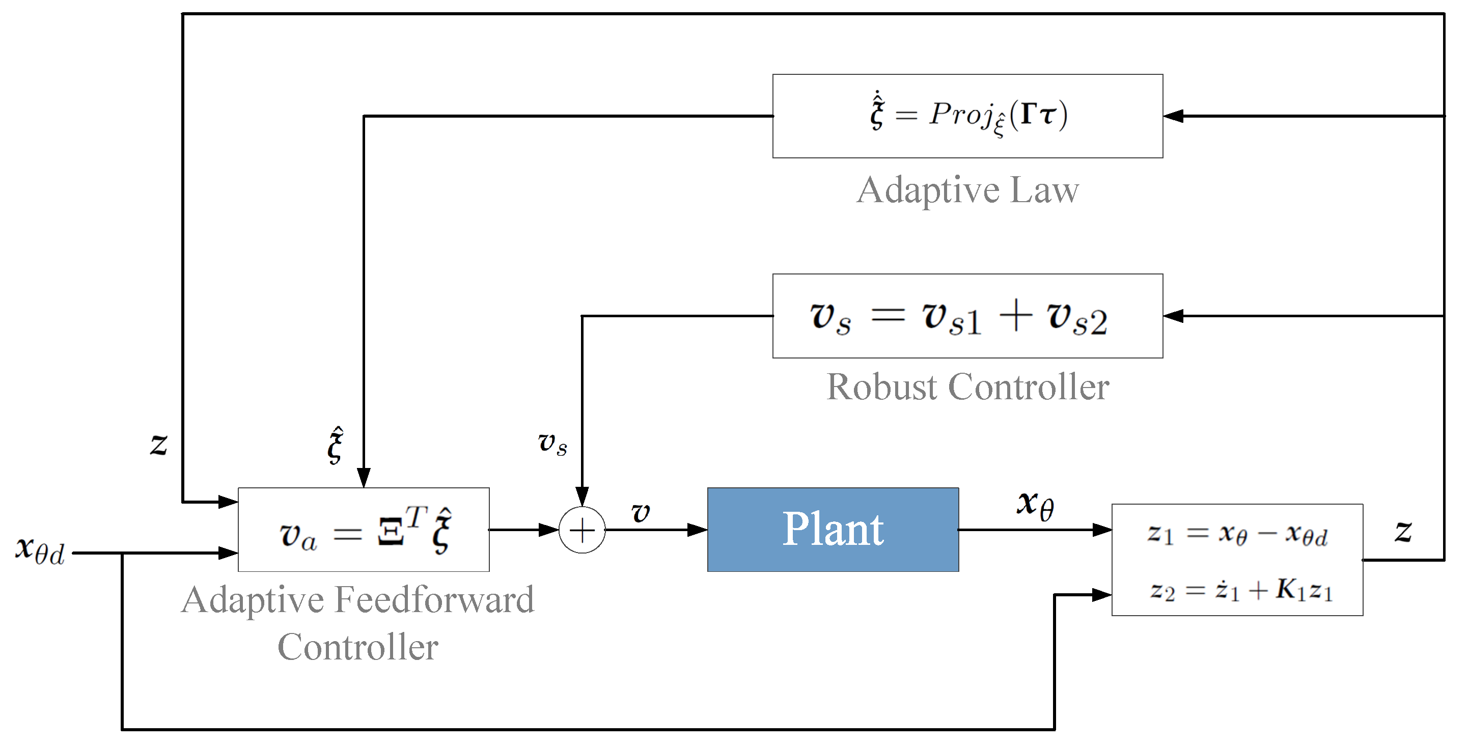
Noting the structure of Equation (16), the adaptive robust control law can be given by:
where . is the adaptive feedforward control law. Combing with the adaptive control law (20), it can efficiently compensate the parameters’ uncertainty. is the linear robust control law, and is the nonlinear robust control law. The nonlinear robust controller is designed to satisfy the following inequalities:
where , which represents the effectiveness of the model uncertainty compensating, is an arbitrary small positive number. A reasonable expression of is:
where is a positive vector. For the proof, see Appendix A. The control block diagram is shown in Figure 3.
3.4. Main Results
Define the Lyapunov function as:
where:
Apparently, and are positive matrices, so is positive. The following theorem is presented.
Theorem 1.
Give the following adaptive function:
With the adaption law (20), choosing the feedback gains matrix and large enough such that the matrix Λ defined below is positive:
then the proposed control law (23) guarantees that:
- (1)
- All system signals are bounded, and the Lyapunov function is bounded by:where , , and are the minimum and maximum eigenvalues of matrix *.
- (2)
- If there is no lumped uncertainty, i.e., , then the asymptotic convergence of system tracking and synchronous error is also achieved, i.e., , as .
Proof.
See Appendix B. ☐
From (1) in Theorem 1, the following inequality is satisfied:
The tracking performance is limited by the constant of correlating with the control gains and and mass matrix . The mass matrix is the inherent system attribute and reflects the mechanical coupling. Therefore, to achieve good tracking performance, high control gains are necessary. (1) in Theorem 1 also reveals that the proposed control law will always guarantee the boundness of the tracking and synchronous error no matter what adaption function is adopted. In other words, the uncertainty parameters are not necessarily close to their real values, but are close to the values that minimize the tracking and synchronous errors.
4. Experimental Verification
4.1. Experimental Setup
To verify the proposed synchronous controller, experiments were carried out on an HGS driven by dual linear motors shown in Figure 1. This prototype was set up in Beihang University. The amplifiers of the linear motors were S700 serials from Kollmorgen. The motor specifications are shown in Table 1. The position feedback of the two linear motors was the linear encoders with a resolution of 1 m from SIKO. Signals were collected by an NI data acquisition system. The real-time code of the control algorithm was performed in the NI RT system and realized by Labview. The sampling period was set as = 0.5 ms. The parameter values of the experimental setup are shown in Table 2. The mass was measured directly. The friction parameters were determined by the identification process. The stiffness coefficient was obtained by structural finite element analysis.
4.2. Experimental Results
Two different frequency sinusoids were adopted as the reference input: (1) low-frequency sinusoid: ; (2) high-frequency sinusoid: . They are shown in Figure 4.
Four different controller were compared to investigate the effectiveness of the proposed controller, and all controller gains were obtained by trial and error.
PD: Every linear motor adopted the traditional PD controller to realize each position feedback control. To tune the control gains, the mid-beam was disassembled, and each motor’s PD gains were tuned by trial and error. Then, the gains were fine-tuned with the mid-beam. The parameters of Linear Motor 1 were set as P controller , D controller . The parameters of Linear Motor 2 were set as P controller , D controller .
CCC: The traditional cross-couple controller was adopted to improve the system synchronous performance. The CCC control law can be expressed as:
where is the unit matrix, is the synchronous coefficient, and is the tracking error, . Each linear motor’s PD gains were first tuned the same as the previous procedures. Then, the synchronous coefficient was tuned to minimize the synchronous errors. The controller parameters were set as , , , and .
RSCR: The robust controller was adopted as a comparison. The control law is shown in Equation (23) without the adaptive process, i.e., is a constant vector. The control gains were tuned by trial and error. The controller parameters were set as and .
ARSCR: This is the proposed controller in Equation (23). The adaptive controller parameters were set as the unit matrix to tune the robust controller parameters and . Then, the adaptive controller parameters were fine-tuned to speed up the adaptive process. The robust controller parameters were set as and . The adaptive controller parameters were set as . The upper bound of the uncertainty parameters were , and the lower bound of the uncertainty parameters were . The initial values of the uncertainty parameters were .
Figure 5, Figure 6, Figure 7 and Figure 8 are the system output excited by the low-frequency sinusoid . Figure 5 is the system position tracking curve x, synchronous error , and tracking error under PD control. Figure 6 is the system position tracking curve x, synchronous error , and tracking error under CCC control. Figure 7 is the system position tracking curve x, synchronous error , and tracking error under RSCR control. Figure 8 is the system position tracking curve x, synchronous error , and tracking error under ARSCR control. The system position, synchronous error, and tracking error are defined as:
Compared with the PD controller, Figure 6 shows that the CCC controller improved the system synchronous performance efficiently, but had little effect on the tracking performance. In Figure 7, the RSCR controller not only decreased the synchronous error, but also improved the tracking performance of each motor. Compared with RSCR, the ARSCR controller achieved a better performance, as shown in Figure 8. This is because the proposed controller guaranteed the convergence of synchronous error and tracking error simultaneously. Comparing Figure 7 and Figure 8, under the adaptive feedforward control law, the errors in Figure 8 gradually became smaller and became stable after 10 s. What is more, the initial synchronous errors in Figure 8 are larger than those by PD. This is because the initial values of the uncertainty parameters were far from the real values.
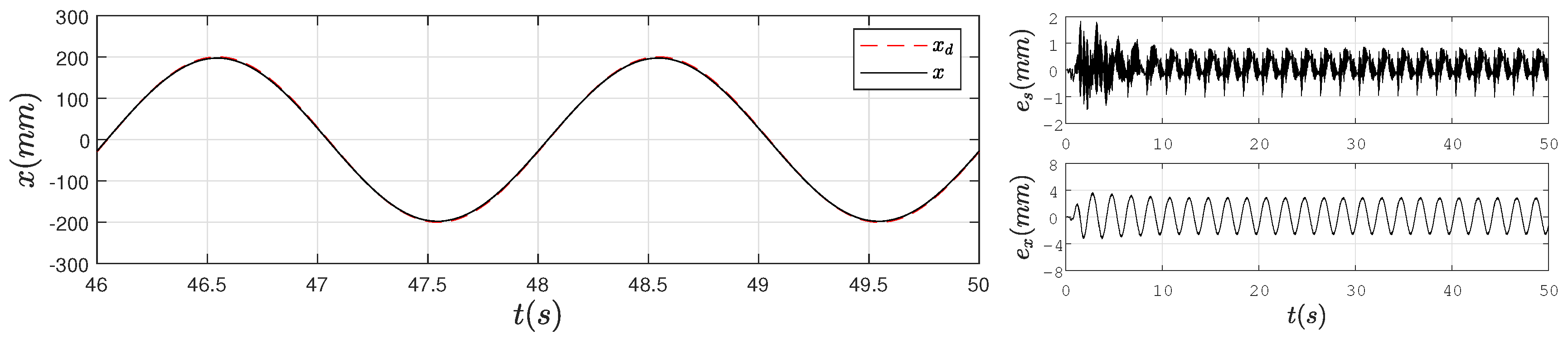
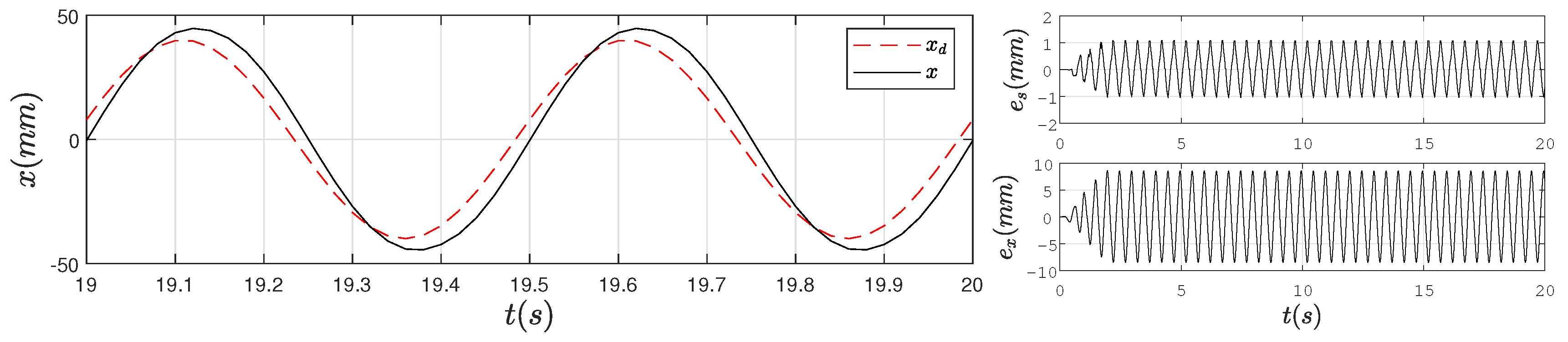
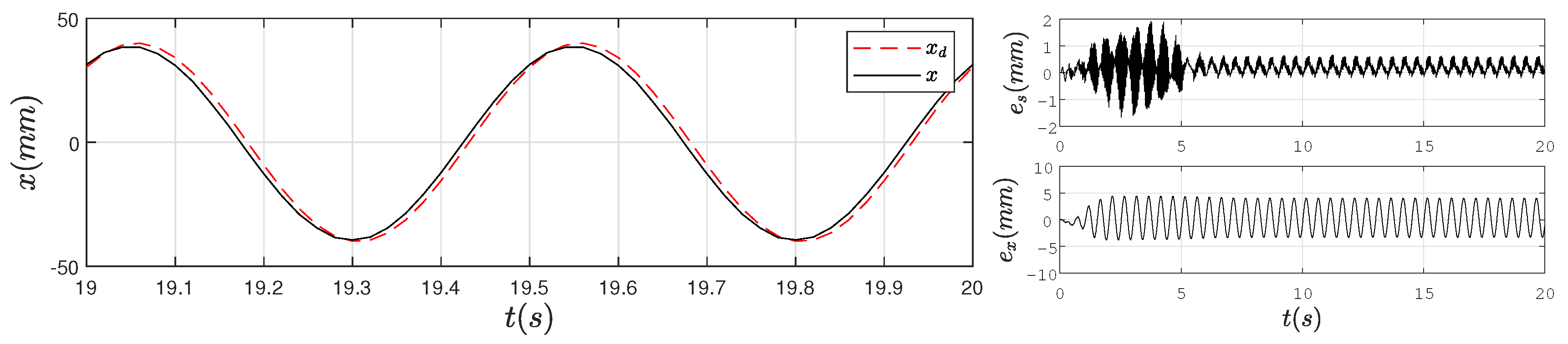
Figure 9, Figure 10 and Figure 11 are the system output excited by the high-frequency sinusoid . Figure 9 is the system position tracking curve x, synchronous error , and tracking error under PD control. Figure 10 is the system position tracking curve x, synchronous error , and tracking error under CCC control. Figure 11 is the system position tracking curve x, synchronous error , and tracking error under ARSCR control. From Figure 5 and Figure 9, the phase lag and amplitude overshoot of the system output are serious in high-frequency motion. Figure 9 and Figure 10 also show that the CCC just improves the system synchronous performance. The proposed ARSCR maintained a good performance even at a high-frequency, as shown in Figure 11. Similar to Figure 8, the errors in Figure 11 gradually become smaller and are stable after 6 s. Apparently, the higher the reference frequency, the faster the adaptation process. However, the synchronous errors chatter intensely at the beginning of Figure 11. This is because the high-frequency excitation excites the unmodeled dynamics. In high-frequency movement, the mid-beam no longer satisfies the rigid assumption, and the proposed model will be inaccurate.
5. Conclusions
In this paper, an HGS, which is widely used in electric vehicle manufacturing, driven by dual linear motors was built. A rigid assumed model of HGS, whose mid-beam was assumed to be rigid and mid-beam stiffness was simulated by a tensile and a torsion spring, was proposed. The friction was modeled as Coulomb and viscous friction. In this model, the effects of mid-beam rotary inertia, mid-beam stiffness, and end-effector movement were all taken into account. The mechanical coupling was completely described by the proposed model. Based on this model, the ARSCR method was proposed to improve both synchronous and tracking performance. From the Lyapunov method, the proposed ARSCR could achieve the convergence of synchronous error and tracking error, simultaneously. What is more, if there was no lumped uncertainty, the system tracked the desired trajectory asymptotically. Comparative experimental results showed that both the synchronous and tracking performances of ARSCR were more excellent than the traditional one, and this indicated the effectiveness of the proposed method.
Author Contributions
Conceptualization, R.C.; methodology, R.C.; software, R.C.; validation, R.C.; formal analysis, R.C.; investigation, R.C.; resources, Z.J.; data curation, R.C.; writing, original draft preparation, R.C.; writing, review and editing, L.Y.; visualization, L.Y.; supervision, L.Y., Y.S., and S.W.; project administration, Z.J.; funding acquisition, Z.J. and Y.S.
Funding
This research was funded by the National Key R&D Program of China under Grant 2017YFB1300400, the Fundamental Research on the National Defense Program of China under Grant A0420132306, the National Natural Science Foundation of China (NSFC) under grant 51875013, 51575026 and 51890882, the Fundamental Research Funds for the Central Universities, and Science and Technology on Aircraft Control Laboratory.
Acknowledgments
The authors would like to thank the support from the Collaborative Innovation Center for Advanced Aero-Engine.
Conflicts of Interest
The authors declare no conflicts of interest.
Abbreviations
The following abbreviations are used in this manuscript:
| HGS | H-type gantry stage |
| CCC | Cross-couple control |
| ARSCR | Adaptive robust synchronous control based on the rigid assumed model |
| AC | Adaptive control |
| SMC | Sliding mode control |
Appendix A
To derive the nonlinear robust control law, the inequality (27) is written as:
where and are the two columns of the regressor , respectively. To adapt the Schwarz inequality, we can rewrite the fist item on the right side of the above equation:
where . Therefore, is rewritten as:
Combining with Inequality (26):
Similarly, is rewritten as:
then:
Therefore:
Appendix B
The time derivative of the Lyapunov function (29) is expressed as:
Considering the Inequality (27):
where . Define function g:
integrating both sides of the above equation:
From the comparison principle, the following inequality is obtained:
thus, (1) in Theorem 1 is proven.
To prove (2) in Theorem 1, the following Lyapunov function is defined:
Deriving both sides of the above equation:
Thus, (2) in Theorem 1 is proven.
References
- Mochizuki, K.; Motai, T. Synchronization of Two Motion Control Axes Under Adaptive Feedforward Control. Adapt. Learn. Control 1990, 114, 196–203. [Google Scholar]
- Koren, Y. Cross-coupled biaxial computer control for manufacturing systems. J. Dyn. Syst. Meas. Control 1980, 102, 265–272. [Google Scholar] [CrossRef]
- Koren, Y.; Lo, C.C. Variable-gain cross-coupling controller for contouring. CIRP Ann. Manuf. Technol. 1991, 40, 371–374. [Google Scholar] [CrossRef]
- Byun, J.H.; Choi, M.S. A method of synchronous control system for dual parallel motion stages. Int. J. Precis. Eng. Manuf. 2012, 13, 883–889. [Google Scholar] [CrossRef]
- Giam, T.S.; Tan, K.K.; Huang, S. Precision coordinated control of multi-axis gantry stages. ISA Trans. 2007, 46, 399. [Google Scholar] [CrossRef] [PubMed]
- Yao, W.S. Modeling and synchronous control of dual mechanically coupled linear servo system. J. Dyn. Syst. Meas. Control 2015, 137, 041009. [Google Scholar] [CrossRef]
- Chen, R.; Jiao, Z.; Yan, L. Dual linear motors synchronous control for horizontal axis of far-field target motion simulators. In Proceedings of the IEEE International Conference on Aircraft Utility Systems, Beijing, China, 10–12 October 2016; pp. 810–813. [Google Scholar]
- Hsieh, M.F.; Yao, W.S.; Chiang, C.R. Modeling and synchronous control of a single-axis stage driven by dual mechanically-coupled parallel ball screws. Int. J. Adv. Manuf. Technol. 2007, 34, 933–943. [Google Scholar] [CrossRef]
- Lin, F.J.; Hsieh, H.J.; Chou, P.H.; Lin, Y.S. Digital signal processor-based cross-coupled synchronous control of dual linear motors via functional link radial basis function network. IET Control Theory Appl. 2011, 5, 552–564. [Google Scholar] [CrossRef]
- Lin, F.J.; Chou, P.H.; Chen, C.S.; Lin, Y.S. DSP-based cross-coupled synchronous control for dual linear motors via intelligent complementary sliding mode control. IEEE Trans. Ind. Electron. 2011, 59, 1061–1073. [Google Scholar] [CrossRef]
- Chou, P.H.; Chen, C.S.; Lin, F.J. DSP-based synchronous control of dual linear motors via Sugeno type fuzzy neural network compensator. J. Frankl. Inst. 2012, 349, 792–812. [Google Scholar] [CrossRef]
- Lin, F.J.; Chou, P.H.; Chen, C.S.; Lin, Y.S. Three-degree-of-freedom dynamic model-based intelligent nonsingular terminal sliding mode control for a gantry position stage. IEEE Trans. Fuzzy Syst. 2012, 20, 971–985. [Google Scholar] [CrossRef]
- He, H.; Peng, J.; Rui, X.; Hao, F. An Acceleration Slip Regulation Strategy for Four-Wheel Drive Electric Vehicles Based on Sliding Mode Control. Energies 2014, 7, 3748–3763. [Google Scholar] [CrossRef] [Green Version]
- Teo, C.S.; Tan, K.K.; Huang, S.; Lim, S.Y. Dynamic modeling and adaptive control of a multi-axial gantry stage. In Proceedings of the 2005 IEEE International Conference on Systems, Man and Cybernetics, Waikoloa, HI, USA, 12 October 2005; Volume 4, pp. 3374–3379. [Google Scholar]
- Teo, C.; Tan, K.; Lim, S.; Huang, S.; Tay, E. Dynamic modeling and adaptive control of a H-type gantry stage. Mechatronics 2007, 17, 361–367. [Google Scholar] [CrossRef]
- Tian, Y.; Xia, B.; Wang, M.; Sun, W.; Xu, Z. Comparison study on two model-based adaptive algorithms for SOC estimation of lithium-ion batteries in electric vehicles. Energies 2014, 7, 8446–8464. [Google Scholar] [CrossRef]
- Yao, J.; Jiao, Z.; Ma, D. A Practical Nonlinear Adaptive Control of Hydraulic Servomechanisms with Periodic-Like Disturbances. IEEE/ASME Trans. Mechatron. 2015, 20, 2752–2760. [Google Scholar] [CrossRef]
- Yao, B.; Tomizuka, M. Smooth Robust Adaptive Sliding Mode Control of Manipulators with Guaranteed Transient Performance. In Proceedings of the American Control Conference, Baltimore, MD, USA, 29 June–1 July 1994. [Google Scholar]
- Yao, B.; Tomizuka, M. Adaptive robust control of SISO nonlinear systems in a semi-strict feedback form. Automatica 1997, 33, 893–900. [Google Scholar] [CrossRef]
- Li, X.; Yao, B. Adaptive robust precision motion control of linear motors with negligible electrical dynamics: Theory and experiments. IEEE ASME Trans. Mechatron. 2000, 6, 444–452. [Google Scholar]
- Yao, J.; Deng, W.; Jiao, Z. RISE-Based Adaptive Control of Hydraulic Systems with Asymptotic Tracking. IEEE Trans. Autom. Sci. Eng. 2015, 14, 1524–1531. [Google Scholar] [CrossRef]
- Yao, J.; Deng, W.; Jiao, Z. Adaptive Control of Hydraulic Actuators with LuGre Model-Based Friction Compensation. IEEE Trans. Ind. Electron. 2015, 62, 6469–6477. [Google Scholar] [CrossRef]
- Sun, W.; Zhao, Z.; Gao, H. Saturated Adaptive Robust Control for Active Suspension Systems. IEEE Trans. Ind. Electron. 2013, 60, 3889–3896. [Google Scholar] [CrossRef]
- Roy, S.; Baldi, S. A Simultaneous Adaptation Law for a Class of Nonlinearly Parametrized Switched Systems. IEEE Control Syst. Lett. 2019, 3, 487–492. [Google Scholar] [CrossRef] [Green Version]
- Roy, S.; Roy, S.B.; Kar, I.N. Adaptive–robust control of euler–Lagrange systems with linearly parametrizable uncertainty bound. IEEE Trans. Control Syst. Technol. 2017, 26, 1842–1850. [Google Scholar] [CrossRef]
- Cong, L.; Yao, B.; Zhu, X.; Wang, Q. Adaptive robust synchronous control with dynamic thrust allocation of dual drive gantry stage. In Proceedings of the IEEE/ASME International Conference on Advanced Intelligent Mechatronics, Besacon, France, 8–11 July 2014. [Google Scholar]
- Li, C.; Li, C.; Chen, Z.; Yao, B. Advanced Synchronization Control of a Dual-Linear-Motor-Driven Gantry with Rotational Dynamics. IEEE Trans. Ind. Electron. 2018, 65, 7526–7535. [Google Scholar] [CrossRef]
- Sastry, S.; Bodson, M. Adaptive Control: Stability, Convergence, and Robustness; Dover Publications: Mineola, NY, USA, 1989. [Google Scholar]
Figure 1.
HGS driven by a linear motor.

Figure 2.
Structure of the investigated HGS.

Figure 3.
Control block diagram of the proposed controller.

Figure 4.
Reference input.
Figure 5.
System output under the PD controller and low-frequency excitation.
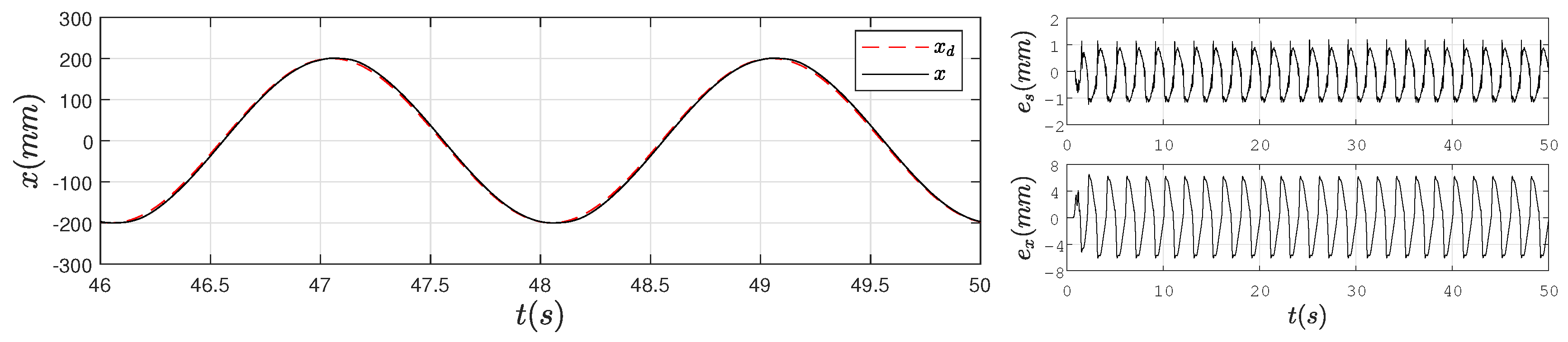
Figure 6.
System output under the CCC controller and low-frequency excitation.
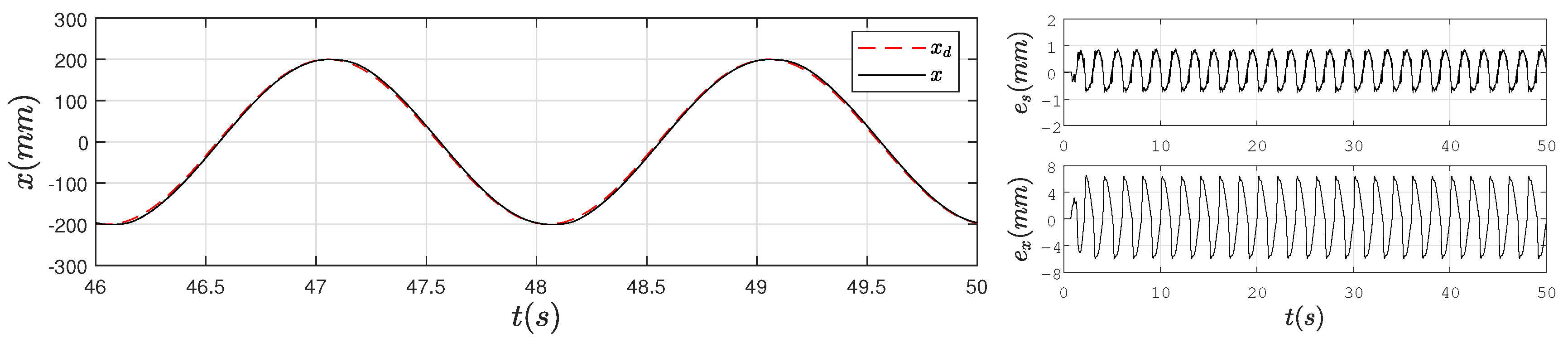
Figure 7.
System output under the RSCR controller and low-frequency excitation.
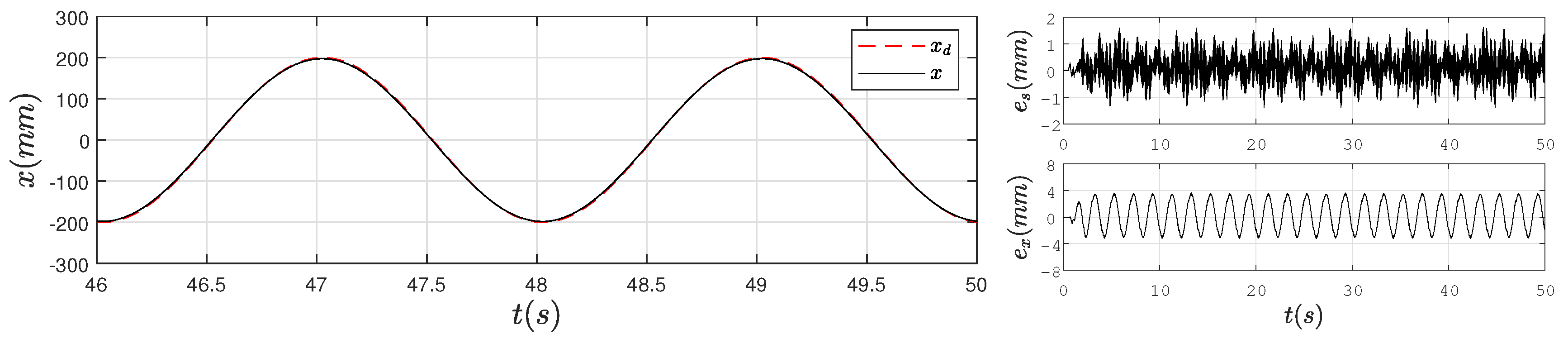
Figure 8.
System output under the ARSCR controller and low-frequency excitation.

Figure 9.
System output under the PD controller and high-frequency excitation.
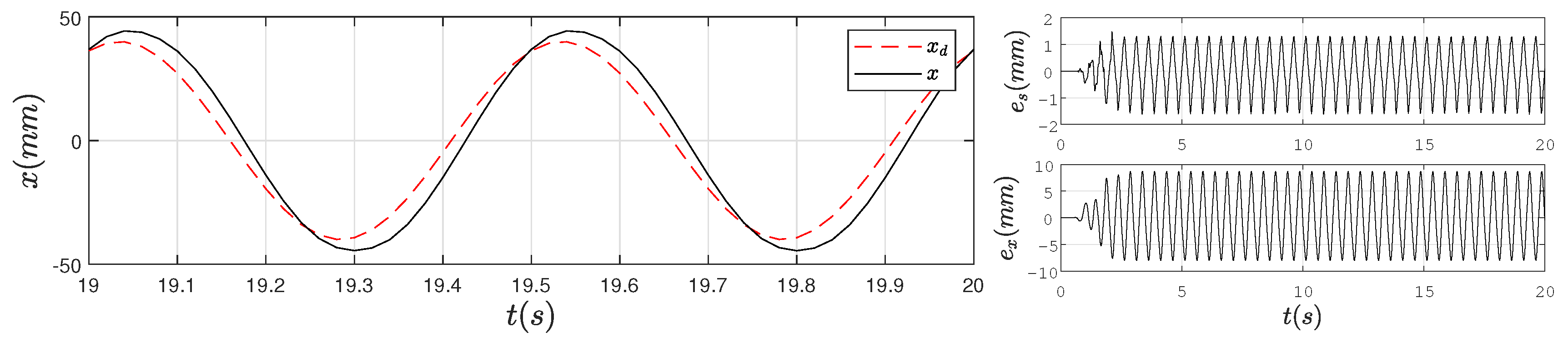
Figure 10.
System output under the CCC controller and high-frequency excitation.

Figure 11.
System output under the ARSCR controller and high-frequency excitation.

Figure 12.
Controller output under low-frequency excitation. (a) PD; (b) CCC; (c) ARSCR.
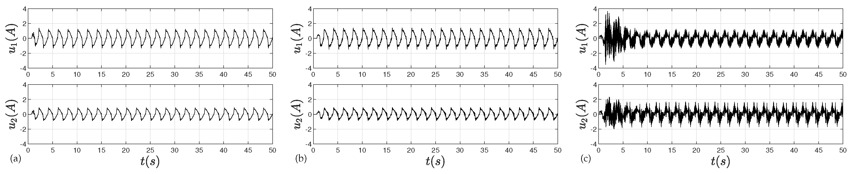
Figure 13.
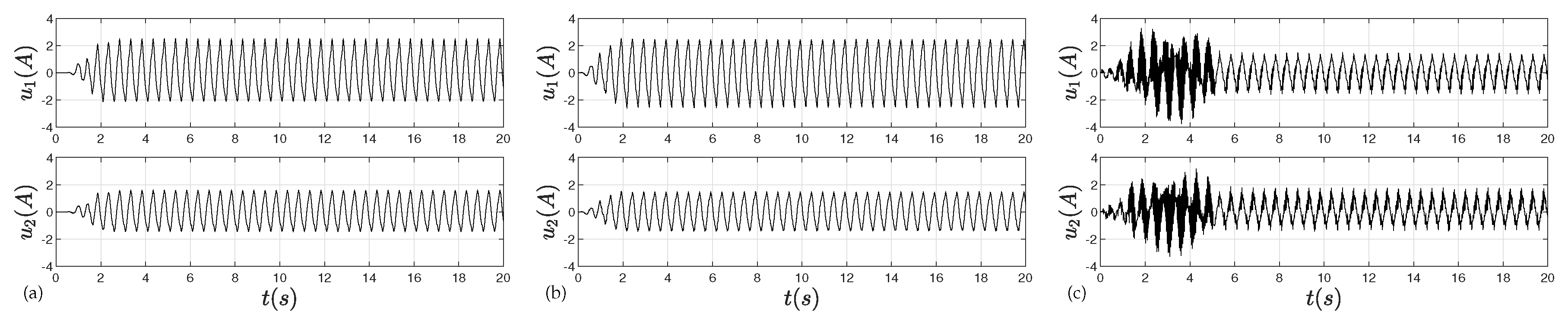
Controller output under high-frequency excitation. (a) PD; (b) CCC; (c) ARSCR.

Table 1.
Linear motor specifications.
| Model | Rated Power | Maximum Speed | Continuous Force | Continuous Current |
|---|---|---|---|---|
| Kollmorgen IC44-075 | kW | m/s | 1732 N | A |
Table 2.
Parameter values of the experimental setup.
| Symbol | Description | Value |
|---|---|---|
| mass of Linear Motor 1 | 32 kg | |
| mass of Linear Motor 2 | 28 kg | |
| mass of the mid-beam | kg | |
| mass of the end-effector | kg | |
| viscous friction coefficient of Motor 1 | N/m/s | |
| viscous friction coefficient of Motor 2 | N/m/s | |
| Coulomb friction coefficient of Motor 1 | 50 N | |
| Coulomb friction coefficient of Motor 2 | N | |
| equivalent stiffness coefficient of the mid-beam | 11,133.4 Nm/rad |
© 2019 by the authors. Licensee MDPI, Basel, Switzerland. This article is an open access article distributed under the terms and conditions of the Creative Commons Attribution (CC BY) license (http://creativecommons.org/licenses/by/4.0/).
Share and Cite
MDPI and ACS Style
Chen, R.; Jiao, Z.; Yan, L.; Shang, Y.; Wu, S. Nonlinear Synchronous Control for H-Type Gantry Stage Used in Electric Vehicles Manufacturing. Energies 2019, 12, 2305. https://doi.org/10.3390/en12122305
AMA Style
Chen R, Jiao Z, Yan L, Shang Y, Wu S. Nonlinear Synchronous Control for H-Type Gantry Stage Used in Electric Vehicles Manufacturing. Energies. 2019; 12(12):2305. https://doi.org/10.3390/en12122305
Chicago/Turabian StyleChen, Ran, Zongxia Jiao, Liang Yan, Yaoxing Shang, and Shuai Wu. 2019. "Nonlinear Synchronous Control for H-Type Gantry Stage Used in Electric Vehicles Manufacturing" Energies 12, no. 12: 2305. https://doi.org/10.3390/en12122305
Note that from the first issue of 2016, this journal uses article numbers instead of page numbers. See further details here.