Feedback Linearization and Reaching Law Based Sliding Mode Control Design for Nonlinear Hydraulic Turbine Governing System

Abstract

Hydropower as renewable energy has continually expanded at a relatively high rate in the last decade. This expansion calls for more accurate scheme design in hydraulic turbine governing system (HTGS) to ensure its high efficiency. Sliding mode control (SMC) as a robust control method which is insensitive to system uncertainties and disturbances raises interest in the application in HTGS. However, the feature of highly coupled state variables reflects the nonlinear essence of HTGS and SMC studies on the related mathematical model under certain fluctuations are not satisfied. In this regard, a novel SMC design with proportional-integral-derivative manifold is firstly applied to a nonlinear HTGS with a complex conduit system. In dealing with certain fluctuations in speed and load around the rated working condition, the proposed SMC is capable of driving the system to the desired state with smooth and light responses in aspects of the key state variables. The exponential reaching law and introduced boundary layer fasten the speed of converging time and suppress chattering. A necessary integral of sliding parameter added to manifold successfully reduces the latency caused by the anti-regulation feature of HTGS. Three operating scenarios are simulated compared with the PSO-PID method, and results imply that the proposed SMC method equips with accurate trajectory tracking ability and smooth responses. Finally, the strong robustness against system uncertainties is tested.

1. Introduction

Recently, hydropower represents an indispensable role in the power industry due to the stability, reliability and economy efficiency, compared with the developing intermittent renewable energy like solar and wind, as well as the traditional high emission coal-fired thermal power [1,2,3]. In this regard, the hydraulic turbine governing system (HTGS), as the key structure of any hydropower plant, is finely studied and designed to guarantee the operation’s safety and proper response [4]. However, the essences of HTGS are nonlinear characteristic, time-variant and a non-minimum phase system, which require efforts on precise and effective studies on practical control strategy design [5,6,7]. To overcome the obstacles in nonlinear plant controlling, considerable interests and research in the applications of HTGS regulating technique have been raised in the past several decades, such as fractional-PID control [8], fuzzy control [9], predictive control [10], adaptive control [11] and synergetic control [6,12]. However, in real time practices, there still exist problems with the specified hydraulic transients and operating conditions. In addition, the proposed control theories significantly change the structure of current HTGS which lacks applicable consideration.

Accurate modeling of HTGS matters, involving hydraulic, mechanical and electrical factors, because a precise and suitable numerical representation of the control object can better define the reliability in designing HTGS regulating techniques [4,13,14]. In the modeling conduit system, non-elastic [15] and elastic [13,16,17] models are proposed to describe the relationship between water head and flow according to conduit length. By installing a surge tank, the conduit is separated into two short parts and thus reduces the water hammer effect in the penstock [18]. Francis turbine, as one widely utilized turbine in the applications, and its proper modeling methods are a consistent topic. When considering light vibration around the operating point, Taylor series approximation equations using partial derivatives of torque and flow with respect to water head, wicket gate position, and turbine speed, are adopted [14,19]. Moreover, to ensure the regulating capability in governor design considering certain fluctuations, the partial derivatives are replaced by transfer coefficients which are varying by the states [20,21].

Though a variety of detailed mathematical models are proposed, there still exist typical discrepancies between actual plant and model due to an approximation of dynamics and variation of parameters when designing the governor [22]. In addition, existing system uncertainties and undetected noises make a difference to numerical simulations and real-time applications [23,24]. To solve these issues, the robustness of the governor has triggered intensive interest recently. Sliding mode control methodology is powerful for driving and constraining state variables to stay in the neighborhood of the designated sliding manifold, and it is successfully applied to industry and other applications such as an observer and controller combined SMC method in a solar photovoltaic-wind hybrid system [25], adaptive sub-optimal second-order SMC in micro-grids [26], global fast terminal SMC applied to water vehicles [27] and model-free based SMC to aircraft models [28]. By carefully choosing the manifold and switch function, it is capable of forcing control objects to certain states with insensitivity to model errors and rejection of disturbances. Recently, studies on SMC applied to HTGS have been carried out from every aspect: linearization based normal SMC [29], fraction-order model-based fast terminal SMC [30] and fuzzy SMC [31]. However, the studies on the performance of SMC control law facing highly coupled state variables of a nonlinear HTGS are not satisfied, as well as operating under certain fluctuations around operating points.

In this paper, a detailed nonlinear Francis turbine using six transfer coefficients is modeled to express strong coupling features of HTGS with complex conduit system. The input/output feedback linearization method is presented to construct a direct relationship between the control signal and objective state. Based on that and adopting a nonlinear servomechanism, a novel SMC method utilizing proportional-integral-derivative sliding manifold is designed by the Lyapunov method. Such method is applied to nonlinear HTGS and it shows smooth and light responses from the aspects of key state variables when facing certain fluctuations in speed and load. By adopting exponential reaching law, the system converges to a designated manifold promptly. In addition, the chattering phenomenon is eliminated by introducing a boundary layer. The anti-regulation feature of HTGS is that actual speed moves opposite to desired speed at the beginning of regulating and it causes a latency phenomenon in speed tracking. In dealing with that, a necessary integral of the sliding parameter is introduced to the manifold and thus reduces the delay in transients. Three daily met operating scenarios are simulated compared with the PSO-PID method, and the results imply that the proposed SMC method has superior trajectory tracking ability and smooth responses. Finally, the strong robustness against system uncertainties is tested.

The rest of this paper is organized as follows: Section 2 introduces the modeling process of a detailed nonlinear HTGS. In Section 3, the system is decoupled by the linearization method; the novel SMC governor design is discussed in detail and stability is proved; the PSO-PID method design as the comparison is briefly introduced. The comparative experiments and the results are discussed in Section 4. The conclusions are summarized in Section 5.

2. Mathematical Model

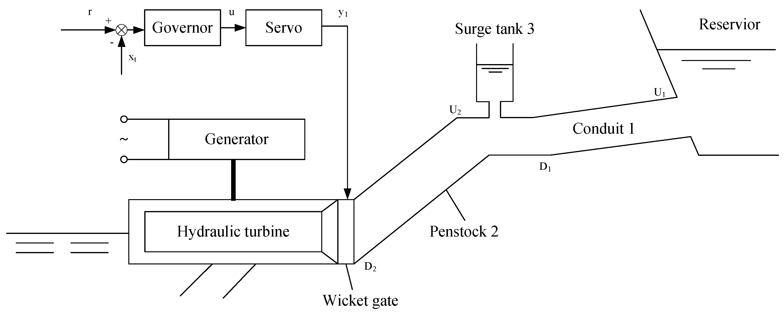
A typical hydraulic turbine governing system layout with a complex conduit system is shown in Figure 1. Water reserved in the reservoir enters into conduit 1 and passes surge tank 3 and penstock 2. Next, after passing the wicked gate which is driven by an oil hydraulic servomotor, the water flow promotes the turbine to rotate and the generator is driven as well by shaft coupling. The governor acting on a servomotor operates according to the derivation between actual and desired speed of the turbine. Therefore, HTGS is modeled including five parts: conduit system, hydraulic turbine, generator, servomotor, and governor.

2.1. Conduit System Model

The head and the flow rate equations between two cross sections of penstock are deduced from the continuity and moment equations [21], and they are defined as

$$\left[\begin{array}{c}{H}_D\left(s\right)\\ Q_D\left(s\right)\end{array}\right]=\left[\begin{array}{cc}ch\left(\gamma l\right)& -Z_{c}sh\left(\gamma l\right)\\ -\frac{sh\left(\gamma l\right)}{Z_c}& ch\left(\gamma l\right)\end{array}\right]\left[\begin{array}{c}{H}_U\left(s\right)\\ Q_U\left(s\right)\end{array}\right],$$

(1)

where $H\left(s\right)$ and $Q\left(s\right)$ are water head and flow rate in the Laplace domain, subscript U refers to the upstream section of the penstock, subscript D refers to the downstream, and l is the penstock length. In the equations, $\gamma$ and $Z_c$ are the characteristic parameters, and their expressions are defined as

$$\gamma =\sqrt{LC{s}^2+RCs}\mathrm{and}{Z}_c=\frac{\gamma }{Cs},$$

where $L=Q_r/\left(gA{H}_r\right)$, $C=\left(gA{H}_r\right)/\left(a^2{Q}_r\right)$, $R=\left(f{Q}_r^2\right)/\left(gD{A}^2{H}_r\right)$. In the expressions above, $H_r$ and $Q_r$ are water head and flow rate at the rated operating condition in the penstock, respectively. A, D and f represent cross-section area, diameter and hydraulic loss factor of the penstock, respectively.

Substituting L, C and R into $\gamma$ and $Z_c$, it is obtained:

$$\gamma \approx \frac{1}{a}s+\frac{f{Q}_r}{2aDA}\mathrm{and}{Z}_c=\frac{a{Q}_r}{gA{H}_r}+\frac{fa{Q}_r^2}{2gD{A}^2{H}_{r}s}.$$

Noting that water starting time in the penstock is $T_w=\left(Q_{r}L\right)/\left(gA{H}_r\right)$, normalized hydraulic surge impedance in the penstock $Z_p=\left(a{Q}_r\right)/\left(gA{H}_r\right)$, and elastic time of penstock $T_r=l/a$, it follows:

$$\gamma l=T_{r}s+\frac{H_f}{Z_p}$$

(2)

and

$$Z_c=Z_p+\frac{H_f}{T_{r}s},$$

(3)

where $H_f=\left(fL{V}^2/2gD\right)/H_r$ is the Darcy–Weisbach equation in the p.u. expression.

First, as conduit 1 connects to the reservoir directly, the $H_{u1}=0$, so the Equation (1) in conduit 1 is written as

$$H_{D1}=-Z_{c1}sh\left({\gamma }_1{l}_1\right)Q_{U1}\mathrm{and}{Q}_{D1}=ch\left({\gamma }_1{l}_1\right)Q_{U1}.$$

(4)

Second, the head and flow rate equation of straight-tube surge tank is expressed as

$$\frac{H_3}{Q_3}=\frac{1}{T_{j}s},$$

(5)

where $T_j$ is water starting time in the surge tank. At the conjunction of conduit 1 and penstock 2, the relationship of heads, which are nearly equal everywhere, and flow rates are obtained:

$$H_{D1}=H_3=H_{U2}\mathrm{and}{Q}_{U2}=Q_{D1}-Q_3=Q_{D1}-\left(T_{j}s\right)H_3.$$

(6)

Third, the head and flow rate equations in the penstock 2 are written as

$$\left[\begin{array}{c}{H}_{D2}\\ Q_{D2}\end{array}\right]=\left[\begin{array}{cc}ch\left({\gamma }_2{l}_2\right)& -Z_{c2}sh\left({\gamma }_2{l}_2\right)\\ -\frac{sh\left({\gamma }_2{l}_2\right)}{Z_{c2}}& ch\left({\gamma }_2{l}_2\right)\end{array}\right]\left[\begin{array}{c}{H}_{U2}\\ Q_{U2}\end{array}\right].$$

(7)

Thus, the transfer function on the downstream section of the penstock 2 is obtained:

$$G_{D2}=\frac{H_{D2}}{Q_{D2}}=\frac{ch\left({\gamma }_2{l}_2\right)H_{U2}-Z_{c2}sh\left({\gamma }_2{l}_2\right)Q_{U2}}{\frac{-sh\left({\gamma }_2{l}_2\right)}{Z_{c2}}{H}_{U2}+ch\left({\gamma }_2{l}_2\right)Q_{U2}}.$$

(8)

Furthermore, combining Equations (4), (5), (6) and (8),

$$G_{D2}=-\frac{Z_{c1}tanh\left({\gamma }_1{l}_1\right)+Z_{c2}tanh\left({\gamma }_2{l}_2\right)\left[Z_{c1}tanh\left({\gamma }_1{l}_1\right)T_{j}s+1\right]}{\frac{Z_{c1}}{Z_{c2}}tanh\left({\gamma }_1{l}_1\right)tanh\left({\gamma }_2{l}_2\right)+Z_{c1}tanh\left({\gamma }_1{l}_1\right)T_{j}s+1}$$

(9)

is obtained.

Because the surge tank divides the tunnel into two short sections, both two pipelines are modeled assuming in-compressible fluids and non-elastic conduits [18]. In this regard, express the hyperbolic tangent function, $tanh\left(\gamma l\right)$, as Taylor series and reserve one term, i.e., $\gamma l$. Noting that $Z_c\left(\gamma l\right)\approx T_{w}s+2H_f$ as $T_w=Z_p{T}_r$; $T_w\gg {H_f}^2$; thus, Equation (9) is written as

$$G_{D2}=-\frac{\left(T_{w1}s+2H_{f1}\right)+\left(T_{w2}s+2H_{f2}\right)\left[\left(T_{w1}s+2H_{f1}\right)T_{j}s+1\right]}{\frac{1}{{Z_{c2}}^2}\left(T_{w1}s+2H_{f1}\right)\left(T_{w2}s+2H_{f2}\right)+\left(T_{w1}s+2H_{f1}\right)T_{j}s+1}.$$

(10)

It denotes that Equation (10) includes hydraulic friction losses in both pipelines. Neglecting the first term of the denominator in Equation (10) because $T_{j}s$ is much larger than $T_{w2}s+2H_{f2}$, Equation (10) is simplified as

$$G_{D2}=\frac{H_{D2}}{Q_{D2}}=-\frac{\left(T_{w1}s+2H_{f1}\right)}{\left(T_{w1}s+2H_{f1}\right)T_{j}s+1}-\left(T_{w2}s+2H_{f2}\right).$$

(11)

Equation (11) in differential equation:

$$a_3+a_2\ddot{q}+a_1\dot{q}+a_{0}q=b_2\ddot{h}+b_1\dot{h}+h,$$

(12)

where

$$a_0=-2\left(H_{f1}+H_{f2}\right),a_1=-\left(T_{w1}+T_{w2}+4H_{f1}{H}_{f2}{T}_j\right),a_2=-2\left(T_{w1}{T}_j{H}_{f2}+T_{w2}{T}_j{H}_{f1}\right),$$

$$a_3=-T_{w1}{T}_{w2}{T}_j,b_1=2T_j{H}_{f1},b_2=T_{w1}{T}_j.$$

Finally, the the state-space function of Equation (12) follows:

$$\left\{\begin{array}{cc}\hfill {\dot{x}}_1& =x_2+h_{1}h,\hfill \\ \hfill {\dot{x}}_2& =x_3+h_{2}h,\hfill \\ \hfill {\dot{x}}_3& =k_1{x}_1+k_2{x}_2+k_3{x}_3+h_{3}h\hfill \end{array}\right.$$

(13)

and the output equation is

$$q=x_1+h_{0}h,$$

(14)

where

$$k_1=-\frac{2\left(H_{f1}+H_{f2}\right)}{T_{w1}{T}_{w2}{T}_j},k_2=-\frac{1}{T_{w1}{T}_j}-\frac{1}{T_{w2}{T}_j}-\frac{4H_{f1}{H}_{f2}}{T_{w1}{T}_{w2}},k_3=-\frac{2H_{f1}}{T_{w1}}-\frac{2H_{f1}}{T_{w2}},$$

$$h_0=0,h_1=-\frac{1}{T_{w2}},h_2=\frac{2H_{f2}}{T_{w2}^2},h_3=\frac{1}{T_{w2}^2{T}_j}-\frac{4H_{f2}^2}{T_{w2}^3}.$$

2.2. Hydraulic Turbine Model

The torque and flow rate equations of a Francis turbine are represented in the vicinity of a rated operating condition as a linear model by following equations with six fixed transfer coefficients [19]:

$$\left\{\begin{array}{cc}\hfill m_t& =e_x{x}_t+e_{y}y+e_{h}h,\hfill \\ \hfill q& =e_{qx}{x}_t+e_{qy}y+e_{qh}h,\hfill \end{array}\right.$$

(15)

where $m_t$, q, $x_t$, y and h represent turbine mechanical torque, turbine flow rate, turbine speed, wicket gate opening position, and turbine head, respectively. In Equation (15), constants $e_x$, $e_y$, $e_h$, $e_{qx}$, $e_{qy}$ and $e_{qh}$ are the partial derivatives of torque and flow rate with respect to $x_t$, y and h, separately [14,19].

However, in actual operation, six transfer coefficients vary with the changing of operating condition, leading to a phenomenal nonlinear characteristic. To better model this feature, six detailed nonlinear transfer expressions, coupled to state variables, are employed to Equation (15) and express them in the way of ordinary differential equations [14,18]:

$$\left\{\begin{array}{cc}\hfill {\dot{m}}_t& =e_x{\dot{x}}_t+e_y\dot{y}+e_h\dot{h},\hfill \\ \hfill \dot{h}& =\frac{\left(\dot{q}-e_{qx}{\dot{x}}_t-e_{qy}\dot{y}\right)}{e_{qh}},\hfill \end{array}\right.$$

(16)

where

$$e_y=e_{y0}\left(h+1\right),e_x=e_{x0}\sqrt{h+1},e_h=e_{h0},$$

$$e_{qy}=e_{qy0}\sqrt{h+1},e_{qx}=e_{qx0},e_{qh}=e_{qh0}/\left(x_t+1\right),$$

$e_{y0}$, $e_{x0}$, $e_{h0}$, $e_{qy0}$, $e_{qx0}$ and $e_{qh0}$ are initial transfer coefficients.

2.3. Generator Model

To clearly demonstrate the relationship between turbine speed and load, first order differential equation is adopted to model the generator and it follows [32]:

$$T_{ab}\frac{d{x}_t}{dt}+e_n{x}_t=m_t-m_{g0},$$

(17)

where $T_{ab}=T_a+T_b$, $T_a$ and $T_b$ are inertia time constants of rotating parts in turbine and load, respectively; $e_n$ is synthetic self-regulating coefficient; $m_{g0}$ is load torque.

2.4. Servomechanism Model

The servomotor is equipped as an actuator to amplify the control signal of the hydraulic turbine governor and empower the wicket gate to operate. The servomechanism is modeled by a first order differential equation:

$$\dot{y}=\frac{1}{T_y}\left(u-y\right),$$

(18)

where u is control signal of the governor.

For practical purposes, the output of the servomotor shall be limited in a certain range and, that way, the limiter is modeled with the hyperbolic tangent function:

$$y_1=tanh\left(k_{L}y\right),$$

(19)

where $y_1$ and $k_L$ are servo output and parameter of nonlinear limiter, separately. Combining Equations (18) and (19), the differential equation of servomechanism with the limiter follows:

$${\dot{y}}_1=\frac{\left(1-y_1^2\right)}{T_y}\left(k_{L}u-{tanh}^{-1}{y}_1\right).$$

(20)

Based on the above discussions, considering nonlinear limiter of servomotor, a detailed variables coupled HTGS model with complex conduit system is presented as

$$\left\{\begin{array}{cc}\hfill \dot{q}& =x_2+h_{1}h,\hfill \\ \hfill {\dot{x}}_2& =x_3+h_{2}h,\hfill \\ \hfill {\dot{x}}_3& =k_{1}q+k_2{x}_2+k_3{x}_3+h_{3}h,\hfill \\ \hfill {\dot{x}}_t& =\frac{\left[\left(e_x-e_n\right)x_t+e_y{y}_1+e_{h}h-m_{g0}\right]}{T_{ab}},\hfill \\ \hfill \dot{h}& =\frac{x_2+h_{1}h-\frac{e_{qx}}{T_{ab}}\left[\left(e_x-e_n\right)x_t+e_y{y}_1+e_{h}h-m_{g0}\right]-\frac{e_{qy}}{T_y}\left(1-y_1^2\right)\left(k_{L}u-{tanh}^{-1}{y}_1\right)}{e_{qh}},\hfill \\ \hfill {\dot{y}}_1& =\frac{1-y_1^2}{T_y}\left(k_{L}u-{tanh}^{-1}{y}_1\right).\hfill \end{array}\right.$$

(21)

When considering system uncertainties, simply add uncertainty terms $d_1$, $d_2$, $d_3$, $d_4$, $d_5$ and $d_6$ to the end of the above equations separately. Thus, the nonlinear HTGS considering system uncertainties are given in Equation (21), in which the control signal u and objective state variable $x_t$ are not connected directly. In this regard, the direct relationship between u and $x_t$ will be constructed and the SMC governor is accordingly designed in the next section.

3. Governor Design

The proportional-integral-derivative control law is applied in HTGS universally. A PID governor drives turbine speed $x_t$ to track the desired rated speed $r_{x_t}$ by accepting the derivation of two variables, and then outputting control signals to the servomotor, which acts on the wicket gate. In this way, the PID governor is typically a single-input and single-output control system. For practical engineering applications, it is applicable to follow the same input/output design of PID control law without significantly changing the structure of governor. However, some studies apply a set of SMC governor outputs on each equation of HTGS model, which are more like an observer and not suitable for the current applications. Moreover, linearization and reaching law based SMC shows superior ability facing both fluctuations in speed and load. At the meantime, the system state variables responses are light and smooth and quickly converge to the desired point.

In this section, a sliding mode control law based on input/output feedback linearization is designed with several variables as input for computing to comply with the above criterion.

3.1. Input/Output Feedback Linearization on HTGS

In the mathematical model (21), governor output u is connected with turbine speed $x_t$ indirectly, which leads to difficulty in designing control law. Therefore, in order to obtain the direct connection between two variables, we differentiate ${\dot{x}}_t$ as below via I/O feedback linearization method [33]:

$$\begin{array}{ll}{\dot{x}}_t\hfill & =\frac{\left[\left(e_x-e_n\right)x_t+e_y{y}_1+e_{h}h-m_{g0}\right]}{T_{ab}}+d_4,\hfill \\ {\ddot{x}}_t\hfill & =\frac{1}{T_{ab}}\left\{\frac{\left(e_x-e_n\right)}{T_{ab}}\left[\left(e_x-e_n\right)x_t+e_y{y}_1+e_{h}h\right]-e_y\frac{\left(1-y_1^2\right)}{T_y}{tanh}^{-1}{y}_1\right.\hfill \\ & \left.+\frac{e_h}{e_{qh}}\left[x_2+h_{1}h-\frac{e_{qx}}{T_{ab}}\left(\left(e_x-e_n\right)x_t+e_y{y}_1+e_{h}h\right)+\frac{e_{qy}}{T_y}\left(1-y_1^2\right){tanh}^{-1}{y}_1\right]\right\}\hfill \\ & +\frac{1}{T_{ab}}\left[\frac{e_y}{T_y}-\frac{e_{qy}}{e_{qh}}\frac{e_h}{T_y}\right]\left(1-y_1^2\right)k_{L}u\hfill \\ & +\frac{1}{T_{ab}}\left[\frac{e_{qx}}{e_{qh}}\frac{e_h}{T_{ab}}-\frac{\left(e_x-e_n\right)}{T_{ab}}\right]m_{g0}-\frac{{\dot{m}}_{g0}}{T_{ab}}\hfill \\ & +\frac{1}{T_{ab}}\left[e_h{d}_5+\left(e_x-e_n\right)d_4+e_y{d}_6\right]+{\dot{d}}_4\hfill \end{array}$$

and it is simplified as

$${\ddot{x}}_t=A+Bu+M+D.$$

(22)

In Equation (22), function A, B, M and D are defined as:

$$\begin{array}{ll}A& =\frac{1}{T_{ab}}\left\{\frac{\left(e_x-e_n\right)}{T_{ab}}\left[\left(e_x-e_n\right)x_t+e_y{y}_1+e_{h}h\right]-e_y\frac{\left(1-y_1^2\right)}{T_y}{tanh}^{-1}{y}_1\right.\hfill \\ & \left.+\frac{e_h}{e_{qh}}\left[x_2+h_{1}h-\frac{e_{qx}}{T_{ab}}\left(\left(e_x-e_n\right)x_t+e_y{y}_1+e_{h}h\right)+\frac{e_{qy}}{T_y}\left(1-y_1^2\right){tanh}^{-1}{y}_1\right]\right\},\hfill \\ \hfill B& =\frac{1}{T_{ab}}\left[\frac{e_y}{T_y}-\frac{e_{qy}}{e_{qh}}\frac{e_h}{T_y}\right]\left(1-y_1^2\right)k_L,\hfill \\ \hfill M& =\frac{1}{T_{ab}}\left[\frac{e_{qx}}{e_{qh}}\frac{e_h}{T_{ab}}-\frac{\left(e_x-e_n\right)}{T_{ab}}\right]m_{g0}-\frac{{\dot{m}}_{g0}}{T_{ab}},\hfill \\ \hfill D& =\frac{1}{T_{ab}}\left[e_h{d}_5+\left(e_x-e_n\right)d_4+e_y{d}_6\right]+{\dot{d}}_4.\hfill \end{array}$$

Consequently, the ${\ddot{x}}_t$ consists of four terms: A, M, $Bu$ and D. A implies that turbine speed $x_t$ is influenced by other state variables, in other way, variables are coupled to others. In addition, M reflects that the load combining with its derivative also influences turbine speed. D indicates that related system uncertainties combining with their derivatives affect the $x_t$ intrinsically. In this way, the control term $Bu$ designed in the next subsection aims to get equivalent AM and D to keep $x_t$ at a rated speed. Thus, the direct relationship between turbine speed $x_t$ and governor signal u is established. In addition, an SMC control law acted on $x_t$ is easy to design next.

3.2. SMC Control Law Design

Because of the nonlinear natures of HTGS, there are tremendous obstacles in controlling the turbine to the desired state. The anti-regulation feature mentioned above causes a significant latency in speed tracking. To reduce such delay, a necessary integral of sliding parameter is introduced to the manifold and thus a PID sliding manifold is selected. To fasten the sliding variable s approaching manifold when s is much larger, which is useful when facing large fluctuation, exponential reaching law is adopted [34]. Thus, the SMC governor is qualified in overcoming the complexity of the nonlinear model.

In order to drive $x_t$ to track the desired trajectory, set the speed error as $e=r_{x_t}-x_t$, and then, to reduce the error when facing strong coupling features of state variables, the PID sliding manifold is selected as:

$$s={\lambda }_{p}e+{\lambda }_i\int e+{\lambda }_d\dot{e},$$

(23)

where parameters ${\lambda }_p$ and ${\lambda }_d$ must satisfy Hurwitz condition and ${\lambda }_i\ge 0$. Next, differentiate s and it follows:

$$\dot{s}={\lambda }_p\dot{e}+{\lambda }_{i}e+{\lambda }_d\ddot{e}={\lambda }_p\dot{e}+{\lambda }_{i}e+{\lambda }_d{\ddot{r}}_{x_t}-{\lambda }_d{\ddot{x}}_t.$$

Substituting Equation (22) in the above equation, it is given that

$$\dot{s}={\lambda }_p\dot{e}+{\lambda }_{i}e+{\lambda }_d{\ddot{r}}_{x_t}-{\lambda }_d\left(A+Bu+M+D\right).$$

(24)

Set control signal as:

$$u=\frac{v}{B},$$

(25)

where v is the auxiliary controller. Then, based on exponential reaching law, by adding the exponential term $-ks$, $\dot{s}$ is given below:

$$\dot{s}={\lambda }_p\dot{e}+{\lambda }_{i}e+{\lambda }_d{\ddot{r}}_{x_t}-{\lambda }_d\left(A+Bu+M\right)={\lambda }_d\left(-\eta sign\left(s\right)-ks\right).$$

It denotes that, when designing an auxiliary controller, D is not taken into consideration because it is the uncertainties of the system, which cannot be detected but will be eliminated by tuning the gain of boundary layer $\eta$ discussed below. Thus, v follows

$$v={\ddot{r}}_{x_t}-A-M+\frac{1}{{\lambda }_d}\left({\lambda }_p\dot{e}+{\lambda }_{i}e\right)+\eta sign\left(s\right)+ks,\eta >0,k>0.$$

(26)

$\eta$ is a positive constant and satisfies $\eta >\left|D_r\right|$, in which $D_r$ is the upper boundary of system uncertainties D.

In the following section, the stability analysis is given.

3.3. Stability Analysis

Consider the nonlinear model of HTGS with complex conduit system and system uncertainties, as shown in Equation (21). The proposed SMC control law, if the control signal complies with Equation (25), guarantees the stability of the mentioned system and drives speed error $e=r_{x_t}-x_t$ to converge to zero asymptotically. The proof is given below.

Proof. 

Select the Lyapunov function as:

$$V=\frac{1}{2}{s}^2,$$

whose derivative is

$$\dot{V}=s\dot{s}=s\left[{\lambda }_p\dot{e}+{\lambda }_{i}e+{\lambda }_d{\ddot{r}}_{x_t}-{\lambda }_d\left(A+Bu+M+D\right)\right].$$

Combining Equation (25) and Equation (26),

$$\dot{V}=-{\lambda }_{d}s\left[\eta sign\left(s\right)+D+ks\right]=-{\lambda }_d\left[\eta \left|s\right|+Ds+k{s}^2\right].$$

Thus,

$$\dot{V}=\left\{\begin{array}{c}-{\lambda }_d\left[\left(\eta +D\right)s+k{s}^2\right],s\ge 0,\hfill \\ -{\lambda }_d\left[\left(D-\eta \right)s+k{s}^2\right],s<0.\hfill \end{array}\right.$$

(27)

According to Equation (27), $\dot{V}\le 0$ because, as mentioned above, the gain $\eta$ is set larger than the upper boundary of D. In this way, the attractiveness of PID sliding manifold is guaranteed.

Thus, according to Lyapunov stability theorem, the system is asymptotically stable, and the speed error will converge to zero within a finite time, which implies that the SMC governor is capable of driving the system to any point or orbit. ☐

3.4. Chattering Phenomenon Elimination

One marked imperfection of SMC control law is that, when a state variable reaches sliding manifold, it moves around a manifold frequently rather than sliding along with it. The reason is that SMC control law adopts a discontinuous sign function, which makes the sliding parameter become equipped with inertia even when it is located right on the manifold [22].

In order to restrain the chattering phenomenon, the saturated function $sat\left(s\right)$ within the boundary is introduced instead of a sign function in Equation (26), and $sat\left(s\right)$ is defined as

$$sat\left(s\right)=\left\{\begin{array}{c}sign\left(s\right),abs\left(s\right)\ge \delta ,\hfill \\ k_{p}s,abs\left(s\right)<\Delta ,k_p=\frac{1}{\delta },\hfill \end{array}\right.$$

(28)

in which $\delta$ is the thickness of the boundary layer. When s is located outside the boundary layer, the switch control using sign function is adopted and, when s is inside the boundary layer, a smooth control is adopted rather than switching vigorously. Therefore, the chattering phenomenon is eliminated markedly.

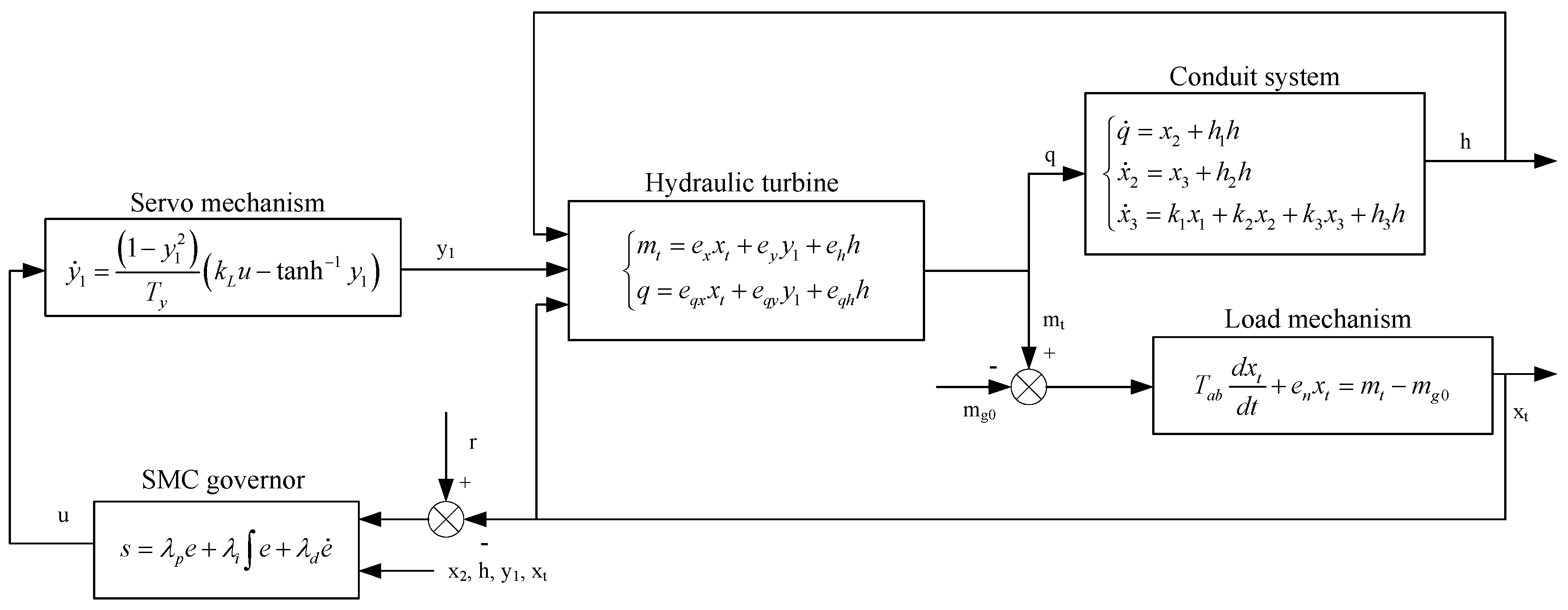
Thus, a novel SMC governed HTGS system is presented and shown in Figure 2.

3.5. PSO-PID Governor Design as Comparison

Currently, traditional PID control law is widely applied in HTGS because of its reliability. Its equation follows:

$$u=k_p\left(r_{x_t}-x_t\right)+k_i\int \left(r_{x_t}-x_t\right)+k_{d}d\left(r_{x_t}-x_t\right).$$

(29)

In addition, for better performance of the controller, three important parameters, $k_p$, $k_i$ and $k_d$, require a suitable method to tune with according to various operating conditions. The particle swarm optimization (PSO) algorithm, one of many evolution algorithms aiming at searching for a suitable solution from populational sets [35], and its variants are populated in PID parameters tuning for HTGS. Based on former studies [36,37], a modified weight-varying PSO algorithm is adopted as:

$$v_{ik}\left(t+1\right)=\omega v_{ik}\left(t\right)+c_{1}r\left(P_{ik}\left(t\right)-X_{ik}\left(t\right)\right)+c_{2}r\left(P_{gk}\left(t\right)-X_{ik}\left(t\right)\right),$$

(30)

where weight $\omega$ is varying by iterations, $\omega =N_{iter}\left({\omega }_{Max}-{\omega }_{Min}\right)/N$, in which $N_{iter}$ and N are current iteration and total iteration times, respectively; ${\omega }_{Max}$ and ${\omega }_{Min}$ are initial maximum and minimum weights.

However, due to the complexity of nonlinear servomotor and coupled variables hydraulic turbine, it shows tremendous difficulties in optimizing parameters. Particularly, the optimizing process easily returns complex numbers, which is meaningless in practice. Thus, during optimizing, it introduces an elimination mechanism, which means, once the optimization process using certain PID parameters returns a set of complex results, these three parameters will be discarded to guarantee the process to continue.

In addition, a reliable criterion in the HTGS parameter tuning field, the minimization of the integral of time-weighted absolute error (ITAE) [38], is adopted as the fitness function of selected PSO optimizing process and its expression is:

$$J_{ITAE}={\int }_0^{T}t\left|e\left(t\right)\right|dt,$$

(31)

where T is simulation time.

The optimization process starts at initializing the swarm in which each particle includes $k_p$, $k_i$ and $k_d$ as its position. Then, evaluate the particles’ fitness by the above ITAE criterion. According to the fitness results, update individual performance and select the global swarm best performance. The next step is to modify the particles’ velocities and update particles’ positions until the iteration ends. The final best position is the optimization result of PSO-PID control parameters. PSO with the ITAE criterion is also used to help select the parameters of the PID sliding manifold by replacing position $k_p$, $k_i$ and $k_d$ with ${\lambda }_p$, ${\lambda }_i$, ${\lambda }_d$.

The effectiveness of the proposed SMC method compared to PSO-PID control will be validated and the SMC control parameters calculating standards is given in the next section.

4. Results and Discussion

In this section, the validity and effectiveness analysis of SMC governor designed in Section 3 operating on the nonlinear HTGS model (21) will be discussed for three scenarios: target turbine speed stabilization is simulated to validate the smooth and light responses facing changes in speed; periodic turbine speed trajectory tracking is conducted to validate that the latency is fully reduced by an integral term in the sliding manifold; and load disturbance response testing is conducted to testify the efficiency of SMC in power output control, as well as strong robustness simulation against system uncertainties. The aforementioned PID controller based on the PSO algorithm with the elimination mechanism and ITAE criterion, which is discussed above, is adopted as a comparison to illustrate the strength of the SMC controller. While the parameters of proposed SMC method consist of three parts: the gain $\eta$ of boundary layer, coefficients k of reaching law term and selection of sliding manifold parameters ${\lambda }_p$, ${\lambda }_i$, ${\lambda }_d$. $\eta$ is set larger than the upper boundary of D as mentioned to suppress the system disturbances. In addition, in order to accelerate converging time facing large fluctuations such as periodic speed tracking and large load shedding, the k is given larger. While the selection of sliding manifold is to guarantee the speed error e converge to zero, and PSO also helps to select the combination of three parameters. All the simulations are started at rated working condition, which indicates that the initial relative derivation values of q, $x_2$, $x_3$, $x_t$, h and $y_1$ are zero. To be noticed, when $y_1$ is set as zero which means the setting relative derivation value of wicket gate has the opposite range of proposed servomechanism, thus the computed control signal u needs to multiply by an adjusting coefficient $-1$. All the simulations are conducted utilizing a Runge–Kutta method with a variable time step under the MATLAB/Simulink environment. The system parameters are listed in Appendix A.

4.1. Target Turbine Speed Stabilization

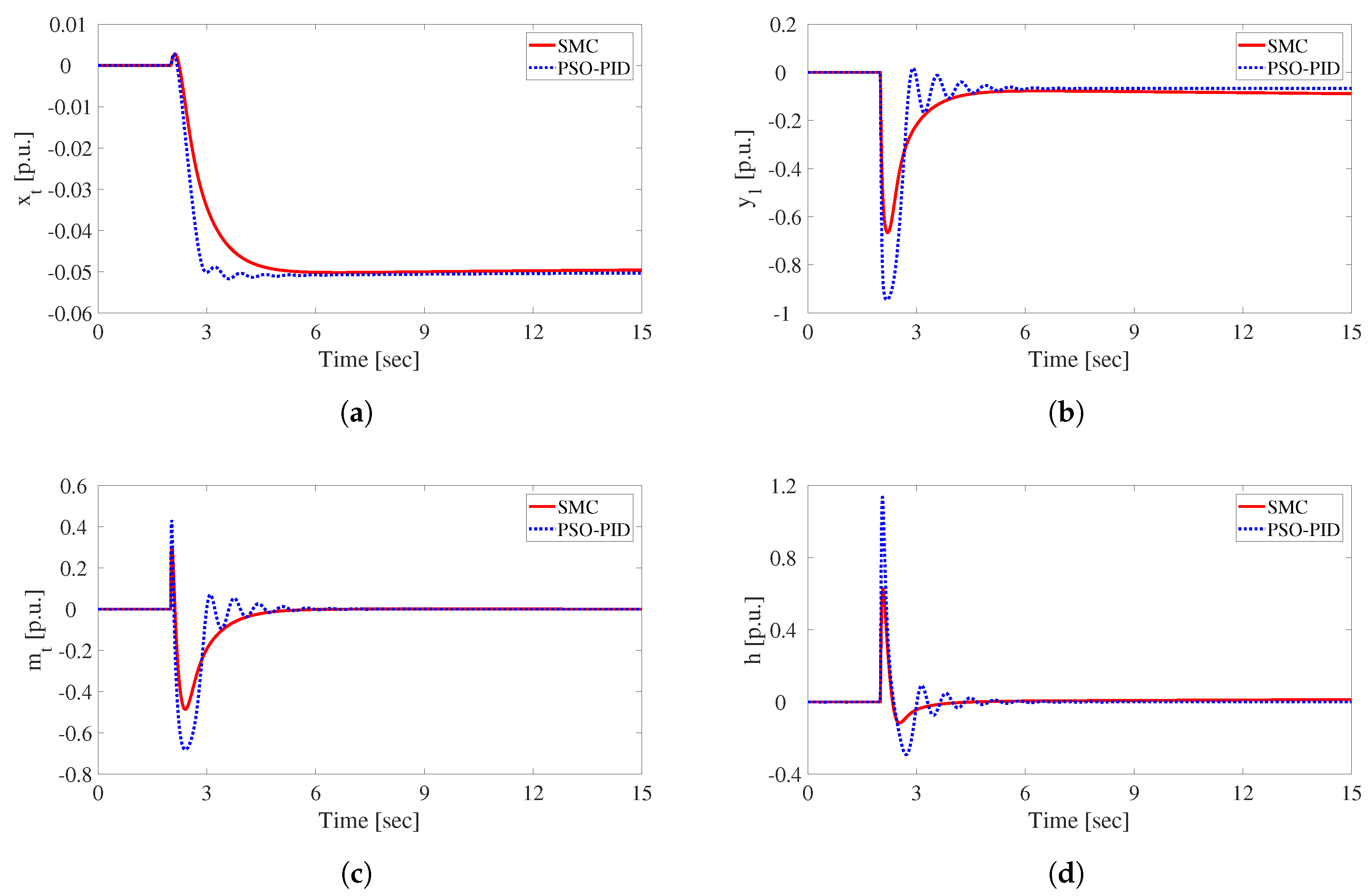
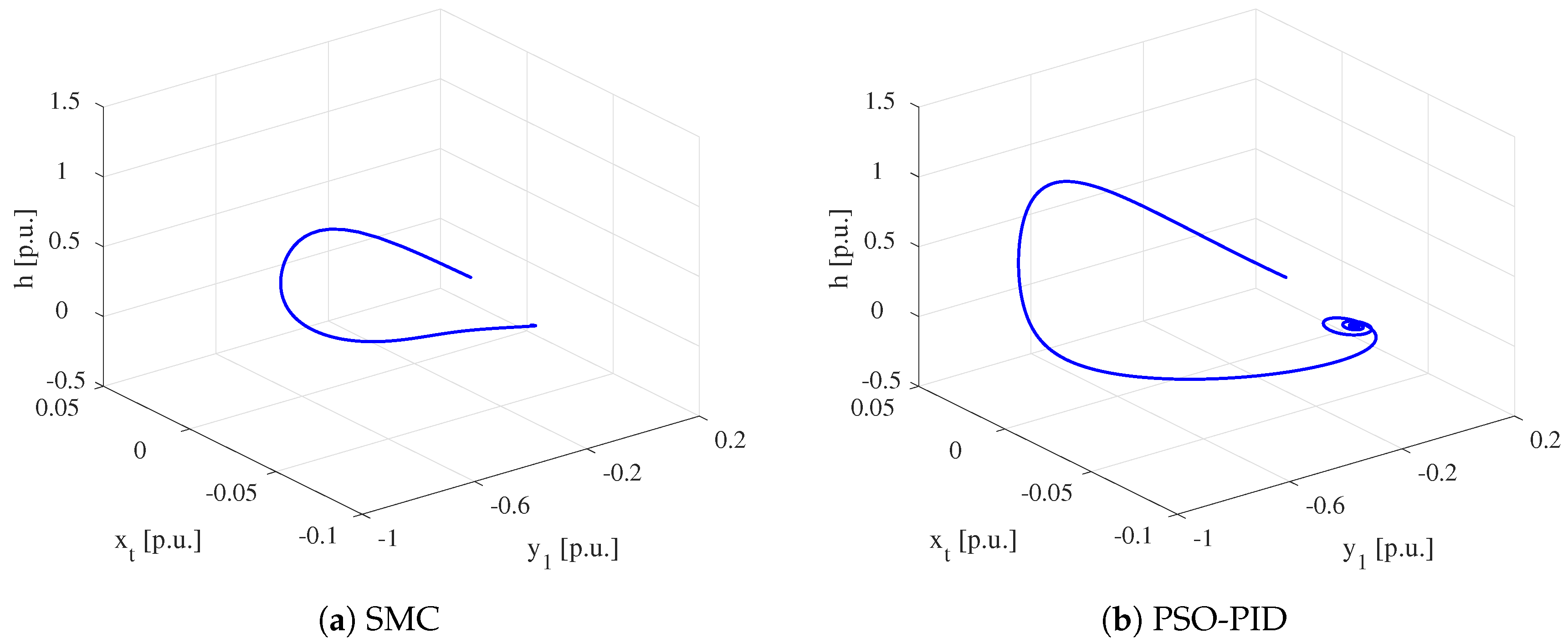
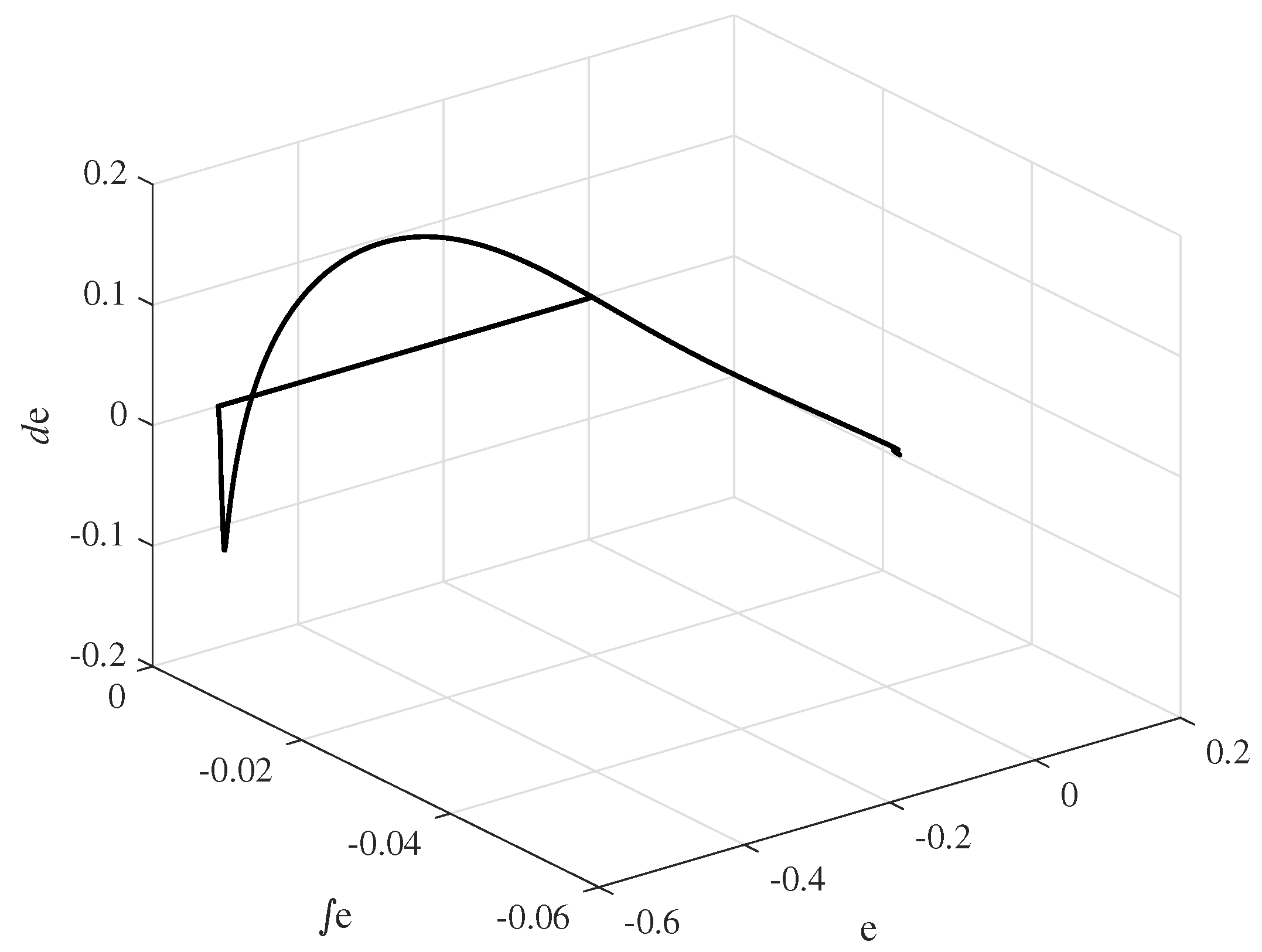
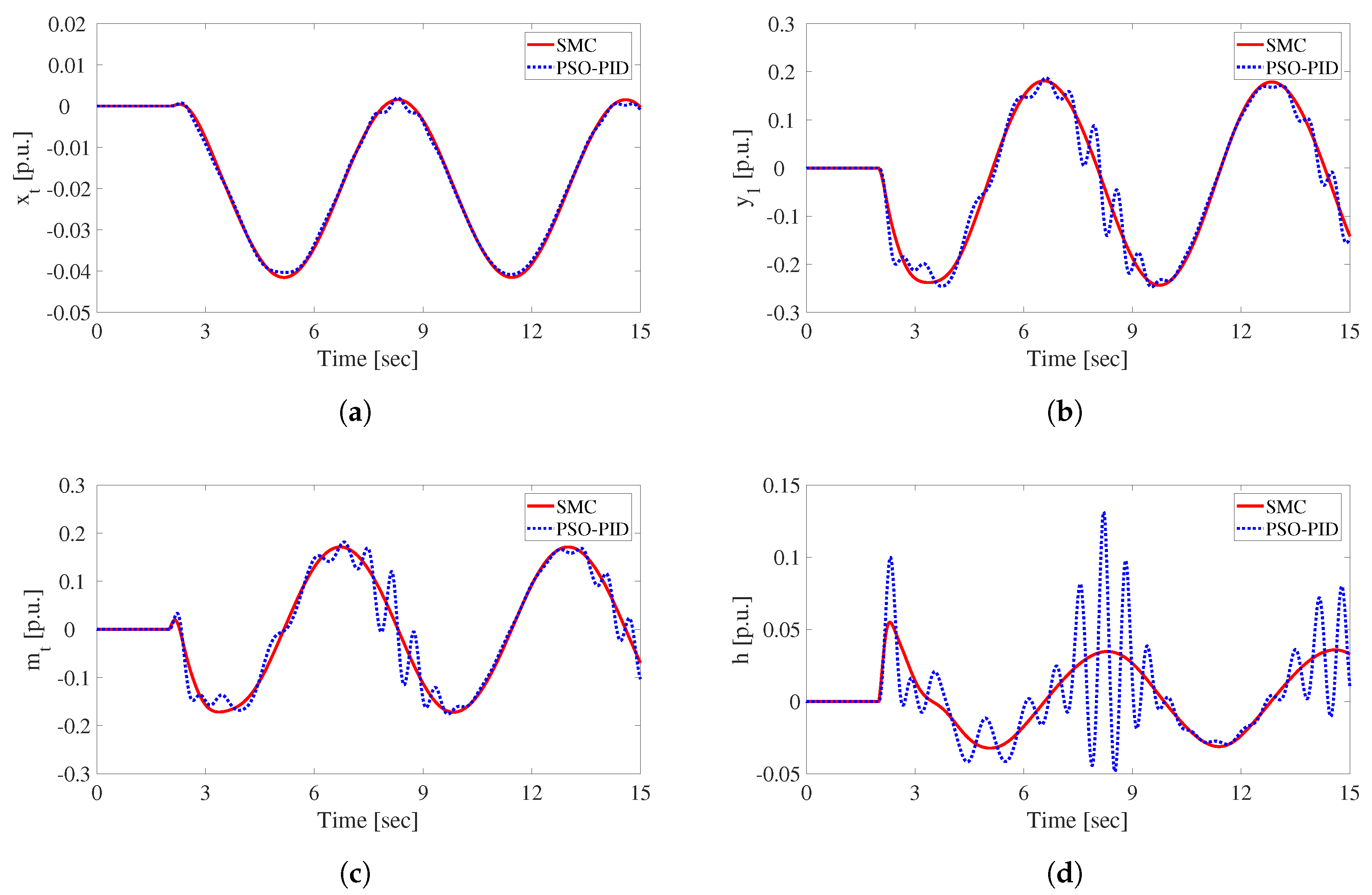
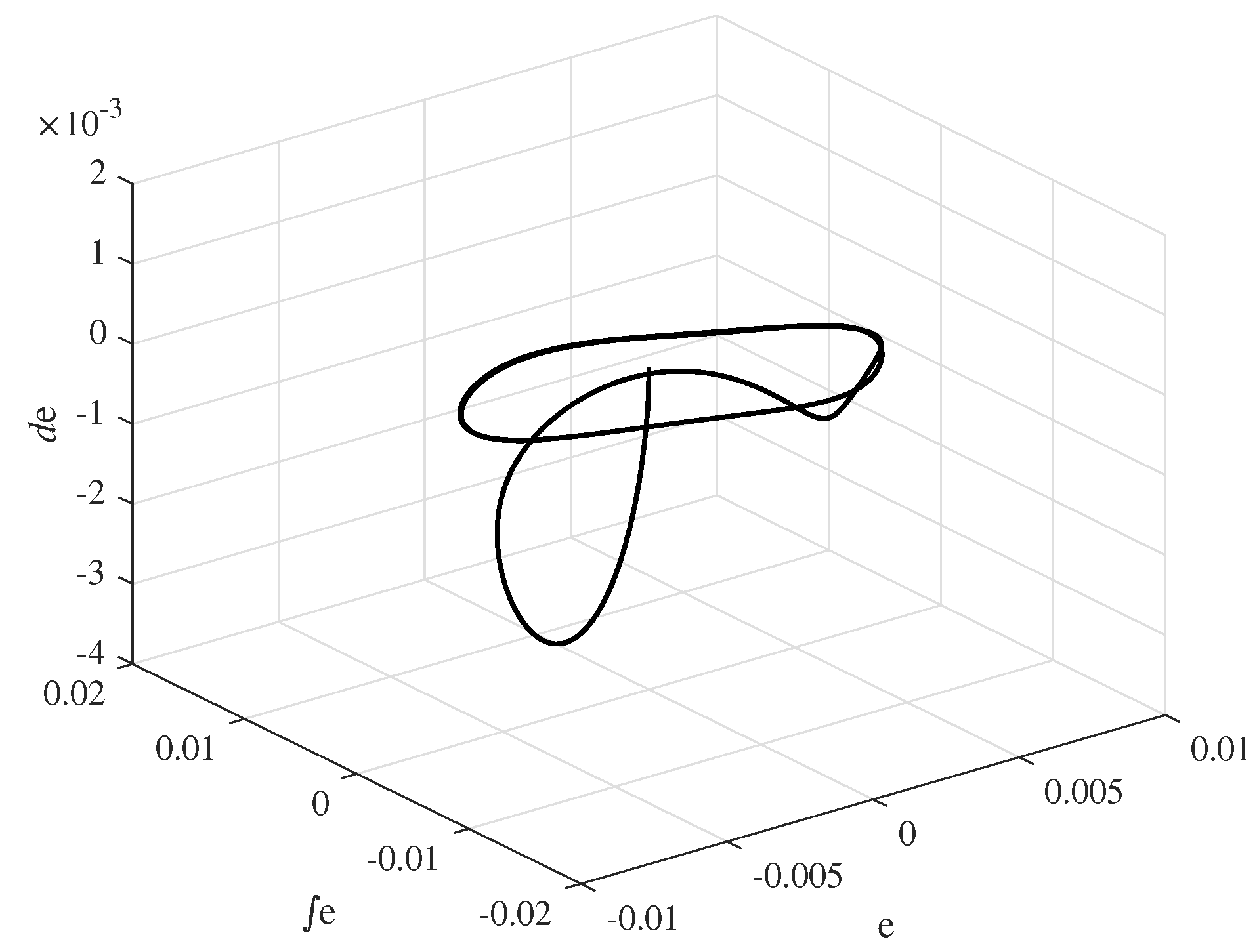
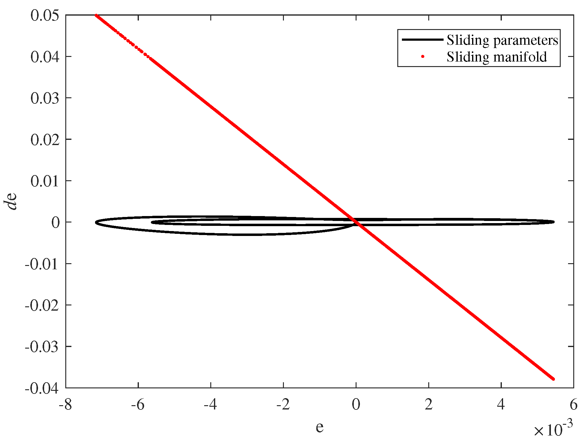
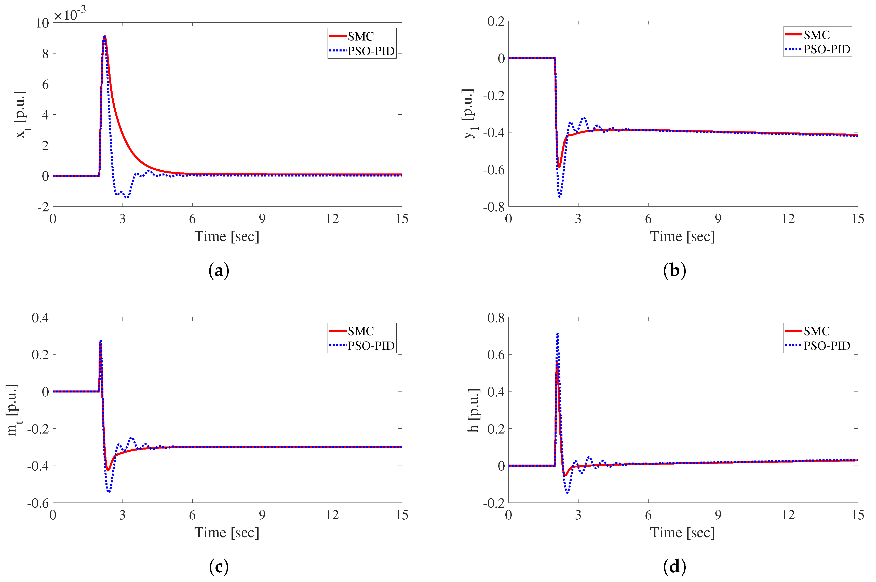
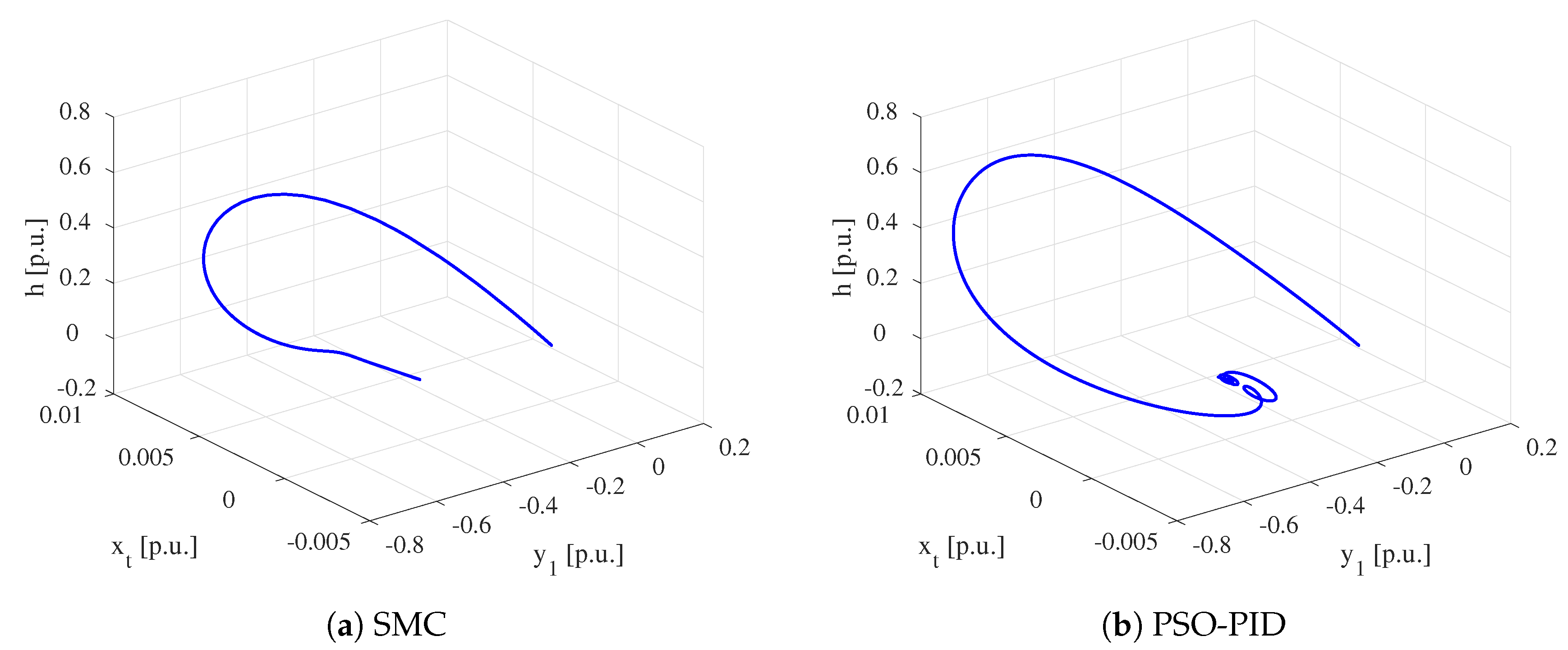
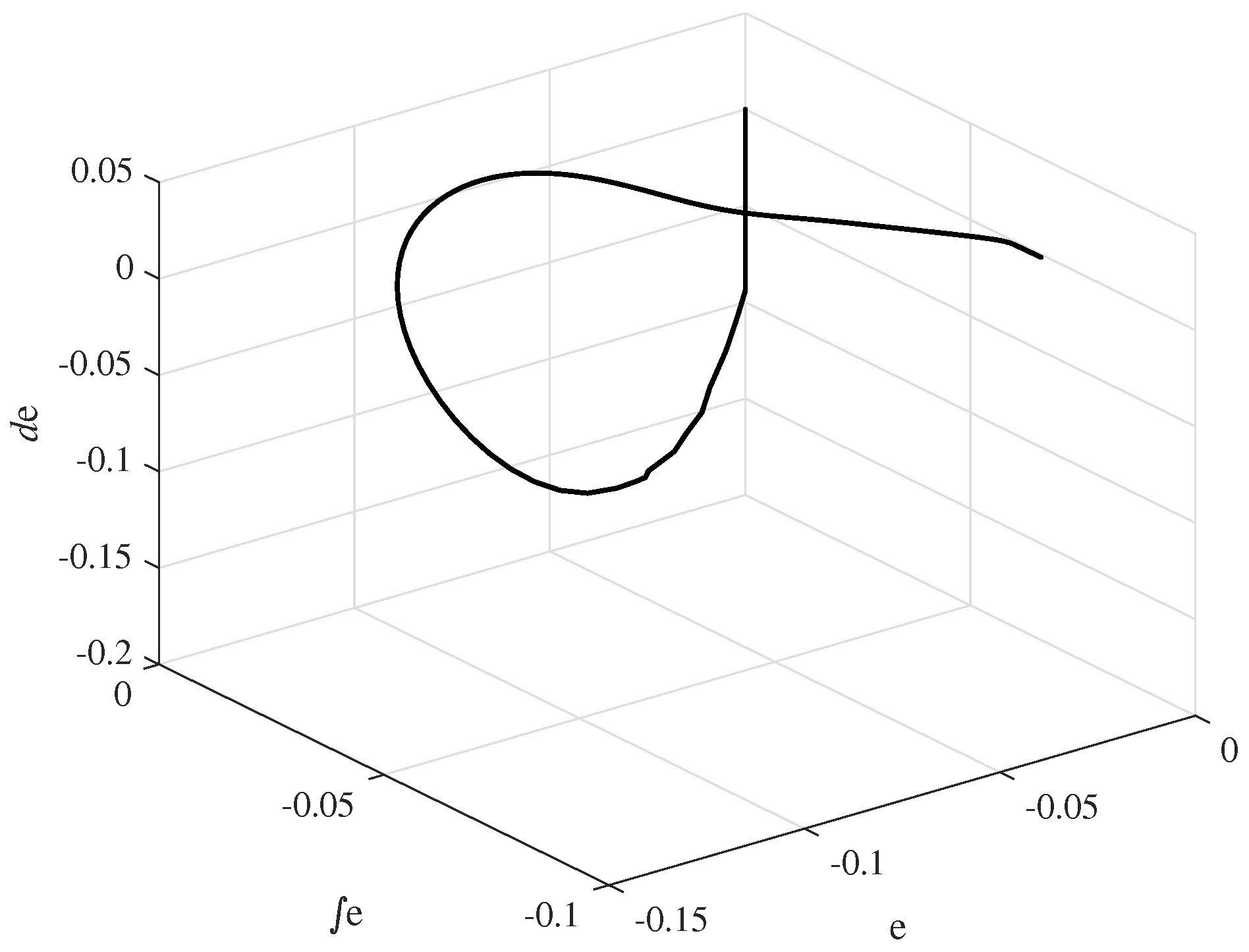
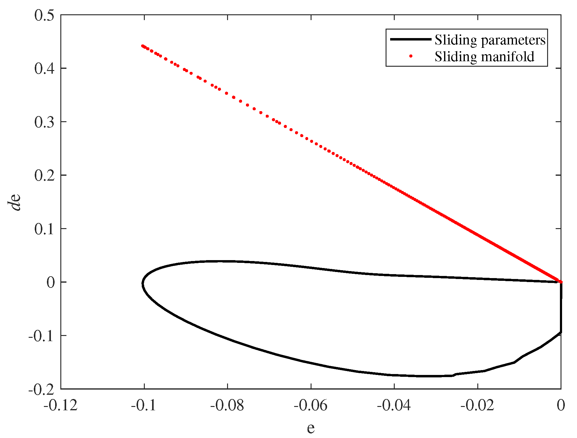
By optimizing the parameters of SMC control law, the hydraulic turbine system can be stabilized at a target turbine speed. At first, the HTGS operates at rated work condition for two seconds. Then, considering a $5\%$ decrease in rated speed, both PSO-PID governor and SMC governor are utilized to solve the case. The PSO tuned gains of the PID governor are set as: $k_p=14.4928$, $k_i=1.4412$ and $k_d=2.6913$, while the parameters of SMC governor are set as: ${\lambda }_p=10.194$, ${\lambda }_i=0.9222$, ${\lambda }_d=2.9653$, $\eta =0.05$, $\delta =0.02$ and $k=5$. Finally, the comparison results of waveforms about key state variables, $x_t$, $y_1$, $m_t$ and h are shown in Figure 3; the PSO-PID and SMC governed systems’ ternary phase diagrams of $y_1$-$x_t$-h are shown in Figure 4; a space phase diagram about sliding parameters e, $\int e$ and $de$, and its projection, a plain space phase diagram with setting sliding manifold, are shown in Figure 5 and Figure 6, respectively.

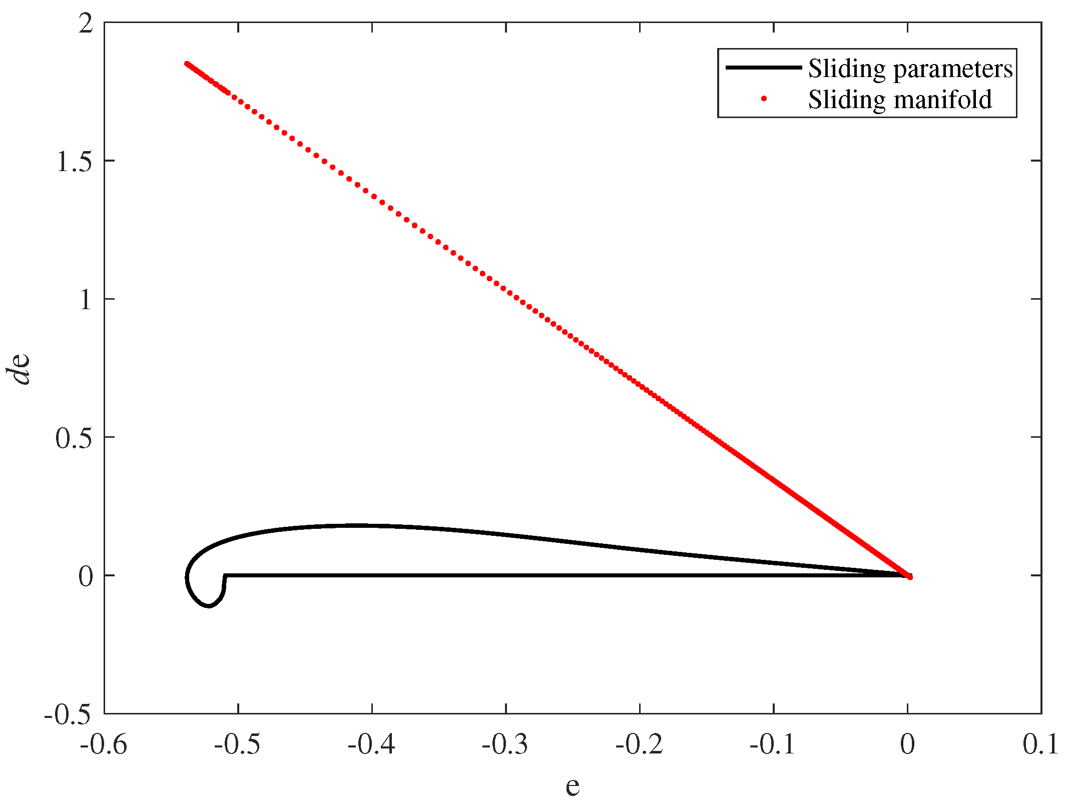
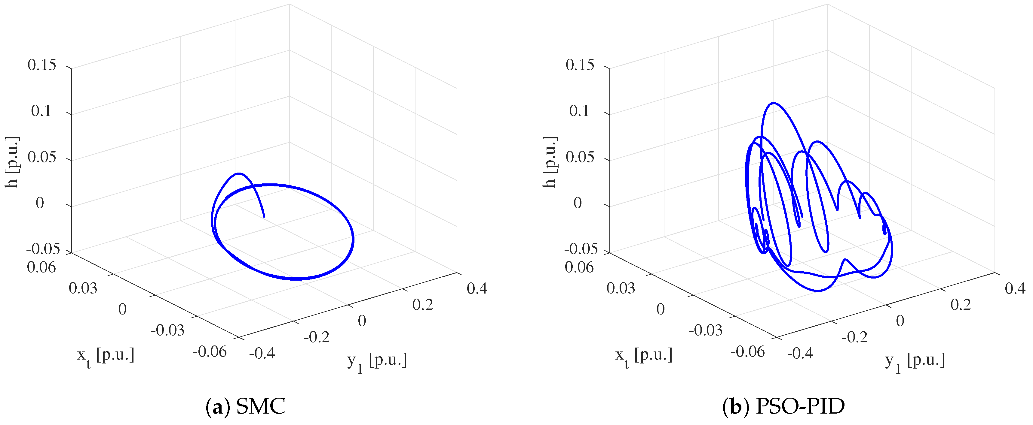
From Figure 3, with SMC acted, $x_t$ stabilizes at target turbine speed promptly without overshoot and vibration around the target speed compared with a PSO-PID governor. In addition, according to responses of all state variables, another significant advantage is the smoothness when states approach the equilibrium point, which is good for equipment maintenance due to less impact. From Figure 4, the $y_1$, $x_t$ and h under SMC tend to be stable more straightforward and less dispersed than the PSO-PID governor, which indicates that SMC is capable of keeping the system steady promptly. From Figure 5 and Figure 6, sliding parameters converge to setting manifold and stay stable in finite time.

4.2. Periodic Turbine Speed Trajectory Tracking

An extreme speed disturbance, cosine wave with $2\%$ amplitude of rated speed, is chosen as a test for tacking and latency suppressing ability of designed SMC controller. PSO-PID governor gains are tuned as: $k_p=17.0863$, $k_i=84.2919$, $k_d=3.7834$ while SMC governor parameters are set as: ${\lambda }_p=3.4141$, ${\lambda }_i=9.1297$, ${\lambda }_d=0.4899$, $\eta =4$, $\delta =0.1$, $k=9$. The comparison waveforms of $x_t$, $y_1$, $m_t$ and h are shown in Figure 7; ternary phase diagrams of $y_1$-$x_t$-h are shown in Figure 8; a space phase diagram of sliding parameters and a plain space phase diagram with setting sliding manifold are shown in Figure 9 and Figure 10.

From Figure 7, it shows an extraordinary periodic orbit tracking ability for SMC control law with each state controlled in periodic and vibration suppressed. However, under PSO-PID, the responses of state variables show significant vibration, especially water pressure in the wicket gate h, which makes a difference to operation safety. The diffused swirling trajectory governed by PSO-PID in Figure 8 also implies that the system is beyond control. However, governed by SMC, the clear occurrence of a limit cycle indicates that $y_1$, $x_t$ and h are in regular periodic motion. In Figure 9 and Figure 10, sliding parameters are revolving around the body-centered, which is zero steady error point.

4.3. Load Disturbance Response Testing

In practice, load disturbance is a frequently met operation requiring high-level flexibility and robust regulation capability to maintain grid stability [6,39]. Considering $30\%$ load shedding as the case, PSO-PID governor gains are tuned as: $k_p=25.8528$, $k_i=52.2091$, $k_d=4.464$ while SMC governor parameters are given as: ${\lambda }_p=11$, ${\lambda }_i=8$, ${\lambda }_d=2.5$, $\eta =0.6$, $\delta =0.02$, $k=10$. The comparison waveforms of $x_t$, $y_1$, $m_t$ and h are listed in Figure 11; ternary phase diagrams of $y_1$-$x_t$-h are shown in Figure 12; a space phase diagram of sliding parameters and its projection are presented in Figure 13 and Figure 14.

From the state variables responses in Figure 11 and ternary phase diagram in Figure 12, the SMC has the capability to cope with load disturbance with less overshoot and vibration compared to PID. In addition, it drives states to a steady constant point more directly rather than swirling around the steady point. According to sliding parameters’ trajectory, the system finally converges to setting manifold within a finite time and remains stable. In addition, the gains of PSO-PID controller are too big to achieve in real-time application.

4.4. Robustness Simulation against System Uncertainties

The above simulations are discussed under the situation when system uncertainties are not considered. However, the practical applications demonstrate that a variety of uncertainties, including measurement uncertainties, system intrinsic and external disturbances, exert considerable influences on hydraulic units’ operation. In addition, many studies are working on modeling and reducing these undesired and undetected uncertainties [23,24]. In this way, the robustness testing against disturbances is critical to any governor design. In this section, sine and cosine waves are chosen to model the disturbances in the conduit system, as well as random noises being adopted to model the noises in servomechanism and turbine speed. The uncertainty terms are defined as follows:

$$\begin{array}{c}{d}_1=0.01sin\left(t\right),d_2=-0.01sin\left(t\right),d_3=0.01cos\left(t\right),\\ d_4=r,d_5=-0.01cos\left(t\right),d_6=r,\end{array}$$

(32)

where r is random noise in finite range $\left[-0.01,0.01\right]$.

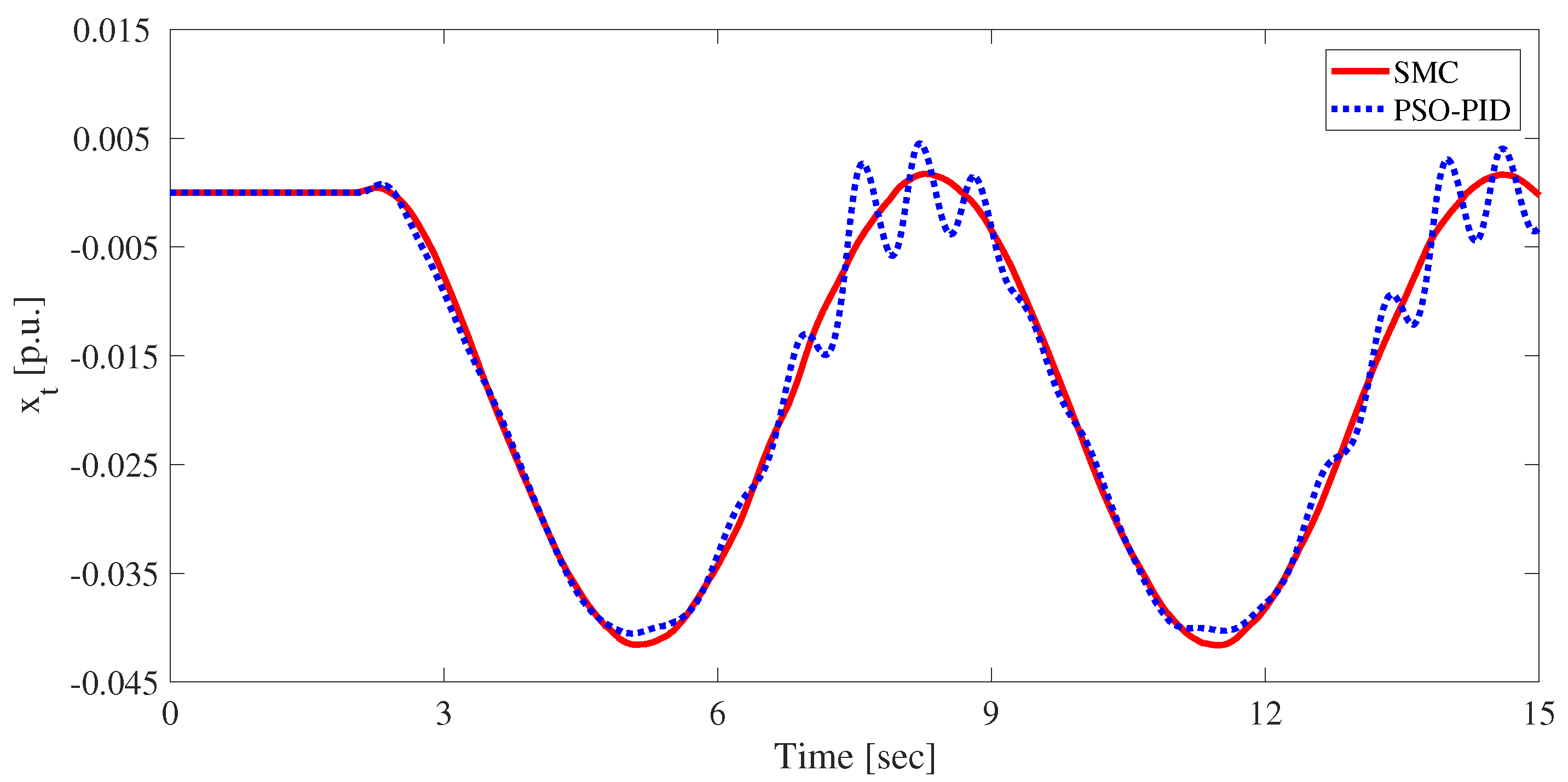
It uses the same experimental conditions under a cosine wave speed disturbance with $2\%$ amplitude of rated speed, and simulation results are represented in Figure 15.

Compared to PSO-PID control law, the SMC governor forces $x_t$ to target orbit without fluctuation undergoing system uncertainties and random noises, which indicates the strong robustness of SMC governor when facing undetected disturbances acted on HTGS. It shows that, by tuning the amplitude of switch function, the uncertainties are fully suppressed.

5. Conclusions

In this paper, a novel SMC regulating strategy with proportional-integral-derivative sliding manifold is proposed and applied to a highly coupled state variables HTGS. The stability of HTGS adopting SMC is fully discussed. By adopting exponential reaching law and setting proper boundary layer, the designed SMC method fastens the converging time and keeps the system stable at a desired state with chattering suppressed. The author suggests that an integral term is necessary to reduce the latency caused by anti-regulation features of nonlinear HTGS. To demonstrate the governor’s regulating performance, three frequently met operating conditions are simulated, compared with a PSO-PID governor using the elimination mechanism. Results imply that HTGS with SMC presents satisfactory performance and smooth responses when facing varying working conditions, which gives a bright picture of modeling and designing new regulating techniques for HTGS. Finally, the strong robustness of SMC is analyzed. In addition, future investigation of SMC regulating strategy should be focused on handling multiple hydraulic transients and fault conditions occurring in real-time application to demonstrate its regulating ability combining a more accurate nonlinear model in the situation of large fluctuation. Moreover, due to the proposed SMC method being frequency-primed control, the strong robustness mainly occurs on turbine speed response. The robustness on other key state variables should also be considered in future SMC design.

References

- Feng, Z.K.; Niu, W.J.; Cheng, C.T. China’s large-scale hydropower system: Operation characteristics, modeling challenge and dimensionality reduction possibilities. Renew. Energy 2019, 136, 805–818. [Google Scholar] [CrossRef]
- Shivarama Krishna, K.; Sathish Kumar, K. A review on hybrid renewable energy systems. Renew. Sustain. Energy Rev. 2015, 52, 907–916. [Google Scholar] [CrossRef]
- Yang, W.; Norrlund, P.; Bladh, J.; Yang, J.; Lundin, U. Hydraulic damping mechanism of low frequency oscillations in power systems: Quantitative analysis using a nonlinear model of hydropower plants. Appl. Energy 2018, 212, 1138–1152. [Google Scholar] [CrossRef]
- Kishor, N.; Saini, R.P.; Singh, S.P. A review on hydropower plant models and control. Renew. Sustain. Energy Rev. 2007, 11, 776–796. [Google Scholar] [CrossRef]
- Guo, W.; Yang, J. Modeling and dynamic response control for primary frequency regulation of hydro-turbine governing system with surge tank. Renew. Energy 2018, 121, 173–187. [Google Scholar] [CrossRef]
- Zhou, J.; Zhang, Y.; Zheng, Y.; Xu, Y. Synergetic governing controller design for the hydraulic turbine governing system with complex conduit system. J. Frankl. Inst. 2018, 355, 4131–4146. [Google Scholar] [CrossRef]
- Guo, W. Nonlinear disturbance decoupling control for hydro-turbine governing system with sloping ceiling tailrace tunnel based on differential geometry theory. Energies 2018, 11, 3340. [Google Scholar] [CrossRef]
- Li, C.; Zhang, N.; Lai, X.; Zhou, J.; Xu, Y. Design of a fractional-order PID controller for a pumped storage unit using a gravitational search algorithm based on the Cauchy and Gaussian mutation. Inf. Sci. 2017, 396, 162–181. [Google Scholar] [CrossRef]
- Nagode, K.; Skrjanc, I. Modelling and internal fuzzy model power control of a Francis water turbine. Energies 2014, 7, 874–889. [Google Scholar] [CrossRef]
- Kishor, N.; Singh, S.P. Simulated response of NN based identification and predictive control of hydro plant. Exp. Syst. Appl. 2007, 32, 233–244. [Google Scholar] [CrossRef]
- Li, X.; Li, M.; Sun, J.; Hu, W.; Xu, F. Nonlinear adaptive decentralized stabilizing control for the hydraulic turbines’ governor system. In Proceedings of the 2011 International Conference on Advanced Power System Automation and Protection, Beijing, China, 16–20 October 2011; Volume 3, pp. 1913–1917. [Google Scholar] [CrossRef]
- Zhu, W.; Zheng, Y.; Dai, J.; Zhou, J. Design of integrated synergetic controller for the excitation and governing system of hydraulic generator unit. Eng. Appl. Artif. Intell. 2017, 58, 79–87. [Google Scholar] [CrossRef]
- Izquierdo, J.; Iglesias, P.L. Mathematical modelling of hydraulic transients in simple systems. Math. Comput. Model. 2002, 35, 801–812. [Google Scholar] [CrossRef]
- Kishor, N.; Singh, S.P.; Raghuvanshi, A.S. Dynamic simulations of hydro turbine and its state estimation based LQ control. Energy Convers. Manag. 2006, 47, 3119–3137. [Google Scholar] [CrossRef]
- Fang, H.Q.; Shen, Z.Y. Modeling and simulation of hydraulic transients for hydropower plants. In Proceedings of the 2005 IEEE/PES Transmission & Distribution Conference & Exposition: Asia and Pacific, Dalian, China, 18 August 2005; Volume 2005, pp. 1–4. [Google Scholar] [CrossRef]
- Hydraulic turbine and turbine control models for system dynamic studies. IEEE Trans. Power Syst. 1992, 7, 167–179. [CrossRef]
- Zhou, J.; Cai, F.; Wang, Y. New elastic model of pipe flow for stability analysis of the governor-turbine-hydraulic system. J. Hydraul. Eng. 2011, 137, 1238–1247. [Google Scholar] [CrossRef]
- Chen, D.; Ding, C.; Ma, X.; Yuan, P.; Ba, D. Nonlinear dynamical analysis of hydro-turbine governing system with a surge tank. Appl. Math. Model. 2013, 37, 7611–7623. [Google Scholar] [CrossRef]
- Sanathanan, C.K. Accurate low order model for hydraulic turbine-penstock. IEEE Trans. Energy Convers. 1987, EC-2, 196–200. [Google Scholar] [CrossRef]
- Zhang, H.; Chen, D.; Xu, B.; Wang, F. Nonlinear modeling and dynamic analysis of hydro-turbine governing system in the process of load rejection transient. Energy Convers. Manag. 2015, 90, 128–137. [Google Scholar] [CrossRef]
- Shen, Z.Y. Hydraulic Turbine Regulation; China Waterpower Press: Beijing, China, 1998. (In Chinese) [Google Scholar]
- Liu, J.; Wang, X. Advanced Sliding Mode Control for Mechanical Systems Design, Analysis and MATLAB Simulation; Springer: Berlin/Heidelberg, Germany, 2012. [Google Scholar] [CrossRef]
- Konidaris, D.N.; Tegopoulos, J.A. Investigation of oscillatory problems of hydraulic generating units equipped with Francis turbines. IEEE Trans. Energy Convers. 1997, 12, 419–425. [Google Scholar] [CrossRef]
- Nguyen, C.M.; Pathirana, P.N.; Trinh, H. Robust observer and observer-based control designs for discrete one-sided Lipschitz systems subject to uncertainties and disturbances. Appl. Math. Comput. 2019, 353, 42–53. [Google Scholar] [CrossRef]
- Pradhan, S.; Singh, B.; Panigrahi, B.K.; Murshid, S. A composite sliding mode controller for wind power extraction in remotely located solar PV-wind hybrid system. IEEE Trans. Ind. Electron. 2019, 66, 5321–5331. [Google Scholar] [CrossRef]
- Incremona, G.P.; Cucuzzella, M.; Ferrara, A. Adaptive suboptimal second-order sliding mode control for microgrids. Int. J. Control 2016, 89, 1849–1867. [Google Scholar] [CrossRef] [Green Version]
- Wan, L.; Su, Y.; Zhang, H.; Tang, Y.; Shi, B. Global fast terminal sliding mode control based on radial basis function neural network for course keeping of unmanned surface vehicle. Int. J. Adv. Robot. Syst. 2019, 16, 12. [Google Scholar] [CrossRef]
- Precup, R.E.; Radac, M.B.; Roman, R.C.; Petriu, E.M. Model-free sliding mode control of nonlinear systems: Algorithms and experiments. Inf. Sci. 2017, 381, 176–192. [Google Scholar] [CrossRef]
- Yuan, X.; Chen, Z.; Yuan, Y.; Huang, Y.; Li, X.; Li, W. Sliding mode controller of hydraulic generator regulating system based on the input/output feedback linearization method. Math. Comput. Simul. 2016, 119, 18–34. [Google Scholar] [CrossRef]
- Wu, F.; Li, F.; Chen, P.; Wang, B. Finite-time control for a fractional-order nonlinear, HTGS. IET Renew. Power Gener. 2019, 13, 633–639. [Google Scholar] [CrossRef]
- Chen, Z.; Yuan, X.; Yuan, Y.; Lei, X.; Zhang, B. Parameter estimation of fuzzy sliding mode controller for hydraulic turbine regulating system based on HICA algorithm. Renew. Energy 2019, 133, 551–565. [Google Scholar] [CrossRef]
- Yan, D.; Zhuang, K.; Xu, B.; Chen, D.; Mei, R.; Wu, C.; Wang, X. Excitation current analysis of a hydropower station model considering complex water diversion pipes. J. Energy Eng. 2017, 143, 04017012. [Google Scholar] [CrossRef]
- Chang, L.Y.; Chen, H.C. Linearization and input-output decoupling for nonlinear control of proton exchange membrane fuel cells. Energies 2014, 7, 591–606. [Google Scholar] [CrossRef]
- Xiong, L.; Li, P.; Li, H.; Wang, J. Sliding mode control of DFIG wind turbines with a fast exponential reaching law. Energies 2017, 10, 19. [Google Scholar] [CrossRef]
- Precup, R.E.; David, R.C. Chapter 2—Nature-inspired algorithms for the optimal tuning of fuzzy controllers. In Nature–Inspired Optimization Algorithms for Fuzzy Controlled Servo Systems; Butterworth-Heinemann: Oxford, UK, 2019; pp. 55–80. [Google Scholar]
- Lei, G. Application improved particle swarm algorithm in parameter optimization of hydraulic turbine governing systems. In Proceedings of the 2017 IEEE 3rd Information Technology and Mechatronics Engineering Conference (ITOEC), Chongqing, China, 3–5 Octorber 2017; pp. 1135–1138. [Google Scholar] [CrossRef]
- Fang, H.Q.; Shen, Z.Y. Optimal hydraulic turbogenerators PID governor tuning with an improved particle swarm optimization algorithm. Proc. Chin. Soc. Electr. Eng. 2005, 25, 120–124. (In Chinese) [Google Scholar]
- Martins, F.G. Tuning PID controllers using the ITAE criterion. Int. J. Eng. Educ. 2005, 21, 867–873. [Google Scholar]
- Trivedi, C.; Agnalt, E.; Dahlhaug Ole, G. Experimental investigation of a Francis turbine during exigent ramping and transition into total load rejection. J. Hydraul. Eng. 2018, 144, 04018027. [Google Scholar] [CrossRef]