Adaptive Unscented Kalman Filter with Correntropy Loss for Robust State of Charge Estimation of Lithium-Ion Battery


1
School of Microelectronics, Xi’an Jiaotong University, Xi’an 710049, China
2
Department of Technology, Xi’an Aerosemi Technology Co., Ltd., Xi’an 710077, China
3
School of Automation and Information Engineering, Xi’an University of Technology, Xi’an 710048, China
*
Authors to whom correspondence should be addressed.
Energies 2018, 11(11), 3123; https://doi.org/10.3390/en11113123
Submission received: 6 October 2018
/
Revised: 1 November 2018
/
Accepted: 10 November 2018
/
Published: 12 November 2018
(This article belongs to the Special Issue Battery Storage Technology for a Sustainable Future)
Abstract
:As an effective computing technique, Kalman filter (KF) currently plays an important role in state of charge (SOC) estimation in battery management systems (BMS). However, the traditional KF with mean square error (MSE) loss faces some difficulties in handling the presence of non-Gaussian noise in the system. To ensure higher estimation accuracy under this condition, a robust SOC approach using correntropy unscented KF (CUKF) filter is proposed in this paper. The new approach was developed by replacing the MSE in traditional UKF with correntropy loss. As a robust estimation method, CUKF enables the estimate process to be achieved with stable and lower estimation error performance. To further improve the performance of CUKF, an adaptive update strategy of the process and measurement error covariance matrices was introduced into CUKF to design an adaptive CUKF (ACUKF). Experiment results showed that the proposed ACUKF-based SOC estimation method could achieve accurate estimate compared to CUKF, UKF, and adaptive UKF on real measurement data in the presence of non-Gaussian system noises.
1. Introduction
Reliable and accurate state of charge (SOC) estimate of lithium-ion battery plays a crucial role in battery management systems (BMS) [1,2,3,4,5,6]. At present, SOC estimate methods based on Kalman filter (KF) are gaining great interest due to their excellent convergence performance and initial value insensitivity. As a data processing algorithm with autoregressive optimal characteristic, KF can make the best estimate of the minimum variance in the system state. For SOC estimate, the traditional linear KF-aware algorithms can not only overcome the error accumulation effect of the coulomb counting method, but it also does not depend on an accurate initial SOC value [3,4]. However, the accuracy of this method relies on the establishment of a battery equivalent circuit mode (ECM), and some physical properties of the battery model are nonlinear [5,6]. For this reason, the extended KF (EKF) algorithm is proposed in this paper using first-order Taylor series expansion to improve the performance of conventional KF algorithms, which implements recursive filtering by linearizing nonlinear functions. Unfortunately, EKF may produce large estimation errors or may even diverge when the system nonlinearity is strong. To circumvent first-order approximation errors of EKF, the UKF algorithm was developed by applying nonlinear system equations to the standard KF by means of unscented transformation (UT) naturally [7,8,9,10,11].
Compared with EKF, UKF can achieve higher accuracy for solving nonlinear estimation problems in a wider application range. Therefore, more and more UKF and SOC estimate methods based on its variations have been developed in recent years [12,13]. In Reference [12], a modified ECM model with the impact of different current rates and SOC on the battery internal resistance was presented, and the UKF algorithm was introduced to estimate SOC. An adaptive UKF (AUKF) and least-square support vector machines (LSSVM)-based accurate SOC estimation algorithm for lithium polymer battery was proposed in Reference [13] in which AUKF and LSSVM were used to accurately establish the battery model with limited initial training samples. Li et al. proposed a wavelet transform-adaptive UKF approach for SOC estimation of LiFePo4 battery [14]. Considering SOC estimation in uncertain operating environments, the joint SOC estimation method was proposed in Reference [15], where the H-infinity filter was used to estimate battery model parameters, while SOC was estimated using UKF. In the studies, both the process and the observation noises of the system nonlinear dynamic models were assumed to be Gaussian when developing a SOC estimation method. However, BMS usually suffers from unexpected sensing of noises that may not follow Gaussian distributions in practice because of the uncertainties of the system [16,17,18], meaning the measurement errors of the voltage and current may obey non-Gaussian probability distributions. Therefore, the received measurements may be significantly biased because of non-Gaussian noise. Under this condition, traditional UKF-based SOC estimate methods will obtain biased estimation results. To address the state estimation issue under non-Gaussian noise cases, several robust UKF algorithms have been developed in the last few years. The GM-UKF [19] was proposed for power system state estimation that is able to filter out unknown Gaussian and non-Gaussian noises. As a robust cost function in information theoretic learning (ITL), correntropy loss [20] has been widely used to design different robust filters, such as sparse-aware correntropy filter [21], diffusion correntropy [22], and linear correntropy KF (CKF) [23]. For nonlinear estimation problems in impulsive noise environments, the extended CKF and the correntropy UKF (CUKF) were proposed in References [24,25,26,27,28].
At present, CUKF is widely used in nonstationary growth model estimation and signal processing. To the best of our knowledge, however, it has not been applied to handle SOC estimation for lithium ion when the system encounters non-Gaussian noises. Therefore, to overcome the drawback of SOC estimation based on traditional UKF under non-Gaussian situations, as well as inspired by the outstanding properties of CUKF, this paper aims to develop a robust SOC estimation method using CUKF. Although CUKF performs well in non-Gaussian cases, similar to UKF, it will only work under certain condition where the means and covariance matrices of the system process and measurement noises are assumed to be known at each time instant. However, for practical dynamical systems, these may be difficult to obtain because both noises depend heavily on the actual operating conditions of the system and change from time to time [19]. For this reason, an adaptive update scheme was introduced into CUKF to adjust the process and measurement noise covariance matrices adaptively, and a novel adaptive CUKF (ACUKF)-based SOC estimation method was further developed to suppress the influence of non-Gaussian measurement noise. The proposed method was implemented and tested on lithium ion with the current profiles. The experimental results demonstrated that the proposed ACUKF method could achieve higher estimation accuracy and fast convergence for SOC estimation in comparison to the conventional UKF and adaptive UKF.
The remainder of this paper is organized as follows. Section 2 describes the battery model structure selected for study in this paper. Section 3 introduces the SOC estimation method based on adaptive CUKF. The SOC estimation method via ACUKF is validated using experimental data in Section 4. Finally, Section 5 concludes with a summary of the main findings of this paper.
2. Equivalent Circuit Model and Parameter Identification
The ECM is the foundation of KF-based SOC estimate methods for lithium ion in BMS. It uses simple elements such as resistors and capacitors to model the charging and discharging behavior of lithium-ion batteries [29]. The available lithium-ion battery charging strategies usually fall into three categories depending on the mathematical models utilized [30]. In this section, the overall framework of ECM and its parameters identification process will be introduced.
2.1. Two-Order R-C ECM
A reliable ECM is a prerequisite for accurate SOC estimation. Various ECMs are now extensively utilized in SOC estimate studies, including Thevenin model [31], Rint model [32], resistor–capacitor (R-C) model [33], Partnership for a New Generation of Vehicles (PNGV) model [34], fractional-order battery model [35], and so on. Among them, R-C network is one of important models because it can accurately capture the battery dynamics and can be easily implemented in real-time applications. According to the report in Reference [29], the model accuracy is not always improved by increasing the order of the R-C network, and the first- and second-order R-C models are the best choice owing to their balance of accuracy and reliability for lithium-ion batteries. Therefore, the two-order R-C model was selected as the ECM in this work, as shown in Figure 1.
In this model, denotes the battery’s Ohmic resistance, which represents the instantaneous voltage drop during the battery charge/discharge process. Two R-C networks are used to model the relaxation effects of battery charge/discharge process. The and branch imitates the short-term transient response of battery, whereas the long-term transient response is modeled by and . The represents the battery’s open circuit voltage (OCV), which is usually a nonlinear function of SOC. denotes the battery terminal voltage, and is the load current with a positive value at discharge and a negative value at charge. and are the short- and long-time transient voltage responses for charging/discharging, respectively. Using the Kirchhoff’s circuit laws, the electrical behavior of the 2-R-C model can be expressed as follows:
In this model, the parameter vectors (R0, Rs, Rd, Cs, and Cd) should be experimentally identified efficiently to increase the SOC accuracy in real-time application. The following parameter identification process is shown on actual data taken from the website of the “Battery Management Systems, Volume II: Equivalent-Circuit” course [36].
2.2. SOC-OCV Relationship
As the terminal voltage of battery at charge equilibrium condition, the OCV is directly dependent on SOC value. To obtain the nonlinear functional relationship between OCV and SOC, the OCV test was conducted using the lithium-ion battery as a case study. In this study, the hysteresis effect was neglected. The discharge characteristic experiment with 1C rate was conducted for the battery, and the test temperature was kept at 25 °C. The 8th degree polynomial equation was employed to fit the relationship accurately using the experimental data because it had shown better performance than the 7th degree one in References [15,37,38]. With 18 pairs of OCV and SOC data, the OCV–SOC relationship was determined by the polynomial fitting method as follows:
2.3. Identification of Model Parameters
In this subsection, we identify the parameters (R0, Rs, Rd, Cs, and Cd) using the off-line method. Under the same temperature conditions, a hybrid pulse current profile was loaded to get the battery model parameters. Data obtained from the test on LiFePO4 battery in Reference [34] was used in this work. The key specifications of a LiFePO4 battery selected for the experiment were as follows: The nominal capacity of the battery was 5 Ah, nominal voltage was 3.5 V, and maximum continuous discharge current was 8.5 A. The batteries were placed in the temperature chamber, and the temperature of the cell was measured. The current, voltage, and SOC were sampled at 1 Hz and are plotted in Figure 3a–c. The experiments in Section 4 were conducted using these data to verify the performance of the novel SOC estimate method proposed in this work.
(1) Ohmic resistance R0
The resistive and capacitive parameters of the battery ECM can be identified by data obtained from the unidirectional pulse charging test and the unidirectional pulse discharging test described at the beginning of this section. Ohmic resistance is the main cause of lithium battery current load voltage changes, and its identification calculation can be obtained according to the terminal variation. According to the Ohm’s law of equation [39] we get the following:
from this, we can deduce .
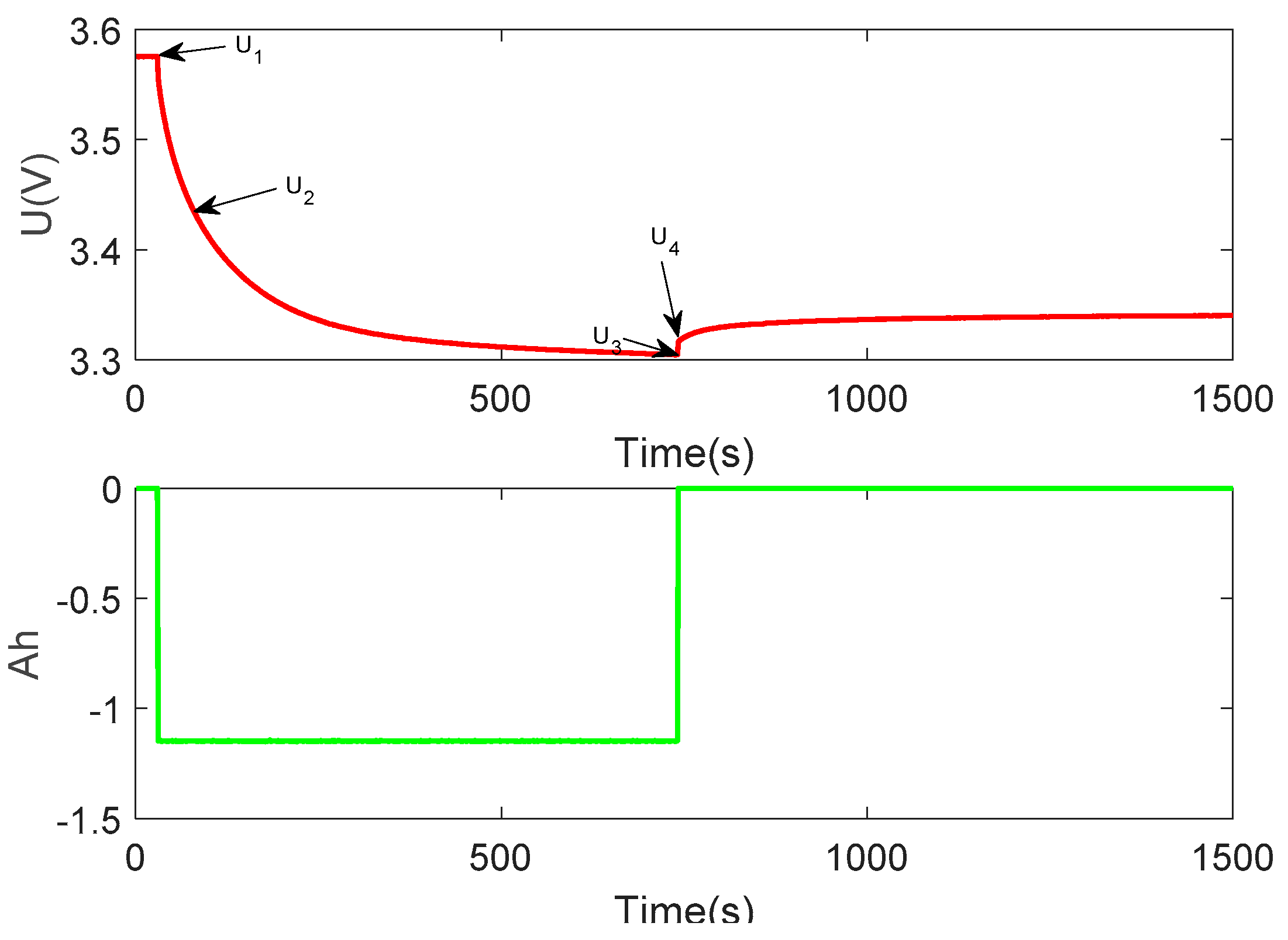
Figure 4 is the terminal voltage response curve of unidirectional pulse discharge sequence. In the terminal voltage response curve, the instantaneous variation of the voltage at the beginning and end of the pulse discharge current is mainly caused by the Ohmic resistance R0 because of the very short pulse discharge time, while SOC changes little before and after pulse discharge. Once the discharge current is stopped, the terminal voltage will drop immediately. It must be noted that the voltage and of the capacitors and will not suddenly change at the moment of starting the discharge. Then, Ohmic resistance can be found from numerous of the terminal voltage at the moment of starting the discharge. Thus, we can calculate the Ohmic resistance [40]:
(2) Polarization resistance–capacitance parameters
The exponential fitting approach is employed to identify the model parameters Rs, Rd, Cs, and Cd. The time constant , should be computed first. Using the identified time constant, the details identification of the , , , and can then be introduced. During pulse discharge end static period, R-C network is zero input response; then, the terminal voltage can be represented as follows:
where is the initial value of the voltage at the two ends of the network, and is the initial value of the voltage at the two ends of the network. According to Equation (7), we can perform the second-order exponential fitting of the terminal voltage response by the following expression:
Here, are unknown coefficients, and we can obtain the value of them by least-square fitting method. Then, the parameters can be identified further by the following methodology.
Using Kirchhoff’s circuit laws, the circuit dynamics of the RC network combining and can be expressed as follows:
where , then, the above equation can be written as follows:
Solving the differential equation yields, we get the following:
In like manner, we have the following:
Further, we have the following:
Then, from Equations (11) and (13), the resistances Rs and Rd are determined by the following equations:
Now, the values of and can be computed from .
Then, the parameter identification is completed and the results are given in Table 1.
(3) Parameter validation test
In order to verify the correctness of the battery equivalent circuit model and parameter identification method, it was necessary to compare the measured battery terminal voltage with the terminal voltage obtained by the model. The output of the model was obtained by the following equation:
Figure 5a gives the actual voltage and the model output voltage results, and Figure 5b is the difference between them. From this result, we can observe that the model output voltage is identical with the actual voltage, and it implies availability of the parameters obtained by the process above for the selected battery. However, we can also observe that the absolute difference increases over 0.2 V during charge/discharge stage. There are two probable reasons for this phenomenon: (1) The dynamic characteristic of charge/discharge leads to fluctuation. (2) There is noise in the dynamic charge–discharge process. This seems to be a critical flaw of the calculated parameters, and we will focus on this issue in future research.
3. Adaptive Correntropy UKF for SOC
In this section, we introduce a novel SOC estimation approach using correntropy UKF with adaptive update of process and measurement error covariance matrices.
3.1. Correntropy Loss
As a nonlinear similarity measure, correntropy has been proposed in information theoretical learning (ITL) framework where the conventional concepts of second-order statistics (covariance, L2 distances, correlation functions) are substituted by scalars and functions with information theoretic underpinnings—entropy, mutual information, and correntropy, respectively [41]. For two random variables and , its definition is as follows:
where denotes the expectation operator, is a kernel function with kernel width , and represents the joint distribution function. In general, the data distribution is not obtained and only a finite number of samples are available, hence the sample estimator of correntropy is used as follows:
The Gaussian kernel is usually used in correntropy and given by the following equation:
where denotes the error of two random variables. As a local similarity criterion, correntropy is very useful for non-Gaussian cases, especially for measurement noise with large outlier. It is always bounded for any distribution and robust with respect to impulsive noises (or outliers) [42,43]. correntropy loss is aimed at maximizing correntropy between a variable and its estimator, which has been successfully applied in designing robust adaptive filters [21,22,23,24,25,26,27,28].
3.2. UKF with Correntropy Loss
The KF is a computing tool that can provide an efficient recursive means for estimating the states of a process by minimizing the MSE, which is used as an optimal criterion under Gaussian assumption. Unfortunately, this condition may still not hold true in real world. Therefore, several novel KFs via a substitute criterion have been developed to improve the robustness of the conventional KF. correntropy loss, as a simple and efficient criterion, has been employed to design different kinds of KFs, such as correntropy KF [23,24], correntropy EKF [25], and CUKF [26,27,28]. In this work, we focused on the development of a novel SOC estimate method based on the proposed adaptive CUKF. CUKF and the adaptive update scheme of the process and measurement noises covariance matrices for CUKF are introduced in this section.
The following state-space equation model was used to introduce CUKF from Reference [26].
State equation:
Measurement equation:
where denotes the state-space model, is the measurement model, denotes state variable, represents input variable, is output variable. and are process noise and measurement noise, respectively.
In general, CUKF also follows the structure of standard UKF using modified one-step estimation error covariance and measurement error covariance. The whole algorithm is given as follows:
Step1: A suitable kernel bandwidth and the initial state variable are first selected, then the initial state mean , is the covariance of the state estimate error defined by .
Step 2: Compute sigma points using and by the following equation:
where is the sth column of , is a scaling parameter used to reduce the prediction error, determines the spread of the sigma points around and is usually set to a small positive value, . The value of k is set to guarantee semipositive properties of the matrices and is set at 2 when the state variable is a single argument, while k = 3 − n when the state variable is multivariable. is the state estimation at time index i-1, and represents the related estimation error covariance matrix.
Step 3: Obtain the weight of the sigma point:
where is the weight of the sigma point mean, denotes the weight of the covariance, the free parameter , which can integrate into the prior information of random variable, and it is optimal when for Gaussian distribution.
Step 4: Obtain the mean and covariance of the one-step predicted state by the following equations:
Step 5: Computing of sigma point using and by the following equation:
Step 6: Obtain the mean and the cross-covariance matrix of the predicted measurement by the following equations:
Step 7: Get the pseudo measurement matrix by the following equation:
Step 8: Calculate the modified and as follows:
where is the lth elements of , and are from the following fixed-point equation with matrix form as follows:
where . In addition, we have the following:
Step 9: Obtain and calculate and through the following equations:
Remark 1:
According to Equations (36) and (37), we know that the difference between UKF and CUKF mainly lies inand. Due to the Gaussian kernel introduced by correntropy loss, CUKF will automatically adjust those two matrices in response to non-Gaussian signals. The detailed derive process for the state equation can be seen in Reference [26].
3.3. Adaptive Correntropy UKF
The process noise covariance and measurement noise are assumed to be known in CUKF. However, they are real time in general and may not be obtained prior in practice. Therefore, they should be updated with changes in time on the basis of some obtained prior knowledge. In recent years, different methods have been used to implement the adaptive estimation [44,45,46]. In this work, we use the covariance matching technique to estimate the covariance values to improve the robustness of CUKF. The realization process is detailed in the following:
where is the residual error of the measurement output, and denotes the residual error of the measurement output estimated by each sigma point. We can now give analysis of the method above.
According to Equation (21), we have the following:
Then, Equations (44) and (46) are the estimate of the . denotes the residual error covariance of the measurement, the mean of the sum of the residual error covariance can be estimate of the measurement noise covariance. According to Equation (11), we have the following
Further, from Equation (39), we obtain the following:
Due to
Thus,
When Equations (43) and (44) are introduced into CUKF, we can obtain the adaptive CUKF algorithm, which can overcome the drawback of CUKF and improve the estimate accurate by adjusting the covariance of the process and measurement noises.
3.4. ACUKF for SOC Estimation
In order to estimate SOC using the ACUKF, we substitute the state vector x in Equation (11) by the factor in ECM, which represents the total effect of system inputs u on the current system operation, such as SOC, and the measurable system output y is replaced by terminal voltage in Equation (12). w is the unmeasured “process noise” that affects the system state, and v is the measurement noise that does not affect the system state but can be reflected in the system output. f(x,u) and g(x,u) are functions specified by the particular used cell model. Then, discretizing Equations (1)–(3), we obtain the following:
where is the sampling interval, represents the SOC value at discretizing time k, and its discretizing form is as follows:
where is the total battery capacity.
The state variable of the systems usually comprises Equations (51), (52) and (54), while the terminal voltage in Equation (6) represents the model output measurement; the current is the input. To this end, the state and measurement equations with matrix form in discrete time can be expressed as follows:
4. Experiment Results and Discussion
We performed experiments to verify the effectiveness and feasibility of the proposed ACUKF for SOC estimation of lithium ion with respect to the database available in the research of the ECM data repository [36], and the true SOC was obtained by subtracting the net charge flow from the charge in a fully charged cell.
In general, the measurement data is usually not consistent with the original data due to the measurement error and observation error. Furthermore, these errors can also be seen from measurement noises. Therefore, in this work, we focused on the SOC estimation problem when the measurement data is affected by the noises with Gaussian and non-Gaussian cases. In order to make a quantitative comparison study of different SOC estimation methods, the mean square error (MSE), maximum absolute error (MAE), and root MSE (RMSE) were calculated according to the formula in Equations (57)–(59):
The performance of the proposed ACUKF for SOC estimation was compared with three other techniques—UKF, CUKF, and AUKF—under Gaussian and non-Gaussian environments.
4.1. Under Gaussian Noise
We first performed an experiment under Gaussian noise environments to evaluate the validation of the proposed method. Here, all the values of tuning parameters of each algorithm were selected by following the principle of obtaining optimal performance for them. The same free parameters of all algorithms were set at , k = 0, . The initial state was set at 70%, and the kernel width was selected as 2 for CUKF and ACUKF. We added the Gaussian noise with zero mean and variance 0.0001 as the state noise for state equation and selected another Gaussian noise with zero mean and variance 0.001 for measurement noise. The SOC estimate results are shown in Figure 6. From this result, one can observe that all the estimate methods performed well in this case, and the SOC estimate results of all methods were similar to each other. However, from the estimate errors in Figure 7, we see that differences still existed between them. In particular, the UKF and AUKF methods had larger initial error compared with CUKF and ACUKF. The MSE, RMSE, and MAE results of all methods are given in Table 2.
4.2. Under Non-Gaussian Noise
We know that non-Gaussian noises are common in real environments, so it is worthwhile to investigate the performance of the proposed method under the contamination of non-Gaussian noises. Two different cases for the system and measurement disturbances were considered to evaluate the SOC estimation performance of the proposed approach.
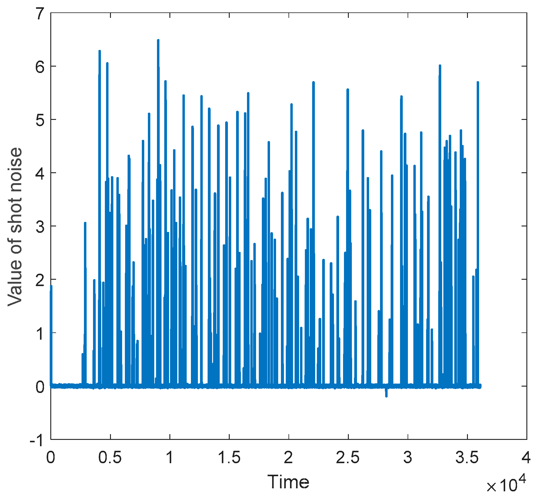
Case 1: In this case, the elements of and comprised Gaussian noise plus shot noise. The noise terms are represented as follows:
where , , , .
The shot noises applied to the first measurement are demonstrated in Figure 8; the shot noise used for was similar but is not shown here.
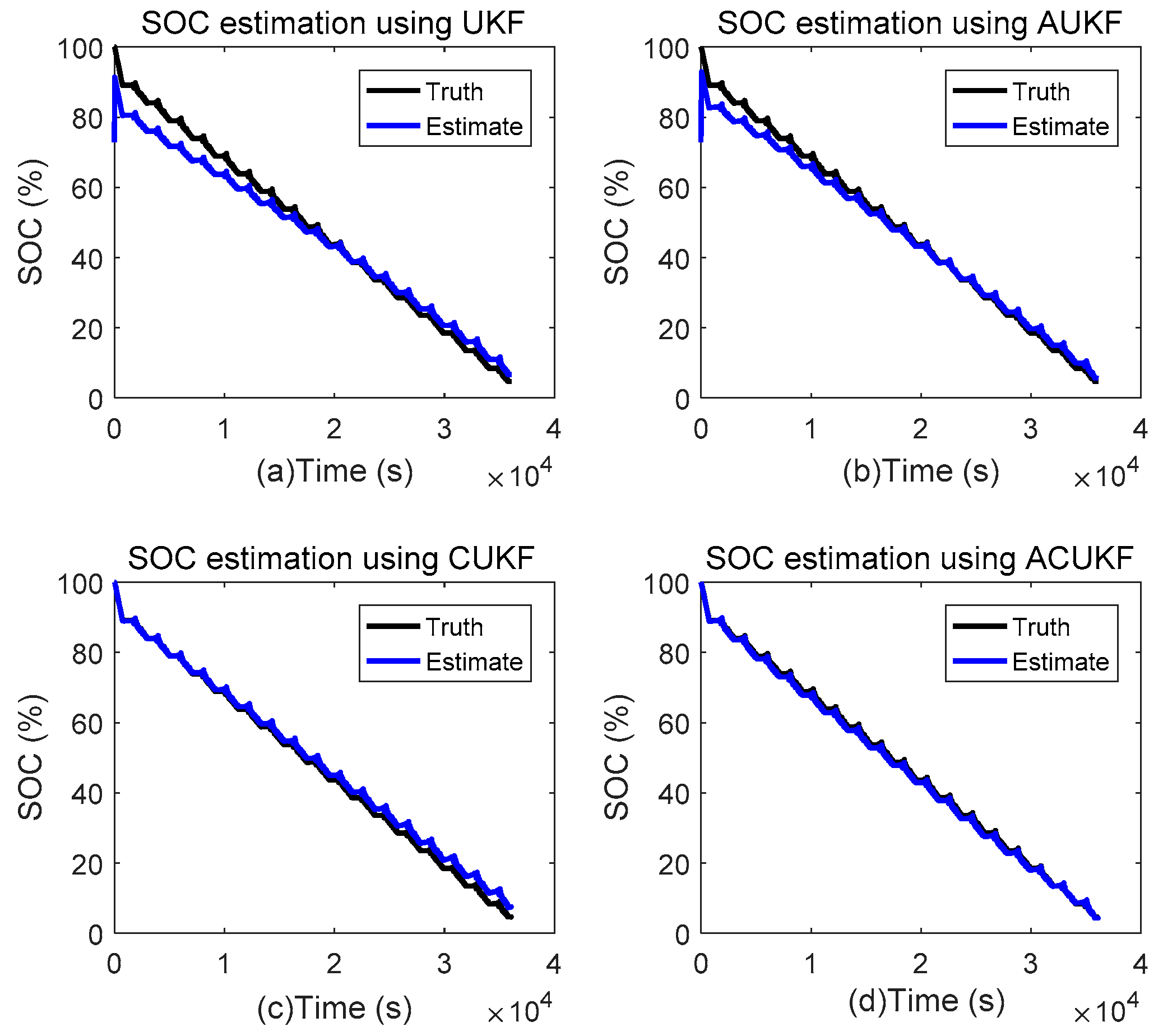
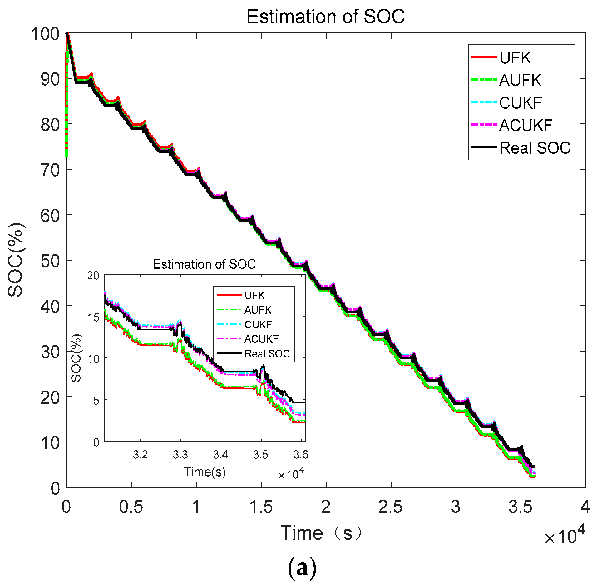
We first investigated the SOC estimation performance of the proposed method under the mixture noises mentioned above. The state variable was still initialized at 70%. The kernel width was set at 0.6 for CUKF and ACUKF. The other parameters were set in the same way as in Section 4.1. The SOC estimate results of all methods are given in Figure 9. One can see that the estimate results of UKF and AUKF at initial stage had obvious bias in this case, while CUKF and ACUKF showed excellent performance. As expected, the estimate result of the proposed ACUKF was identical with the real SOC curve according to Figure 9d. Furthermore, we can obtain the same conclusion in the SOC estimate error curves in Figure 10. From Table 3, we also know that the MSE, RMSE, and MAE results of the ACUKF approach were lower than other methods. From this result, we can conclude the following: (1) The performance of UKF and AUKF with MSE loss is influenced greatly by the impulsive point in the non-Gaussian noises. (2) The CUKF and ACUKF are robust for non-Gaussian noises environments, and they are suitable for real engineering application. (3) The ACUKF with the adaptive update of the state and measurement errors covariance matrix shows outstanding tracking ability for the SOC estimate issue.
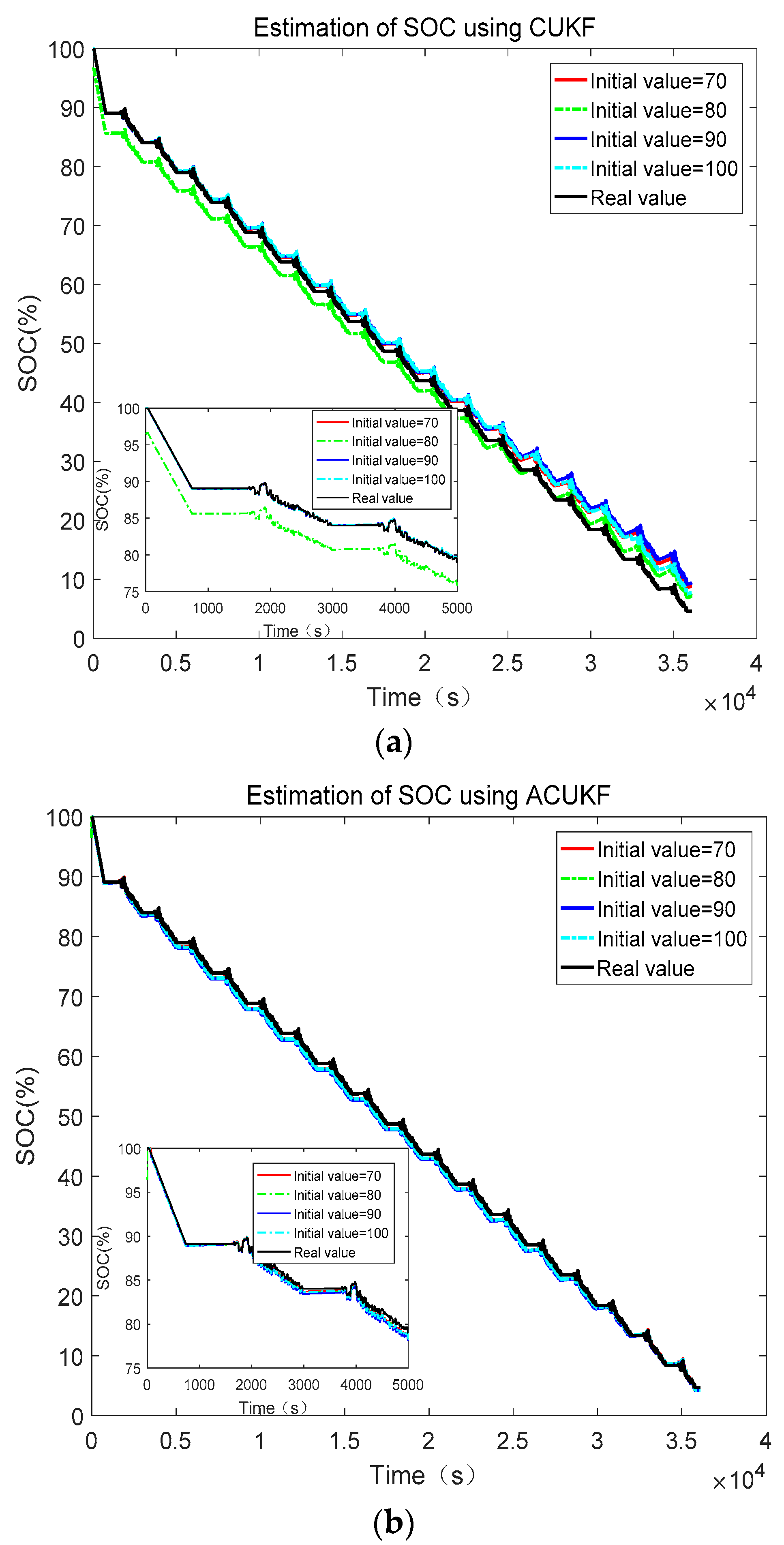
The initialization value set is an important factor for SOC estimate methods, therefore we set different initialization values to investigate the robustness of the proposed method in this experiment. Figure 11a,b show the SOC estimate results of CUKF and ACUKF under different initialization values (70%, 80%, 90%, and 100%). It is interesting that ACUKF showed better estimate results than CUKF for each initial value of state variable, which means that the adaptive covariance matrix scheme can improve the tracking ability.
Case 2: In this case, we set and by the following Gaussian mixture model as follows
where
- ,
The mixture noise, as the measurement noise generated by the model above, is shown in Figure 12.
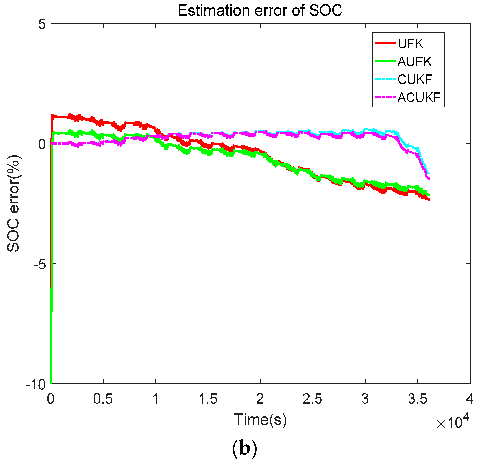
In this case, we used the SOC estimate results and error curves of all mentioned approaches to illustrate their robustness. Here, parameter settings were the same as in Case 1. The parameters were set the same as in Figure 13a,b. One can observe that the proposed CUKF- and ACUKF-based SOC estimate methods outperformed other approaches in this case. This result implies that the estimation methods based on correntropy loss are truly valid for non-Gaussian noise cases and even for the environment with many impulsive points. The MSE, RMSE, and MAE results are given in Table 4. From this result, we can come to the same conclusion. Therefore, we know that the proposed methods, i.e., CUKF and ACUKF, are appropriate selections for SOC estimate under non-Gaussian conditions. In addition, ACUKF is more effective than other model-based estimation methods.
5. Conclusions
For SOC estimate of lithium-ion battery considering the non-Gaussian noises in the system, a novel adaptive correntropy UKF method with adaptive process and measurement noises covariance was proposed in this work. Considering the statistics of system process and measurement noises with non-Gaussian characteristic in real BMS, CUKF was first employed to estimate SOC. In addition, to improve the accuracy and reliability of CUKF, we further introduced an adaptive update scheme for the process and measurement noise covariance matrices for CUKF with change in time to design adaptive CUKF for SOC estimate. Experiment results carried out on real data from the battery test system demonstrated the effectiveness and robustness of the proposed SOC method.
Author Contributions
Q.S. wrote the draft; J.Z. performed the experiment; H.Z. and W.M. were in charge of technical checking and supplied the main idea.
Acknowledgments
This work was supported by the Natural Science Basic Research Plan in Shaanxi Province of China (No. 2017JM6033), Scientific Research Program Funded by Shaanxi Provincial Education Department (No. 17JK0550), and School enterprise cooperation projects (No.103-441217024). The authors would like to thank G.L. Plett for the supplementary archives available to complement the dataset and text on BMS. Furthermore, we would like to thank the Guest Editor, assistant editor, and the reviewers for their valuable comments and suggestions, which helped us improve the quality of the manuscript.
Conflicts of Interest
The authors declare no conflict of interest.
References
- Xie, J.; Ma, J.; Bai, K. State-of-charge estimators considering temperature effect, hysteresis potential, and thermal evolution for LiFePO4 batteries. Int. J. Energy Res. 2018, 42, 2710–2727. [Google Scholar] [CrossRef]
- Zou, C.; Manzie, C.; Nesic, D. Model Predictive Control for Lithium-Ion Battery Optimal Charging. IEEE/ASME Trans. Mechatron. 2018, 23, 947–957. [Google Scholar] [CrossRef]
- Xia, B.; Chen, C.; Tian, Y.; Sun, W.; Xu, Z.; Zheng, W. A novel method for state of charge estimation of lithium-ion batteries using a nonlinear observer. J. Power Sources 2014, 270, 359–366. [Google Scholar] [CrossRef]
- Wei, Z.; Leng, F.; He, Z.; Zhang, W.; Li, K. Online state of charge and state of health estimation for a Lithium-Ion battery based on a data–model fusion method. Energies 2018, 11, 1810. [Google Scholar] [CrossRef]
- Jonghoon, K.; Cho, B.H. State-of-charge estimation and state-of-health prediction of a Li-ion degraded battery based on an EKF combined with a per-unit system. IEEE Trans. Veh. Technol. 2011, 60, 4249–4260. [Google Scholar]
- Wang, T.; Chen, S.; Ren, H. Model-based unscented Kalman filter observer design for lithium-ion battery state of charge estimation. Int. J. Energy Res. 2018, 42, 1603–1614. [Google Scholar] [CrossRef]
- Plett, G.L. Sigma-point Kalman filtering for battery management systems of LiPB-based HEV battery packs: Part 1: Introduction and state estimation. J. Power Sources 2006, 161, 1356–1368. [Google Scholar] [CrossRef]
- Plett, G.L. Sigma-point Kalman filtering for battery management systems of LiPB-based HEV battery packs: Part 2: Simulations state and parameter estimation. J. Power Sources 2006, 161, 1369–1384. [Google Scholar] [CrossRef]
- Sun, F.; Hu, X.; Zou, Y.; Li, S. Adaptive unscented Kalman filtering for state of charge estimation of a lithium-ion battery for electric vehicles. Energy 2011, 36, 3531–3540. [Google Scholar] [CrossRef]
- He, W.; Williard, N.; Chen, C.; Pecht, M. State of charge estimation for electric vehicle batteries using unscented kalman filtering. Microelectron. Reliab. 2013, 53, 840–847. [Google Scholar] [CrossRef]
- Liu, S.; Cui, N.; Zhang, C. An Adaptive Square Root Unscented Kalman Filter Approach for State of Charge Estimation of Lithium-Ion Batteries. Energies 2017, 10, 1345. [Google Scholar]
- Tian, Y.; Xia, B.; Sun, W.; Xu, Z.; Zheng, W. A modified model based state of charge estimation of power lithium-ion batteries using unscented Kalman filter. J. Power Sources 2014, 270, 619–626. [Google Scholar] [CrossRef]
- Meng, J.; Luo, G.; Gao, F. Lithium polymer battery state-of-charge estimation based on adaptive unscented Kalman filter and support vector machine. IEEE Trans. Power Electron. 2016, 31, 2226–2238. [Google Scholar] [CrossRef]
- Li, Y.; Wang, C.; Gong, J. A wavelet transform-adaptive unscented Kalman filter approach for state of charge estimation of LiFePO4 battery. Int. J. Energy Res. 2018, 42, 587–600. [Google Scholar] [CrossRef]
- Yu, Q.; Xiong, R.; Lin, C.; Shen, W.; Deng, J. Lithium-ion battery parameters and state-of-charge joint estimation based on H-infinity and unscented Kalman filters. IEEE Trans. Veh. Technol. 2017, 66, 8693–8701. [Google Scholar] [CrossRef]
- Wei, Z.; Zou, C.; Leng, F.; Soong, B.H.; Tseng, K.J. Online model identification and state-of-charge estimate for lithium-ion battery with a recursive total least squares-based observer. IEEE Trans. Ind. Electron. 2018, 65, 1336–1346. [Google Scholar] [CrossRef]
- Zhang, C.; Wang, L.; Li, X.; Chen, W.; Yin, G.G.; Jiang, J. Robust and adaptive estimation of state of charge for lithium-ion batteries. IEEE Trans. Ind. Electron. 2015, 62, 4948–4957. [Google Scholar] [CrossRef]
- Chen, X.; Shen, W.; Dai, M.; Cao, Z.; Jin, J.; Kapoor, A. Robust adaptive sliding-mode observer using RBF neural network for lithium-ion battery state of charge estimation in electric vehicles. IEEE Trans. Veh. Technol. 2016, 65, 1936–1947. [Google Scholar] [CrossRef]
- Zhao, J.; Mili, L. Robust unscented Kalman filter for power system dynamic state estimation with unknown noise statistics. IEEE Trans. Smart Grid 2017. [Google Scholar] [CrossRef]
- Liu, W.; Pokharel, P.P.; Principe, J.C. Correntropy: Properties and applications in non-Gaussian signal processing. IEEE Trans. Signal Process. 2007, 55, 5286–5298. [Google Scholar] [CrossRef]
- Ma, W.; Qu, H.; Gui, G.; Xu, L.; Zhao, J.; Chen, B. Maximum Correntropy criterion based sparse adaptive filtering algorithms for robust channel estimation under non-Gaussian environments. J. Frank. Inst. 2015, 352, 2708–2727. [Google Scholar] [CrossRef]
- Ma, W.; Chen, B.; Duan, J.; Zhao, H. Diffusion maximum Correntropy criterion algorithms for robust distributed estimation. Digit. Signal Process. 2016, 58, 10–19. [Google Scholar] [CrossRef]
- Chen, B.; Liu, X.; Zhao, H.; Principe, J.C. Maximum Correntropy Kalman filter. Automatica 2017, 76, 70–77. [Google Scholar] [CrossRef]
- Izanloo, R.; Fakoorian, S.A.; Yazdi, H.S.; Simon, D. Kalman filtering based on the maximum Correntropy criterion in the presence of non-Gaussian noise. In Proceedings of the IEEE 2016 Annual Conference on Information Science and Systems (CISS), Princeton, NJ, USA, 16–18 March 2016; pp. 500–505. [Google Scholar]
- Liu, X.; Qu, H.; Zhao, J.; Chen, B. Extended Kalman filter under maximum Correntropy criterion. In Proceedings of the 2016 International Joint Conference on Neural Networks (IJCNN), Vancouver, BC, Canada, 24–29 July 2016; pp. 1733–1737. [Google Scholar]
- Liu, X.; Chen, B.; Xu, B.; Wu, Z.; Honeine, P. Maximum Correntropy unscented filter. Int. J. Syst. Sci. 2017, 48, 1607–1615. [Google Scholar] [CrossRef]
- Wang, G.; Li, N.; Zhang, Y. Maximum Correntropy unscented Kalman and information filters for non-Gaussian measurement noise. J. Frank. Inst. 2017, 354, 8659–8677. [Google Scholar] [CrossRef]
- Liu, X.; Qu, H.; Zhao, J. Maximum Correntropy Unscented Kalman Filter for Spacecraft Relative State Estimation. Sensors 2016, 16, 1530. [Google Scholar] [CrossRef] [PubMed]
- Xin, L.; Zheng, Y.; Sun, T. A comparative study of different equivalent circuit models for estimating state-of-charge of lithium-ion batteries. Electrochim. Acta 2018, 259, 566–577. [Google Scholar]
- Zou, C.; Hu, X.; Wei, Z.; Wik, T.; Egardt, B. Electrochemical Estimation and Control for Lithium-Ion Battery Health-Aware Fast Charging. IEEE Trans. Ind. Electron. 2018, 65, 6635–6645. [Google Scholar] [CrossRef]
- He, H.; Xiong, R.; Zhang, X.; Sun, F.; Fan, J. State-of-charge estimation of the lithium-ion battery using an adaptive extended Kalman filter based on an improved Thevenin model. IEEE Trans. Veh. Technol. 2011, 60, 1461–1469. [Google Scholar]
- Raszmann, E.; Baker, K.; Shi, Y.; Christensen, D. Modeling Stationary Lithium-Ion Batteries for Optimization and Predictive Control. In Proceedings of the 2017 IEEE Power and Energy Conference at Illinois (PECI), Champaign, IL, USA, 23–24 February 2017; pp. 1–7. [Google Scholar]
- He, H.; Zhang, X.; Xiong, R.; Xu, Y.; Guo, H. Online model-based estimation of state-of-charge and open-circuit voltage of lithium-ion batteries in electric vehicles. Energy 2012, 39, 310–318. [Google Scholar] [CrossRef]
- Liu, X.; Li, W.; Zhou, A. PNGV Equivalent Circuit Model and SOC Estimation Algorithm for Lithium Battery Pack Adopted in AGV Vehicle. IEEE Access 2018, 6, 23639–23647. [Google Scholar] [CrossRef]
- Zou, C.; Hu, X.; Dey, S.; Zhang, L.; Tang, X. Nonlinear Fractional-Order Estimator with Guaranteed Robustness and Stability for Lithium-Ion Batteries. IEEE Trans. Ind. Electron. 2018, 65, 5951–5961. [Google Scholar] [CrossRef]
- Plett, G.L. Battery Management Systems, Volume II: Equivalent-Circuit Methods. Available online: http://mocha-java.uccs.edu/BMS2/ (accessed on 10 November 2018).
- Hu, C.; Youn, B.D.; Chung, J. A multiscale framework with extended kalman filter for lithium-ion battery SOC and capacity estimation. Appl. Energy 2012, 92, 694–704. [Google Scholar] [CrossRef]
- Chen, Z.; Fu, Y.; Mi, C.C. State of charge estimation of lithium-ion batteries in electric drive vehicle using extended Kalman filtering. IEEE Trans. Veh. Technol. 2013, 62, 1020–1030. [Google Scholar] [CrossRef]
- Guo, Y.F.; Zhao, Z.H.; Huang, L.M. SoC estimation of Lithium Battery Based on AEKF Algorithm. Energy Procedia 2017, 105, 4146–4152. [Google Scholar] [CrossRef]
- Daravath, S. Nonlinear Stochastic Filtering for Online State of Charge and Remaining Useful Life Estimation of Lithium-ion Battery. Master’s Thesis, South Dakota State University, Brookings, SD, USA, 2018. [Google Scholar]
- Principe, J.C. Information Theoretic Learning: Renyi’s Entropy and Kernel Perspectives; Springer: Berlin, Germany, 2010. [Google Scholar]
- Chen, B.; Xing, L.; Liang, J.; Zheng, N.; Principe, J.C. Steady-state mean-square error analysis for adaptive filtering under the maximum Correntropy criterion. IEEE Signal Process. Lett. 2014, 21, 880–884. [Google Scholar]
- Chen, B.; Principe, J.C. Maximum Correntropy estimation is a smoothed MAP estimation. IEEE Signal Process. Lett. 2012, 19, 491–494. [Google Scholar] [CrossRef]
- Partovibakhsh, M.; Liu, G. An adaptive unscented Kalman filtering approach for online estimation of model parameters and state-of-charge of lithium-ion batteries for autonomous mobile robots. IEEE Trans. Control Syst. Technol. 2015, 23, 357–363. [Google Scholar] [CrossRef]
- Ho, Z.K.; Liu, B.; Lin, Y.; Wang, W.X.; Peng, X.Q. Adaptive Square Root Unscented Kalman Filter Estimation Algorithm for Battery SOC. J. Motor Control 2014, 18, 111–116. [Google Scholar]
- Song, Q.; Song, J. An adaptive UKF algorithm for the state and parameter estimations of a mobile robot. Acta Autom. Sinica 2008, 34, 72–79. [Google Scholar] [CrossRef]
Figure 1.
Schematic diagram of the two-order resistor–capacitor (R-C) model.
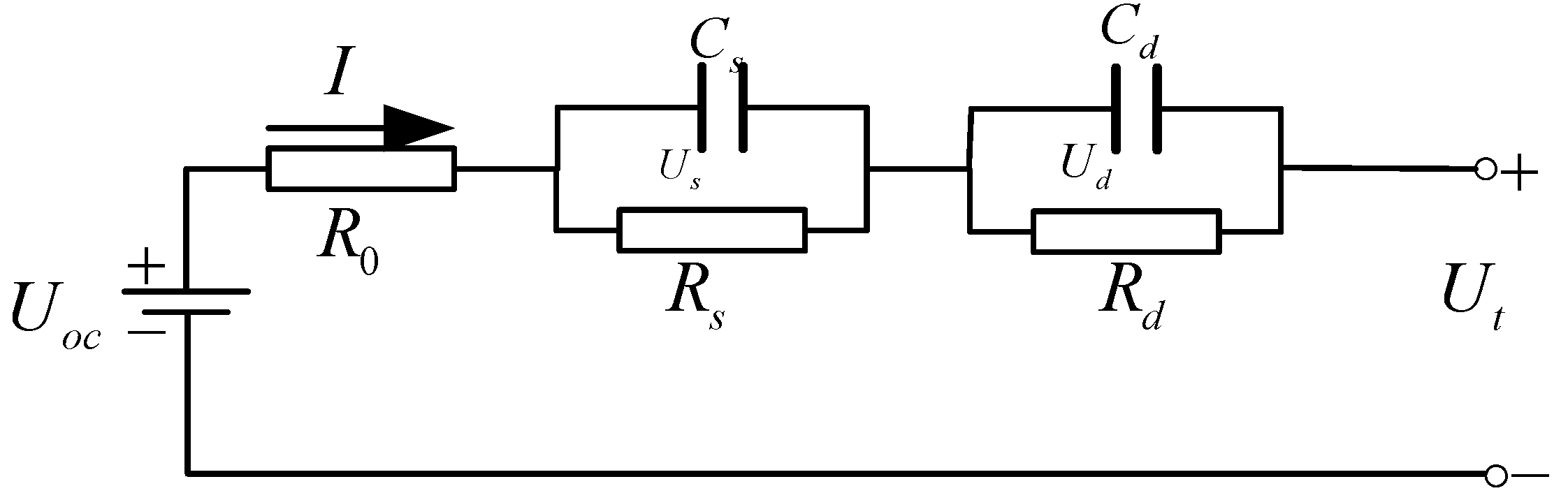
Figure 2.
Experimental and curve-fitted state of charge–open circuit voltage (SOC-OCV) correlation: (a) nonlinear relationship between SOC and OCV; (b) OCV absolute difference between real and fitting at different SOCs.
Figure 2.
Experimental and curve-fitted state of charge–open circuit voltage (SOC-OCV) correlation: (a) nonlinear relationship between SOC and OCV; (b) OCV absolute difference between real and fitting at different SOCs.
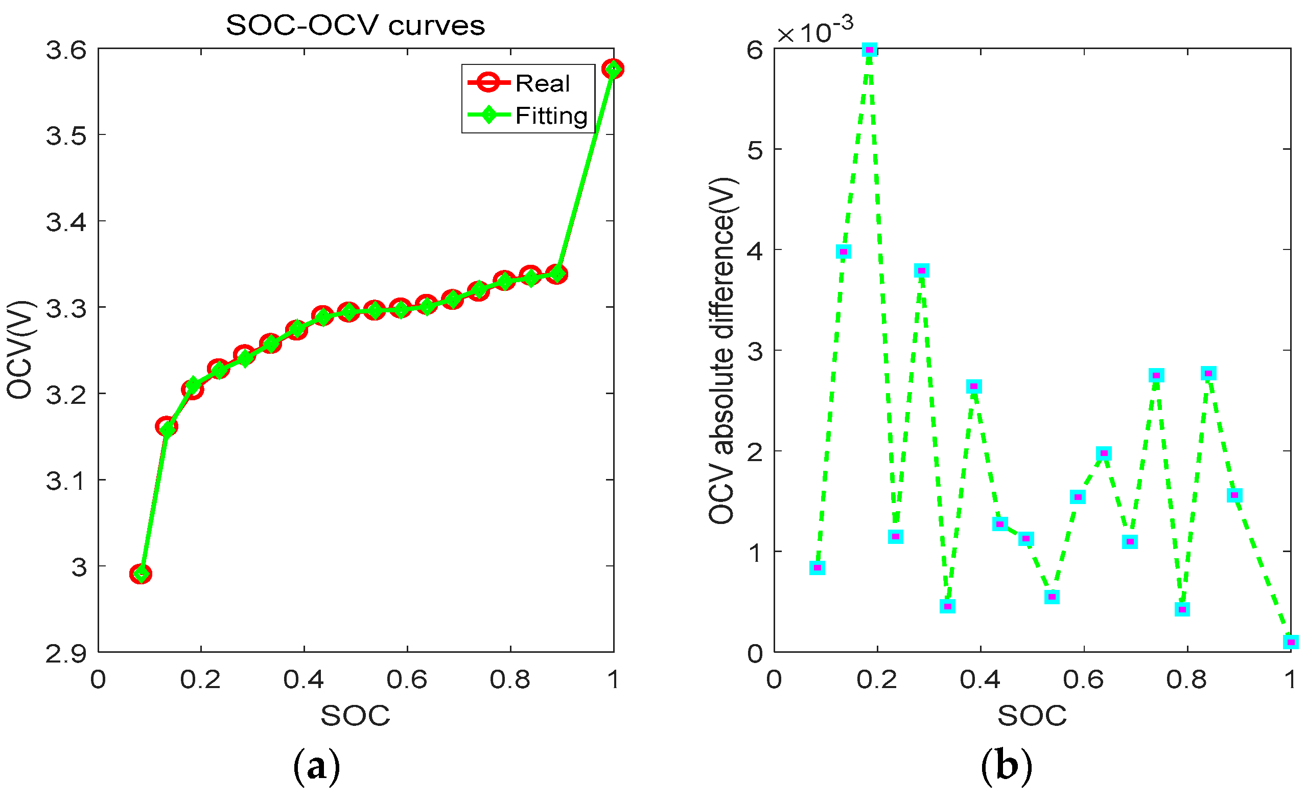
Figure 3.
Measured and calculated battery response in the hybrid pulse test: (a) current profiles; (b) voltage profiles; (c) SOC profiles.
Figure 3.
Measured and calculated battery response in the hybrid pulse test: (a) current profiles; (b) voltage profiles; (c) SOC profiles.
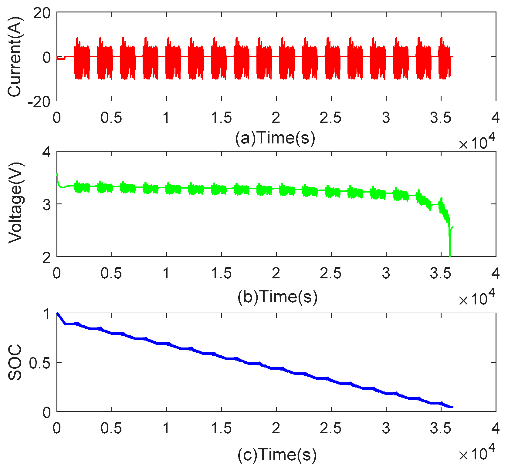
Figure 4.
Terminal voltage waveform of pulsed discharge battery.

Figure 5.
Comparisons between model output voltage and actual voltage. (a) Model output voltage and actual voltage; (b) Difference between model output voltage and actual voltage.
Figure 5.
Comparisons between model output voltage and actual voltage. (a) Model output voltage and actual voltage; (b) Difference between model output voltage and actual voltage.
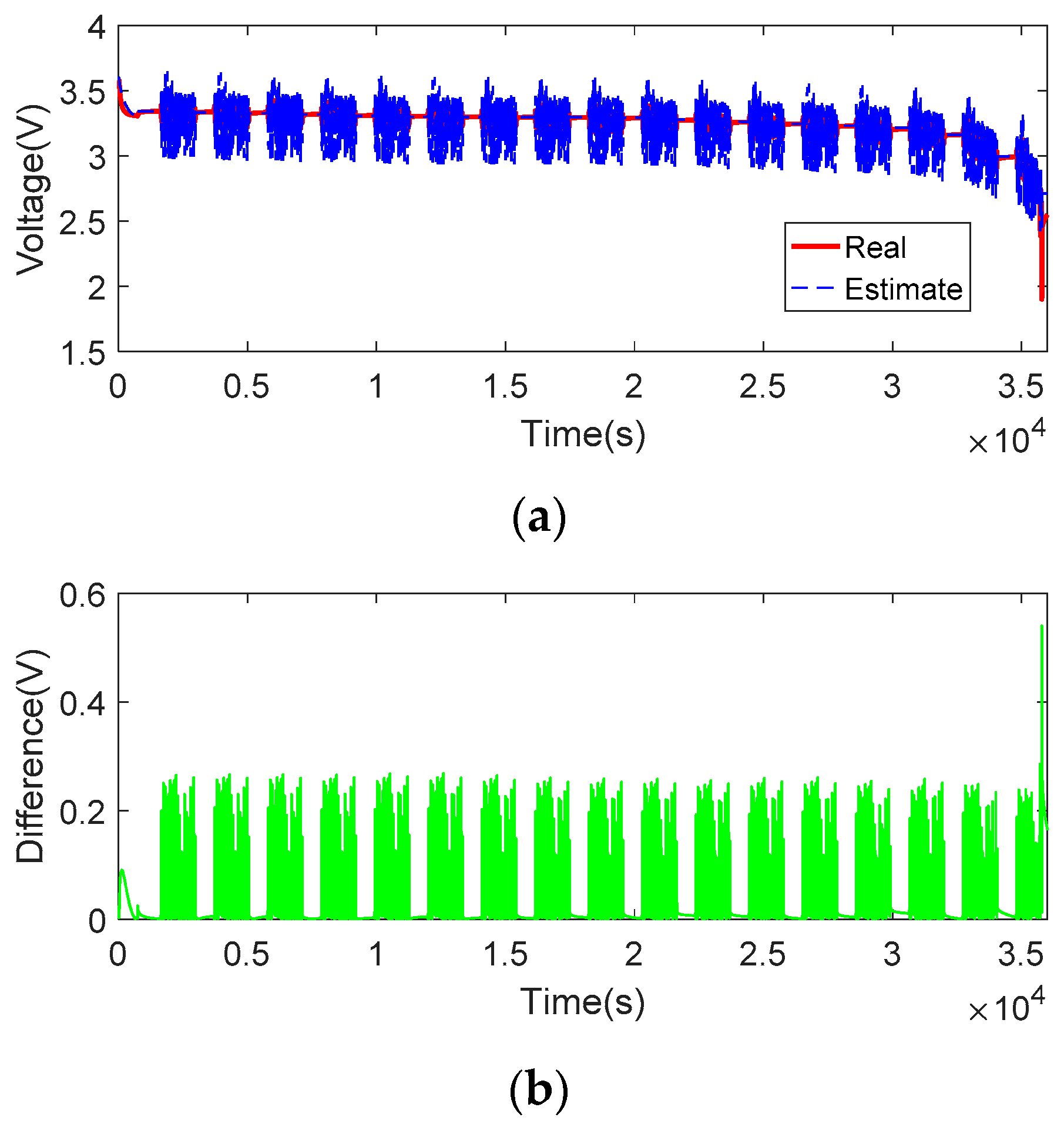
Figure 6.
SOC estimate comparison using different methods under Gaussian noises.

Figure 7.
SOC estimate errors.
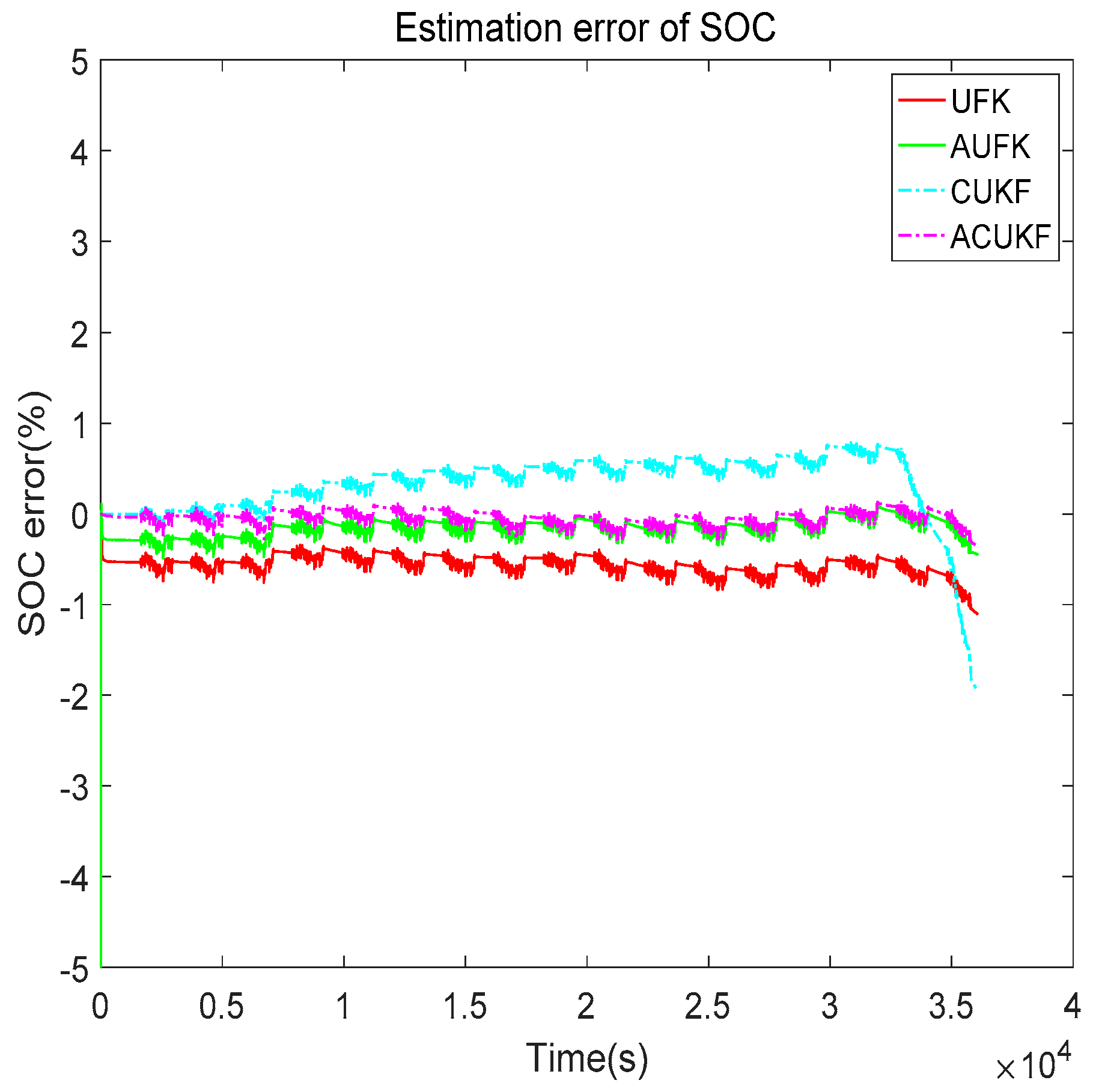
Figure 8.
Shot noise in measured output.

Figure 9.
SOC estimate comparison using different methods under shot noise. (a) SOC estimation using UKF; (b) SOC estimation using AUKF; (c) SOC estimation using CUKF; (d) SOC estimation using ACUKF.
Figure 9.
SOC estimate comparison using different methods under shot noise. (a) SOC estimation using UKF; (b) SOC estimation using AUKF; (c) SOC estimation using CUKF; (d) SOC estimation using ACUKF.

Figure 10.
SOC estimate error comparison using different methods under shot noise. (a) SOC estimate error of UKF; (b) SOC estimate error of AUKF; (c) SOC estimate error of CUKF; (d) SOC estimate error of ACUKF.
Figure 10.
SOC estimate error comparison using different methods under shot noise. (a) SOC estimate error of UKF; (b) SOC estimate error of AUKF; (c) SOC estimate error of CUKF; (d) SOC estimate error of ACUKF.
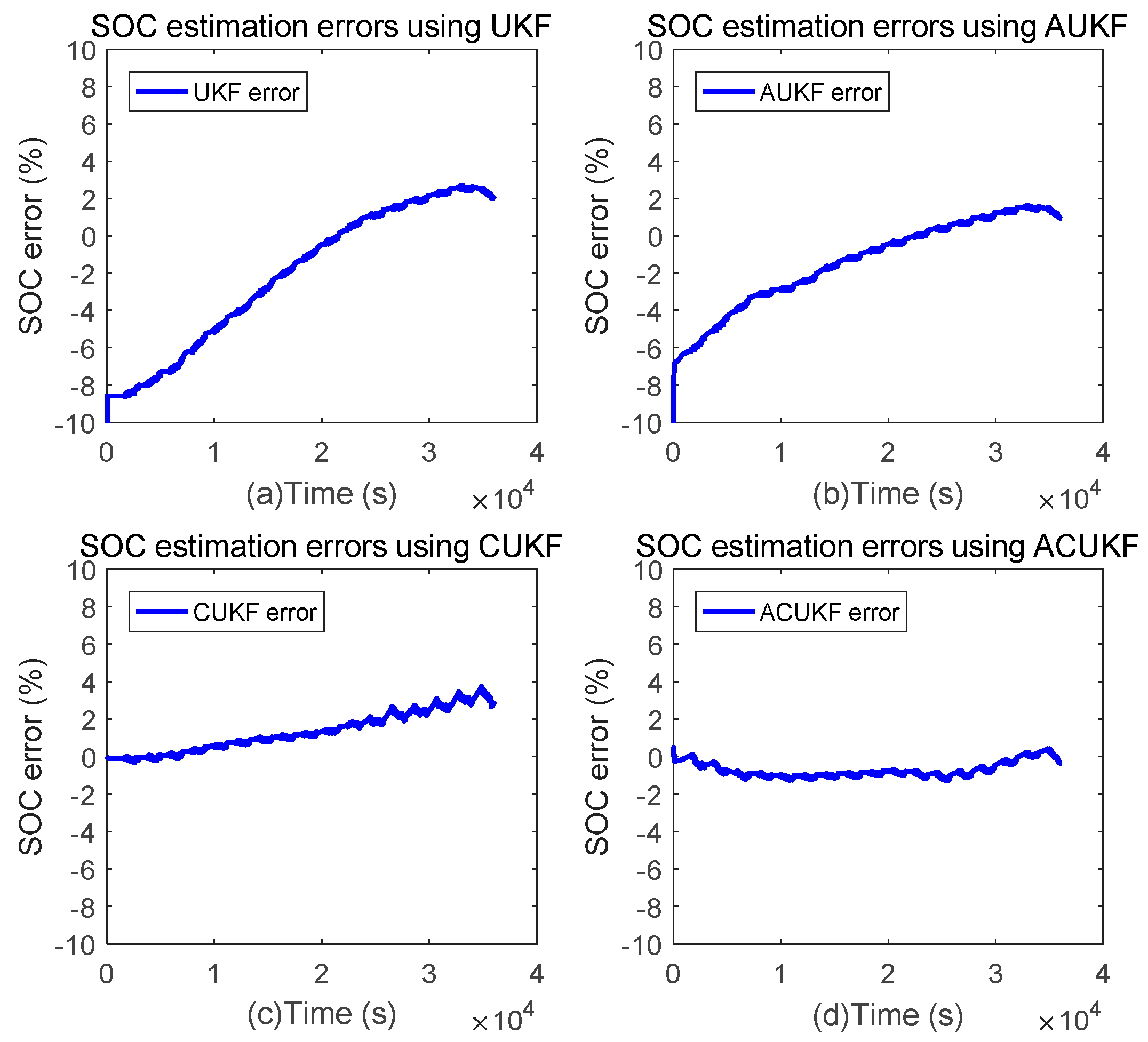
Figure 11.
SOC estimation results for correntropy unscented Kalman filter (CUKF) vs. adaptive correntropy unscented KF (ACUKF) with different SOC initialization. (a) SOC estimate results of CUKF; (b) SOC estimate results of ACUKF.
Figure 11.
SOC estimation results for correntropy unscented Kalman filter (CUKF) vs. adaptive correntropy unscented KF (ACUKF) with different SOC initialization. (a) SOC estimate results of CUKF; (b) SOC estimate results of ACUKF.

Figure 12.
Mixture noise in measured output.
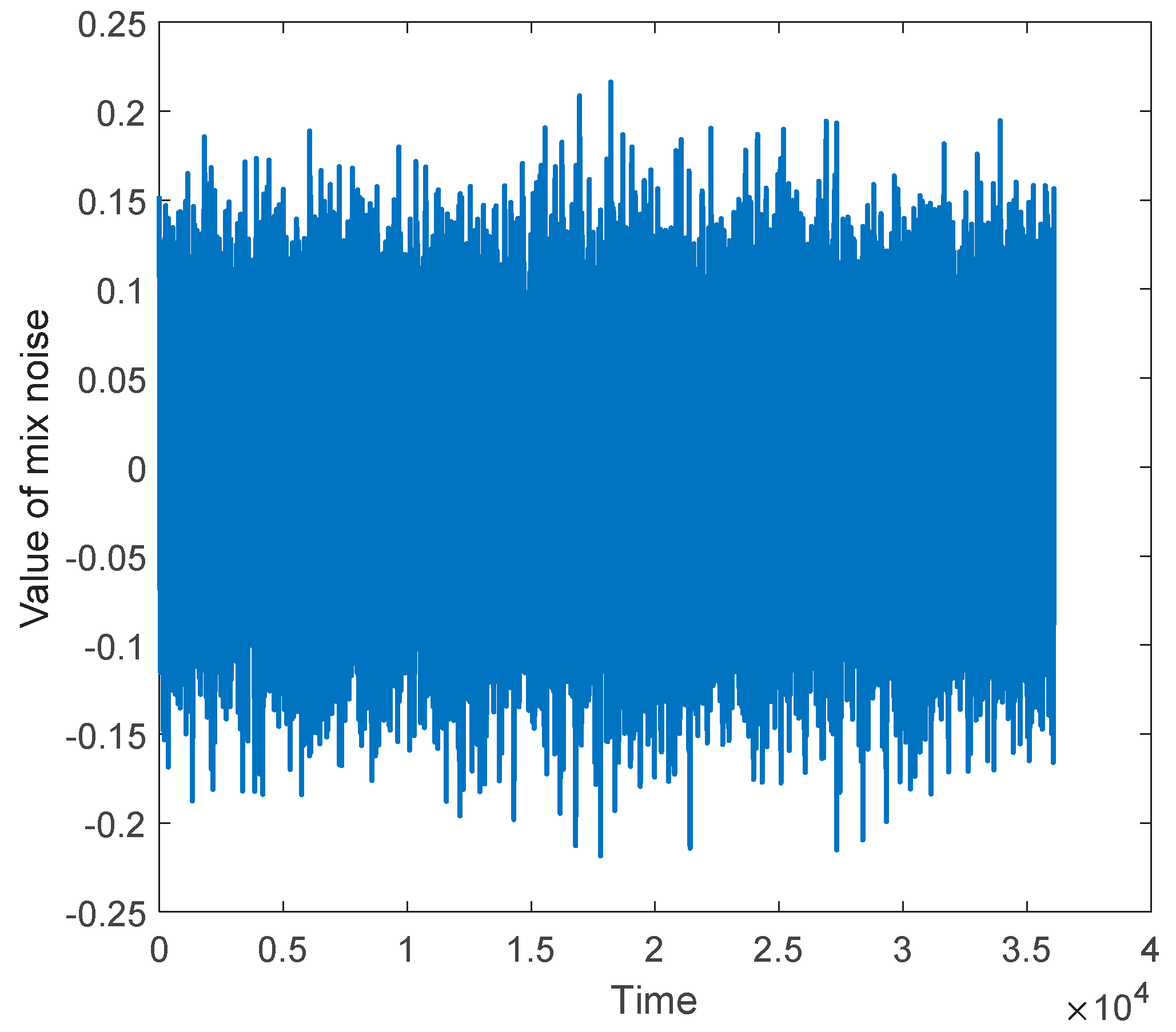
Figure 13.
SOC estimate comparison using different methods under Gaussian mixture noise: (a) SOC estimation and reference results; (b) SOC estimate errors.
Figure 13.
SOC estimate comparison using different methods under Gaussian mixture noise: (a) SOC estimation and reference results; (b) SOC estimate errors.


Table 1.
Identified parameters.
| 0.00074428 | 0.0153 | 9173.5 | 0.0050 | 28,005 |
Table 2.
Evaluation results for different SOC estimation methods.
| Algorithm | MSE (%) | RMSE (%) | MAE (%) |
|---|---|---|---|
| UKF | 0.390262 | 0.62471 | 27.1591 |
| AUKF | 0.0998027 | 0.315916 | 27.1591 |
| CUKF | 0.505981 | 0.505981 | 1.95338 |
| ACUKF | 0.0073751 | 0.0858784 | 0.36099 |
Table 3.
Evaluation results for different SOC estimation methods.
| Algorithm | MSE (%) | RMSE (%) | MAE (%) |
|---|---|---|---|
| UKF | 18.9521 | 4.3534 | 27.1591 |
| AUKF | 7.69109 | 2.77328 | 27.1591 |
| CUKF | 2.9299 | 1.7117 | 3.72793 |
| ACUKF | 0.800853 | 0.641365 | 1.2948 |
Table 4.
Evaluation results for different SOC estimation methods.
| Algorithm | MSE (%) | RMSE (%) | MAE (%) |
|---|---|---|---|
| UKF | 1.43215 | 1.19672 | 27.159 |
| AUKF | 1.38107 | 1.17519 | 27.159 |
| CUKF | 0.147968 | 0.384666 | 1.25679 |
| ACUKF | 0.132814 | 0.364437 | 1.48755 |
© 2018 by the authors. Licensee MDPI, Basel, Switzerland. This article is an open access article distributed under the terms and conditions of the Creative Commons Attribution (CC BY) license (http://creativecommons.org/licenses/by/4.0/).
Share and Cite
MDPI and ACS Style
Sun, Q.; Zhang, H.; Zhang, J.; Ma, W. Adaptive Unscented Kalman Filter with Correntropy Loss for Robust State of Charge Estimation of Lithium-Ion Battery. Energies 2018, 11, 3123. https://doi.org/10.3390/en11113123
AMA Style
Sun Q, Zhang H, Zhang J, Ma W. Adaptive Unscented Kalman Filter with Correntropy Loss for Robust State of Charge Estimation of Lithium-Ion Battery. Energies. 2018; 11(11):3123. https://doi.org/10.3390/en11113123
Chicago/Turabian StyleSun, Quan, Hong Zhang, Jianrong Zhang, and Wentao Ma. 2018. "Adaptive Unscented Kalman Filter with Correntropy Loss for Robust State of Charge Estimation of Lithium-Ion Battery" Energies 11, no. 11: 3123. https://doi.org/10.3390/en11113123
Note that from the first issue of 2016, this journal uses article numbers instead of page numbers. See further details here.