Modeling and Synchronous Optimization of Pump Turbine Governing System Using Sparse Robust Least Squares Support Vector Machine and Hybrid Backtracking Search Algorithm

Abstract

In view of the complex and changeable operating environment of pumped storage power stations and the noise and outliers in the modeling data, this study proposes a sparse robust least squares support vector machine (LSSVM) model based on the hybrid backtracking search algorithm for the model identification of a pumped turbine governing system. By introducing the maximum linearly independent set, the sparsity of the support vectors of the LSSVM model are realized, and the complexity is reduced. The robustness of the identification model to noise and outliers is enhanced using the weighted function based on improved normal distribution. In order to further improve the accuracy and generalization performance of the sparse robust LSSVM identification model, the model input variables, the kernel parameters, and the regularization parameters are optimized synchronously using a binary-real coded backtracking search algorithm. Experiments on two benchmark problems and a real-world application of a pumped turbine governing system in a pumped storage power station in China show that the proposed sparse robust LSSVM model optimized by the hybrid backtracking search algorithm can not only obtain higher identification accuracy, it also has better robustness and a higher generalization performance compared with the other existing models.

1. Introduction

With the ever-increasing electricity demand, the difference between peak load and valley load has been increasing, and the lack of peak load regulation has become a prominent problem that restricts the development of power systems [1,2]. Due to its unique functions of peak-shaving and valley-filling, and its fast response to scheduling requirements, the pumped storage power station has played an important role in balancing the power supply and demand [3,4,5]. Model identification of a pumped turbine governing system (PTGS) is of great significance for improving the control quality of the pumped storage unit (PSU) and ensuring the stable and efficient operation of the power plant [6,7]. The nonlinear system of the PSU is complex in both structure and parameters [8,9]. To achieve an accurate description of the intrinsic characteristics of the PTGS, research on model identification of the PTGS is mainly based on data-driven models such as fuzzy system [3,10,11,12], neural networks [13,14], grey system theory [15], and the Gaussian mixture model [16].

The Takagi-Sugeno (T-S) fuzzy model is an effective data-driven fuzzy modeling approach for modeling complex systems. The T–S fuzzy model has been widely applied in the model identification of the hydraulic turbine governing system (HTGS) or PTGS. Zhou et al. [3] proposed a novel data-driven T–S fuzzy model for modeling PTGS. A controlled auto-regressive (CAR) model was employed to screen the input and output variables of the identification model while the variable-length tree-seed algorithm-based competitive agglomeration algorithm was exploited to obtain the optimal clustering performance. Li et al. [10] proposed a novel T-S fuzzy model identification approach for modeling the HTGS. The novel fuzzy c-regression model clustering algorithm was employed to identify the T-S fuzzy model, and the chaotic gravitational search algorithm was proposed to optimize the parameters of the identification model. In Li et al. [11], a new fuzzy membership function was designed for hyperplane-shaped clustering to improve the effectiveness of the T-S fuzzy model identification approach. Yan et al. [12] adopted a novel improved hybrid backtracking search algorithm (IHBSA) to partition the T-S fuzzy model clustering space adaptively. By optimizing the fuzzy cluster number and the clustering centers simultaneously, the modeling accuracy can be enhanced while the complexity of the model can be reduced.

Due to its powerful nonlinear fitting and forecasting ability, the neural networks technique has been widely used in the modeling and identification of various nonlinear systems [13,17]. The main process of the model identification of a hydroelectric generating unit or PSU based on neural networks is optimizing the weights and biases of each neuron in the network with the help of training algorithms such as back-propagation, gradient descent, and intelligent optimization algorithms, and then, the nonlinear characteristics of HTGS or PTGS can be effectively described using the identification model. In Kishor et al. [13], the neural networks nonlinear autoregressive network with exogenous signal (NNARX) model and the adaptive network-based fuzzy inference system (ANFIS) were applied to simulate the hydropower plant model at random load disturbances. The ANFIS model turned out to perform better than the NNARX model in identifying the turbine/generator speed. Kishor and Singh [14] investigated the performance of the NNARX model in the model identification of elastic and inelastic hydropower plants.

The training process of the fuzzy and neural network models is mainly based on empirical risk minimization criterion, which makes these models suffer from problems of instability and local extremum. Thus, it is necessary to introduce the least squares support vector machine (LSSVM), which is based on structural risk minimization criterion. The learning process of LSSVM can balance the empirical risk and confidence range. It overcomes the instability and local extremum problems of neural network models.

The research works on model identification of the PTGS include most of the fuzzy system models and the neural networks models, and have many achievements. However, most of the current studies on model identification of the PTGS or HTGS do not consider the effects of noise and outliers, the robustness and generalization ability of the identification model are seriously affected. Taking the neural network identification model as an example, the training process of it takes the error quadratic loss function as the objective function, and the model stability and robustness are highly susceptible to noise and outliers. Therefore, it is necessary to further study the strategies to improve the robustness and stability of the identification model. The robust modeling method can give a smaller weight to the data points that have been identified as noise and outliers and inhibit their impact on modeling through sample weighting and robust learning [18]. The robustness of identification models can then be improved. The robust modeling method has been widely applied in pattern recognition [19], metallurgy [20], and other industrial fields.

For nonlinear system modeling, one of the primary problems is to determine the model structure, that is, the input variables selected in the identification process. An ideal combination of input variables should be a set of suitable numbers that can also describe the nonlinear characteristics of the system adequately. Zhou et al. [3] introduced an economical parameter CAR model to select the input and output formats of the T-S fuzzy model. Zhang et al. [21] proposed a hybrid backtracking search algorithm (HBSA) algorithm, of which the real-valued backtracking search algorithm (BSA) is exploited to optimize the biases and weights of the nonlinear model, and the binary-valued BSA is used to select the most suitable input variables. Yan et al. [12] proposed an IHBSA algorithm to partition the fuzzy space and identify the premise parameters of the T-S fuzzy model simultaneously.

This study proposes a sparse robust LSSVM (S-R-LSSVM) model for the model identification of the PTGS. The maximum linearly independent set is introduced to improve the sparsity of the support vectors and reduce the complexity of the identification model. The improved normal distribution weighted function is introduced to enhance the robustness of the model to noise and outliers. To further improve the accuracy and generalization performance of the identification model, the design idea of synchronous optimization for the model structure and parameters is introduced. A binary-real coded HBSA algorithm is proposed to optimize the input variables, the kernel, and the regularization parameters synchronously. To verify the effectiveness of the proposed S-R-LSSVM identification model optimized by the HBSA algorithm (HBSA-S-R-LSSVM) and apply it in engineering application, the proposed model is tested using three nonlinear systems with noises and outliers. The first two nonlinear systems are the SinC mathematical function and a nonlinear differential equation, respectively. The third application is to the PSU.

The rest of the paper is organized as follows. Section 2 gives a brief introduction to the S-R-LSSVM model. Section 3 presents how synchronous optimization for the S-R-LSSVM identification model is realized using HBSA. Section 4 gives two benchmark models, including a SinC mathematical function and a nonlinear differential equation to identify the effectiveness of the S-R-LSSVM identification model. In Section 5, the robust modeling and synchronous optimization of the PTGS is realized by applying the HBSA-S-R-LSSVM model in a pumped storage power station in China. Lastly, Section 6 draws the conclusions of this study.

2. Sparse Robust Least Squares Support Vector Machine

2.1. Least Squares Support Vector Machine

Considering a training set $\left\{\left(x_i,y_i\right),i=1,2,\dots ,N\right\}$, where $x_i\in R^n$ denotes the input data and $y_i\in R$ denotes the output data. The purpose of the LSSVM model is to establish a linear regression equation of the input vectors and the output vector [22]:

$$y_i=w^T\varphi \left(x_i\right)+b$$

(1)

where N denotes the number of training samples; w denotes the unit normal vector of the hyperplane; b denotes the distance from the origin to the hyperplane; and $\varphi (\cdot )$ denotes the nonlinear mapping function.

The linear regression equation is then transformed into an optimization problem according to the structural risk minimization criteria:

$$\begin{array}{l}\mathrm{Min}\frac{1}{2}{\Vert w\Vert }^2+\frac{1}{2}\gamma {\displaystyle \sum _{i=1}^N{{\epsilon }_i}^2}\\ \mathrm{subject}\mathrm{to}\{\begin{array}{l}{y}_i=\left(w^T\varphi \left(x_i\right)+b\right)+{\epsilon }_i\\ {\epsilon }_i\ge 0\end{array}\end{array}$$

(2)

where ε_i is the fitting error of the i-th training sample, and γ is the regularization parameter.

The above optimization problem is converted into its dual form and then solved according to the Lagrange multiplier method. The dual form is as follows:

$$L\left(w,b,\epsilon ,a\right)=\frac{1}{2}{w}^{T}w+\frac{1}{2}\gamma {\displaystyle \sum _{i=1}^N{{\epsilon }_i}^2}-{\displaystyle \sum _{i=1}^N{a}_i\left(w^T\varphi \left(x_i\right)+b+{\epsilon }_i-y_i\right)}$$

(3)

where a_i,i = 1,2,…,N represent the Lagrange multipliers.

According to the Karush-Kuhn-Tucker (KKT) condition, the first derivatives of L are calculated:

$$\{\begin{array}{l}\frac{\partial L}{\partial w}=w-{\displaystyle \sum _{i=1}^N{a}_i\varphi \left(x_i\right)}=0\\ \frac{\partial L}{\partial b}={\displaystyle \sum _{i=1}^N{a}_i}=0\\ \frac{\partial L}{\partial {\epsilon }_i}=\gamma {\epsilon }_i-a_i=0\\ \frac{\partial L}{\partial a_i}=w^T\varphi \left(x_i\right)+b+{\epsilon }_i-y_i=0\end{array}$$

(4)

According to Equation (4), the following equations are obtained:

$$\{\begin{array}{l}w={\displaystyle \sum _{i=1}^N{a}_i\varphi \left(x_i\right)}\\ {\displaystyle \sum _{i=1}^N{a}_i}=0\\ \gamma {\epsilon }_i=a_i\\ w^T\varphi \left(x_i\right)+b+{\epsilon }_i=y_i\end{array}$$

(5)

Equation (5) can be described in its matrix representation:

$$\left[\begin{array}{cccc}I& 0& 0& -G\\ 0& 0& 0& -Y^T\\ 0& 0& \gamma I& -I\\ G& Y& I& 0\end{array}\right]\left[\begin{array}{c}w\\ b\\ \epsilon \\ a\end{array}\right]=\left[\begin{array}{c}0\\ 0\\ 0\\ y\end{array}\right]$$

(6)

Equation (6) can be transferred into:

$$\left[\begin{array}{cc}0& Y^T\\ Y& G{G}^T+{\gamma }^{-1}I\end{array}\right]\left[\begin{array}{c}b\\ a\end{array}\right]=\left[\begin{array}{c}0\\ y\end{array}\right]$$

(7)

where $Y={\left[1,1,\dots ,1\right]}^T$ represents the N-dimensional unit vector; $\epsilon =\left[{\epsilon }_1,{\epsilon }_2,\dots ,{\epsilon }_N\right]$; $y={\left[y_1,y_2,\dots ,y_N\right]}^T$ represents the output vector; $a={\left[a_1,a_2,\dots ,a_N\right]}^T$ and b are the parameters of the LSSVM model; and $G={\left[\varphi \left(x_1\right),\varphi \left(x_2\right),\dots ,\varphi \left(x_N\right)\right]}^T,G{G}^T=K\left(x_i,x_j\right)$ is the kernel function of the LSSVM model.

The values of $a={\left[a_1,a_2,\dots ,a_N\right]}^T$ and b can be obtained according to the least square method, and the LSSVM regression model can be obtained:

$$f\left(x\right)={\displaystyle \sum _{i=1}^N{a}_{i}K\left(x_i,x\right)+b}$$

(8)

In this study, the Gaussian kernel function was selected as the kernel function of the LSSVM model:

$$K\left(u,v\right)=\exp \left(-\frac{{\Vert u-v\Vert }^2}{{\sigma }^2}\right)$$

(9)

where $\sigma \in R$ denotes the kernel parameter of the Gaussian kernel function.

2.2. Sparse Robust Least Squares Support Vector Machine

An S-R-LSSVM model was proposed in this section. The sparse solution for LSSVM was realized by introducing the maximum linearly independent set, while the robustness of the model was improved by introducing the robust weighted function.

2.2.1. Sparse Solution for LSSVM Based on Maximum Linearly Independent Set

(1) Maximum linearly independent set

The mapping of the sample vector $x_i$ in the feature space to the hyperplane can be represented as $\varphi \left(x_i\right)$. The mapping of all of the sample vectors $\left\{x_1,x_2,\dots ,x_i,\dots ,x_N\right\}$ in the feature space to the hyperplane constitutes a mapping matrix $A=\left\{\varphi \left(x_1\right),\varphi \left(x_2\right),\dots ,\varphi \left(x_i\right),\dots ,\varphi \left(x_N\right)\right\}$. The basis of the mapping matrix in the hyperplane $\left\{\varphi \left({\tilde{x}}_1\right),\varphi \left({\tilde{x}}_2\right),\dots ,\varphi \left({\tilde{x}}_s\right)\right\}$ is linearly independent, and any vector $\varphi \left(x_i\right)$ in the hyperplane can be described as a linear combination of the basis. As can be seen in Equation (10), the mapping matrix in the hyperplane can be expressed as the linear combination of its basis:

$$\left[\begin{array}{c}\varphi \left(x_1\right)\\ \varphi \left(x_2\right)\\ ⋮\\ \varphi \left(x_N\right)\end{array}\right]=\left[\begin{array}{cccc}{a}_{11}& a_{12}& \cdots & a_{1s}\\ a_{21}& a_{22}& \cdots & a_{2s}\\ ⋮& ⋮& ⋮& ⋮\\ a_{N1}& a_{N2}& \cdots & a_{Ns}\end{array}\right]\left[\begin{array}{c}\varphi \left({\tilde{x}}_1\right)\\ \varphi \left({\tilde{x}}_2\right)\\ ⋮\\ \varphi \left({\tilde{x}}_s\right)\end{array}\right]$$

(10)

From the above description, it can be seen that the mapping of the sample vectors can be replaced by the basis of the mapping matrix to improve the sparseness of the solution and reduce the model complexity of the LSSVM model. In this study, the matrix-algebraic theory is employed to obtain the maximum linearly independent set to improve the sparseness of the LSSVM model [23,24,25].

(2) Sparse solution for LSSVM

According to linear algebra theory, if $\left\{\varphi \left(x_1\right),\varphi \left(x_2\right),\dots ,\varphi \left(x_i\right),\dots ,\varphi \left(x_N\right)\right\}$ is linearly related, there is at least one $\varphi \left(x_q\right)$ such that $\varphi \left(x_q\right)={\displaystyle \sum _{i=1,i\ne q}^N{\lambda }_i}\varphi \left(x_i\right)$, where ${\lambda }_i\in R$ and ${\lambda }_i$ are not all zero. Then, the kernel function of LSSVM model can be written as:

$$K\left(x_q,x_q\right)=\varphi \left(x_q\right)\varphi \left(x_q\right)={\displaystyle \sum _{i=1,i\ne q}^N{\displaystyle \sum _{j=1,j\ne q}^N{\lambda }_i}}{\lambda }_{j}K\left(x_i,x_j\right)$$

(11)

The maximum linearly independent set of $\left\{\varphi \left(x_1\right),\varphi \left(x_2\right),\dots ,\varphi \left(x_i\right),\dots ,\varphi \left(x_N\right)\right\}$ can be obtained in the following steps:

Step 1: Initialize the maximum linearly independent set as $B=\left\{\varphi \left(x_1\right)\right\}$, and set up an empty set $C=\varnothing$;

Step 2: For $\varphi \left(x_k\right),k=2,3,\dots ,N$, obtain the minimum $f\left(\lambda \right)$ according to the Lagrange multiplier method:

$$\min f\left(\lambda \right)=\min {\left[\varphi \left(x_k\right)-{\displaystyle \sum _{\varphi \left(x_k\right)\in C}{\lambda }_i\varphi \left(x_i\right)}\right]}^T\left[\varphi \left(x_k\right)-{\displaystyle \sum _{\varphi \left(x_k\right)\in C}{\lambda }_i\varphi \left(x_i\right)}\right]$$

(12)

Step 3: If the minimum value of f(λ) is zero, it means that ϕ(x_k) can be represented by the linear combination of the vectors in B. Then, ϕ(x_k) is discarded and added to C; otherwise, ϕ(x_k) can be added to set B;

Step 4: Return to step 2, traverse all $\varphi \left(x_k\right),k=2,3,\dots ,N$ until the number of vectors in B can no longer increase. The final linear independent set B and set C are obtained, and B is the maximum linearly independent set of $\varphi \left(x_1\right),\varphi \left(x_2\right),\dots ,\varphi \left(x_i\right),\dots ,\varphi \left(x_N\right)$. Any vector in matrix A can be represented as a linear combination of the vectors in B.

The sample vectors in the feature space corresponding to the maximum linearly independent set B constitute a sparse training sample set $\{(x_i,y_i),i=1,2,\dots ,K\}$, where K denotes the size of the sparse training sample set.

2.2.2. Robust Weighted Function Based on Improved Normal Distribution

Since the loss function of the common LSSVM is the sum of the squared errors and the regularization parameter γ remains unchanged throughout the training process, the robustness of the objective function is insufficient, and it is easily interfered by noise and outliers. The common LSSVM model tends to be more sensitive to data points with greater errors to obtain the minimum fitness value, which will increase the negative impact of the abnormal samples on the objective function. To get rid of this drawback of the common LSSVM model, Suykens et al. proposed a weighted LSSVM (WLSSVM) by adding a weighted coefficient to the quadratic term of the objective function of the common LSSVM model [18]. The mathematical expression of optimization problem for the WLSSVM model is as follows:

$$\begin{array}{l}\mathrm{Min}\frac{1}{2}{\Vert w\Vert }^2+\frac{1}{2}\gamma {\displaystyle \sum _{i=1}^K{v}_i{{\epsilon }_i}^2}\\ s.t.\{\begin{array}{l}{y}_i=w^T\varphi \left(x_i\right)+b+{\epsilon }_i\\ {\epsilon }_i\ge 0,i=1,\dots ,K\end{array}\end{array}$$

(13)

The following equation is obtained according to the Lagrange multiplier method:

$$L\left(w,b,\epsilon ,a\right)=\frac{1}{2}{w}^{T}w+\frac{1}{2}\gamma {\displaystyle \sum _{i=1}^K{v}_i{{\epsilon }_i}^2}-{\displaystyle \sum _{i=1}^K{a}_i\left(w^T\varphi \left(x_i\right)+b+{\epsilon }_i-y_i\right)}$$

(14)

where $\left\{a_i\right\},i=1,2,\dots ,K$ denotes the Lagrange multipliers, and $\left\{v_i\right\},i=1,2,\dots ,K$ is a weighting factor.

To obtain the value of $a_i$ and b, the following equation is first obtained according to the KKT condition:

$$\left[\begin{array}{cccc}0& 1& \cdots & 1\\ 1& K\left(x_1,x_1\right)+\frac{1}{\gamma v_1}& \cdots & K\left(x_1,x_K\right)\\ ⋮& ⋮& \ddots & ⋮\\ 1& K\left(x_K,x_1\right)& \cdots & K\left(x_K,x_K\right)+\frac{1}{\gamma v_K}\end{array}\right]\left[\begin{array}{c}b\\ a_1\\ ⋮\\ a_K\end{array}\right]=\left[\begin{array}{c}0\\ y_1\\ ⋮\\ y_K\end{array}\right]$$

(15)

where the weighting factor $\left\{v_i\right\},i=1,2,\dots ,K$ is usually determined according to the weighting function proposed by Suykens [18]:

$$v_i=\{\begin{array}{ll}1,& \left|{\epsilon }_i/\widehat{s}\right|\le c_1\\ \frac{c_2-\left|{\epsilon }_i/\widehat{s}\right|}{c_2-c_1},& c_1\le \left|{\epsilon }_i/\widehat{s}\right|\le c_2\\ {10}^{-4},& otherwise\end{array}$$

(16)

where $\widehat{s}=1.483MAD\left({\zeta }_i\right)$ is the robustness estimation of the standard deviation of the error; c₁ and c₂ are constant, where c₁ = 2.5, c₂ = 3 [18].

In Equation (16), the error item is assumed to obey the Gauss distribution. The weighting factor is calculated according to the degree to which the error deviates from the mean standard deviation. However, the noise and outliers in actual industrial application may not obey the Gauss distribution, which limits the application of the weighting function [26,27,28]. In addition, in the modeling process of a complex nonlinear system, the effective information for modeling usually appears at the turning points of the working condition. Stationary data in steady condition, in the other way, contains less information. The modeling error of the turning points is usually between that of the stationary data and the outlier data, which requires the weighting function focus on the samples of intermediate error, and weakens the influence of the outliers and the redundant stable data. This study introduces the weighting function based on improved normal distribution [29] to balance the weight of the turning points, the stationary data, and the noise and outliers in the modeling process. The weighting function based on improved normal distribution is expressed as follows:

$$v_i=\{\begin{array}{ll}\exp \left(\frac{{\left(\left|{\epsilon }_i\right|-\mu \right)}^2}{u_1{s}^2}\right)& \left|{\epsilon }_i\right|<\mu \\ \exp \left(\frac{{\left(\left|{\epsilon }_i\right|-\mu \right)}^2}{u_2{s}^2}\right)& \left|{\epsilon }_i\right|\ge \mu \end{array}$$

(17)

where $\mu$ represents the mean of $\left|{\epsilon }_i\right|$; and $s$ represents the standard deviation of $\left|{\epsilon }_i\right|$. $\mu$ and $s$ can be calculated as follows:

$$\mu =\frac{1}{K}{\displaystyle \sum _{i=1}^K\left|{\epsilon }_i\right|}$$

(18)

$$S=\sqrt{\frac{1}{K}{\displaystyle \sum _{i=1}^K{\left(\left|{\epsilon }_i\right|-\mu \right)}^2}}$$

(19)

According to the weighting function based on improved normal distribution, the sample in which the modeling error is in the middle of the probability density curve of the normal distribution will be given a greater weight, while the sample in which the modeling error is at the end of the probability density curve will be given a smaller weight. Two width adjustment parameters, u₁ = 9.7 and u₂ = 7.6, are introduced to balance the symmetry characteristics of a normal distribution [29,30]. In this way, the robust LSSVM model based on the weighting function using the improved normal distribution is insensitive to the error caused by noise and outliers, and can reduce the weight of the stationary data.

3. Model Identification of PTGS Based on HBSA-S-R-LSSVM

Model identification of the PTGS refers to the modeling and identification of the input and output characteristics of the PSU through methods with strong approximation and fitting capabilities such as neural networks, fuzzy system, and LSSVM. The S-R-LSSVM model is employed to describe the PTGS in this study. In the model identification process, model structure determination and model parameters optimization are two important procedures. The traditional method for model identification of the PTGS is to first determine the model structure, namely model input variables, through experiential selection, trial-and-error, or hypothesis testing, and then search for the optimal parameters using grid search or intelligent optimization algorithms. However, the traditional methods for model identification fail to consider the interaction between input variables selection and model parameters optimization, which makes it difficult to obtain the optimal model structure and model parameters synchronously. In this study, a model identification strategy for the synchronous optimization of the model structure and parameters is proposed. The model structure and parameters of the S-R-LSSVM model are optimized synchronously using a hybrid backtracking search algorithm.

3.1. Synchronous Optimization Design for the S-R-LSSVM Identification Model

For a complex time-varying nonlinear system such as the PTGS, the nonlinear auto regressive with exogenous inputs (NARX) model is usually employed to describe the nonlinear relationship between the inputs and outputs:

$$y(k)=f[y(k-1),y(k-2),\dots ,y(k-m),u(k-1),u(k-2),\dots ,u(k-n)]$$

(20)

where f(·) represents the S-R-LSSVM model described in the previous section; y(k−m) represents the history output of the system; u(k−n) represents the history control input of the system; and m and n represent the output delay and the control input delay of the system, respectively.

To describe the PTGS system accurately using the above NARX model, one of the most important things is to determine the input variables. Too many input variables may cause information redundancy and increase the computation burden, and thus affect the efficiency and accuracy of the identification model. A lack of input variables, in the other way, may lead to insufficient capturing of the dynamic characteristics of the identification model, resulting in the underfitting of the model. An ideal combination of input variables should be a set of suitable numbers that can also describe the nonlinear characteristics of the system adequately. What’s more, the regularization parameter γ and the kernel parameter σ of the S-R-LSSVM model play an important role in the simulation accuracy and generalization performance of the model. To obtain the optimal model structure and parameters, this study proposes a hybrid optimization strategy to optimize the model structure and parameters synchronously. The hybrid optimization problem is translated into a binary and real-coded multidimensional parameter optimization problem, where the binary-coded strategy is employed to select the optimal input variables, while the real-coded strategy is selected to optimize the model parameters.

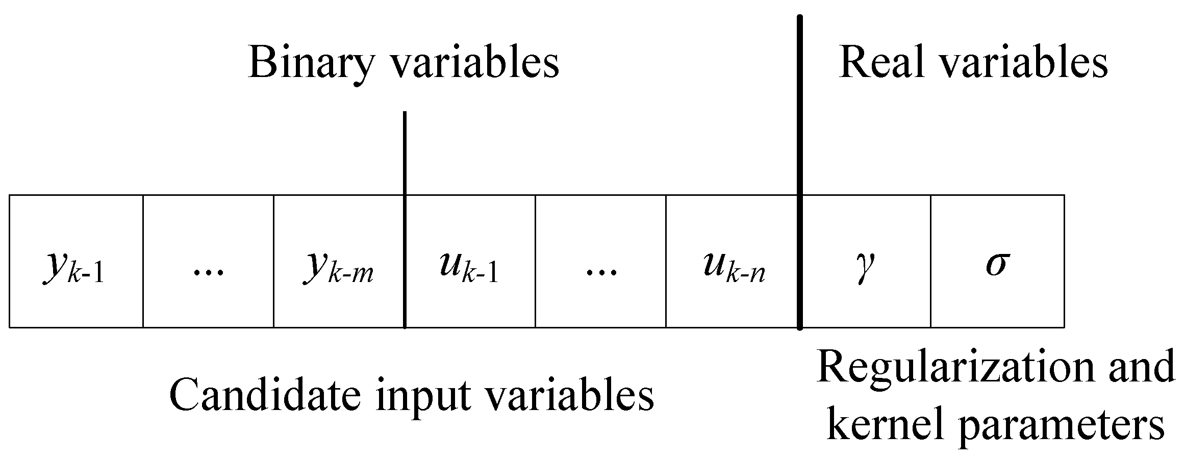
The inputs’ selection in the model identification process is an optimization problem of discrete variables. Combined with actual engineering application, n historical control inputs and m history outputs of the system are predefined as candidate input variables. The n + m candidate input variables are than coded as a binary variable. Each element of the binary variable corresponds to a candidate input variable. When the value of corresponding element is 0, the candidate input variable is discarded; otherwise, the candidate input variable is retained as the input of the model. The regularization parameter and kernel parameter of S-R-LSSVM are coded into a real variable with a length of 2. The dimension of the hybrid variable is then n + m + 2. The optimal model inputs, the best kernel, and the regularization parameters can be obtained synchronously using an algorithm with the ability to optimize the binary and real variables at the same time.

3.2. Real-Coded the Backtracking Search Algorithm

The backtracking search algorithm (BSA) proposed by Civicioglu is a stochastic optimization algorithm based on the evolutionary framework [31]. Since the BSA algorithm contains only one control parameter and is insensitive to the initial value, it can solve different optimization problems effectively. What’s more, the BSA algorithm can generate a memory to store a randomly selected historical population and then use it to generate a search direction matrix. The basic principle of the BSA can be described in five steps: initialization, selection-I, mutation, crossover, and selection-II [21,31]. The traditional BSA algorithm belongs to a real-coded optimization algorithm and is recorded as real-coded BSA (RBSA). To solve discrete optimization problems in scientific research and engineering applications, it is necessary to modify the coding mechanism of the RBSA. Since the inputs’ selection problem in the model identification process is actually an optimization problem of discrete variables, it is necessary to convert the real-coded BSA algorithm into a binary-coded BSA algorithm.

3.3. Binary-Coded Backtracking Search Algorithm

To solve discrete optimization problems, Ahmed et al. [32] proposed a binary version of BSA, called binary-coded BBSA (BBSA). The selection, mutation, and crossover operators of the BBSA remain the same as in the RBSA algorithm. However, the individuals in the population of the BBSA adopt a different coding mechanism. Each individual in the population is coded as a binary vector, and the individual’s position is converted to [0, 1] using the sigmoid function:

$$S_{i,j}=\frac{1}{1+e^{-w_{ij}}}$$

(21)

where W_ij denotes the position of the i-th element in the j-th dimension; and S_ij denotes the converted value of the i-th element in the j-th dimension.

The elements BP_ij in the binary population are updated as follows:

$$B{P}_{i,j}=\{\begin{array}{l}0,S_{i,j}<0.5\\ 1,S_{i,j}\ge 0.5\end{array}$$

(22)

3.4. Synchronous Optimization of the S-R-LSSVM Model Based on HBSA

Based on the above description regarding the RBSA and BBSA, a synchronous optimization strategy for the S-R-LSSVM model is proposed. The model structure and parameters of the S-R-LSSVM model are optimized synchronously using the HBSA. Each individual in the evolutionary population of the HBSA contains n + m + 2 decision variables. The first n + m binary variables represent the candidate input variables. The latter two real variables correspond to the regularization parameter γ and kernel parameter σ. The coding mechanism of the individuals of the HBSA is shown in Figure 1.

The root mean square error (RMSE) of the actual output and the simulated output is employed as the fitness function:

$$Fitness=\sqrt{\frac{1}{N}{\displaystyle \sum _{t=1}^N{\left(y(t)-\widehat{y}(t)\right)}^2}}$$

(23)

where N denotes the total number of samples; $y(t)$ denotes the actual output of the system at time t; and $\widehat{y}(t)$ denotes the simulated output of the identified model at time t.

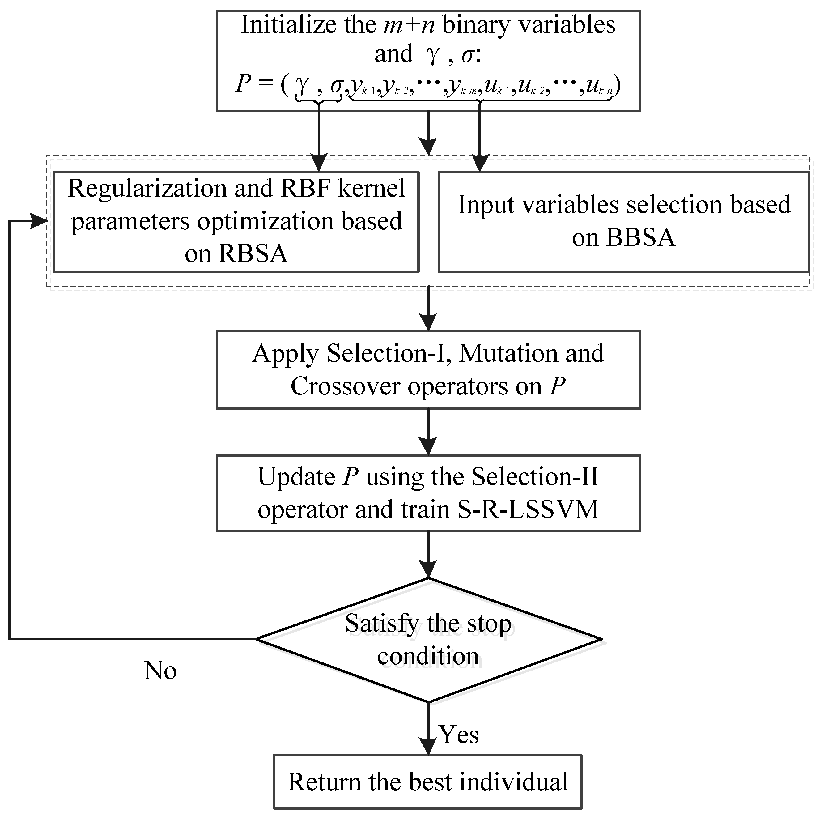
The steps of the HBSA-S-R-LSSVM identification model are as follows:

Step 1: Data preparation and initialization. Normalize the original data to [0, 1] and divide it into a training data set and a test data set. Determine the initial candidate input variables. Initialize the population size of the HBSA as N, the dimension of the individuals in the population as n + m + 2, and the maximum iteration number as G;

Step 2: Randomly generate the initial population. The i-th individual in the j-th iteration can be expressed as $L_i\left(j\right) ,i=1,2,\dots ,N,j=1,\mathrm{2...},G$, where the regularization parameter γ and radial basis function (RBF) kernel parameter σ are expressed in real numbers, and the candidate input variables are expressed in ‘0’ or ‘1’;

Step 3: Calculate the fitness value of the individuals according to Equation (23);

Step 4: Randomly generate the historical population OldP, update the historical population according to the selection-I operator, and obtain the initial experimental population T based on the mutation operator;

Step 5: Generate a search direction matrix map and obtain the final experimental population according to the crossover operator;

Step 6: Calculate the fitness value of the individuals in the current population and update the population according to the selection-II operator;

Step 7: If the number of iterations $j<G$, go to step 3; otherwise, go to the next step;

Step 8: Select the best individual $L_{best}$. The optimal input variables are selected from the predefined n + m candidate input variables, and the optimal parameters of the S-R-LSSVM model are optimized using the training data. The predicted value is obtained using the test data. The final output can be obtained after reversing the normalization.

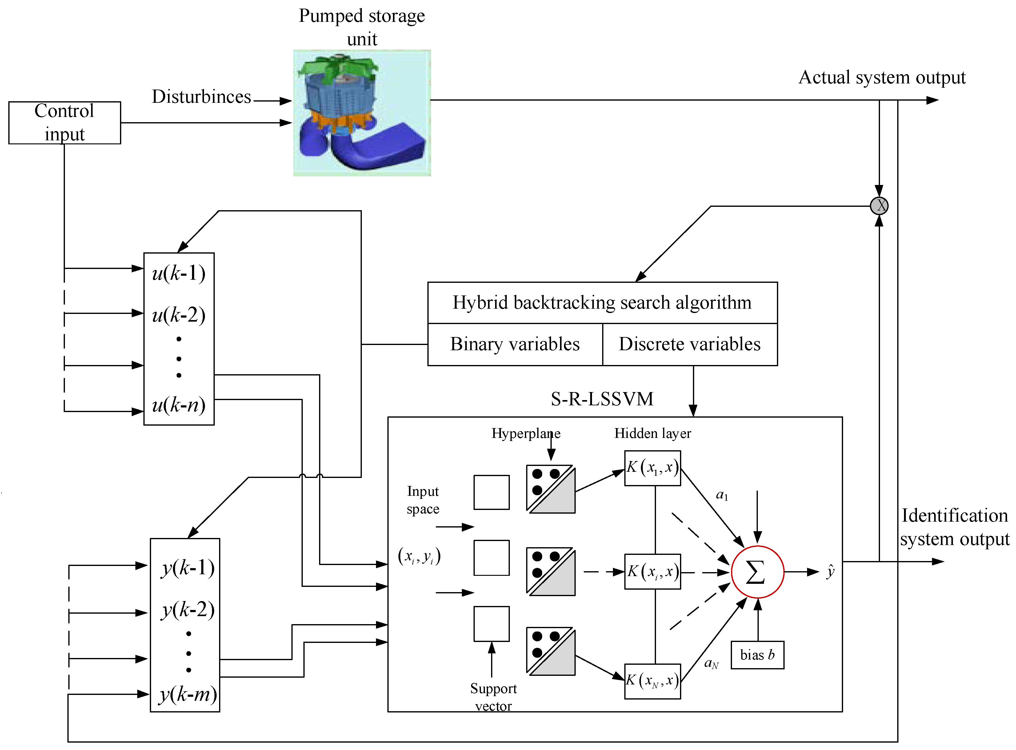
The optimization process of the HBSA to optimize the S-R-LSSVM model is shown in Figure 2. The structure of the S-R-LSSVM identification model optimized by the HBSA for the PTGS is shown in Figure 3.

4. Application to Benchmark Problems

Since the two nonlinear systems, including the SinC mathematical function and a nonlinear differential equation, contain a small number of candidate input variables, there is no need to use the synchronous optimization strategy. The S-R-LSSVM model is employed for the model identification of the two nonlinear systems. The identification result of the S-R-LSSVM model has been compared with those of the other existing models, including the extreme learning machine (ELM), LSSVM, and WLSSVM models. The RMSE, the mean absolute error (MAE), and the mean absolute percent error (MAPE) [21,33] are exploited as model performance evaluation indices to access the model identification accuracy.

4.1. SinC Mathematical Function

In this subsection, the Singer function SinC is taken as the first benchmark problem. The Singer function is the product of the sine function sinx and the monotonically decreasing function 1/x. The mathematical expression of the Singer function SinC is as follows:

$$\mathrm{SinC}\left(x\right)=\frac{\sin \left(x\right)}{x}$$

(24)

First, 200 points uniformly generated in [−10,10] are taken as the input variable x of the identification model. The corresponding output values are then calculated and taken as the output variable y. The 200 points $\left\{\left(x_i,y_i\right),i=1,2,\dots ,200\right\}$ construct the training samples for model identification. In order to verify the generalization capability of the S-R-LSSVM model, 240 points uniformly generated in [−12,12] are taken as the test data.

The Gauss white noise with 0 mean and 0.02 variance is added to the targeted output of the training data. Different proportions of training samples are randomly selected and converted to outliers by adding a certain proportion of disturbance to the original value. There are four schemes to add noise and outliers: Scheme A adds Gauss white noise to the expected output and selects 5% of the training samples to be converted to outliers; Scheme B adds Gauss white noise and selects 10% of the training samples; Scheme C adds Gauss white noise and selects 15% of the training samples; Scheme D adds Gauss white noise and selects 20% of the training samples to be converted to outliers.

After adding noise and outliers to the SinC function, the S-R-LSSVM, the ELM, the LSSVM, and the WLSSVM models are trained and tested. The parameters of the four different models are set as follows: the ELM model employed the Sigmoid function as a hidden activation function, and the number of hidden nodes is obtained through cycle verification; the RBF Gaussian function is employed as the kernel function in the models based on support vectors (LSSVM, WLSSVM, S-R-LSSVM), and the kernel parameter σ and regularization parameter γ are tuned through the grid search algorithm. 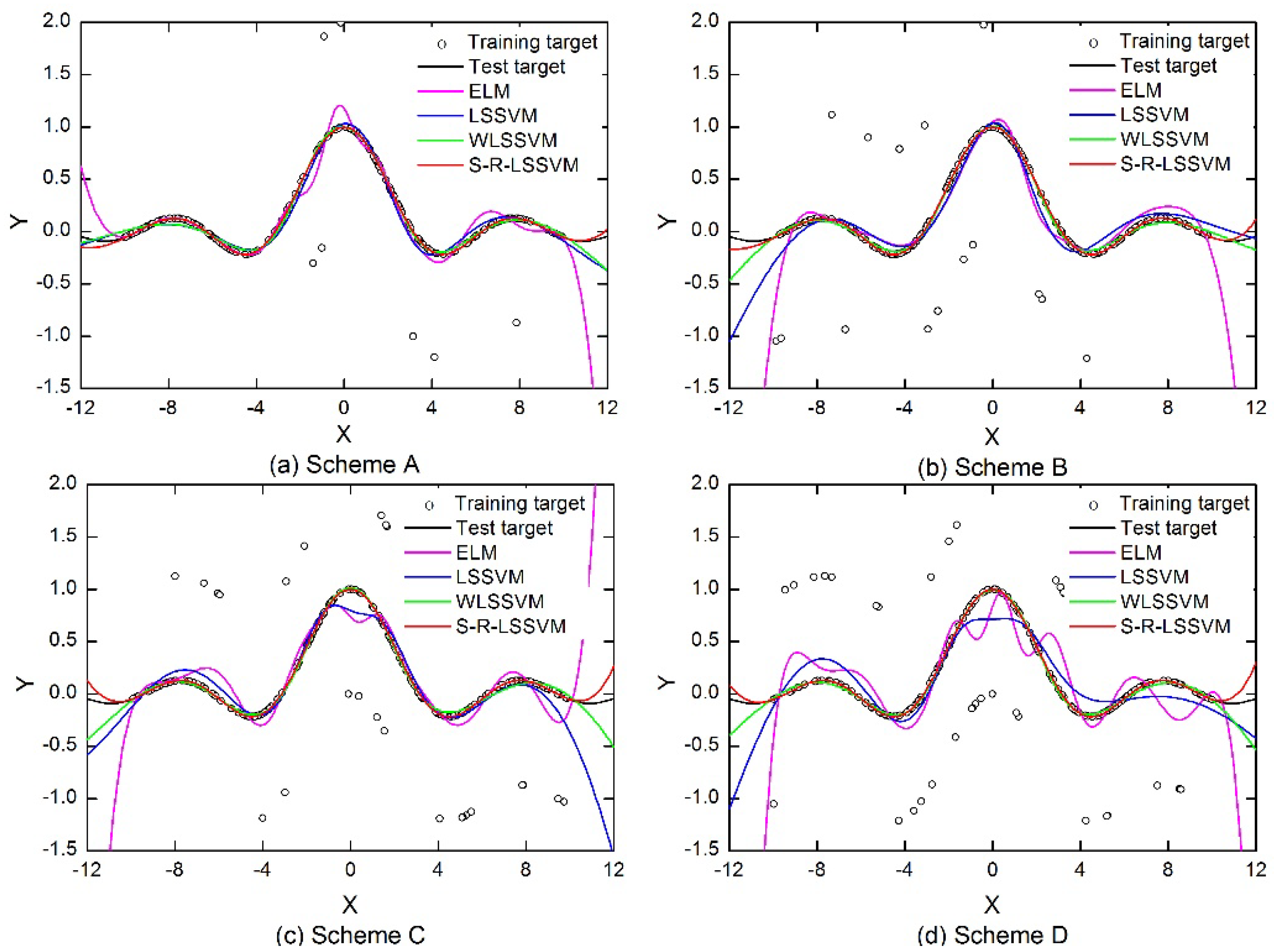The search range of γ is set as [2⁻⁸,2⁸], while the search range of σ is set as [2⁻⁶,2⁶]; the robust loss function recommended by Suykens [18] is employed in the WLSSVM; the weighting function based on improved normal distribution is employed in the S-R-LSSVM model. The ELM, LSSVM, WLSSVM, and S-R-LSSVM models are exploited to simulate the SinC function using data samples adding Gaussian white noises and outliers in four different schemes. A comparison between the predicted and actual values is shown in Figure 4, where the discrete points around the SinC function curve are outliers of the training sample set.

Table 1. Comparison of the test results for SinC function. ELM: extreme learning machine, LSSVM: least squares support vector machine, WLSSVM: weighted LSSVM, RMSE: root mean square error, MAE: mean absolute error, MAPE: mean absolute percent error.

Models	5%			10%			15%			20%
	RMSE	MAE	MAPE	RMSE	MAE	MAPE	RMSE	MAE	MAPE	RMSE	MAE	MAPE
ELM	0.462	0.160	2.53	1.123	0.433	7.48	1.268	0.497	7.80	2.141	0.728	12.20
LSSVM	0.071	0.052	0.91	0.206	0.122	2.48	0.225	0.161	2.68	0.296	0.152	2.70
WLSSVM	0.056	0.033	0.61	0.070	0.035	0.63	0.093	0.046	0.85	0.092	0.042	0.78
S-R-LSSVM	0.019	0.007	0.11	0.028	0.010	0.15	0.045	0.013	0.21	0.046	0.013	0.20

shows the performance evaluation indices of each model in the test stage.

It can be seen from Table 1 that the test results of the S-R-LSSVM model are better than those of the other models for all four schemes. The WLSSVM model performed the second best among all the models, and the ELM model performed the worst. As can be seen from Figure 4, the proposed S-R-LSSVM model can predict the SinC function and approximate the actual value with better accuracy for all four schemes. It can also be seen from Figure 4d that even if a large amount of noise and outliers are added, the S-R-LSSVM model can still obtain great identification accuracy and generalization ability.

A detailed analysis of Table 1 shows that the error of the ELM model is far greater than that of the other models when adding a different amount of noises and outliers, which indicates that the ELM model has the worst extrapolation ability. It can also be seen from Figure 4 that the performance of the ELM model at the two ends of [−12,12] interval is very poor, and the trend of the target curve cannot be accurately tracked using ELM, which indicates that the ELM model is very sensitive to training data containing outliers. Although the identification accuracy of the LSSVM model is slightly better than that of the ELM model, the improvement of the modeling accuracy is limited. The prediction results of the WLSSVM model are better than the ELM and LSSVM models, and can better approximate the actual values. This is because the sparsity and robustness of the WLSSVM model can be improved through the pruning method and the error weighting function. The S-R-LSSVM model can effectively weaken the influence of the outliers on modeling accuracy and improve the robustness of the model. The identification accuracy and the generalization ability of the S-R-LSSVM model in the test stage is the best, which demonstrates the excellent environmental adaptability of the S-R-LSSVM model.

4.2. A Nonlinear Differential Equation

To further compare the modeling and identification performance of each model, a nonlinear differential equation is taken as the second benchmark problem. The nonlinear differential equation has been widely used in system identification [34,35,36]. The mathematical expression of the nonlinear differential equation is given as follows:

$$y\left(k+1\right)=\frac{y\left(k\right)y\left(k-1\right)y\left(k-2\right)u\left(k-1\right)\left(y\left(k-2\right)-1\right)+u\left(k\right)}{1+y^2\left(k-2\right)+y^2\left(k-1\right)}$$

(25)

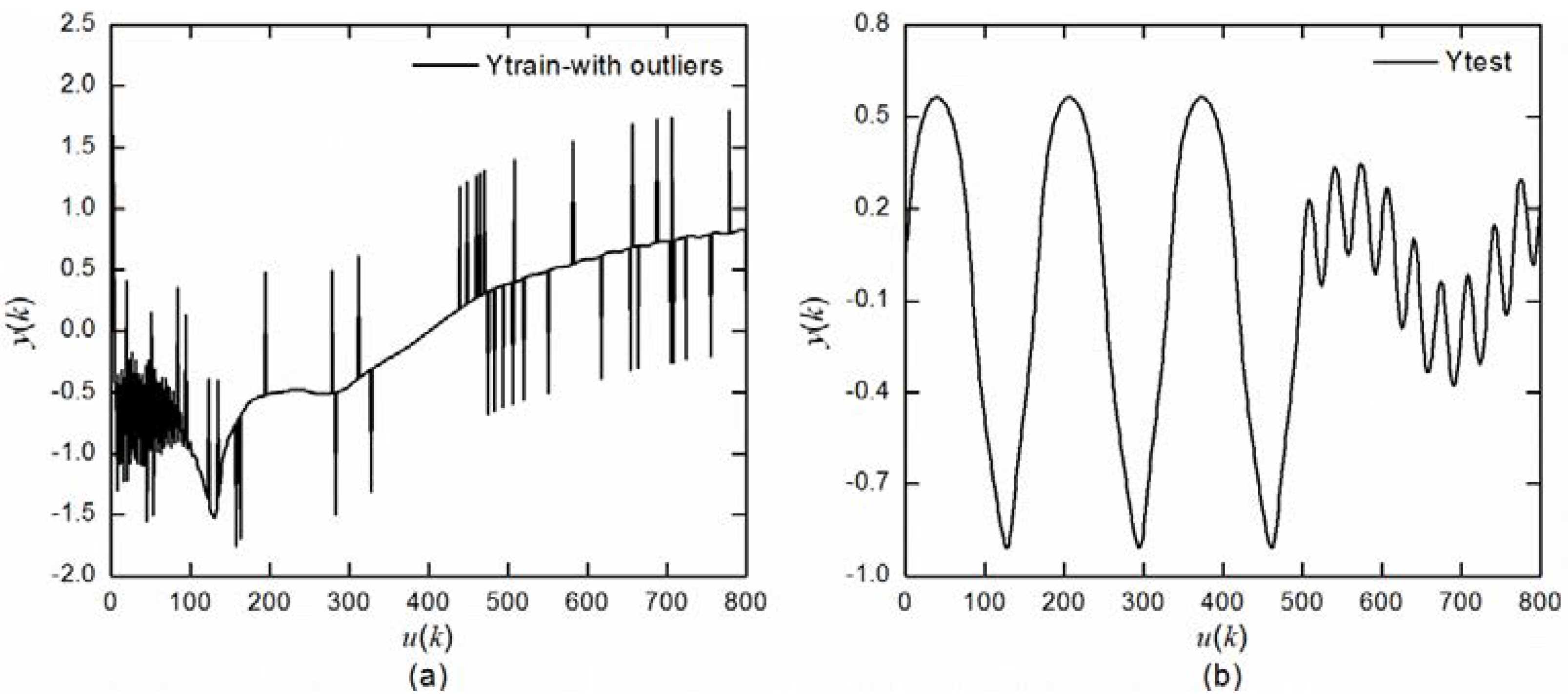
where $u\left(k\right)$ is the control input; and $y\left(k+1\right)$ is the output variable. First, 800 input-output data pairs randomly generated in [−2,2] according to Equation (25) are taken as the training samples. The function shown in Equation (26) is used to generate another 800 input–output data pairs as the test samples:

$$u\left(k\right)=\{\begin{array}{c}\sin \left(3\mathsf{\pi }k/250\right),k\le 500\\ 0.25\sin \left(2\mathsf{\pi }k/250\right)+0.2\sin \left(3\mathsf{\pi }k/50\right),k>500\end{array}$$

(26)

The input variables are adopted as $\left[y\left(k\right),y\left(k-1\right),y\left(k-2\right),u\left(k\right),u\left(k-1\right)\right]$, and the output variable is adopted as $y\left(k+1\right)$ for model identification. To verify the effectiveness of the S-R-LSSVM model, noise and outliers are added to the training samples according to the four schemes described in Section 4.1. The identification result of the S-R-LSSVM model is compared with those of the ELM, LSSVM, and WLSSVM models. 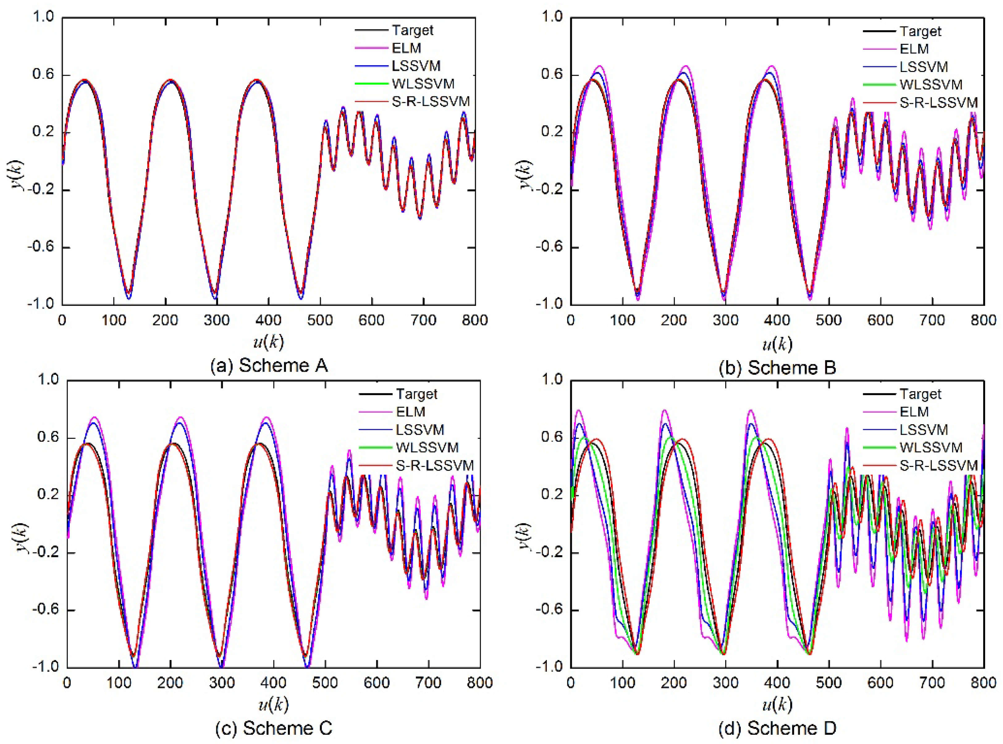The target output with noise and outliers in the training stage and the target output in the test stage are shown in Figure 5a,b, respectively. The forecasting results of the four different models in four different schemes are shown in Figure 6. The performance evaluation indices of each model are shown in

Table 2. Comparison of the test results for the nonlinear differential equation.

Models	5%			10%			15%			20%
	RMSE	MAE	MAPE	RMSE	MAE	MAPE	RMSE	MAE	MAPE	RMSE	MAE	MAPE
ELM	0.059	0.051	52.33	0.142	0.128	94.38	0.184	0.164	133.08	0.355	0.311	293.86
LSSVM	0.053	0.046	47.16	0.077	0.069	46.62	0.130	0.116	94.10	0.272	0.237	230.37
WLSSVM	0.023	0.021	17.19	0.022	0.019	17.99	0.033	0.030	20.54	0.133	0.118	93.27
S-R-LSSVM	0.019	0.017	13.86	0.017	0.015	13.33	0.038	0.034	23.33	0.079	0.070	58.38

.

Similar conclusions can be obtained as the SinC mathematical function. In all four schemes to add noises and outliers, the S-R-LSSVM model achieved greater modeling accuracy and generalization ability compared with the other three models. The predicted outputs of the ELM and LSSVM models deviated from the target values because they are sensitive to noises and outliers. The WLSSVM model can reduce the influence of noises and outliers to some extent through the error weighting function. Taking Scheme A, of which the proportion of outliers is 5% as an example, the RMSE of the S-R-LSSVM is as low as 0.019, which is a little higher than the 0.023 value of WLSSVM and much higher than the 0.053 value of LSSVM and 0.059 value of ELM. As can be seen from Figure 6, the S-R-LSSVM model has better anti-interference ability and can model the nonlinear dynamic system effectively under four different schemes to add noises and outliers. In particular, it is known from Figure 6d that the model still has great identification accuracy and generalization ability when a large amount of noise and outliers are added.

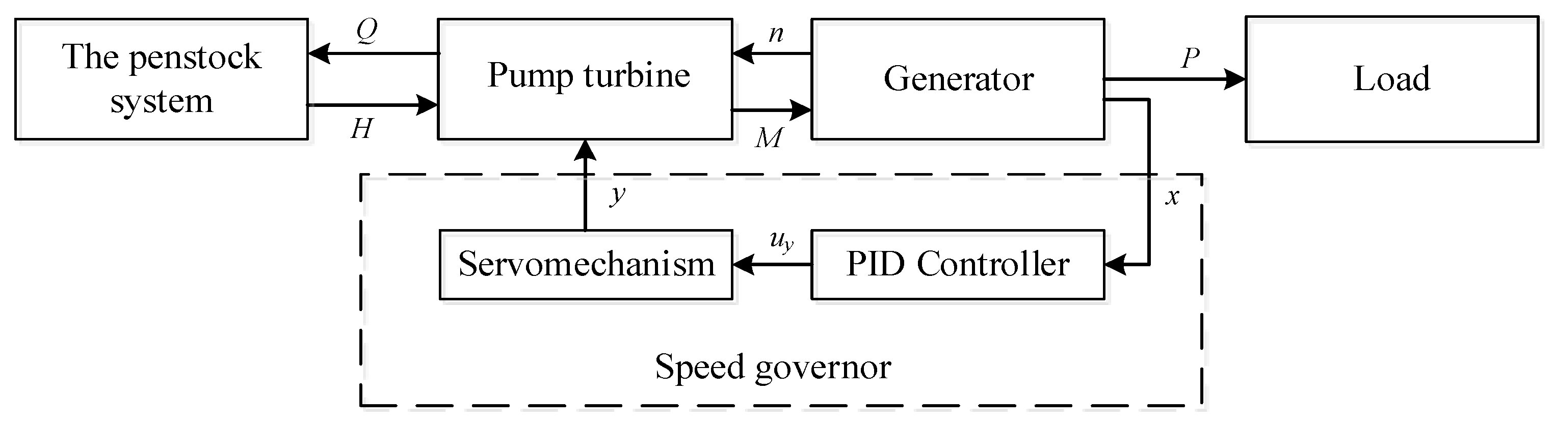
5. Application to Pump Turbine Governing System

The third nonlinear system is an application to the PTGS. The PTGS is a complicated closed-control system of the PSU that contains four parts: a speed governor, a penstock system, a pump turbine, and a generator with a load. The speed governor contains a servomechanism and a PID controller to control the guide vane opening. For more details about the four different parts of the PTGS, please refer to Li et al. [11] and Zhou et al. [37]. The schematic of PTGS is shown in Figure 7 [37].

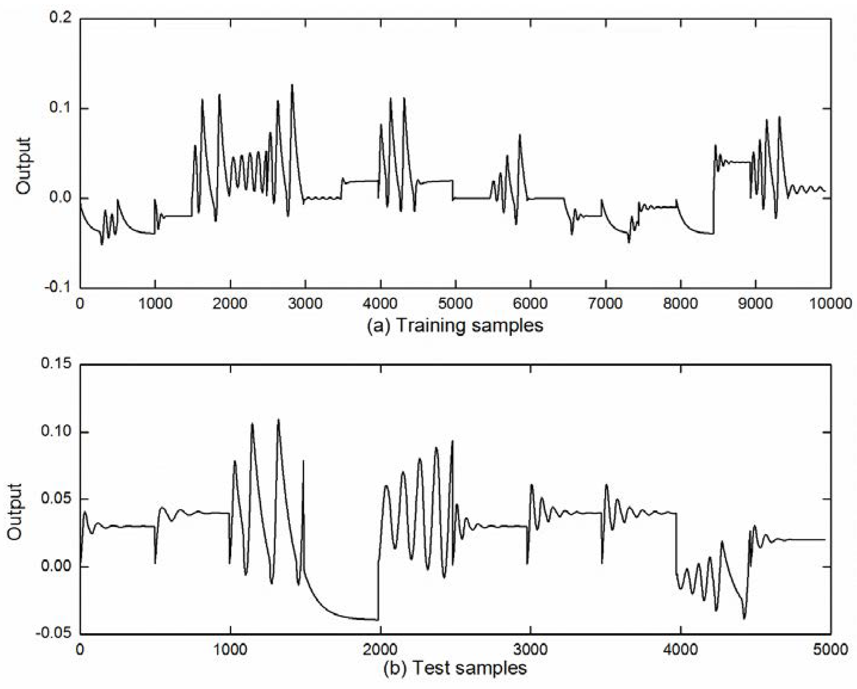
In this study, the S-R-LSSVM identification model is built to capture the nonlinear dynamic characteristic of the PTGS in a pumped storage power station in China. In the model identification process of the PTGS using the S-R-LSSVM model, the number of the candidate input variables is much larger. The synchronous optimization strategy based on the HBSA is then employed to optimize the number of input variables and the parameters of the S-R-LSSVM model (recorded as HBSA-S-R-LSSVM) at the same time. The identification result of the proposed HBSA-S-R-LSSVM model has been compared with those of the other existing models, including ELM, LSSVM, WLSSVM, S-R-LSSVM, and HBSA-LSSVM to demonstrate the effectiveness of the HBSA-S-R-LSSVM identification model. Considering the frequency disturbance of the PTGS is a common working condition in the actual operation of the PSU, and is also an experimental project that must be carried out after the completion of unit maintenance; the PTGS nonlinear dynamic model is excited using the frequency disturbance. The actual input–output data pairs of the PTGS are collected as modeling sample data for constructing the HBSA-S-R-LSSVM identification model.

The frequency disturbance signals of the PTGS are randomly generated, and the parameters of the PID controller are randomly set to fully describe the nonlinearity of PTGS and improve the diversity of training samples [10]. The simulation time is set as 50 s, and the sampling period is set as 0.1 s. The controller output and unit frequency output data of the PTGS are preserved at the end of each experiment. A total number of 30 independent experiments under frequency disturbance are performed, of which 20 of the dynamic processes of the experiments are taken as training samples, and the remaining 10 experiments are taken as test samples. Illustrations of the training samples and the test samples are shown in Figure 8.

In order to verify the effectiveness of the S-R-LSSVM model and the synchronous optimization strategy based on the HBSA, model identification experiments of the PTGS with Gaussian white noise and 5% outliers (Scheme A), as well as Gaussian white noise and 10% outliers (Scheme B), were constructed. A total number of six models were constructed for PTGS model identification. The six models can be grouped into three categories as follows:

(1) Identification models in which the model structure and parameters are optimized separately. These models include the ELM, LSSVM, WLSSVM, and S-R-LSSVM models. The input variables are adopted as $\left\{u\left(t-1\right),u\left(t-2\right),u\left(t-3\right),y\left(t-1\right),y\left(t-2\right),y\left(t-3\right)\right\}$ according to Li et al. [10,11]. The model parameters are optimized in the same way as the two nonlinear benchmark problems;

(2) The LSSVM identification model in which the model structure and parameters are optimized synchronously using the HBSA (recorded as HBSA-LSSVM). The candidate input variables to be optimized are $\left\{u\left(t-1\right),\dots ,u\left(t-6\right),y\left(t-1\right),\dots ,y\left(t-6\right)\right\}$. The population size of the HBSA is 40, and the number of iterations is 200;

(3) The S-R-LSSVM identification model in which the model structure and parameters are optimized synchronously using the HBSA (HBSA-S-R-LSSVM). The parameters of the HBSA are set as the same as the HBSA-LSSVM.

Experiments of the above six identification models under different proportions of noises and outliers are carried out. The identification results of different models for PTGS in the test stage are given in

Table 3. Comparison of the test results for PTGS model identification.

Models	5%			10%
	RMSE	MAE	MAPE	RMSE	MAE	MAPE
ELM	6.64 × 10−3	3.43 × 10−3	4.47 × 10−1	1.10 × 10−2	7.07 × 10−3	9.49 × 10−1
LSSVM	3.73 × 10−3	2.96 × 10−3	3.84 × 10−1	7.12 × 10−3	5.61 × 10−3	7.59 × 10−1
WLSSVM	1.72 × 10−4	8.36 × 10−5	1.14 × 10−2	1.93 × 10−4	8.44 × 10−5	1.32 × 10−2
S-R-LSSVM	8.21 × 10−5	2.60 × 10−5	5.30 × 10−3	8.24 × 10−5	2.66 × 10−5	5.52 × 10−3
HBSA-LSSVM	3.57 × 10−3	2.30 × 10−3	1.40 × 10−1	6.34 × 10−3	5.48 × 10−3	5.12 × 10−1
HBSA-S-R-LSSVM	5.99 × 10−5	1.93 × 10−5	3.89 × 10−3	5.97 × 10−5	2.18 × 10−5	3.90 × 10−3

.

From the results of Table 3, it can be seen that for the four identification models in which the model structure and parameters are optimized separately, the performance of the ELM model based on empirical risk minimization is the worst, for it is very sensitive to noises and outliers. The LSSVM model based on structural risk minimization can improve the model identification accuracy to a certain extent, but the perdition accuracy and generalization ability are still insufficient. It can be seen from the comparison of the LSSVM and WLSSVM models that the identification result of the WLSSVM is significantly better than that of the LSSVM, which indicates that the WLSSVM has strong anti-jamming ability and can effectively reduce the prediction error. The results of the S-R-LSSVM identification model are relatively stable under both schemes to add noises and outliers. The prediction accuracy and robustness are superior to the other models, which indicates that the sparseness and robustness strategies of the identification model can reduce the influences of noise and outliers on modeling accuracy and stability. For identification models using the synchronous optimization strategy based on the HBSA, the input variables are selected as $\left\{u\left(t-1\right),u\left(t-2\right),u\left(t-4\right),y\left(t-1\right),y\left(t-2\right),y\left(t-3\right),y\left(t-6\right)\right\}$ using the HBSA. The performance of the models with a synchronous optimization strategy have been improved compared with those without a synchronous optimization strategy. Taking the S-R-LSSVM and HBSA-S-R-LSSVM models under Scheme A as an example, the RMSE is reduced from 8.21 × 10⁻⁵ to 5.99 × 10⁻⁵, the MAE is reduced from 2.60 × 10⁻⁵ to 1.93 × 10⁻⁵ and the MAPE is reduced from 5.30 × 10⁻³ to 3.89 × 10⁻³ using the HBSA. The performance evaluation indices of the HBSA-S-R-LSSVM model are smaller than all of the other models under the two schemes to add noises and outliers, which indicate that the HBSA-S-R-LSSVM can effectively improve the accuracy of PTGS model identification. 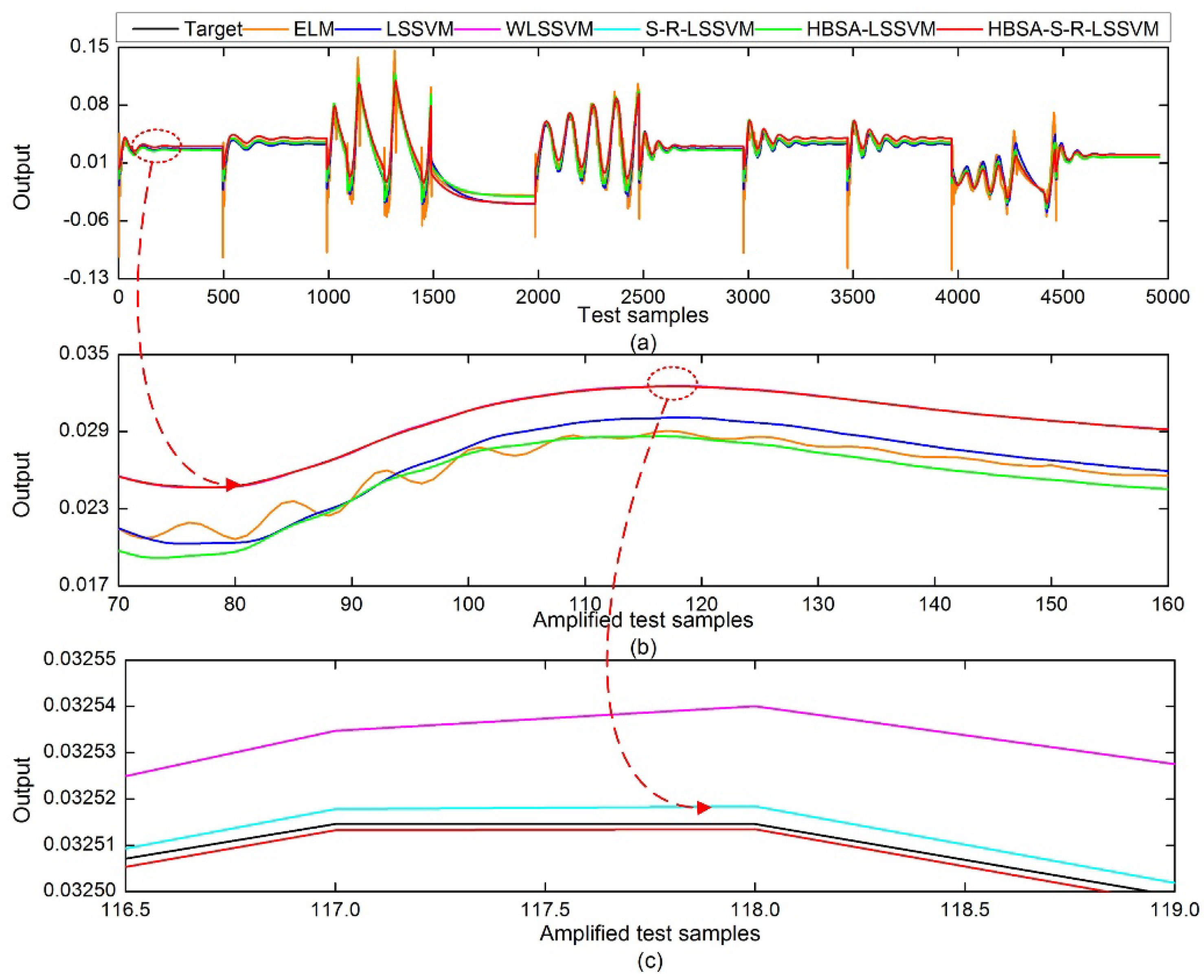Figure 9 and Figure 10 compare the predicted output of each identification model with the targeted output under Scheme A and Scheme B, respectively. 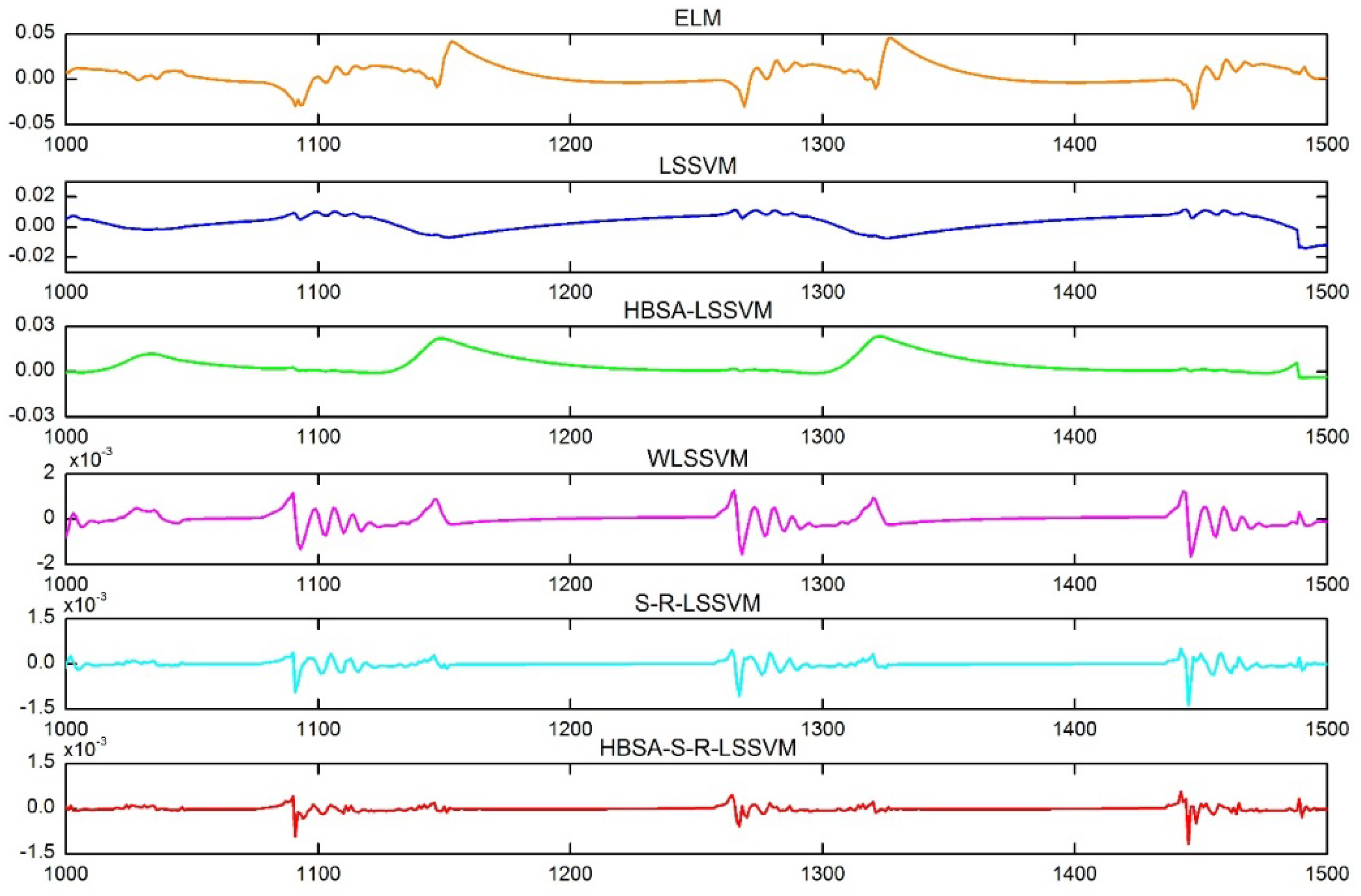Figure 11 shows the predicted residuals for each identification model under Scheme A.

It can be seen in Figure 8, Figure 9 and Figure 10 that the performances of the ELM and LSSVM models are severely affected by noise and outliers. The WLSSVM, S-R-LSSVM, and HBSA-S-R-LSSVM models with anti-jamming ability can better track the actual changes of the targeted output. Compared with identification models without a synchronous optimization strategy, the predicted outputs of the models based on the HBSA are more consistent with the targeted output, and the predicted residual is smaller. The identification accuracy of the proposed HBSA-S-R-LSSVM model is the highest, which demonstrates that the proposed model can well track the changes in unit frequency and capture the nonlinear dynamic characteristics of the system.

6. Conclusions

This study proposes an HBSA-S-R-LSSVM model for the model identification of the PTGS. The sparsity of the support vectors of the LSSVM model is realized using the maximum linearly independent set, while the robustness of the model is enhanced using the robust weighting function based on improved normal distribution function. The experimental results of a SinC mathematical function and the nonlinear differential equation show that the S-R-LSSVM identification model can enhance the robustness of the LSSVM model to noise and outliers. Considering that the model structure determination and the model parameters optimization can interact with each other, a binary-real coded HBSA algorithm is proposed to synchronously optimize the model input variables, the kernel parameters, and the regularization parameters. The identification results of a real-world application of the PTGS in a pumped storage power station in China show that the proposed HBSA-S-R-LSSVM model can ensure the model accuracy while enhancing the model robustness and generalization performance simultaneously.

Abbreviation

PSU	pumped storage unit
PTGS	pump turbine governing system
T-S	Takagi-Sugen
CAR	controlled auto-regressive
HTGS	hydraulic turbine governing system
NNARX	neural networks nonlinear autoregressive network with exogenous signal
MAPE	mean absolute percent error
MAE	mean absolute error
LSSVM	least squares support vector machine
S-R-LSSVM	sparse robust LSSVM
WLSSVM	weighted LSSVM
ELM	extreme learning machine
HBSA	hybrid backtracking search algorithm
ANFIS	adaptive network-based fuzzy inference system
RMSE	root mean square error