Parametric Studies for Combined Convective and Conductive Heat Transfer for YASA Axial Flux Permanent Magnet Synchronous Machines

Abstract

In this paper, the effect of some geometrical parameters on the steady state average temperature of the stator core, the winding and the permanent magnets of the yokeless and segmented armature (YASA) axial flux permanent magnet synchronous machine (AFPMSM) is studied. The geometrical parameters selected for the study are the air gap length, the inward heat extraction fin thickness and the permanent magnet thickness. These parametric studies make it possible to obtain a better trade-off between power density and efficiency. These investigations are very helpful in correlating the values of the geometrical parameters to some specific desired performance criteria like not going below some desired minimum efficiency, limiting the temperature of specific part to some maximum value for maximization of lifetime and also determination of the allowed speed range to limit the temperatures lower than the critical values. This is important specifically for the synchronous machines due to the fact that the speed value affects both the losses and the heat transfer convection coefficients. The air gap length has a direct effect on the overall machine losses and the air gap convection coefficient and hence on the temperature of the machine. As the fins are between the stator windings, a thicker fin reduces the space for copper windings and hence increases the losses, but at the same time improves heat evacuation. In addition, the effect on the temperature is studied of the speed variation, which influences both the losses and the convection coefficients of the machine. Every study is made based on coupled electromagnetic and thermal models. The results are obtained from analytical electromagnetic and thermal models verified by finite element simulations and validated experimentally on a 4 kW yokeless and segmented armature axial flux machine.

1. Introduction

Many types of axial flux permanent magnet synchronous machines exist. These types differ in the number of stators and rotors and the location of them in the machine. Some of these types are axial flux internal rotor (AFIR), toroidally wound internal stator (TORUS), axial flux internal stator (AFIS) and yokeless and segmented armature (YASA) [1]. The absence of the stator yoke in the YASA type makes it more efficient. The complete design and optimization of the YASA machine needs accurate electromagnetic, thermal and mechanical models for the machine. The electromagnetic models are mainly providing the magnetic field distribution in the machine parts. Based on the calculated magnetic field distribution, many important quantities can be calculated. The developed torque, the cogging torque, the induced voltage, the permanent magnets losses and the core losses are some of these quantities [2]. Two main methods for the electromagnetic modeling exist: the finite element method (FEM) and the analytical method. The 3D FEM modeling method is the most accurate and the most time-consuming one [3,4,5]. Another quasi-3D FEM method is used in which the machine is divided into slices in the radial direction, the flux density distribution is calculated for every slice and then summation is done to obtain the total flux. This method provides a good compromise between the accuracy and the solution time [2,6]. The magnetic equivalent circuit (MEC), the analytical solutions of Maxwell’s equations and the combination of them are the analytical electromagnetic modeling methods [7,8,9].

For thermal modeling, the FEM and the lumped parameter thermal network method (LPTN) represent the numerical and the analytical thermal modeling methods. Refs. [10,11,12,13] are some of the papers presenting the FEM thermal modeling technique for the YASA machine while [14,15,16] studied the LPTN modeling method. The LPTN method has the advantage of being fast enough while, on the other hand, the FEM method provides a more detailed temperature distribution in every part. In this paper, the effect of the air gap length, the speed, the heat extraction fins thickness and the permanent magnet (PM) thickness on the machine losses and the temperature is studied. The coupling between the electromagnetic model and the thermal model is necessary for the studies in this paper for two reasons. The first one is the dependence of the machine losses on the values of the studied parameters and the second one is the temperature dependent material properties [17].

2. YASA Electromagnetic Models

The electromagnetic model must be able to accurately compute several loss terms as a function of the studied parameters: winding loss, the iron loss, and the loss in the permanent magnets. These losses are the sources of the thermal model in Section 3.

The analytical electromagnetic model (EM) adopted for parametric studies in this paper is the quasi-3D modeling technique combined with the magnetic equivalent circuit [2].

The core losses are calculated using the method of loss separation (1) [18]:

$$\begin{array}{c}{P}_{loss}=(P_{hys}+P_{classic}+P_{excess})\rho ,\hfill \\ P_{hys}=K_1{B_p}^{k_2}f,\hfill \\ P_{class}\left(t\right)=K_3{\left(\frac{dB}{dt}\right)}^2,\hfill \\ P_{excess}\left(t\right)=K_4(\sqrt{1+k_5\left|\frac{dB}{dt}\right|}-1)\frac{dB}{dt},\hfill \end{array}$$

(1)

where $P_{loss}$ is the power loss W/m${}^3$, $P_{hys}$ is the hysteresis losses, $P_{classic}$ is the classic loss, $P_{excess}$ is the excess loss, $\rho$ is the mass density, ($K_1$–$K_5$) are material dependent constants, and f is the frequency $B_p$ is the peak flux density.

For the PM losses, the method developed in [6] is adopted here.

The dependency of the core and PM losses on the frequency is clear. Remaining is the dependency of the winding losses on the frequency which comes from the skin and proximity effects. The AC resistance $R_{AC}$ can be calculated from (2) [19]:

$$\begin{array}{c}{t}_d=\frac{1}{\sqrt{\pi f{\mu }_o\sigma }},\hfill \\ K_r=\frac{d_c}{t_d},\hfill \\ G_b=K_r\frac{sinh2K_r+sin2K_r}{cosh2K_r-cos2K_r},\hfill \\ G_{br}=2K_r\frac{sinh{K}_r-sin{K}_r}{cosh{K}_r+cos{K}_r},\hfill \\ K_{in}=G_b+\frac{m^2-1}{3G_{br}},\hfill \\ R_{AC}=K_{in}\times R_{DC},\hfill \end{array}$$

(2)

where f is the frequency in Hz, $\sigma$ is the conductor conductivity in S/m, $t_d$ is the skin depth in meters, $d_c$ is the conductor diameter, m is the number of conductors along the axial length of the slot, $K_r$ is the ratio between the actual conductor diameter and the effective conductor diameter seen by the AC current flowing, $K_{in}$ is the ration between the AC and the DC resistances of the same conductor at certain frequency and $R_{DC}$ is the conductor resistance seen by a zero frequency current.

3. YASA Thermal Models

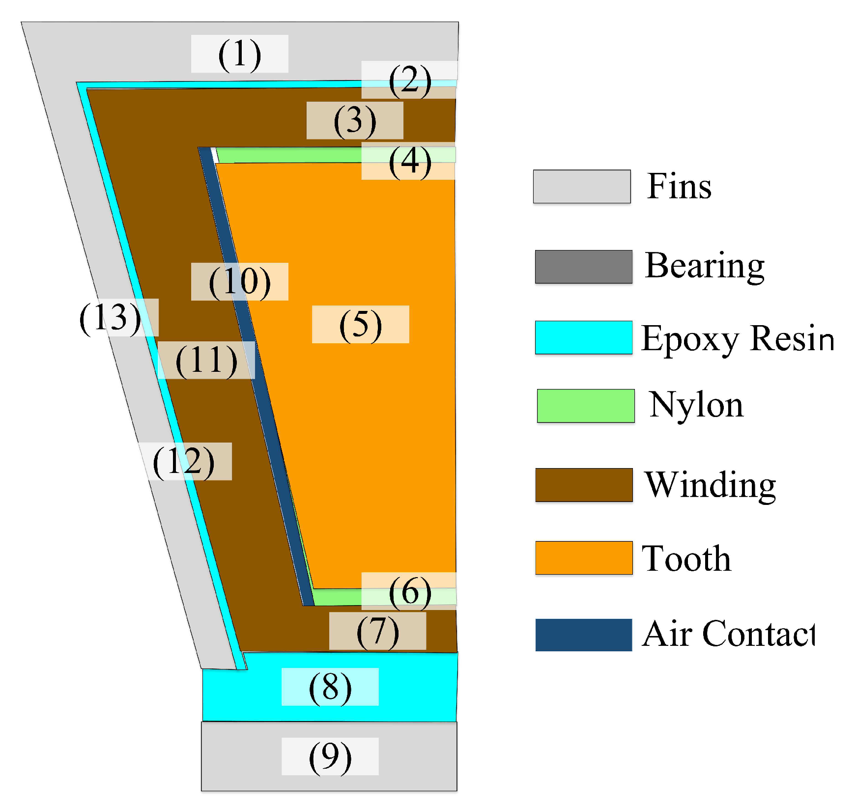
In this section, the analytical thermal model adopted for the coupling studies in this paper is discussed along with the FEM thermal model used to verify the results of the coupled models based studies in the next sections.

3.1. YASA LPTN

The lumped parameter thermal network (LPTN) is a network of thermal resistors, capacitors and heat sources. The solution of the network gives the average temperature of each element represented by a node in this network. The values of these resistors and capacitors are driven from the material properties and geometry of the machine under study. The geometry of the YASA machine under study is shown in Figure 1, while the material properties are given in

Table 1. Material properties.

Material	K (W/mK)	${\mathit{C}}_{\mathit{p}}$ (J/kgK)	$\mathit{\rho }$ (kg/m${}^3$)
copper	385	392	8890
aluminum	167	896	2712
epoxy	0.4	600	1540
nylon	0.25	1600	1140
Nd-Fe-B	9	500	7500

.

The details of the LPTN model developed by the authors and adopted for the study in this paper can be found in [16]. In this model, the rotor and the stator are represented by two different networks coupled by the analytical convection heat transfer coefficients in [20,21]. The analytical equations for the convection coefficients calculation take the form (3).

$$\begin{array}{c}G=\frac{2g}{D},\\ Re=\frac{\Omega D^2}{4\nu },\\ {\alpha }_m=\alpha \times \frac{N_m}{360},\\ L=\frac{t}{R}\\ \overline{N{u}_{h_i}}=Y_{h_i}(G,Re,{\alpha }_m,L),\\ \overline{h_i}=\frac{\overline{N{u}_i}k}{l_i},\end{array}$$

(3)

where g is the air gap length in m, D is the rotor disk diameter in m, $\Omega$ is the rotational speed in rad/s, $\nu$ is the kinematic viscosity of the air, $\alpha$ is the magnet angle, t is the magnet thickness, R is the rotor radius, $\overline{h_i}$ is the convection coefficient of the surface i, K is the air thermal conductivity and $l_i$ is the characteristic length of the air.

It is important to notice from equation (3) that the convection coefficients depend on the air gap length, rotational speed and the magnets’ geometrical parameters. This means that the change of these parameters, besides affecting the machine losses, also affects the convection coefficients. This makes the study of the variation of these parameters on the machine temperature very interesting and useful in the selection of these parameters.

The LPTN for the stator and the rotor is shown in Figure 2 and Figure 3, respectively.

The $T_{ref}$ indicated in the LPTN represents the temperature of a nearby volume of air close to the convected surface [20,21]. The value of this temperature depends on the average temperature of the stator $T_s$ and the rotor $T_r$ and also on the same parameters as the convection coefficients (4):

$$\begin{array}{c}{a}_{hi}=F_{hi}(G,Re,{\alpha }_m,L),\hfill \\ b_{hi}=G_{hi}(G,Re,{\alpha }_m,L),\hfill \\ {\overline{T}}_{{ref}_i}=a_i{T}_r+b_i{T}_s+(1-(a_i+b_i))T_a,\hfill \end{array}$$

(4)

where $T_a$ is the ambient temperature.

It is important to mention here that, due to symmetry and thermal periodicity, only one-quarter of one of the stator teeth is modeled and only one rotor PM. The LPTNs of the stator and the rotor are then solved to get the temperature of the machine.

3.2. 3D Thermal FEM Model

A 3D FEM model is developed to verify the results of the coupled electromagnetic-thermal analytical models based studies in the next sections. The modeled quarter tooth and rotor segment are shown in Figure 4a,b, respectively.

The boundary conditions used in the simulation are thermal insulation for parts parallel to the cutting plane and convective heat transfer for convected surfaces. The power losses of the different machine parts are assumed to be equally distributed on the volume.

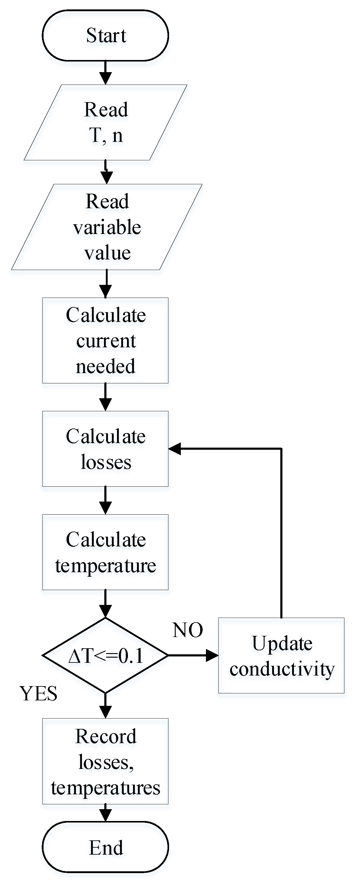
4. Coupled EM-Thermal Study

Both the electromagnetic and the thermal models are needed in this study to compute the losses from the electromagnetic models and the temperatures from the thermal model resulting from variation of the studied parameters. These models are coupled by the dependence of the winding resistivity on the temperature. The winding resistivity change is handled by solving the coupled models iteratively until stabilization of the temperature as in the flow chart in Figure 5.

5. The Parametric Studies

In this section, the resultant power losses, efficiency and the average steady state temperature variation of the winding, the core and the PMs with the air gap length, the speed, the inward heat extraction fins thickness and the PM thickness are studied. These studies are done on a 4 kW, 2500 rpm YASA machine with the geometrical parameters in

Table 2. YASA geometrical parameters.

Parameter	Value	Unit
number of poles	16	-
teeth number	15	-
outer diameter housing	195	mm
outer diameter active	148	mm
PM thickness	4	mm
rotor outer radius	74	mm
slot width	11	mm

.

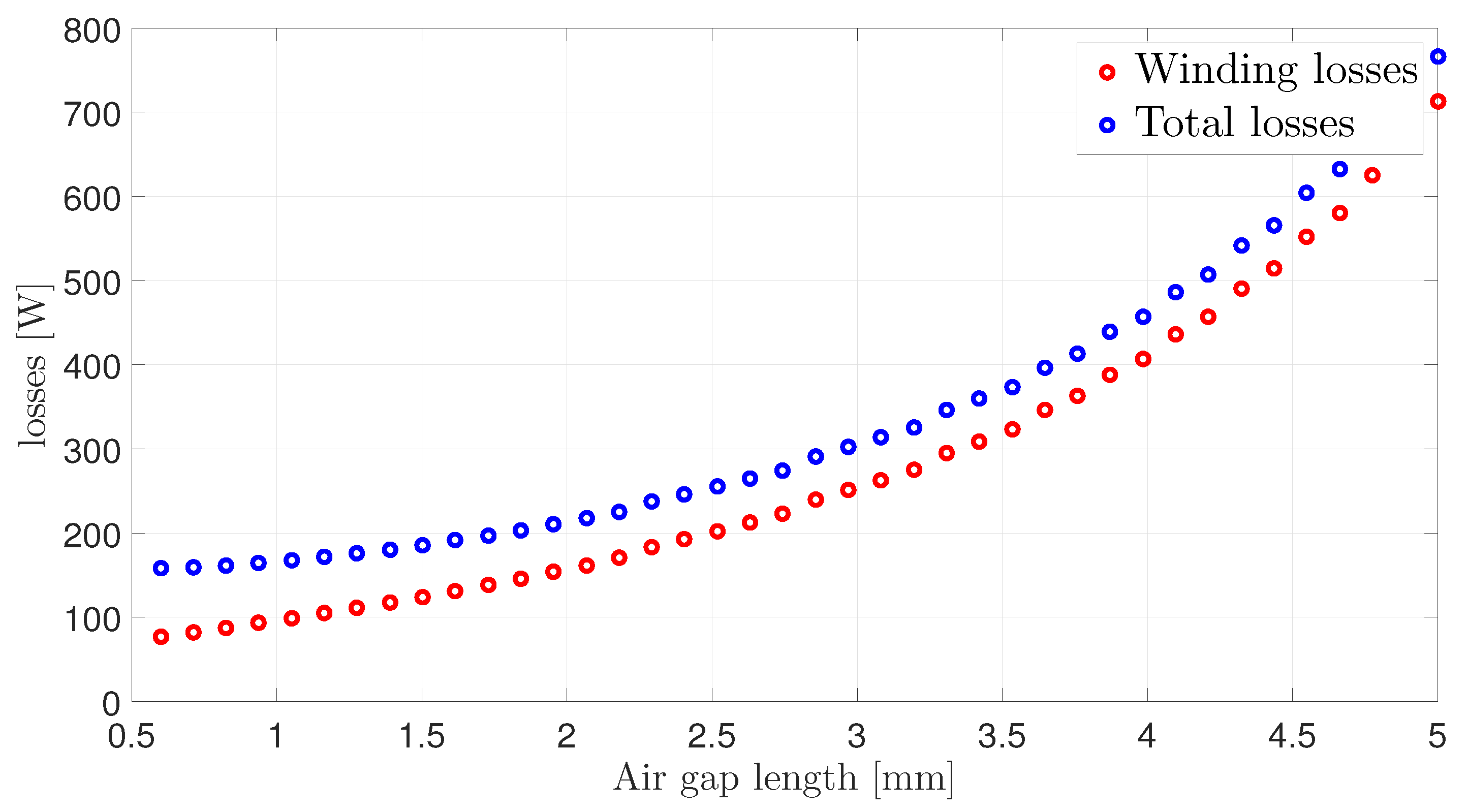
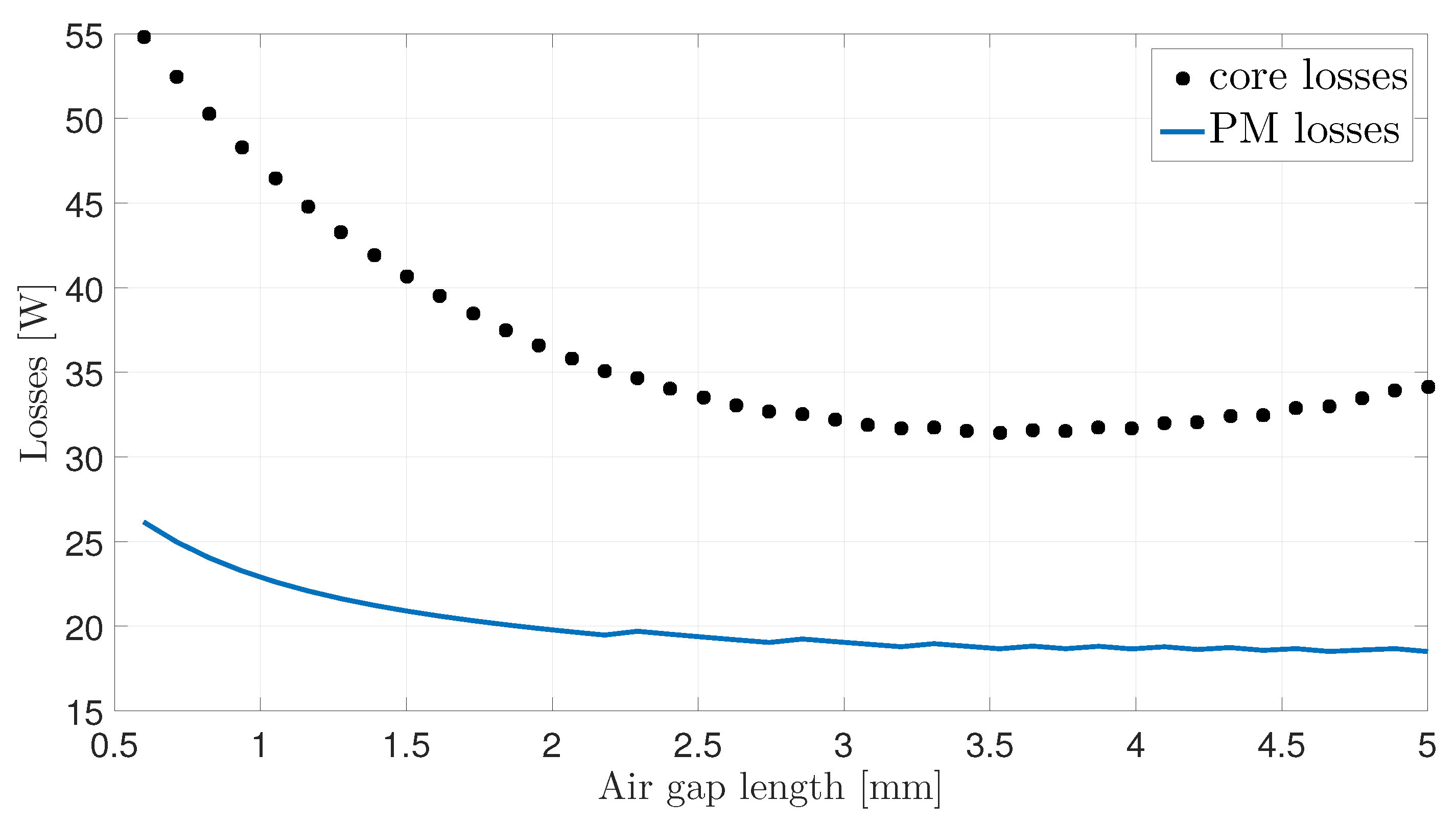
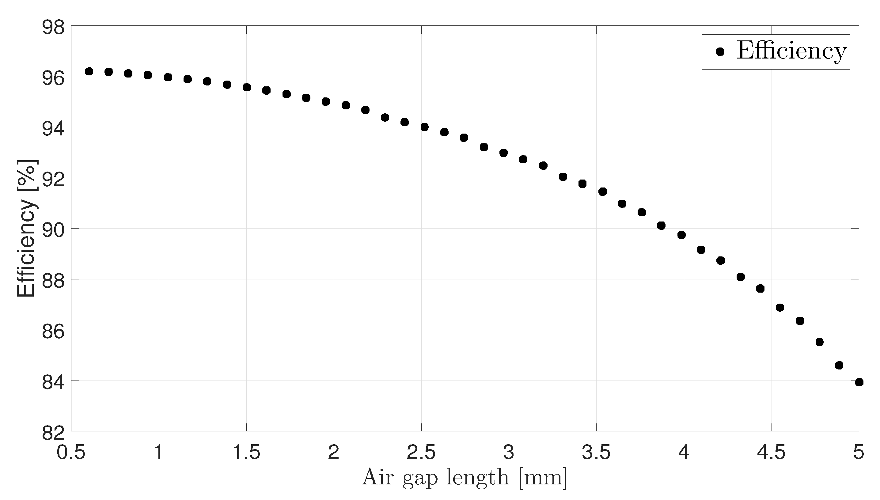
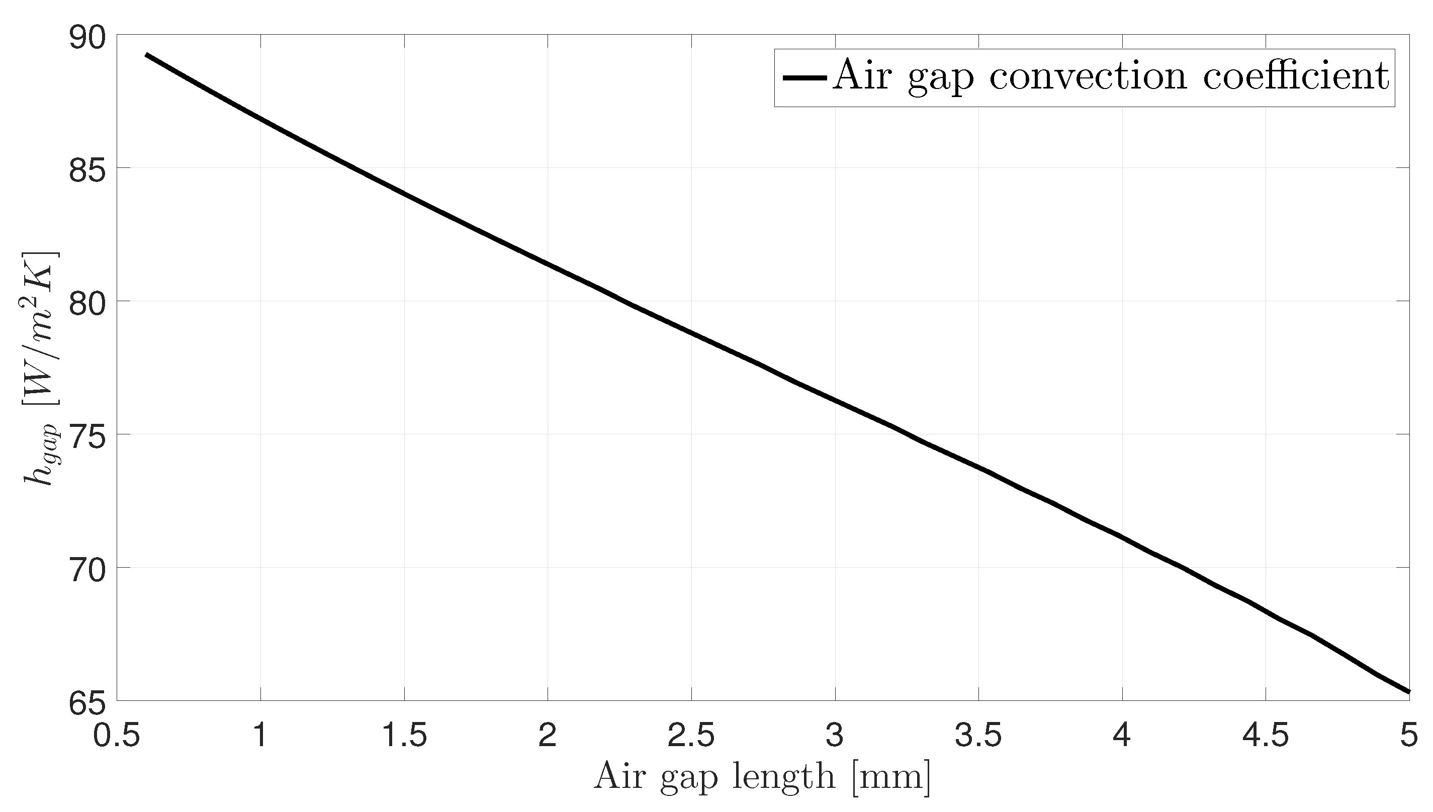
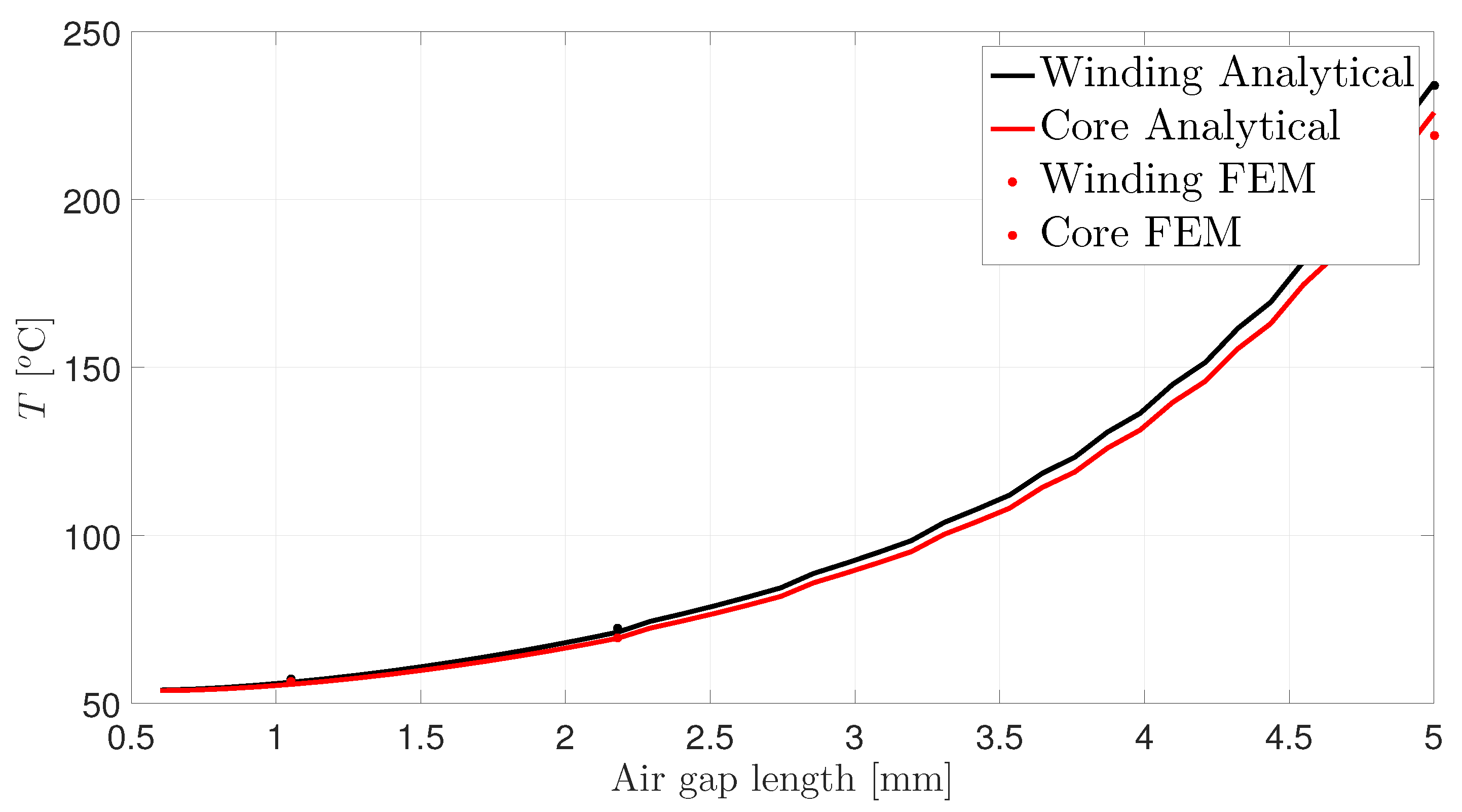
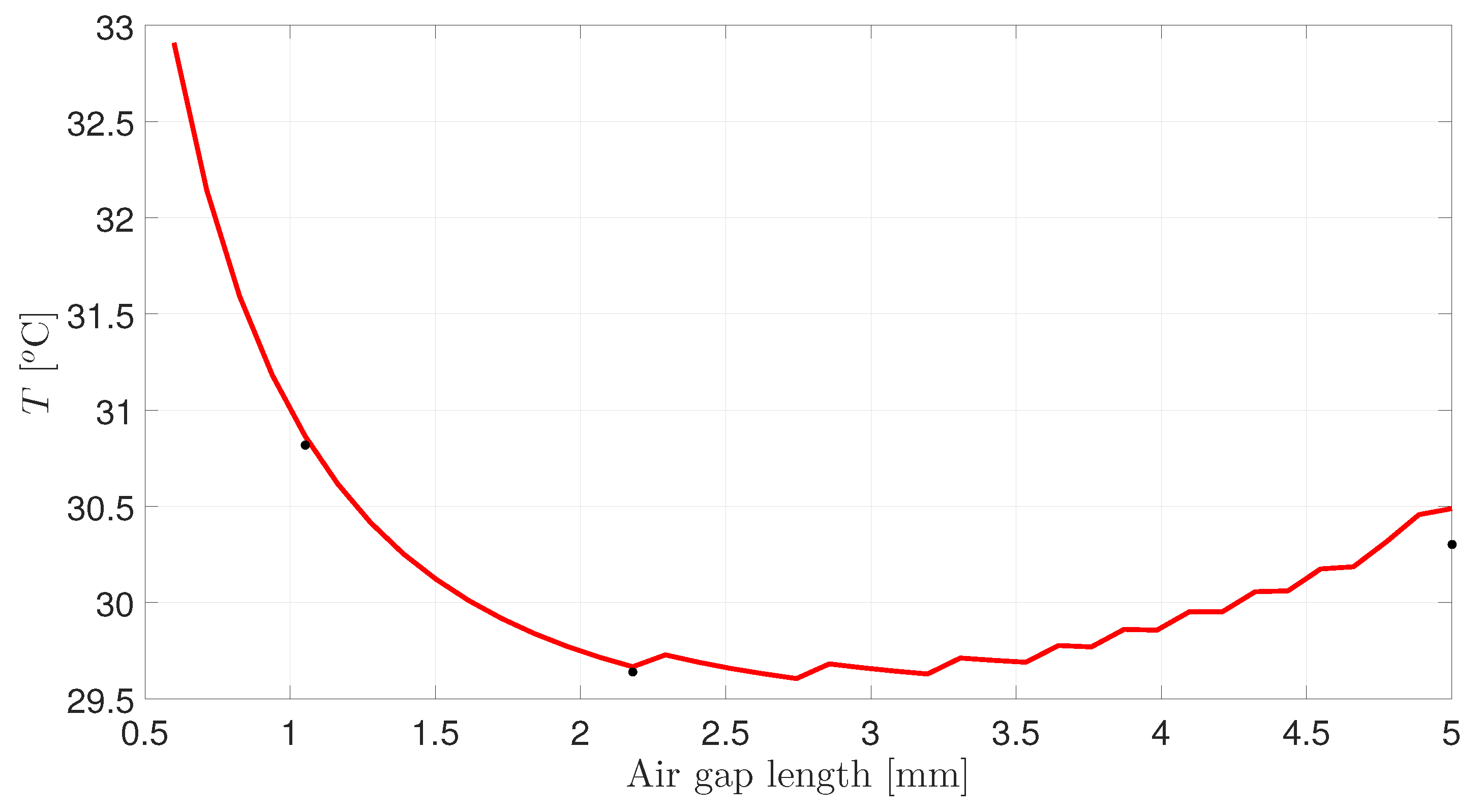
5.1. Air Gap Length Study

The study is done for air gap lengths ranging from 0.6 to 5 mm with the power and the speed fixed at 4 kW and 2500 rpm. As the air gap length increases and as the air gap flux decreases, the current needed to provide the same output torque should also increase.

The winding losses keep increasing quadratically with the air gap length as shown in Figure 6 as a result of the increasing stator current. On the other hand, the iron losses have a minimum value at 3.5 mm air gap length. This can be explained as follows: as the air gap length increases, this results in decreasing the air gap flux density component generated by the PMs and increasing the armature reaction due to increased stator current. The rate of change of the overall flux density reaches a minimum at 3.5 mm air gap length resulting in minimum core losses at this value.

The PM losses keep decreasing with the air gap length as in Figure 7.

From Figure 6, it is clear that the total losses keep increasing with the air gap length and hence, from Figure 8, the efficiency keeps decreasing from 96% at 1 mm to 84% at 5 mm.

Whether the steady-state temperature will increase or decrease with the air gap length depends not only on the losses but also on the change of the air gap convection coefficient. From Figure 9, it is seen that the air gap convection coefficient reduces with the air gap length. This explains the continuous increase in the winding and the core temperature with the air gap length as shown in Figure 10.

From Figure 11, the PM temperature has its minimum value at 2.7 mm air gap length. This can be explained by investigating Figure 7 and Figure 9. The PM losses keep decreasing which means less heat generation and also the convection coefficient keeps decreasing, which means less heat evacuation. For air gaps less than 2.7 mm, the rate by which the heat generation decreases is higher than the rate of decrease of the convection coefficient and the opposite happens at values higher than 2.7 mm.

It can also be seen that the good correspondence between the FEM results and the analytical method and the small effect of the air gap length value on the temperature of the PMs.

Based on the above presented air gap variation effects on the losses and the temperature, it is recommended to keep the air gap length as low as possible to get high operating efficiency and low temperature stresses.

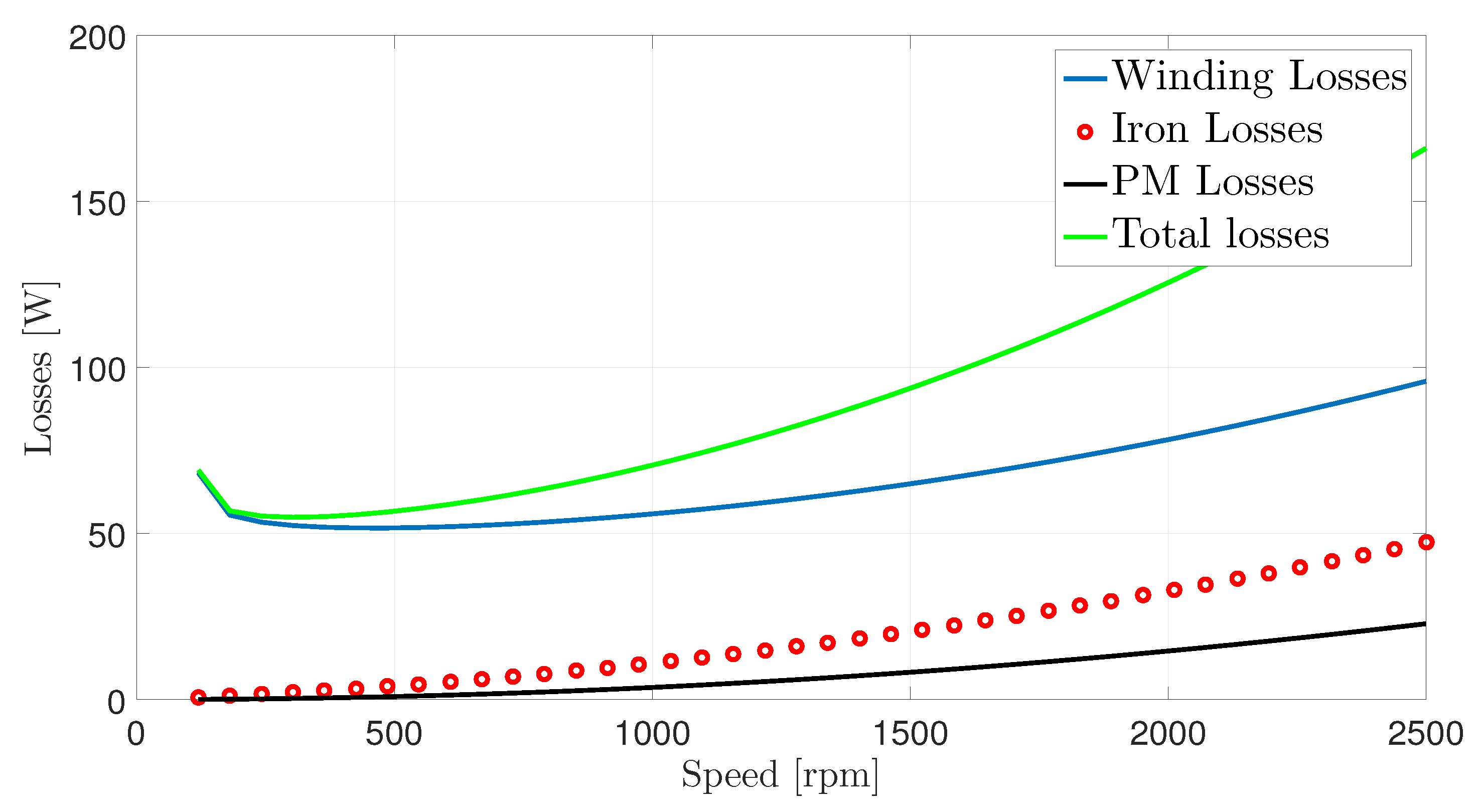
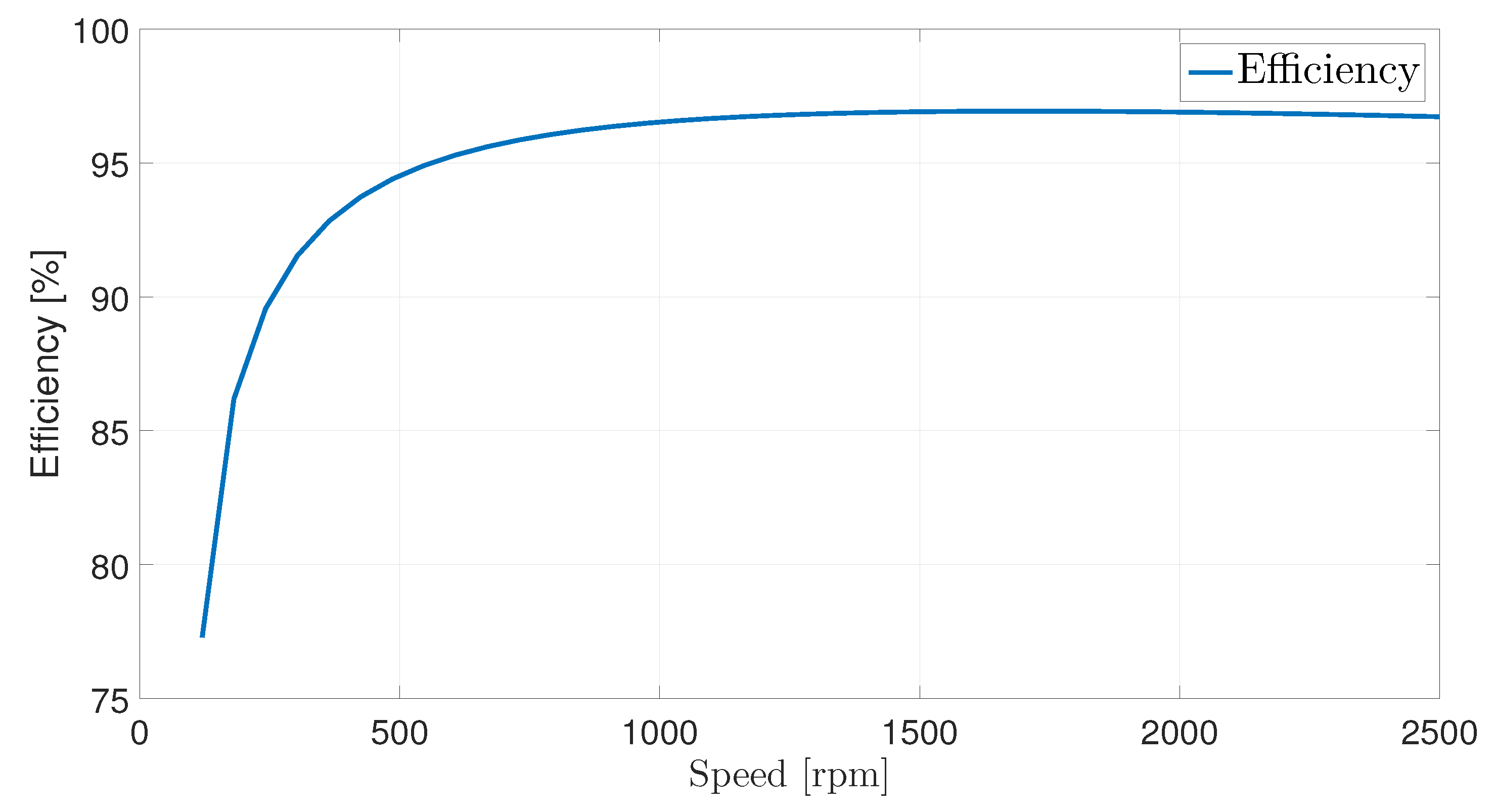
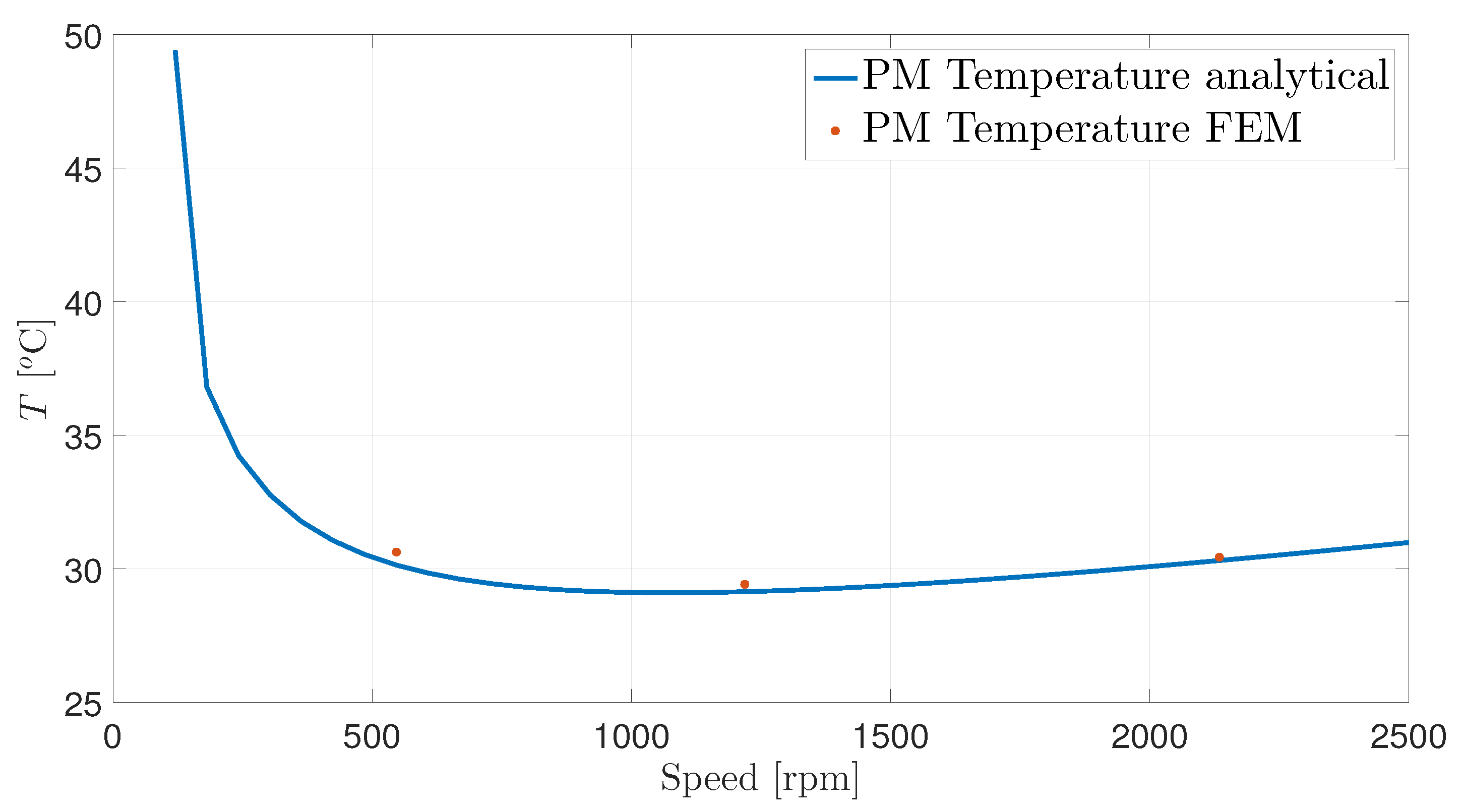
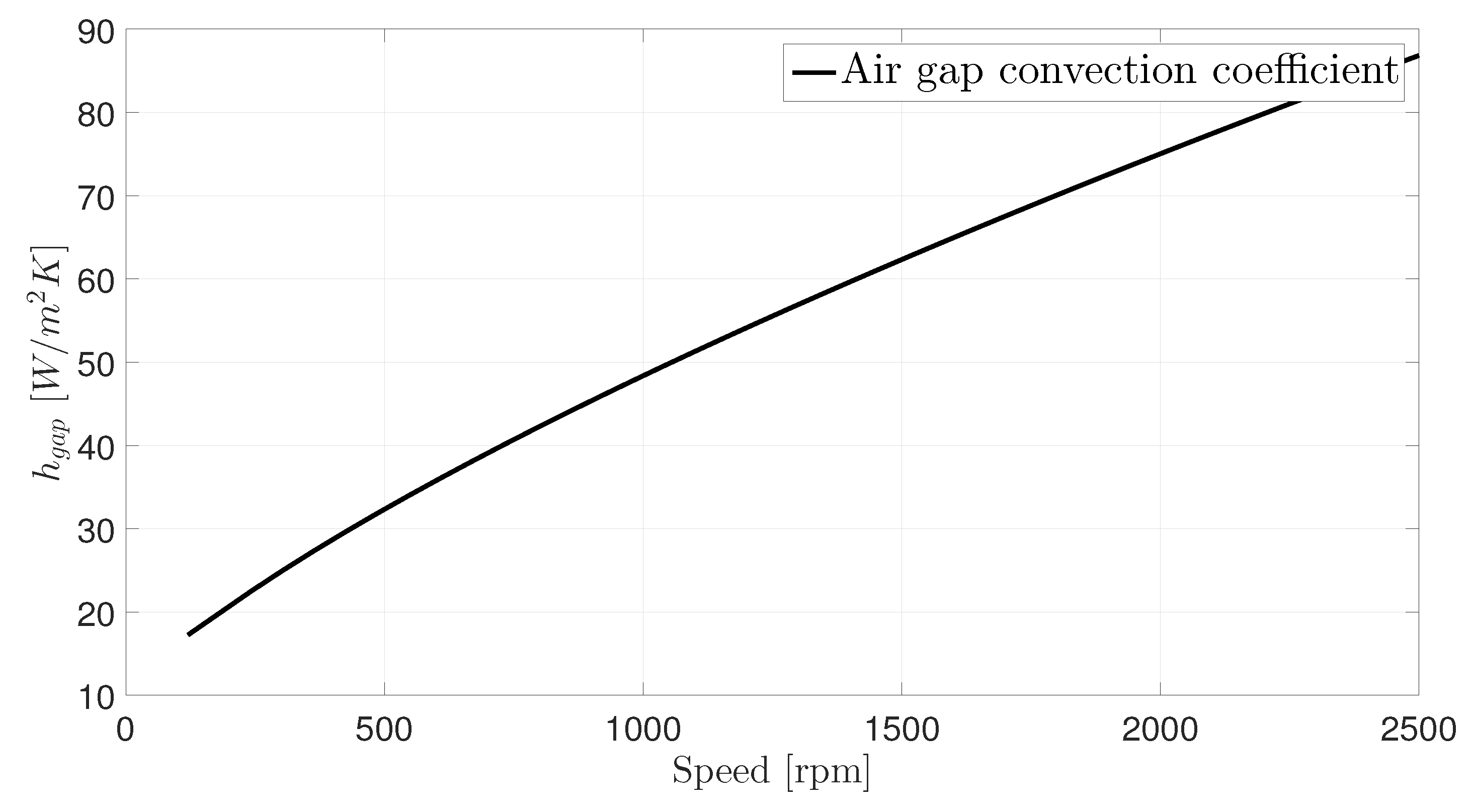
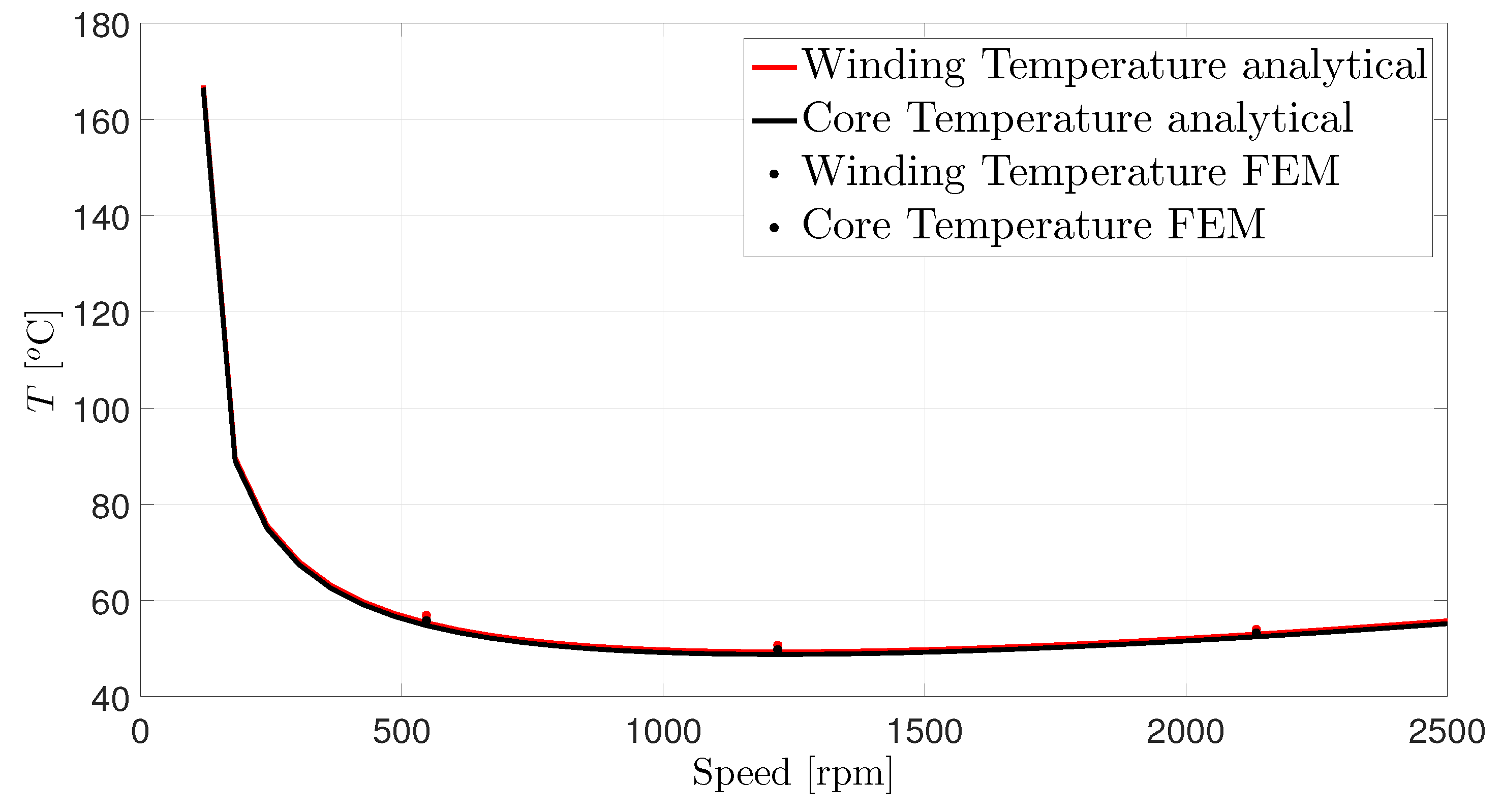
5.2. Variable Speed Study

This study is done for speed range from 120 to 2500 rpm at air gap length 1 mm and output torque fixed at 18.7 N.m, which is the rated torque of the 4 kW machine. Variable speed operation in synchronous machines requires variable supply frequency. As the supply frequency increases, the speed also increases and this results in two effects with counter actions on the machine temperature. On the one hand, the frequency increase causes an increase in all loss components in the machine, which results in higher heat generation. On the other hand, the speed increase results in higher air gap convection coefficients, which results in better heat evacuation. These counter actions make it necessary to investigate the machine temperature at different speeds to identify the safe operating speed range. From Figure 12, it can be seen that the PMs and core losses keep increasing with the speed, which is expected from Equation (1). On the other hand, the winding losses decrease in the speed range from 120 to 489 rpm.

This can be explained as follows in the low speed operation, the skin and proximity effects have a little effect on the winding resistance while, by inspecting Figure 13, the winding temperature keeps decreasing with speed up to 1218 rpm, which results in decreasing winding resistance and hence decreasing winding losses.

More investigations in Figure 12 and Figure 13 reveal that there are three regions: the first one up to speed of 486.2 rpm and explained above; the second one, from 486.2 to 1218 rpm the winding temperature still decreasing in this speed range, but the winding losses increase, which means that the skin and proximity effect became significant and resulted in an increase in the winding resistance rather than decreasing with the decreasing temperature. In the last region, the skin, the proximity and the temperature are all increasing, resulting in an increase in the winding resistance and hence the winding losses.

The efficiency variation with the speed is shown in Figure 14.

The PM temperature in Figure 15 has a minimum at a speed 1035 rpm. In the speed region below the minimum, the temperature keeps decreasing, which means that the increase in the magnet losses is lower than the increase in the convection coefficients.

It is also informative to see from Figure 16 the values of the convection coefficients at each speed value.

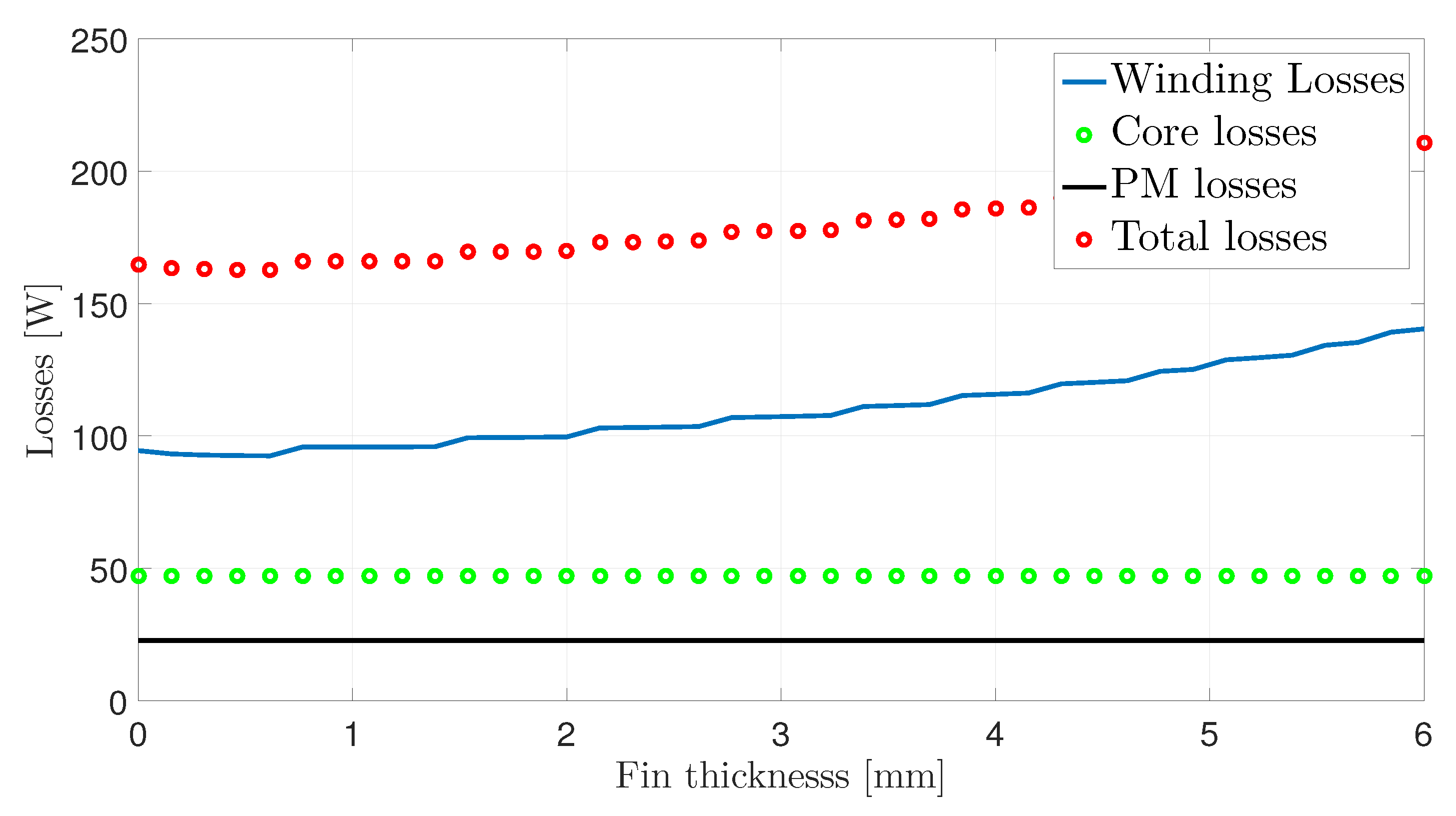
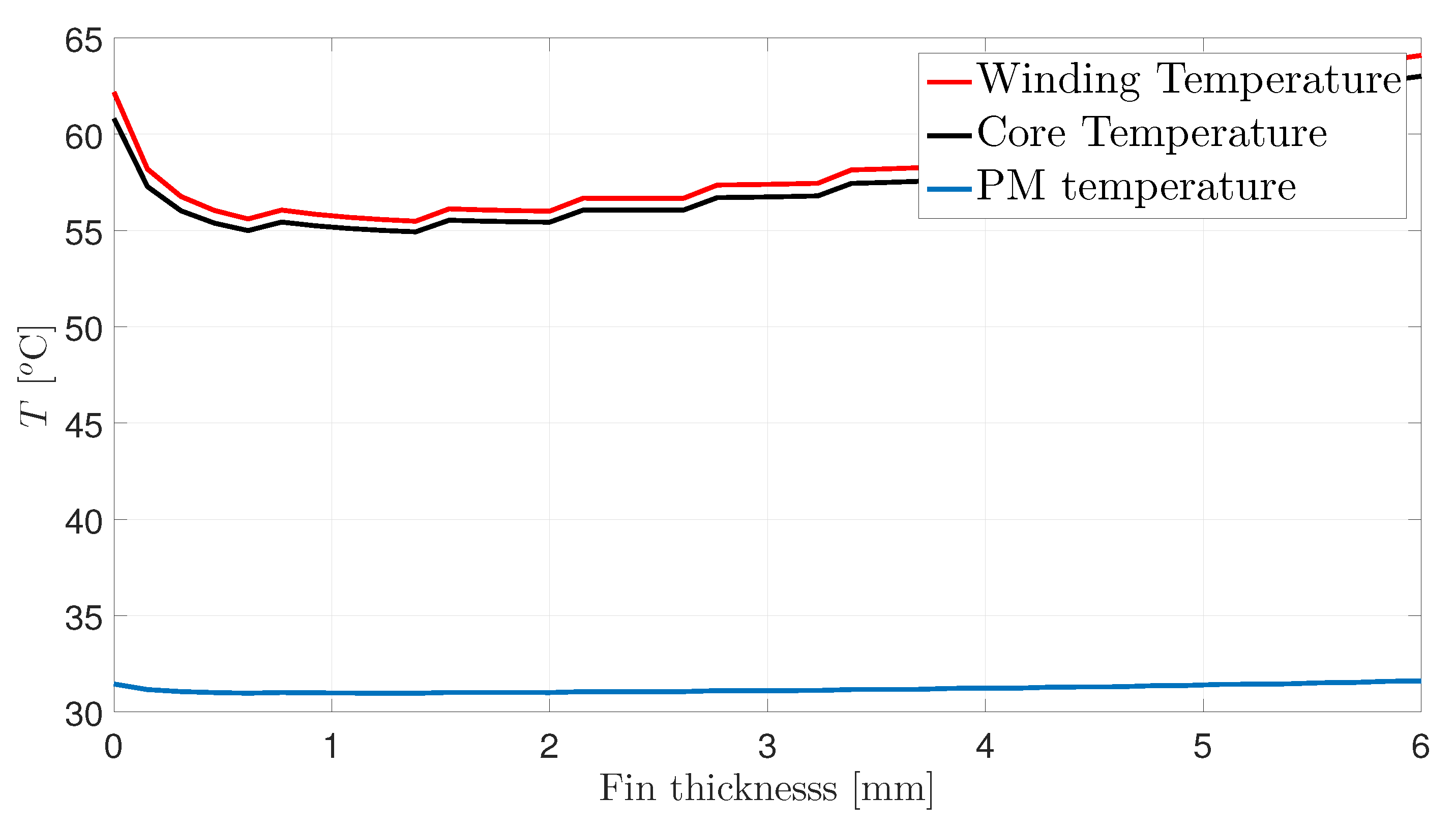
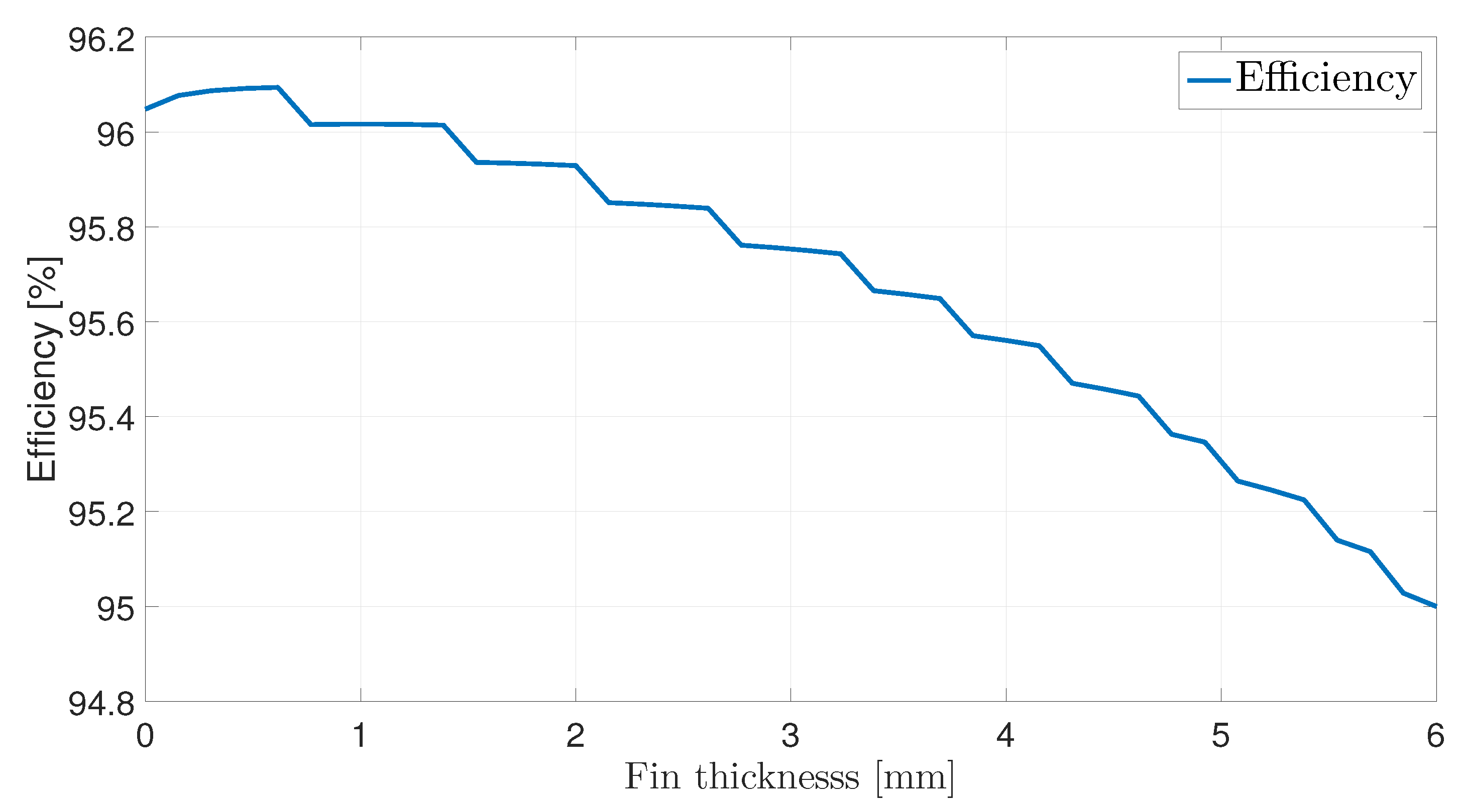
5.3. Inward Heat Extraction Fins Thickness Study

This study is done for fins thickness in the range from 0 to 6 mm at 4 kW and 2500 rpm. An inward heat extraction fins of aluminum are put between the windings to enhance the heat evacuation from the windings. Figure 17 illustrates the heat extraction fins extending along the axial length of the effective winding.

As the thickness of the inward heat extraction fins increases, its thermal resistance in the axial direction decreases. This leads to a better heat evacuation. At the same time, the slot area available for the windings will decrease, causing a lower winding factor and hence higher winding resistance and losses. Thus, the fins thickness should be selected carefully. Figure 18 shows the different losses variation with the fin thickness along with the total losses. The winding losses are minimum at 0.6 mm. This can be explained by inspecting Figure 19: the winding temperature decreases up to a thickness of 1.4 mm, which contributes to the reduction of the winding resistance and hence the winding losses. In addition, by inspecting Figure 19, the optimum fins thickness is 1.4 mm as the temperature reduces by 8 ${}^{\circ }$C compared to the case without inward heat extraction fins.

Figure 20 shows the efficiency variation with the fins thickness. It reduces from 96.1% in the case without fins to 95% at 5 mm thickness. The efficiency doesn’t decrease too much at the optimal fin thickness of 1.4 mm.

The conclusion is that the coolest machine is obtained at 1.4 mm thickness while the most efficient machine is obtained at 0.6 mm.

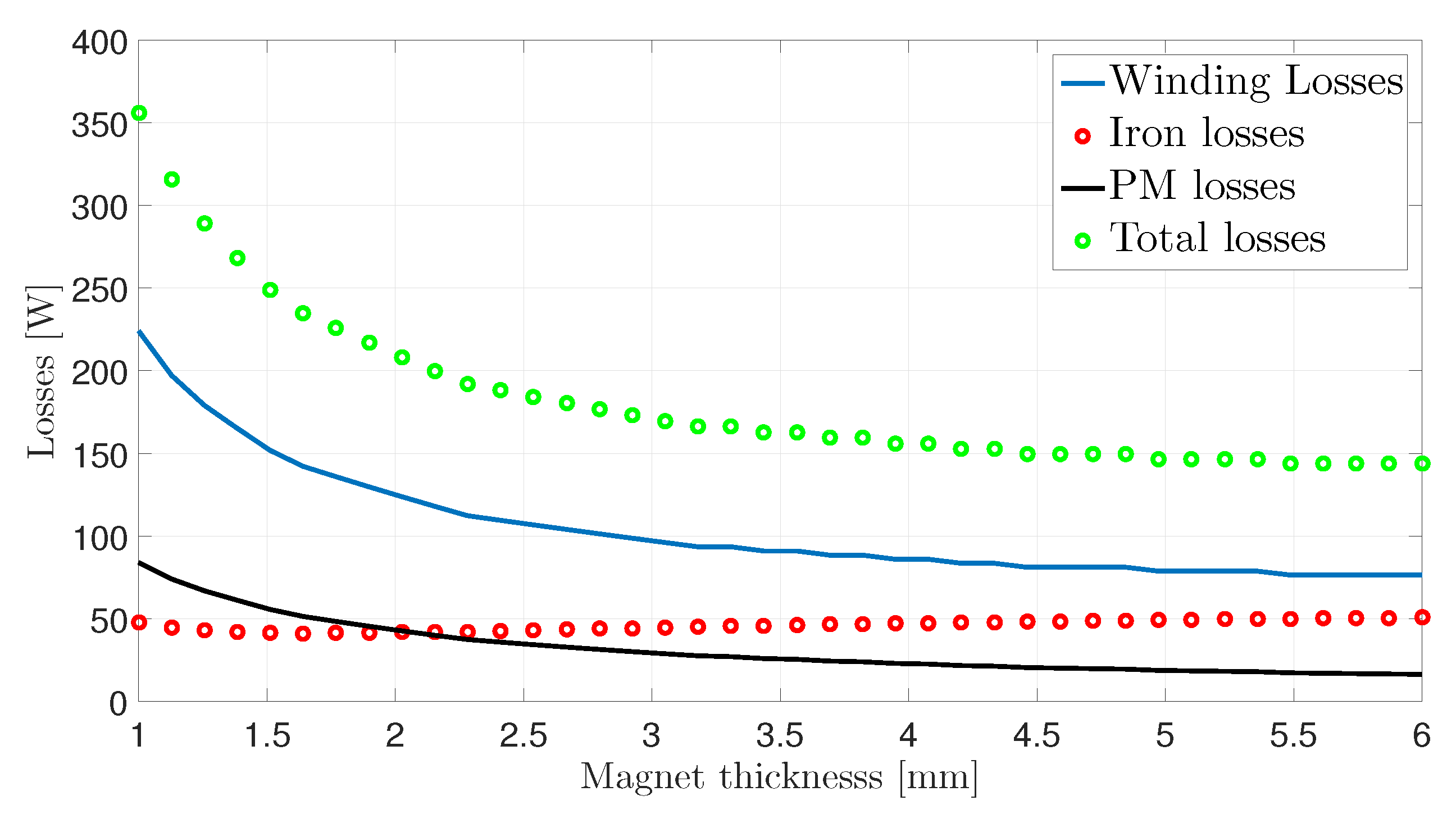
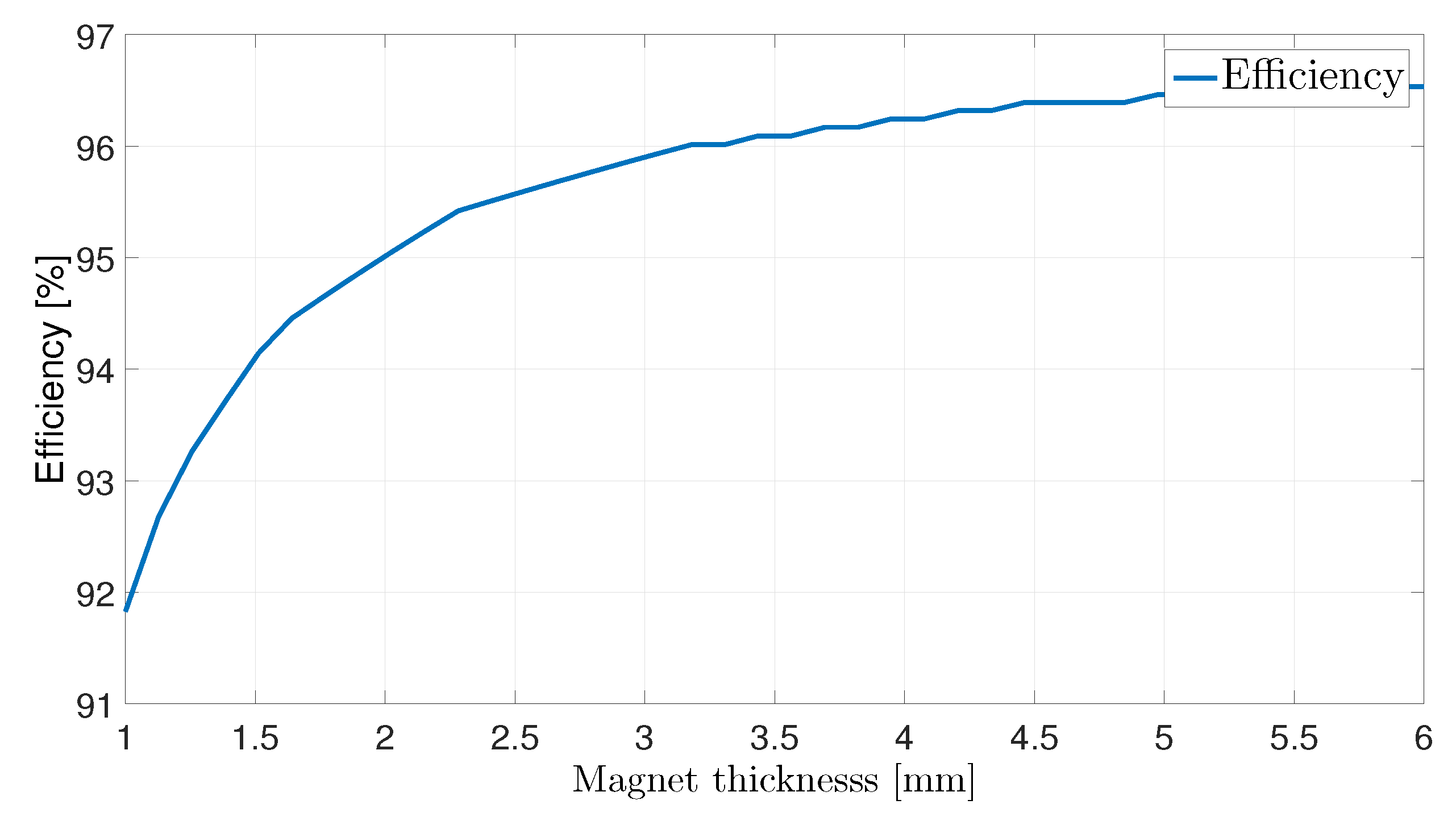
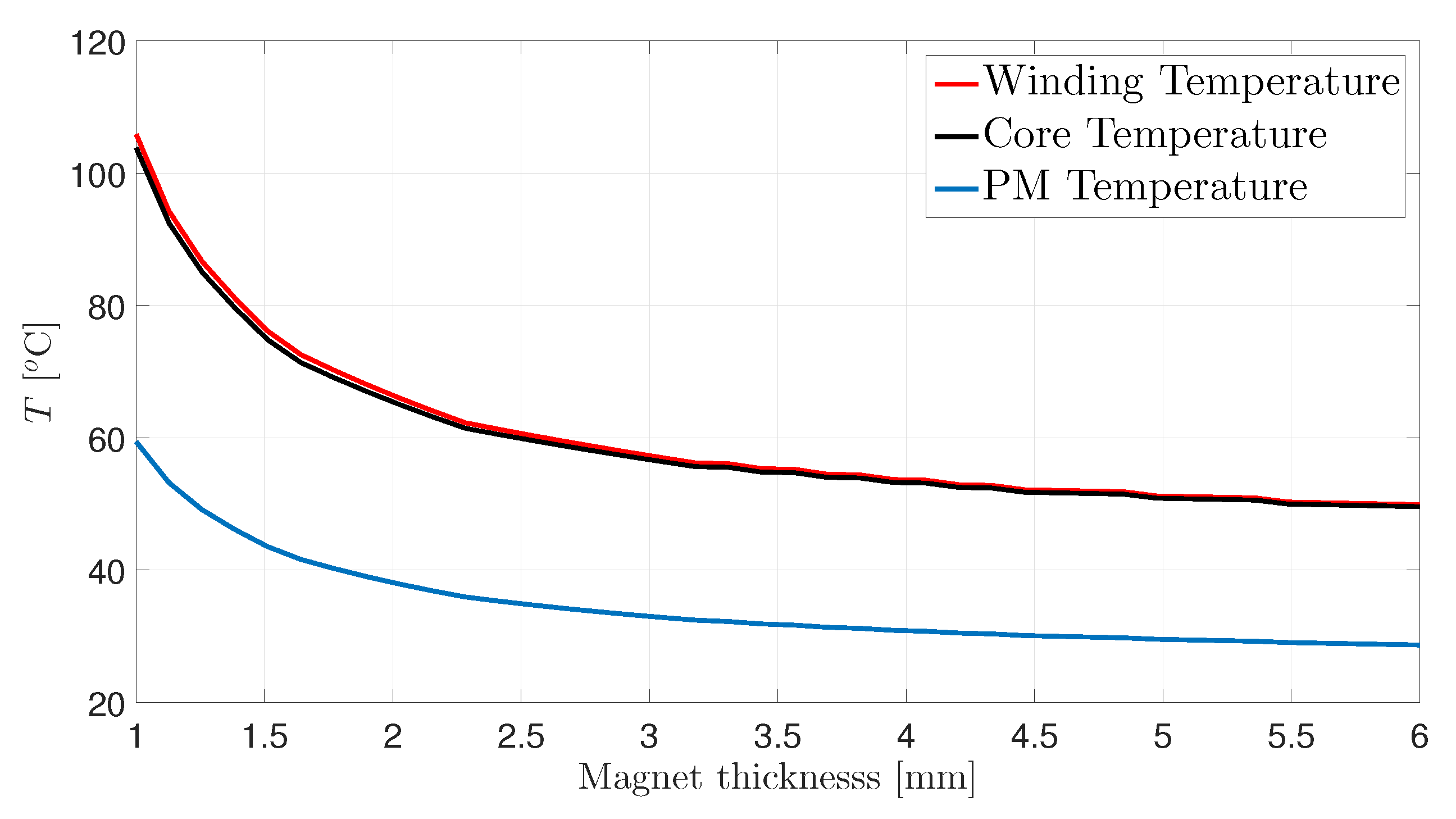
5.4. PM Thickness Study

This study is done at a magnet thickness range from 1 to 6 mm at a 4 kW and 2500 rpm. The PM thickness is one of the important parameters affecting the overall flux density in the machine and hence the losses and, at the same time, affects the air gap convection coefficient (3).

Figure 21 shows the losses variation with the magnet thickness. The copper losses keep decreasing with the magnet losses as expected, due to the decrease in the required current for getting the rated output torque at each magnet thickness. The PM losses are also decreasing with the magnet thickness. This is due to the reduction occurring in the stator current and the armature reaction. Hence, the induced voltage in the PMs will decrease, leading to a decreased PM loss.

The core losses have a minimum value at 1.6 mm magnet thickness. This can be explained by the different rate of the rise of the PM flux density and rate of decrease of the armature reaction with the PM thickness. At 1.6 mm thickness, the rate of change of the total air gap flux density hits a minimum, resulting in minimum losses.

From Figure 22, the efficiency keeps increasing with the magnet thickness.

The temperature of the three parts keeps decreasing with the magnet thickness as shown in Figure 23, which is expected from the decreasing losses.

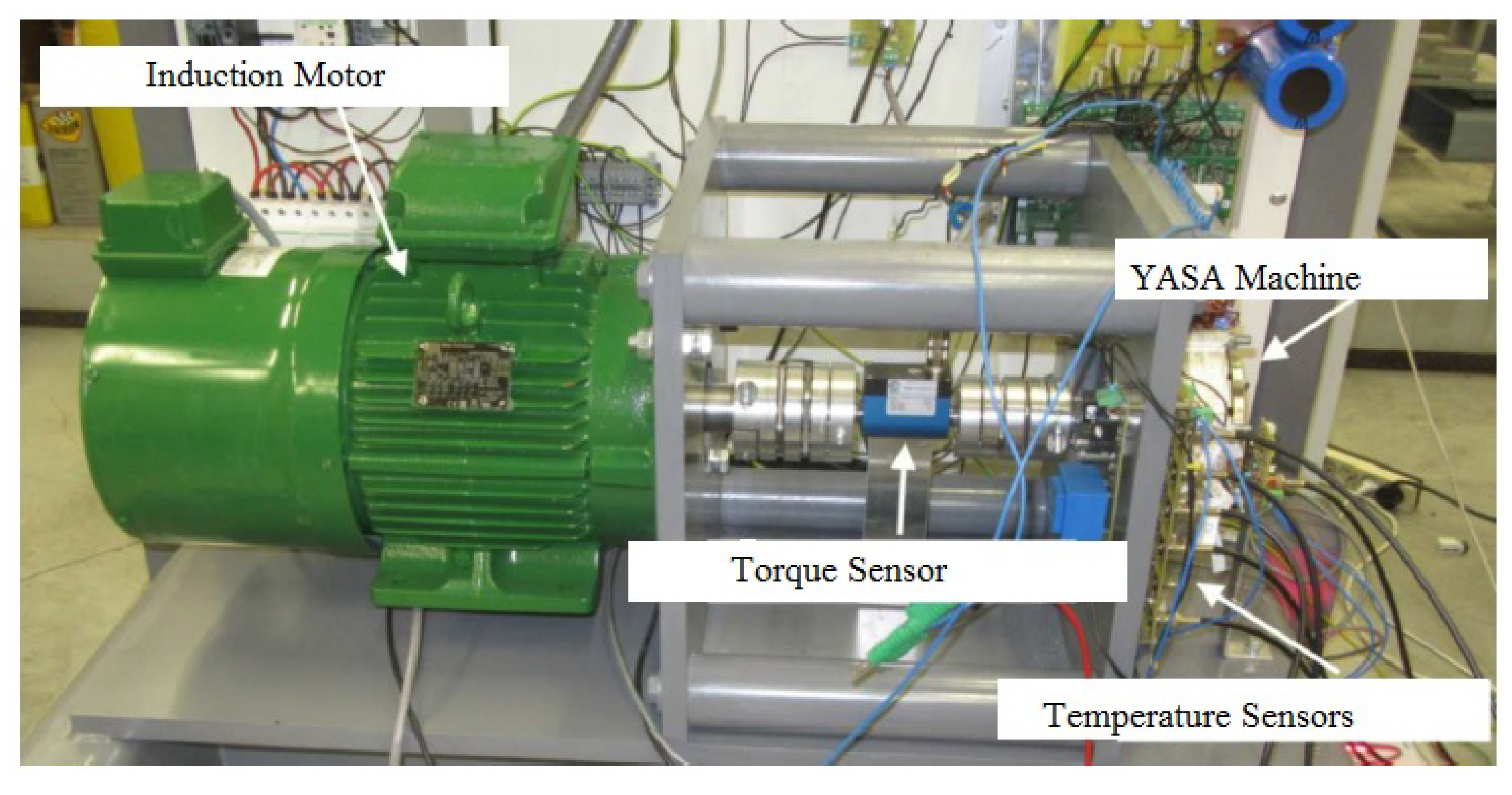
6. Experimental Validation

The validation measurements are carried out using the setup shown in Figure 24. It consists of a YASA axial flux permanent magnet synchronous machine of 4 kW and 2500 rpm rated values coupled to an induction machine of 7.5 kW and 3000 rpm rated values driven by a commercial drive. For torque measurements, a torque sensor is installed. The winding and the core temperatures are measured by an embedded resistance temperature detector (PT100) sensor, while the PM temperature is measured by an infrared temperature sensor (ZTP-135SR).

In addition, a dspace 1104 platform is used to send the speed setpoint command to the induction motor commercial drive.

To be able to precisely validate the model, all sources of uncertainties in the machine should be eliminated. To do that, the real magnets are replaced by dummy aluminum parts with the same shape and dimensions to eliminate the magnets losses. In addition, to eliminate the core losses, a DC current is injected in the stator rather than an AC one. By this method, the winding losses and the rotational losses are the only loss components remaining.

The air gap is set to 1 mm, the fins thickness is set to 1 mm and the induction motor is operated at 1000 rpm and a DC current is injected in the stator winding to get a 100 W winding losses. The temperature sensors are sampled and recorded every 5 s for 110 min. This experiment is repeated at 2000 rpm. After every experiment, the machine is completely cooled to the ambient temperature.

Table 3. Winding temperature validation.

Speed (rpm)	Analytical (${}^{\circ }$C)	FEM (${}^{\circ }$C)	Experimental (${}^{\circ }$C)
1000	61.73	63.89	62.74
2000	49.03	50.13	51.43

and

Table 4. PM temperature validation.

Speed (rpm)	Analytical (${}^{\circ }$C)	FEM (${}^{\circ }$C)	Experimental (${}^{\circ }$C)
1000	29.44	29.93	30.52
2000	26.89	27.05	28.12

are showing the winding and the PM steady state temperature at each speed value, the analytical and FEM models, and the experimental setup.

The results show a good correspondence between the models and the experimental work.

7. Conclusions

In this paper, the effect of the air gap length, the speed, the inward heat extraction fins thickness and the PM thickness on the different power losses and the temperature of the different components are studied at the rated load condition. The skin and proximity effects are taken into account and the temperature dependent electrical conductivities are also taken into account in these coupled electromagnetic-thermal studies. The results reveal that the winding and core temperature are much more sensitive to the changes in the air gap length, the speed and the inward heat extraction fins than the PM temperature. In all these studies, the temperature variation with the variable under study can be divided into regions. In every region, one of the factors affecting the increase or the decrease in the temperature dominates over the others. Based on these studies, the recommended air gap range is determined, the safe operating speed range is identified and the optimum inward heat extraction fins thickness is revealed.

References

1. Giulii Capponi, F.; De Donato, G.; Caricchi, F. Recent advances in axial-flux permanent-magnet machine technology. IEEE Trans. Ind. Appl. 2012, 48, 2190–2205. [Google Scholar] [CrossRef]
2. Hemeida, A.; Sergeant, P. Analytical modeling of surface PMSM using a combined solution of Maxwell’s equations and Magnetic Equivalent Circuit (MEC). IEEE Trans. Magn. 2014, 50, 7027913. [Google Scholar] [CrossRef]
3. Woolmer, T.J.; McCulloch, M.D. Analysis of the yokeless and segmented armature machine. In Proceedings of the IEEE International Electric Machines and Drives Conference, IEMDC 2007, Antalya, Turkey, 3–5 May 2007; Volume 1, pp. 704–708. [Google Scholar]
4. Letelier, A.B.; González, D.A.; Tapia, J.J.A.; Wallace, R.; Valenzuela, M.A. Cogging torque reduction in an axial flux PM machine via stator slot displacement and skewing. IEEE Trans. Ind. Appl. 2007, 43, 685–693. [Google Scholar] [CrossRef]
5. Wang, Z.; Masaki, R.; Morinaga, S.; Enomoto, Y.; Itabashi, H.; Ito, M.; Tanigawa, S. Development of an axial gap motor with amorphous metal cores. IEEE Trans. Ind. Appl. 2011, 47, 1293–1299. [Google Scholar] [CrossRef]
6. Hemeida, A.; Sergeant, P.; Vansompel, H. Comparison of Methods for Permanent Magnet Eddy Current Loss Computations With and Without Reaction Field Considerations in Axial Flux PMSM. IEEE Trans. Magn. 2015, 9464, 1–11. [Google Scholar] [CrossRef]
7. Hsieh, M.F.; Hsu, Y.C. A Generalized Magnetic Circuit Modeling Approach for Design of Surface Permanent-Magnet Machines. IEEE Trans. Ind. Electron. 2012, 59, 779–792. [Google Scholar] [CrossRef]
8. Kano, Y.; Kosaka, T.; Matsui, N. A simple nonlinear magnetic analysis for axial-flux permanent-magnet machines. IEEE Trans. Ind. Electron. 2010, 57, 2124–2133. [Google Scholar] [CrossRef]
9. Tangudu, J.; Jahns, T.; EL-Refaie, A.; Zhu, Z. Lumped parameter magnetic circuit model for fractional-slot concentrated-winding interior permanent magnet machines. In Proceedings of the 2009 IEEE Energy Conversion Congress and Exposition, San Jose, CA, USA, 20–24 September 2009; pp. 2423–2430. [Google Scholar]
10. Tan, Z.; Song, X.G.; Ji, B.; Liu, Z.; Ma, J.E.; Cao, W.P. 3D thermal analysis of a permanent magnet motor with cooling fans. J. Zhejiang Univ. Sci. A 2015, 16, 616–621. [Google Scholar] [CrossRef]
11. Polikarpova, M.; Ponomarev, P.; Lindh, P.; Petrov, I.; Jara, W.; Naumanen, V.; Tapia, J.A.; Pyrhonen, J. Hybrid Cooling Method of Axial-Flux Permanent-Magnet Machines for Vehicle Applications. IEEE Trans. Ind. Electron. 2015, 62, 7382–7390. [Google Scholar] [CrossRef]
12. Marignetti, F.; Delli Colli, V.; Coia, Y. Design of Axial Flux PM Synchronous Machines Through 3-D Coupled Electromagnetic Thermal and Fluid-Dynamical Finite-Element Analysis. IEEE Trans. Ind. Electron. 2008, 55, 3591–3601. [Google Scholar] [CrossRef]
13. Marignetti, F.; Colli, V. Thermal Analysis of an Axial Flux Permanent-Magnet Synchronous Machine. IEEE Trans. Magn. 2009, 45, 2970–2975. [Google Scholar] [CrossRef]
14. Rostami, N.; Feyzi, M.R.; Pyrhonen, J.; Parviainen, A.; Niemela, M. Lumped-Parameter Thermal Model for Axial Flux Permanent Magnet Machines. IEEE Trans. Magn. 2013, 49, 1178–1184. [Google Scholar] [CrossRef]
15. Lim, C.; Bumby, J.; Dominy, R.; Ingram, G.; Mahkamov, K.; Brown, N.; Mebarki, A.; Shanel, M. 2-D lumped-parameter thermal modelling of axial flux permanent magnet generators. In Proceedings of the 2008 18th International Conference on Electrical Machines, Vilamoura, Portugal, 6–9 September 2008; pp. 1–6. [Google Scholar]
16. Mohamed, A.H.; Hemeida, A.; Rashekh, A.; Vansompel, H.; Arkkio, A.; Sergeant, P. A 3D Dynamic Lumped Parameter Thermal Network of Air-Cooled YASA Axial Flux Permanent Magnet Synchronous Machine. Energies 2018, 11, 774. [Google Scholar] [CrossRef]
17. Jiang, W.; Member, S.; Jahns, T.M. Coupled Electromagnetic-Thermal Analysis of Electric Machines Including Transient Operation Based on Finite-Element Techniques. IEEE Trans. Ind. Appl. 2015, 51, 1880–1889. [Google Scholar] [CrossRef]
18. Bertotti, G. General Properties of Power Losses in Soft Ferromagnetic Materials. IEEE Trans. Magn. 1987, 24, 621–630. [Google Scholar] [CrossRef]
19. Vansompel, H. Design of an Energy Efficient Axial Flux Permanent Magnet Machine. Ph.D. thesis, Ghent University, Ghent, Belgium, 2013. [Google Scholar]
20. Rasekh, A.; Sergeant, P.; Vierendeels, J. Convective heat transfer prediction in disk-type electrical machines. Appl. Therm. Eng. 2015, 91, 778–790. [Google Scholar] [CrossRef]
21. Rasekh, A.; Sergeant, P.; Vierendeels, J. Fully predictive heat transfer coefficient modeling of an axial flux permanent magnet synchronous machine with geometrical parameters of the magnets. Appl. Therm. Eng. 2017, 110, 1343–1357. [Google Scholar] [CrossRef]
Figure 1. Cross-section view of the YASA prototype.
Energies 11 02983 g001
Figure 2. LPTN of the stator.
Energies 11 02983 g002
Figure 3. LPTN of the rotor.
Energies 11 02983 g003
Figure 4. Machine Modeled parts (a) Stator modeled part: (1) thermal insulation; (2) stator facing rotor upper part; (3) stator facing rotor lower part; (4) stator side wall. (b) Rotor modeled part: (8) rotor facing stator upper; (9) rotor left side; (10) PM lower; (11) rotor lower; (12) PM upper; (13) rotor upper; (14) PM left; (15) PM right; (16) rotor facing stator.
Energies 11 02983 g004
Figure 5. The calculations flow chart.
Energies 11 02983 g005
Figure 6. The winding and the total losses variation with the air gap length.
Energies 11 02983 g006
Figure 7. The core and the PM losses variation with the air gap length.
Energies 11 02983 g007
Figure 8. The efficiency variation with the air gap length.
Energies 11 02983 g008
Figure 9. The air gap convection coefficient variation with the air gap length.
Energies 11 02983 g009
Figure 10. The winding and the core temperature variation with the air gap length.
Energies 11 02983 g010
Figure 11. The PM temperature variation with the air gap length.
Energies 11 02983 g011
Figure 12. The winding, core, PMs and total loss variation with the speed.
Energies 11 02983 g012
Figure 13. The winding and the core temperature variation with the speed.
Energies 11 02983 g013
Figure 14. The efficiency variation with the speed.
Energies 11 02983 g014
Figure 15. The PM temperature variation with the speed.
Energies 11 02983 g015
Figure 16. The air gap convection coefficient variation with the speed.
Energies 11 02983 g016
Figure 17. A quarter tooth part illustrating the inward heat extraction fins.
Energies 11 02983 g017
Figure 18. The losses variation with the fins thickness.
Energies 11 02983 g018
Figure 19. The winding, the core and the PM temperature variation with the fins thickness.
Energies 11 02983 g019
Figure 20. The efficiency variation with the fins thickness.
Energies 11 02983 g020
Figure 21. The losses variation with the magnet thickness.
Energies 11 02983 g021
Figure 22. The efficiency variation with the magnet thickness.
Energies 11 02983 g022
Figure 23. The temperature variation with the magnet thickness.
Energies 11 02983 g023
Figure 24. The experimental setup.
Energies 11 02983 g024