A CVaR-Robust Risk Aversion Scheduling Model for Virtual Power Plants Connected with Wind-Photovoltaic-Hydropower-Energy Storage Systems, Conventional Gas Turbines and Incentive-Based Demand Responses

Abstract
:1. Introduction
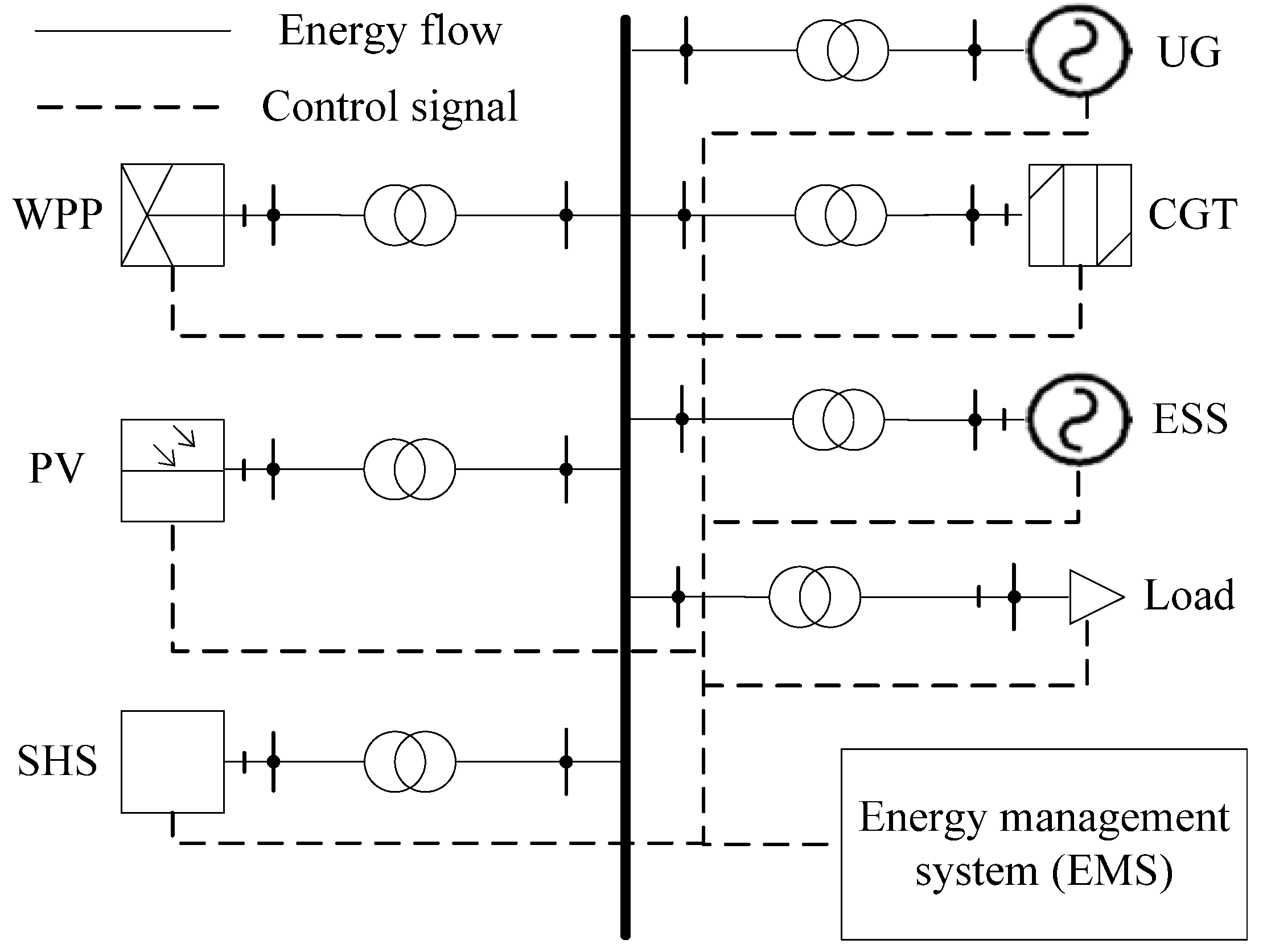
- A VPP coupled with WPP, PV, SHS, ESS, CGT, and an incentive-based demand response (IBDR) with the implementation of PBDR on the user side. Among these, the SHS equipped with regulating reservoirs can distribute the output according to the real-time load demand, which can provide reserve services for the WPP and PV coupling operation with CGT and ESS. WPP and PV have high environmental and economic benefits, as well as high risks, so balancing the benefits and risks is the key to the optimal operation of the VPP.
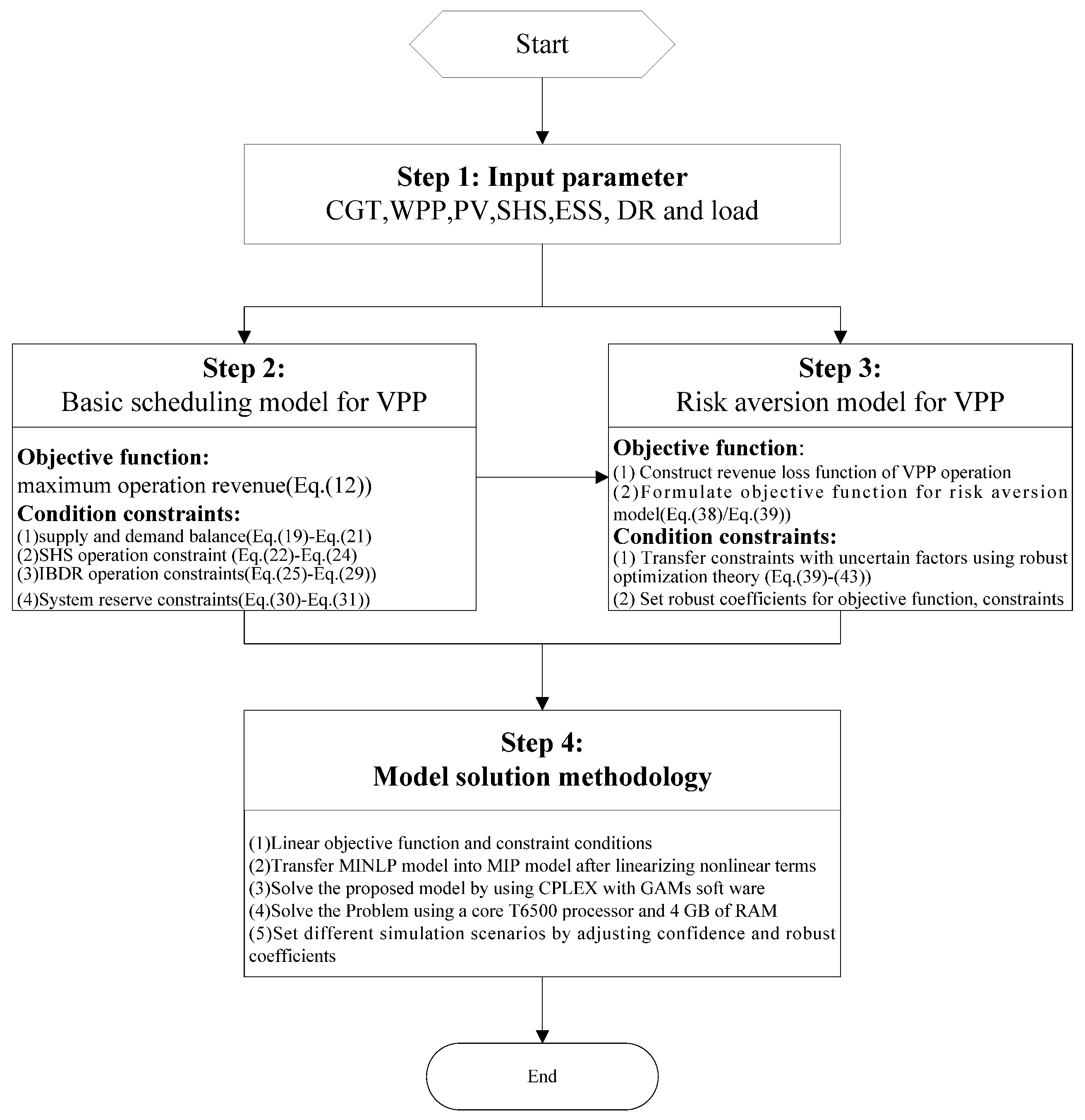
- A basic scheduling model for the VPP operation is put forward without considering uncertainty. The maximum revenue of the VPP operation is taken as the objective function of the optimization model, considering energy balance constraints, different power sources, and system rotating reserve constraints. The basic scheduling results could provide an important decision-making reference for determining the VPP operation risks and verifying the effectiveness of the risk aversion model.
- A CVaR-robust-based aversion scheduling model for the VPP operation is constructed with the objective function of minimum operation losses. First, the uncertainty analysis for WPP, PV, SHS, and the load are made, and WPP and PV selected as the main uncertainty factors. Second, the conditional value at risk (CVaR) method and robust optimization theory are used to reflect the operation risks brought about by uncertainty in the objective function and restrictions, respectively. Finally, a solution methodology is constructed after converting the mixed integer nonlinear programming (MINLP) model into a mixed integer linear programming (MIP) model with three cases for comparative analysis.
2. VPP Description
2.1. VPP Participants
2.2. VPP Output Model
3. Basic Scheduling Model for VPP
3.1. Objective Function
3.2. Constraint Conditions
4. Risk Aversion Model for VPP
4.1. Uncertainty Analysis
4.2. Mathematical Model
4.2.1. CVaR Theory
4.2.2. CVaR-Robust Model
4.3. Solution Methodology
5. Case Analysis
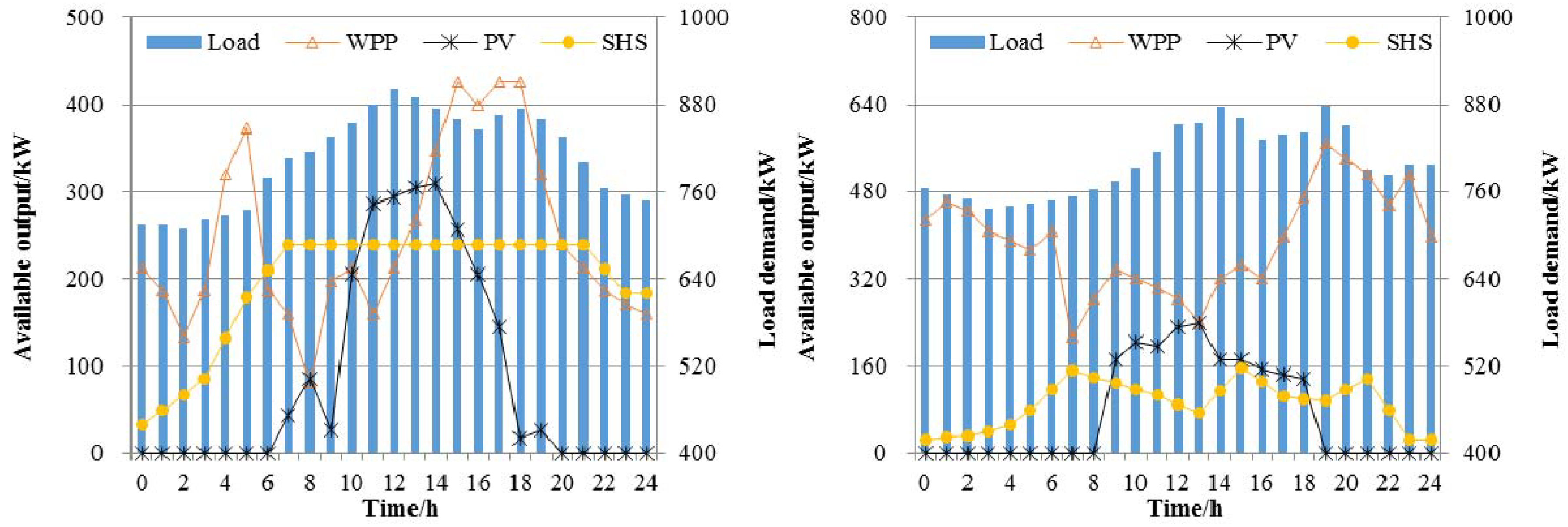
5.1. Basic Data
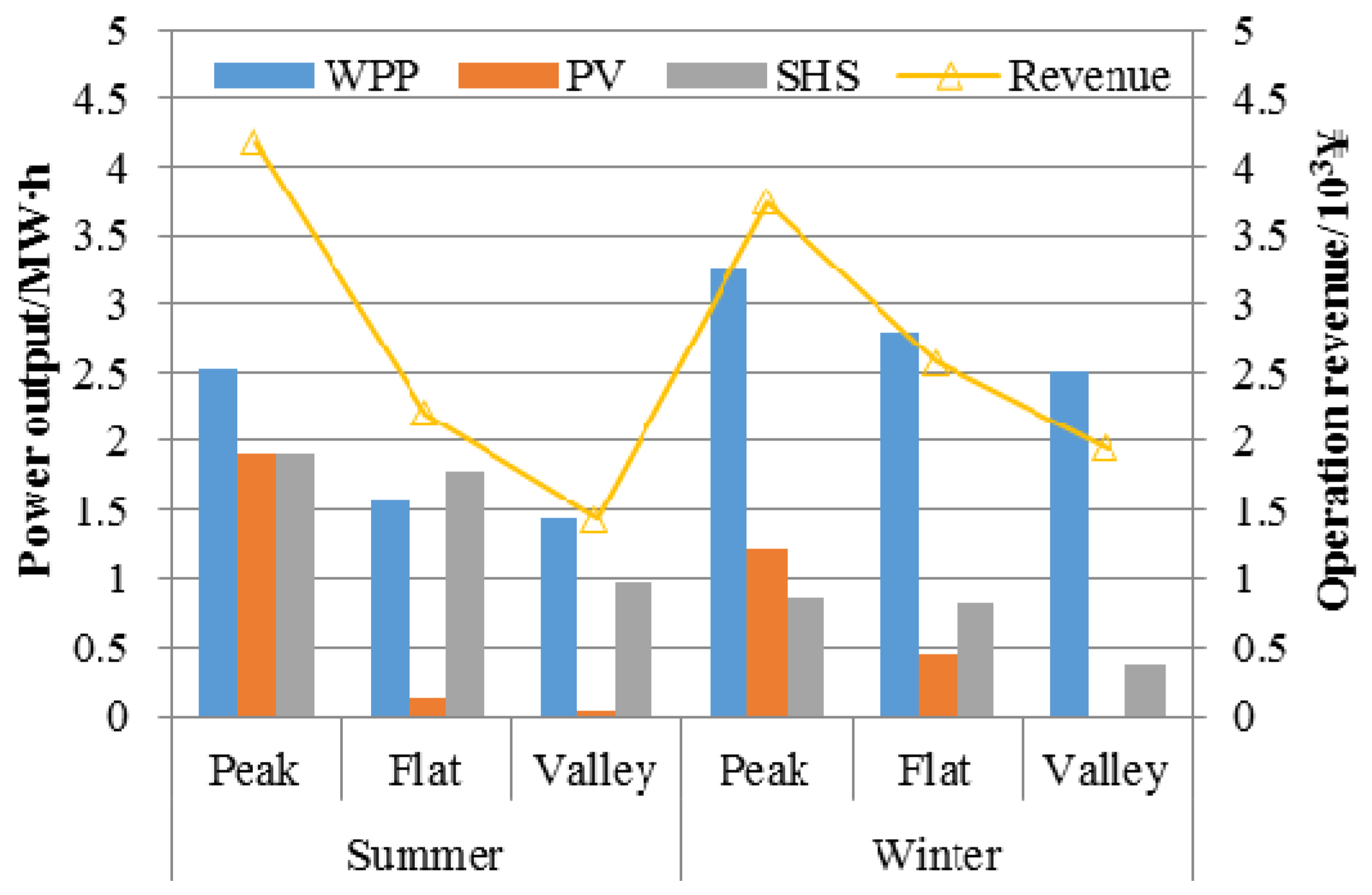
5.2. Result Analysis
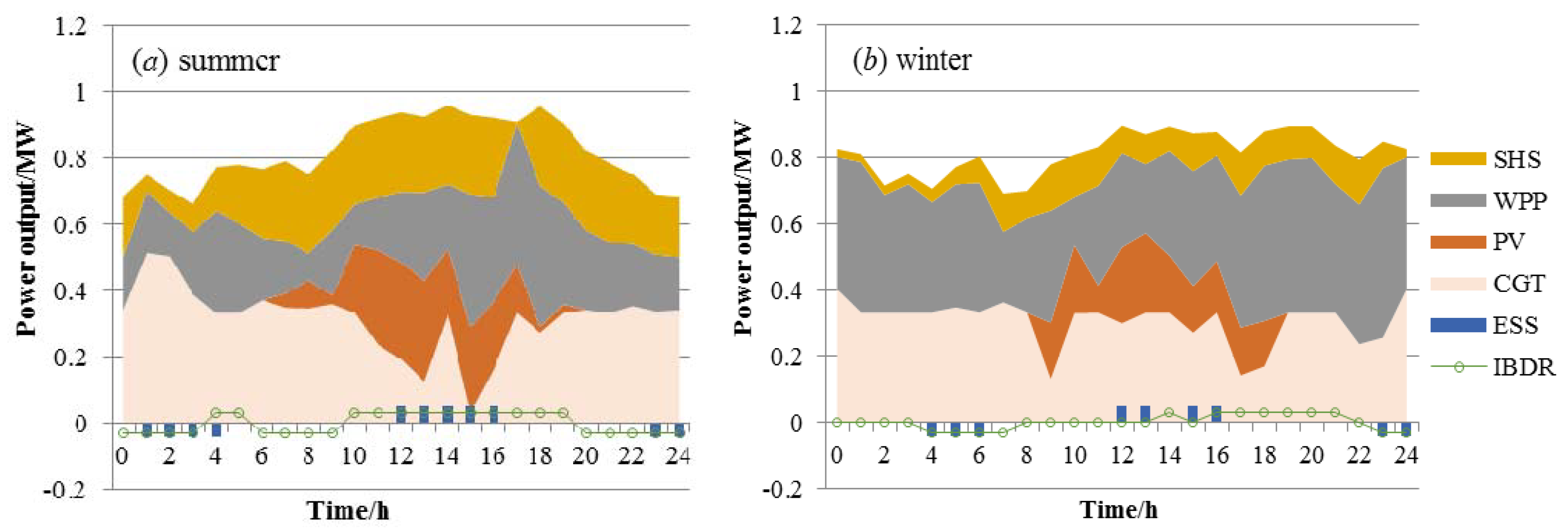
5.2.1. Scheduling Result of VPP in Case 1
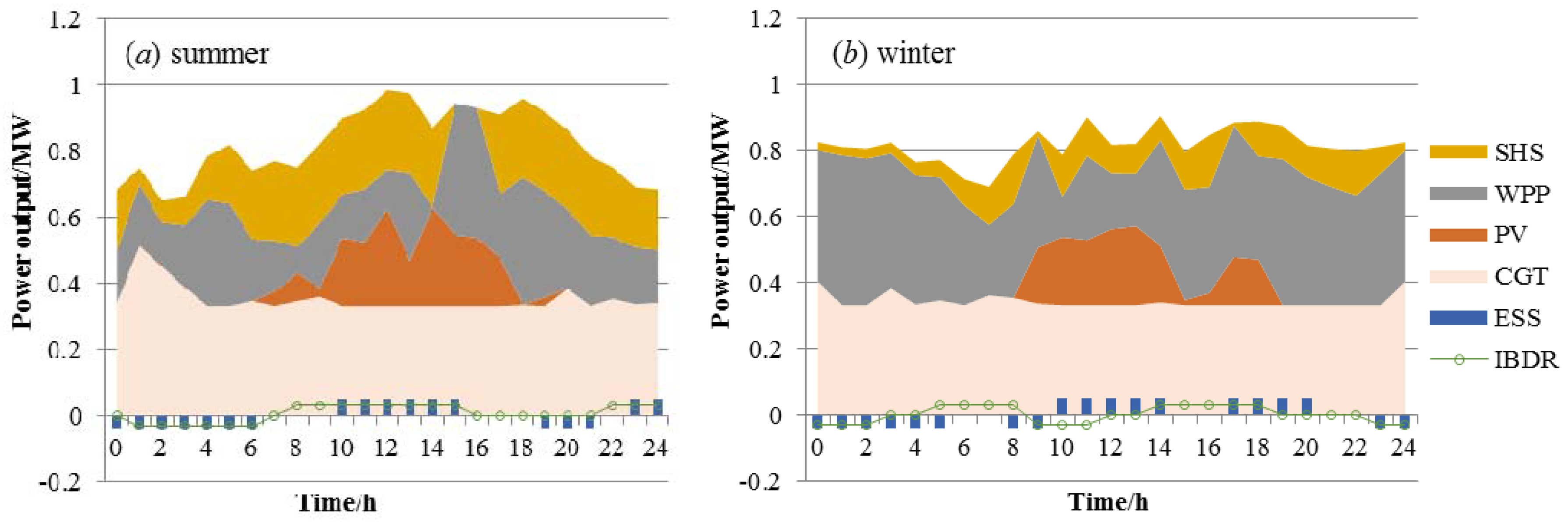
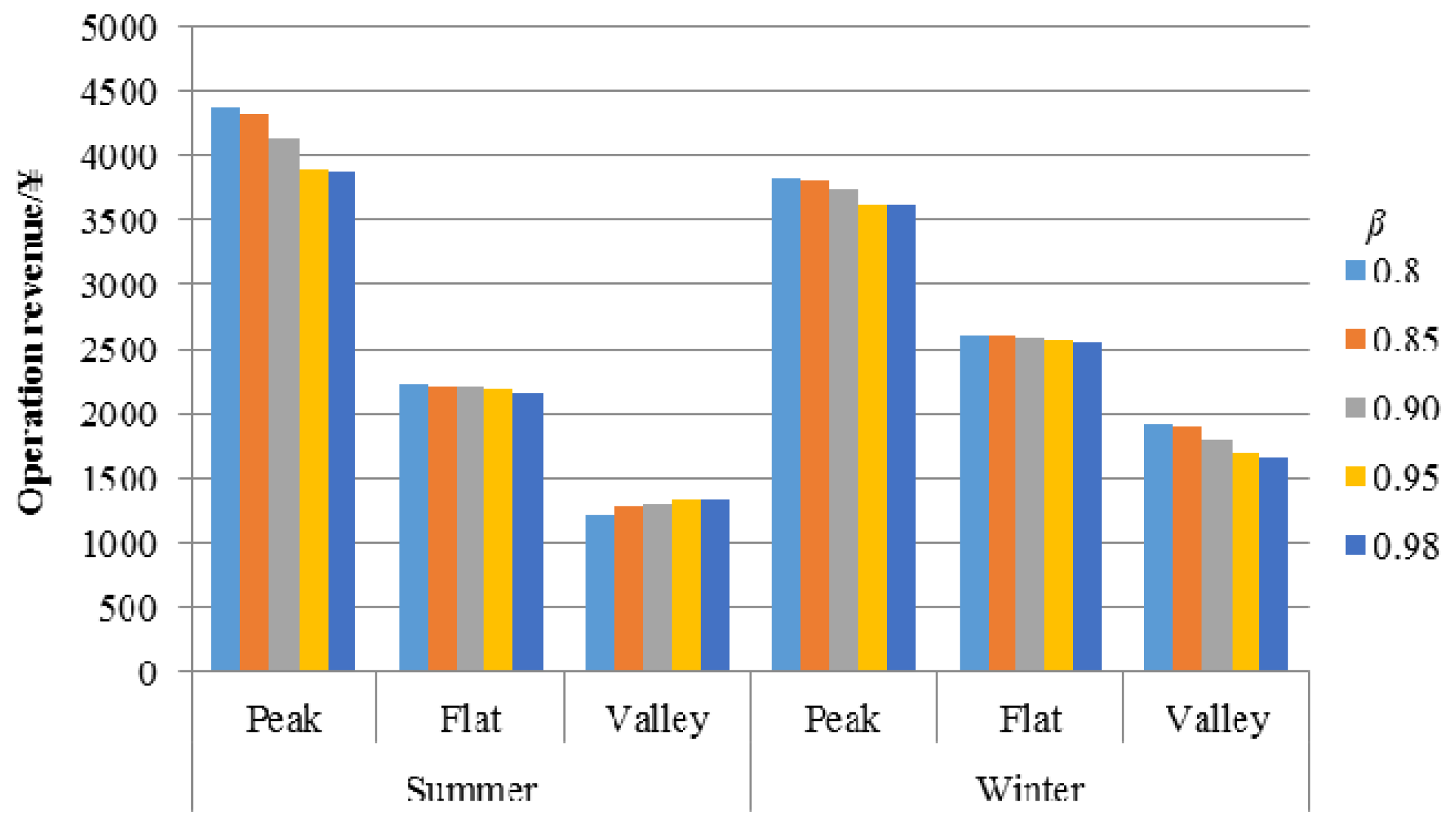
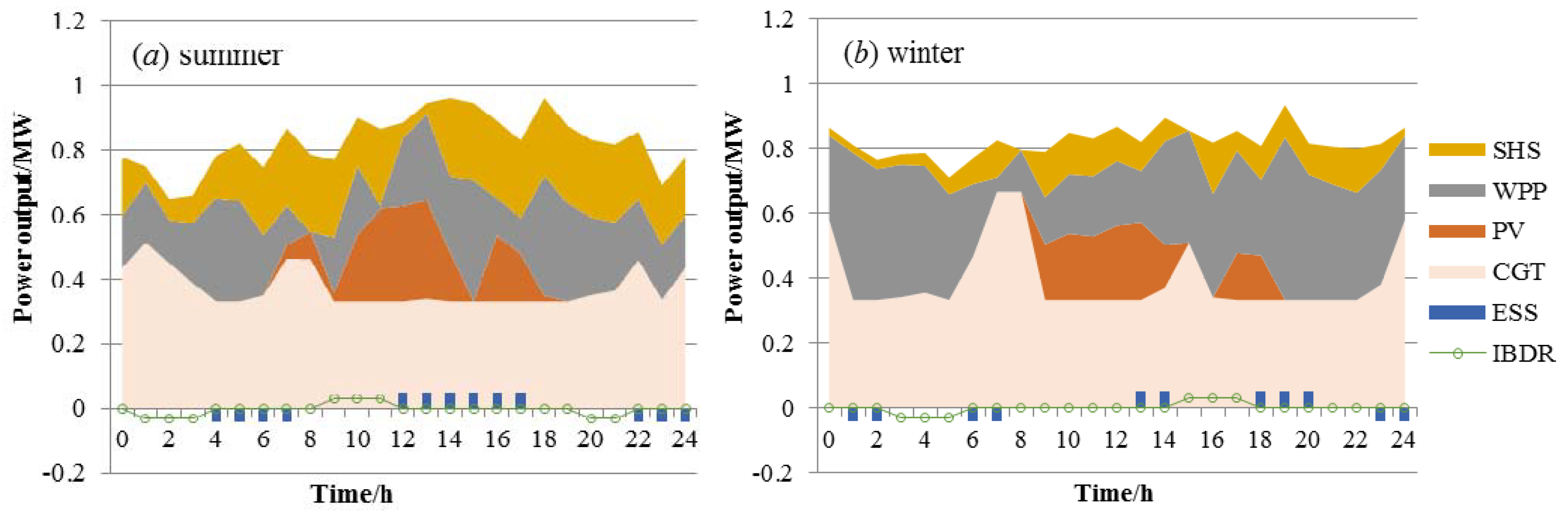
5.2.2. Scheduling Result of VPP in Case 2
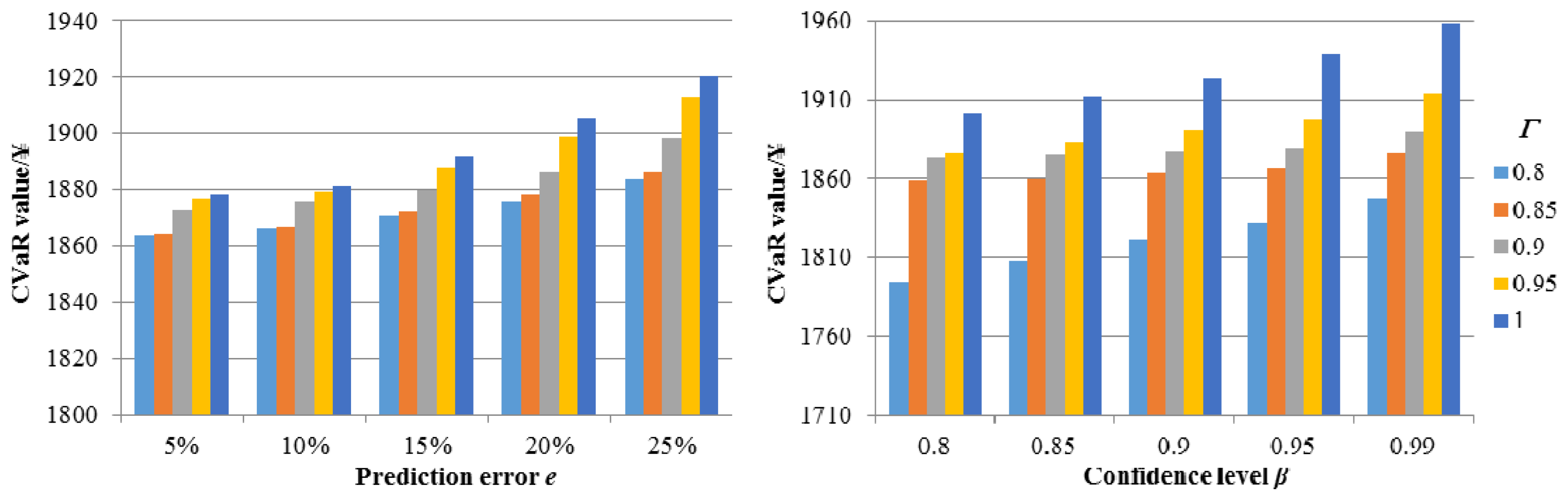
5.2.3. Scheduling Result of VPP in Case 3
5.3. Comparative Analysis
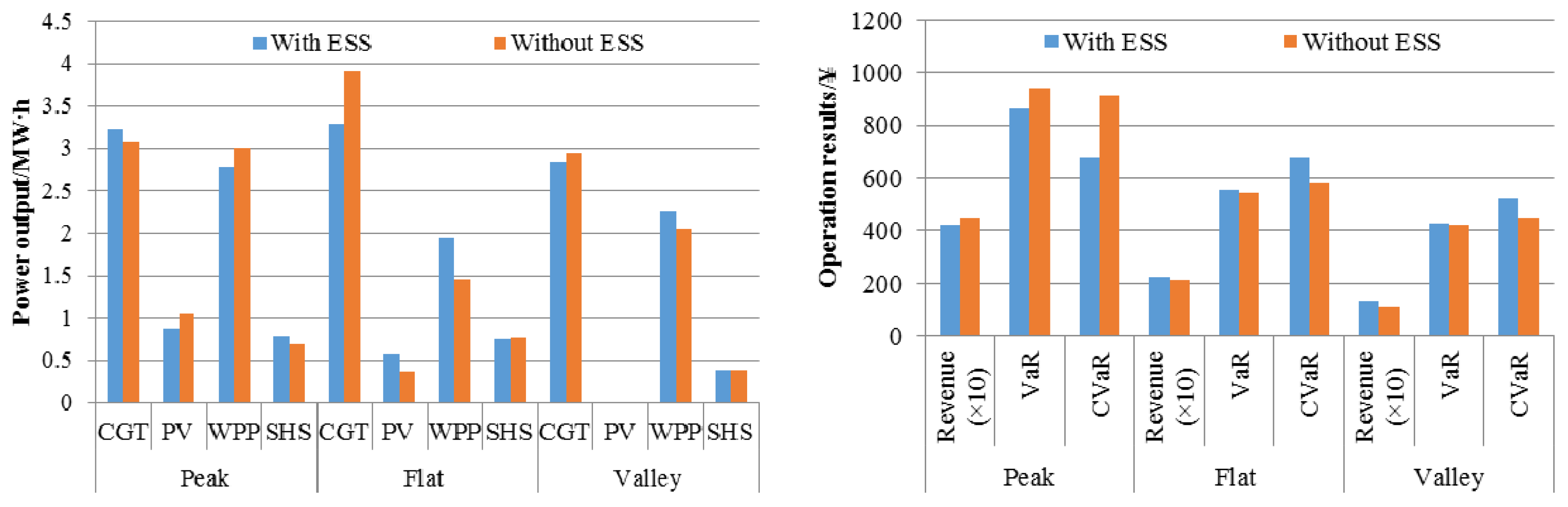
5.3.1. The Impact of ESS on VPP Operation
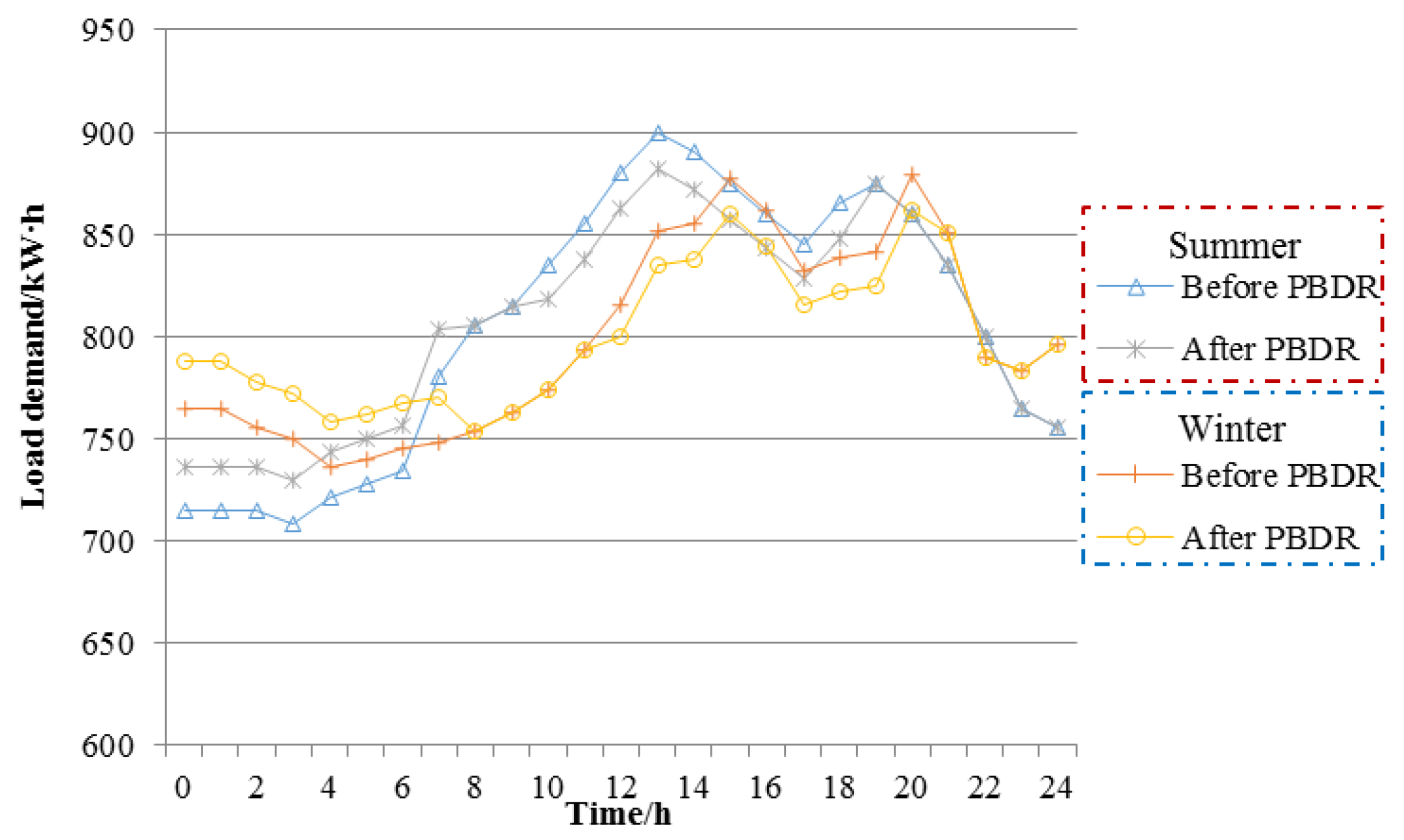
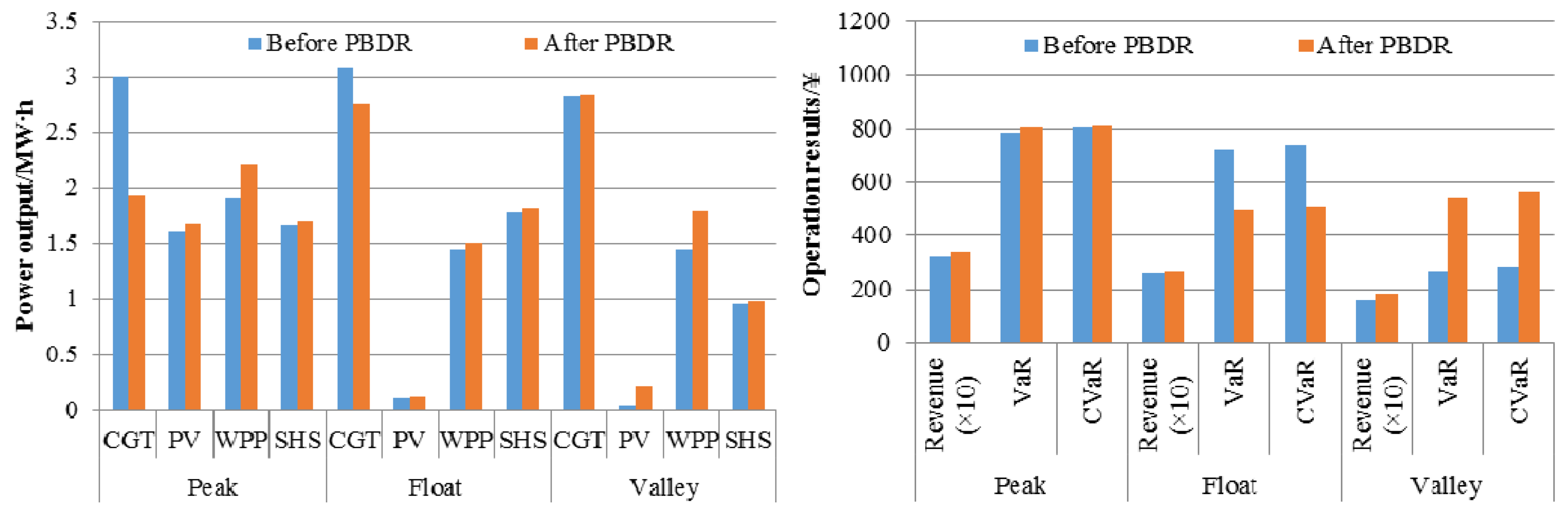
5.3.2. The Impact of PBDR on VPP Operation
5.3.3. The Impact of Linearization on VPP Operation
6. Conclusions
Author Contributions
Funding
Conflicts of Interest
References
- Han, H.T.; Cui, H.T.; Gao, S.; Shi, Q.; Fan, A.; Wu, C. A Remedial Strategic Scheduling Model for Load Serving Entities Considering the Interaction between Grid-Level Energy Storage and Virtual Power Plants. Energies 2018, 11, 2420. [Google Scholar] [CrossRef]
- Riccardo, I.; Benjamin, M.; Tetsuo, T. The Synergies of Shared Autonomous Electric Vehicles with Renewable Energy in a Virtual Power Plant and Microgrid. Energies 2018, 11, 2016. [Google Scholar]
- Zhang, J.C.; Seet, B.C.; Lie, T.T. An Event-Based Resource Management Framework for Distributed Decision-Making in Decentralized Virtual Power Plants. Energies 2016, 9, 595. [Google Scholar] [CrossRef] [Green Version]
- Liu, Z.Y.; Zheng, F.; Wang, L.; Zou, B.; Wen, F.; Xue, Y. Optimal Dispatch of a Virtual Power Plant Considering Demand Response and Carbon Trading. Energies 2018, 11, 1488. [Google Scholar] [CrossRef]
- European Virtual Fuel Cell Power Plant Management Summary Report [EB/OL]. Available online: ftp://ftp.ee.polyu.edu.hk/zhaoxu/power%20system%20literature/euvpp.pdf (accessed on 13 August 2018).
- Xie, J.; Cao, C. Non-Convex Economic Dispatch of a Virtual Power Plant via a Distributed Randomized Gradient-Free Algorithm. Energies 2017, 10, 1051. [Google Scholar] [CrossRef]
- Ju, L.W.; Li, H.H.; Zhao, J.W.; Chen, K.; Tan, Q.; Tan, Z. Multi-objective stochastic scheduling optimization model for connecting a virtual power plant to wind-photovoltaic-electric vehicles considering uncertainties and demand response. Energy Conver. Manag. 2016, 128, 160–177. [Google Scholar] [CrossRef]
- Dong, W.L.; Wang, Q.; Yang, L. A coordinated dispatching model for distribution utility and virtual power plants with wing/photovoltaic/hydro generators. Autom. Electr. Power Syst. 2015, 39, 75–82. [Google Scholar]
- Wang, J.M.; Yang, W.H.; Chen, H.X.; Huang, L.; Gao, Y. The Optimal Configuration Scheme of the Virtual Power Plant Considering Benefits and Risks of Investors. Energies 2017, 10, 968–979. [Google Scholar] [CrossRef]
- Project Interim Report [R/OL]. Available online: http://www.web2energy.com/ (accessed on 20 February 2013).
- Ju, L.W.; Tan, Z.F.; Yuan, J.Y.; Tan, Q.; Li, H.; Dong, F. A bi-level stochastic scheduling optimization model for a virtual power plant connected to a wind–photovoltaic–energy storage system considering the uncertainty and demand response. Appl. Energy 2016, 171, 184–199. [Google Scholar] [CrossRef] [Green Version]
- Pang, Z.H.; Kong, Y.L.; Pang, J.M.; Hu, S.; Wang, J. Geothermal Resources and Development in Xiongan New Area. Bull. Chin. Acad. Sci. 2017, 32, 1224–1230. [Google Scholar]
- Can Kao Xiao Xi. Available online: http://www.cankaoxiaoxi.com/china/20170524/2034700.shtml (accessed on 24 May 2017).
- National Development and Reform Commission. Available online: http://www.ndrc.gov.cn/gzdt/201608/t20160818_815086.html (accessed on 5 August 2016).
- Muhammad, F.Z.; Elhoussin, E.; Mohamed, B. Microgrids energy management systems: A critical review on methods, solutions, and prospects. Appl. Energy 2018, 222, 1033–1055. [Google Scholar]
- Aboelsood, Z.; Hossam, A.G.; Ahmed, E. Optimal planning of combined heat and power systems within microgrids. Energy 2015, 93, 235–244. [Google Scholar]
- Bai, H.; Miao, S.H.; Ran, X.H.; Ye, C. Optimal Dispatch Strategy of a Virtual Power Plant Containing Battery Switch Stations in a Unified Electricity Market. Energies 2015, 8, 2268–2289. [Google Scholar] [CrossRef] [Green Version]
- Cao, C.; Xie, J.; Yue, D.; Huang, C.; Wang, J.; Xu, S.; Chen, X. Distributed Economic Dispatch of Virtual Power Plant under a Non-Ideal Communication Network. Energies 2017, 10, 235. [Google Scholar] [CrossRef]
- Liu, Y.Y.; Li, M.; Lian, H.B.; Tang, X.; Liu, C.; Jiang, C. Optimal dispatch of virtual power plant using interval and deterministic combined optimization. Inter. J. Electr. Power Energy Syst. 2018, 102, 235–244. [Google Scholar] [CrossRef]
- Faeze, B.; Masoud, H.; Shahram, J. Optimal electrical and thermal energy management of a residential energy hub, integrating demand response and energy storage system. Energy Build. 2015, 90, 65–75. [Google Scholar]
- Mashhour, E.; Moghaddas, M.S. Bidding strategy of virtual power plant for participating in energy and spinning reserve markets: Part I problem formulation. IEEE Trans. Power Syst. 2011, 26, 949–956. [Google Scholar] [CrossRef]
- Tascikaraoglu, A.; Erdinc, O.; Uzunoglu, M.; Karakas, A. An adaptive load dispatching and forecasting strategy for a virtual power plant including renewable energy conversion units. Appl. Energy 2014, 119, 445–453. [Google Scholar] [CrossRef]
- Mohammadi, J.; Rahimikian, A.; Ghazizadeh, M.S. Aggregated wind power and flexible load offering strategy. IET Renew. Power Gener. 2007, 5, 439–447. [Google Scholar] [CrossRef]
- Shayeghi, H.; Sobhani, B. Integrated offering strategy for profit enhancement of distributed resources and demand response in microgrids considering system uncertainties. Energy Convers. Manag. 2014, 87, 765–777. [Google Scholar] [CrossRef]
- Shropshire, D.; Purvins, A.; Papaioannou, I.; Maschio, I. Benefits and cost implications from integrating small flexible nuclear reactors with offshore wind farms in a virtual power plant. Energy Policy 2012, 46, 558–573. [Google Scholar] [CrossRef]
- Riveros, J.Z.; Bruninx, K.; Poncelet, K. Bidding strategies for virtual power plants considering CHPs and intermittent renewables. Energy Convers. Manag. 2015, 103, 408–418. [Google Scholar] [CrossRef]
- Hrvoje, P.; Juan, M.; Antonio, J.C.; Kuzle, I. Offering model for a virtual power plant based on stochastic programming. Appl. Energy 2013, 105, 282–292. [Google Scholar]
- Heredia, F.J.; Rider, M.J.; Corchero, C. Optimal bidding strategies for thermal and generic programming units in the dayahead electricity market. IEEE Trans. Power Syst. 2010, 25, 1504–1518. [Google Scholar] [CrossRef] [Green Version]
- Peik-Herfeh, M.; Seifi, H.; Sheikh-El-Eslami, M.K. Decision making of a virtual power plant under uncertainties for bidding in a day-ahead market using point estimate method. Int. J. Electr. Power Energy Syst. 2013, 44, 88–98. [Google Scholar] [CrossRef]
- Yang, H.M.; Yi, D.X.; Zhao, J.H.; Luo, F.; Dong, Z. Distributed optimal dispatch of virtual power plant based on ELM transformation. Management 2014, 10, 1297–1318. [Google Scholar] [CrossRef] [Green Version]
- Zamani, A.G.; Zakariazadeh, A.; Jadid, S. Day-ahead resource scheduling of a renewable energy based virtual power plant. Appl. Energy 2016, 169, 324–340. [Google Scholar] [CrossRef]
- Tan, Z.F.; Wang, G.; Ju, L.W.; Tan, Q.; Yang, W. Application of CVaR risk aversion approach in the dynamical scheduling optimization model for virtual power plant connected with wind-photovoltaic-energy storage system with uncertainties and demand response. Energy 2017, 124, 198–213. [Google Scholar] [CrossRef]
- Morteza, S.; Mohammad-Kazem, S.; Mahmoud-Reza, H. An interactive cooperation model for neighboring virtual power plants. Appl. Energy 2017, 200, 273–289. [Google Scholar]
- Ju, L.W.; Tan, Z.F.; Li, H.H.; Tan, Q.; Yu, X.; Song, X. Multi-objective operation optimization and evaluation model for CCHP and renewable energy based hybrid energy system driven by distributed energy resources in China. Energy 2016, 111, 322–340. [Google Scholar] [CrossRef]
- Yang, Q.; Yuan, Y.; Wang, M.; Zhou, J.; Bao, J.; Zhang, C. Optimal capacity configuration of standalone hydro-photovoltaic-storage microgrid. Electr. Power Autom. Equip. 2015, 35, 37–44. [Google Scholar]


| Time&price | PBDR | IBDR | |||||
|---|---|---|---|---|---|---|---|
| Peak Period | Valley Period | Flat Period | Energy Market | Reserve Market | |||
| Up | Down | ||||||
| Time divide | Summer | 10:00−18:00 | 0:00−7:00 | 8:00−9:00&19:00−24:00 | |||
| Winter | 12:00−20:00 | 0:00−7:00 | 8:00−11:00&21:00−24:00 | ||||
| Power price (¥/kW·h) | 0.69 | 0.33 | 0.55 | 0.5 | 0.2 | 0.6 | |
| Typical Day | Power Output/MW·h | Abandoned Energy/MW·h | Revenue/¥ | |||||||
|---|---|---|---|---|---|---|---|---|---|---|
| CGT | PV | WPP | SHS | ESS | IBDR | WPP | PV | SHS | ||
| Summer | 7.562 | 2.09 | 5.517 | 4.652 | (0.25, −0.24) | (0.36, −0.39) | 0.48 | 0.11 | 0.245 | 7804.85 |
| Winter | 7.282 | 1.673 | 8.566 | 2.058 | (0.20, −0.20) | (0.21, −0.18) | 0.745 | 0.146 | 0.179 | 8265.32 |
| β | Summer | Winter | ||||||||||||
|---|---|---|---|---|---|---|---|---|---|---|---|---|---|---|
| Power Output/MW·h | CVaR/¥ | Power Output/MW·h | CVaR/¥ | |||||||||||
| CGT | PV | WPP | SHS | ESS | IBDR | CGT | PV | WPP | SHS | ESS | IBDR | |||
| 0.8 | 8.06 | 1.95 | 5.43 | 4.50 | (0.3, −0.3) | (0.36, −0.30) | 1764.58 | 7.61 | 1.61 | 8.43 | 2.01 | (0.35, −0.33) | (0.33, −0.27) | 1878.18 |
| 0.85 | 8.18 | 1.92 | 5.32 | 4.47 | (0.35, −0.36) | (0.36, −0.24) | 1740.27 | 7.80 | 1.59 | 8.26 | 2.00 | (0.4, −0.36) | (0.30, −0.24) | 1852.30 |
| 0.90 | 8.49 | 1.87 | 5.10 | 4.41 | (0.4, −0.4) | (0.33, −0.18) | 1725.59 | 8.19 | 1.55 | 7.91 | 1.97 | (0.45, −0.44) | (0.27, −0.18) | 1836.67 |
| 0.95 | 8.53 | 1.83 | 5.02 | 4.39 | (0.5, −0.4) | (0.33, −0.15) | 1713.89 | 8.31 | 1.51 | 7.79 | 1.96 | (0.50, −0.48) | (0.27, −0.15) | 1824.22 |
| 0.98 | 8.83 | 1.75 | 4.85 | 4.36 | (0.5, −0.44) | (0.30, −0.15) | 1703.36 | 8.67 | 1.45 | 7.53 | 1.95 | (0.5, −0.48) | (0.24, −0.15) | 1813.01 |
| Typical Day | Power Output/MW·h | Operation Results/¥ | ||||||||
|---|---|---|---|---|---|---|---|---|---|---|
| CGT | PV | WPP | SHS | ESS | IBDR | Revenue | VaR | CVaR | ||
| Summer | Case 1 | 7.562 | 2.09 | 5.517 | 4.652 | (0.25, −0.24) | (0.36, −0.39) | 7804.85 | ||
| Case 2 | 8.49 | 1.870 | 5.104 | 4.41 | (0.40, −0.40) | (0.33, −0.18) | 7645.50 | 1716.77 | 1725.59 | |
| Case 3 | 8.921 | 1.760 | 4.797 | 4.407 | (0.30, −0.28) | (0.09, −0.15) | 7440.70 | 1785.48 | 1824.35 | |
| Winter | Case 1 | 7.282 | 1.673 | 8.566 | 2.058 | (0.20, −0.20) | (0.21, −0.18) | 8265.32 | − | − |
| Case 2 | 8.190 | 1.550 | 7.912 | 1.97 | (0.45, −0.44) | (0.27, −0.18) | 8137.68 | 1827.29 | 1836.67 | |
| Case 3 | 9.342 | 1.455 | 6.984 | 1.901 | (0.30, −0.24) | (0.09, −0.09) | 7793.98 | 1842.36 | 1875.48 | |
| Capacity/ MW·h | Power Output/MW·h | Operation Results/¥ | |||||||
|---|---|---|---|---|---|---|---|---|---|
| CGT | PV | WPP | SHS | ESS | IBDR | Revenue | VaR | CVaR | |
| 0 | 9.941 | 1.419 | 6.517 | 1.834 | 0 | (0.15, −0.15) | 7645.54 | 1905.430 | 1938.840 |
| 0.2 | 9.342 | 1.455 | 6.984 | 1.901 | (0.3, −0.24) | (0.09, −0.09) | 7793.98 | 1842.362 | 1875.48 |
| 0.4 | 8.983 | 1.497 | 7.176 | 1.935 | (0.36, −0.3) | (0.12, −0.12) | 7867.843 | 1833.789 | 1869.525 |
| 0.6 | 8.682 | 1.539 | 7.316 | 1.965 | (0.45, −0.39) | (0.12, −0.15) | 7937.503 | 1822.579 | 1860.852 |
| 0.8 | 8.351 | 1.581 | 7.504 | 1.975 | (0.51, −0.45) | (0.15, −0.18) | 8028.115 | 1810.506 | 1851.539 |
| 1.0 | 8.199 | 1.602 | 7.599 | 1.982 | (0.54, −0.48) | (0.15, −0.18) | 8065.874 | 1795.140 | 1836.481 |
| Peak-to-Valley Price Gap | Load Demand/MW | Peak-to-Valley Ratio | Clean Energy Output/MW·h | Revenue/ ¥ | VaR /¥ | CVaR /¥ | |||
|---|---|---|---|---|---|---|---|---|---|
| Max | Min | PV | WPP | SHS | |||||
| 1 | 0.900 | 0.709 | 1.270 | 1.76 | 4.797 | 4.407 | 7440.7 | 1785.48 | 1824. 35 |
| 2 | 0.891 | 0.723 | 1.233 | 1.848 | 5.037 | 4.440 | 7584.963 | 1805.447 | 1844.457 |
| 2.6 | 0.882 | 0.730 | 1.209 | 2.024 | 5.517 | 4.505 | 7873.49 | 1845.38 | 1884.67 |
| 3 | 0.878 | 0.733 | 1.197 | 2.141 | 5.837 | 4.549 | 8065.841 | 1872.002 | 1911.479 |
| 3.5 | 0.876 | 0.735 | 1.192 | 2.200 | 5.997 | 4.570 | 8162.017 | 1885.313 | 1924.883 |
| cases | MIP | MINLP | Time/s | |||||
|---|---|---|---|---|---|---|---|---|
| Revenue/¥ | VaR/¥ | CVaR/¥ | Revenue/¥ | VaR/¥ | CVaR/¥ | MINLP | MIP | |
| Case 1 | 7804.85 | 7895.96 | 245 s | 10 s | ||||
| Case 2 | 7645.50 | 1716.77 | 1725.59 | 7442.65 | 1785.27 | 1893.48 | 278 s | 14 s |
| Case 3 | 7440.70 | 1785.48 | 1824.35 | 7305.45 | 1805.45 | 1905.12 | 304 s | 18 s |
© 2018 by the authors. Licensee MDPI, Basel, Switzerland. This article is an open access article distributed under the terms and conditions of the Creative Commons Attribution (CC BY) license (http://creativecommons.org/licenses/by/4.0/).
Share and Cite
Ju, L.; Li, P.; Tan, Q.; Tan, Z.; De, G. A CVaR-Robust Risk Aversion Scheduling Model for Virtual Power Plants Connected with Wind-Photovoltaic-Hydropower-Energy Storage Systems, Conventional Gas Turbines and Incentive-Based Demand Responses. Energies 2018, 11, 2903. https://doi.org/10.3390/en11112903
Ju L, Li P, Tan Q, Tan Z, De G. A CVaR-Robust Risk Aversion Scheduling Model for Virtual Power Plants Connected with Wind-Photovoltaic-Hydropower-Energy Storage Systems, Conventional Gas Turbines and Incentive-Based Demand Responses. Energies. 2018; 11(11):2903. https://doi.org/10.3390/en11112903
Chicago/Turabian StyleJu, Liwei, Peng Li, Qinliang Tan, Zhongfu Tan, and GejiriFu De. 2018. "A CVaR-Robust Risk Aversion Scheduling Model for Virtual Power Plants Connected with Wind-Photovoltaic-Hydropower-Energy Storage Systems, Conventional Gas Turbines and Incentive-Based Demand Responses" Energies 11, no. 11: 2903. https://doi.org/10.3390/en11112903