Simulation and Comparison of Mathematical Models of PV Cells with Growing Levels of Complexity


1
Management and Production Technologies of Northern Aveiro—ESAN, Estrada do Cercal, 449, Santiago de Riba-Ul, 3720-509 Oliveira de Azeméis, Portugal
2
C-MAST—Centre for Aerospace Science and Technologies—Department of Electromechanical Engineering, University of Beira Interior, 6201-001 Covilhã, Portugal
3
Faculty of Engineering and Environment, Department of Physics and Electrical Engineering, Northumbria University Newcastle, Newcastle upon Tyne NE18ST, UK
4
Department of Electrical Engineering and Automation, Aalto University, 02150 Espoo, Finland
*
Author to whom correspondence should be addressed.
Energies 2018, 11(11), 2902; https://doi.org/10.3390/en11112902
Submission received: 24 September 2018
/
Revised: 15 October 2018
/
Accepted: 23 October 2018
/
Published: 25 October 2018
(This article belongs to the Special Issue Solar Energy Harvesting, Storage and Utilization)
Abstract
:The amount of energy generated from a photovoltaic installation depends mainly on two factors—the temperature and solar irradiance. Numerous maximum power point tracking (MPPT) techniques have been developed for photovoltaic systems. The challenge is what method to employ in order to obtain optimum operating points (voltage and current) automatically at the maximum photovoltaic output power in most conditions. This paper is focused on the structural analysis of mathematical models of PV cells with growing levels of complexity. The main objective is to simulate and compare the characteristic current-voltage (I-V) and power-voltage (P-V) curves of equivalent circuits of the ideal PV cell model and, with one and with two diodes, that is, equivalent circuits with five and seven parameters. The contribution of each parameter is analyzed in the particular context of a given model and then generalized through comparison to a more complex model. In this study the numerical simulation of the models is used intensively and extensively. The approach utilized to model the equivalent circuits permits an adequate simulation of the photovoltaic array systems by considering the compromise between the complexity and accuracy. By utilizing the Newton–Raphson method the studied models are then employed through the use of Matlab/Simulink. Finally, this study concludes with an analysis and comparison of the evolution of maximum power observed in the models.
1. Introduction
The Energy Union Framework Strategy is aiming to a serious transition from an economy dependent on fossil fuels to one more reliant on renewables [1] and among the available sources of renewable energy, solar energy is on the most abundant [2,3,4], which could be assertively harnessed, especially in the southern countries of Europe. According to Club of Rome study embracing the circular economy concept could signify up to 70% decrease in carbon emissions by 2030, of five European economies [5]. By targeting a renewable energy based economy and a circular economy at the same time could be the way achieve the Energy Union Framework Strategy targets [1]. Although free and available on a planetary scale, the role in the global energy mix is unobtrusive, competing not only with other forms of non-renewable energy, such as gas and coal [6], but also with its more direct rival—the wind renewable energy source [7]. Except for a very limited number of countries where proactive and generous income policies were implemented at the beginning of the last decade, there has been a more recent mobilization of European governments in this sector, legislating on specific instruments to stimulate production decentralized and small scale power [8]. In the last few years, the solar energy has been gaining importance in the worldwide energy evolution tendency due to a constantly increasing efficiency and lifespan, the decrease of the price of PV modules and by being environmentally friendly [9]. Solar photovoltaic (PV) systems are steadily becoming one of the main three electricity sources in Europe [10]. The entire installed PV capacity in 2016 reached 303 GWp and in that year Spain and Italy were responsible for 5.4 and 19.3 GWp, respectively [11].
In a typical PV system several photovoltaic modules are linked in series in order to create a PV string. The aim is to reach a certain voltage and power output. With the intention of accomplishing a greater power, such PV strings can be linked in parallel in order to make a PV array. For the duration of a constant irradiance condition, the power-voltage (P-V curve) characteristics of a PV string show a typical P-V curve peak. Such type of a peak embodies the maximum power of the PV string [4]. The P-V characteristics of a PV system are nonlinear and are affected by both the ambient temperature and solar irradiance, which in turn reveal distinct MPPs. With the purpose of optimizing the use of PV systems, conventional MPPT algorithms are often used [12].
In the planning of a photovoltaic power plant the electric power produced is strongly linked to the meteorological conditions (solar radiation and temperature) [13,14]. Due to the intermittent nature of solar energy, power forecasting is crucial for a correct interpretation of business profitability and payback time [15]. In the current market there is a great offer of manufacturers that, of course, have quite different technological production processes. All this leads to two modules with an identical technical sheet, under nominal test conditions, to differ in performance and produce very different results [16]. The actual operating conditions in both solar radiation and temperature will very rarely coincide with the combination of nominal meteorological variables. Thus, the broader characterization is of utmost importance for studying the differences [17]. In the end the main goal is to realistically quantify the performance, giving credibility to the estimation process in function of meteorological specificities of each season of the year. Ultimately it is desired that the process has enough resolution to reach the count up to the daily cycle.
The characterization requires the compilation of a large amount of data required for the application of appropriate mathematical model. In the concrete case of the photovoltaic cell the analytical model opens the doors for the detailed description in function of the external variables, which for all effects determine the general forms of the characteristic curves. However, to make modeling effective, it will be the model’s intrinsic parameters which will more or less shape the link to the experimental data [18]. Molding is particularly critical at three points of operation. First, the predicted forecast of the peak electric power, then the open circuit operating points, that is, the maximum potential difference to be supported by the power electronics in the DC-AC conversation in the cut-off state, and finally the short-circuit, that is the maximum current to be supported by the electric cables in the event of a fault.
The models share in common the same electrical base model. The cell being a photoelectric device is modeled with a DC current source and a junction diode in parallel. From here all models are effectively variations with the introduction of more electrical elements. The elements may be of a series element of resistive nature by recreating the internal losses by Joule, or a parallel resistance simulating the internal leakage current, or a supplementary diode, which is normally associated with the losses by recombination of the carriers in the zone of the depletion layer [19].
Researchers have been increasingly focusing on MPPT techniques [20,21,22,23,24]. Authors in [25] have proposed a glowworm swarm optimization-based MPPT for PVs exposed to uneven temperature distribution and solar irradiation. A technique based on Radial Movement Optimization (RMO) for detecting the MPPT under partial shading conditions and then compared with the results of the particle swarm optimization (PSO) method is studied in [19]. Authors in [26] focus on the analysis of dynamic characteristic for solar arrays in series and MPPT based on optimal initial value incremental conductance strategy under partially shaded conditions. In [27] the authors optimize the MPPT with a model of a photovoltaic panel with two diodes in which the solution is implemented by Pattern Search Techniques. A PV source that was made by utilizing un-illuminated solar panels and a DC power supply that functions in current source mode is proposed in [18]. The authors in [28] address a simple genetic algorithm (GA)—based MPPT method and then compare the experimental and theoretical results with conventional methods. A direct and fully explicit method of extracting the solar cell parameters from the manufacturer datasheet is tested and presented in [29] and the authors base their method on analytical formulation which includes the use of the Lambert W-function with the aim of turning the series resistor equation explicit. The authors in propose a three-point weight method shared with fuzzy logic for increasing the speed of MPPT [30] and in this study the simulation was performed in Matlab and was experimentally validated.
The followed methodology was made for the comparison of the models in meteorological conditions as wide as possible. Extreme scenarios of incident solar radiation were simulated. The simulated temperature was considered suitable. The main goal of this study is to simulate and compare the characteristic curves of equivalent circuits of the ideal PV cell and, with one and with two diodes, respectively, namely equivalent circuits with five and seven parameters. The role of every parameter is assessed and compared. The ideal model of the PV cell is given in detail in [31]. The aim was to find areas of model intervention in which the modeling could lead to identical results. In this study the numerical simulation of the models is used intensively and extensively. The method used to model the equivalent circuits allows an adequate simulation of the photovoltaic array systems by taking into consideration the compromise between accuracy and complexity. By using the Newton–Raphson method the studied models are simulated through the use of Matlab/Simulink. All the simulations were carried out on the basis of a solar cell whose electrical specifications are given in [32].
The remainder of this paper is organized as follows. In Section 2 the equivalent circuit with five parameters is presented while in Section 3 the equivalent circuit with seven parameters is presented. The comparison between the one-diode model and the two-diode model is presented in Section 4. Finally, the conclusions are addressed in Section 5.
2. Equivalent Circuit with Five Parameters
2.1. Representative Equations
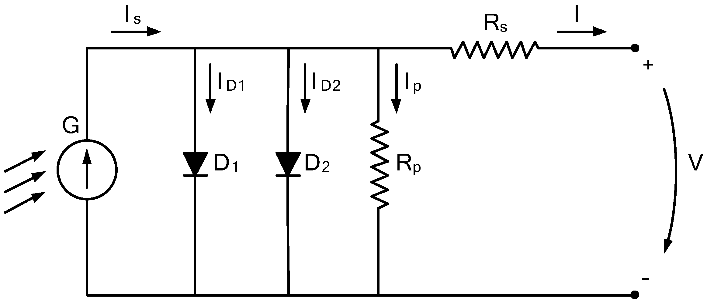
The five-parameter circuit completes the frame of internal resistive losses. The fifth parameter corresponds to one more parasite resistance, referred to in this paper as the parallel resistance Rp. Unlike the series resistance (Rs) it does not interfere directly with the power delivered to the load. However, it penalizes the operation of the cell by providing an alternative path for a portion of the photoelectric current. It is called a leakage current because it reduces the amount of current flowing at the PN junction [33], thereby affecting the voltage to the terminals of the photovoltaic cell. The five-parameter electrical circuit is the most widely used model in the analytical study of the photovoltaic cell. This model offers a good compromise in terms of complexity and performance [34], thus being the choice of several authors in this area of research [25,26,28,35,36,37,38]. The model of the equivalent circuit with five parameters of the photovoltaic (PV) module can be observed in Figure 1.
According to the junction or nodal rule the sum of currents is governed by the following condition:
and the voltage in the diode is equivalent to:
Solving in order of I and replacing ID with the diode expression and Ip with Vd/Rp the following equation is obtained:
where Is is the current created by photoelectric effect, Iis is the reverse saturation current, q is the charge of the electron, K is the Boltzmann constant (1.38 × 10⁻²³ J/°K), T is the temperature of the junction, m is the reality parameter, Rs is the parasite resistance in series and Rp is the parallel parasite resistance. The value of Rp is usually quite high in the manufactured photovoltaic cells. However, several authors with regard to this finding, consider useless the inclusion of this resistance [39,40,41,42,43,44]. On the other hand there are authors who consider Rs negligible when the value is very low [45,46,47].
After obtaining the characteristic equation I-V the electrical power is calculated by:
Deriving at the peak of power, one can find the voltage coordinate, as follows:
The solution in order of V is only resolvable if applying an iterative numerical method.
2.2. Analytical Extraction of Parameters
Five equations are required. By consulting the manufacturer’s information under nominal reference conditions the following equations are obtained:
In practice the system is reduced to four algebraic equations. By observing Equation (3) it can be stated that:
This means that it is possible to eliminate the term −1 without degrading the approximation given by the model to the I-V curve. This measure simplifies the analytical resolution of the four variables [48]. Thus, the system is limited to:
The fourth equation is the expression of the power derivative in order of the voltage.
The derivative can be decomposed as a function of V and I:
which leads to:
Since the Equation (3) is the type of I = f(I,V), the implied derivative as a function of I and V is:
and dividing by dV it results in:
By replacing Equation (18) in Equation (15) it is obtained:
Solving the partial derivatives it is reached the explicit expression of the Equation (15):
where the final presentation is:
The system equations do not allow the separation of individual parameters Iis, Rs, Rp, and m through the analytical solution. For this reason, appropriate numerical methods must be used.
2.3. Simulation
2.3.1. Assessing Equations
The inverse saturation current is obtained by Equation (3) and it is referred to the open circuit operating point:
In previous models only the equation of V in order to I required the Newton-Raphson method. If we try to derive the expression of Vca with Equation (3) set under open circuit conditions:
The final result becomes:
The assignment of one more parameter to the circuit structure renders impracticable the analytical resolution of the Equation (3). This means that it is not possible to separate and isolate the variables I and V in each member through elementary functions. Being the expression of the type I = f(I,V) the equation is commonly referred to as transcendental equation. In general, a transcendent equation does not have an exact solution [49]. The only way to find an approximate solution lies in the use of numerical calculation. In this context the Newton-Raphson algorithm was chosen. The Newton-Raphson method is a fairly fast (quadratic) convergence computational technique for calculating the roots of a function [50,51,52]. Due to its simplicity it lends itself perfectly to such problems. Then the Newton-Raphson method is used through its generic expression as shown in Equation (25):
Being xn+1 the estimated value in the present iteration, xn the value obtained in the previous iteration, f(x) the function initialized with xn and the f’(x) the derivative initialized with xn.
Accordingly, Equation (24) takes the form of a transcendental equation. Thus, by using the Newton-Raphson method through its generic expression (25) the voltage Vca can be assessed by:
where Ica becomes a null value.
And the corresponding procedure for current I is:
Knowing that the value of V is an input variable in the algorithm, then for each V there will be the corresponding I, computed iteratively by Equation (27). The convergence process ends when the following error criterion ε is satisfied:
The nominal characteristic curves are obtained with Equations (4), (22), and (27). The remaining scenarios are supported by Equations (4), (26), (27), (29), and (30), where Equation (29) is a cubic relation between the inverse current and the temperature as proposed in [53,54]:
where is the inverse saturation current and Tn is the temperature, both under Standard Test Conditions (STC) reference conditions. Additionally, in this study, the following simplification was taken into account, where G is the incident radiation in W/m2:
2.3.2. Comparison between Constant Rs and Variable Rp
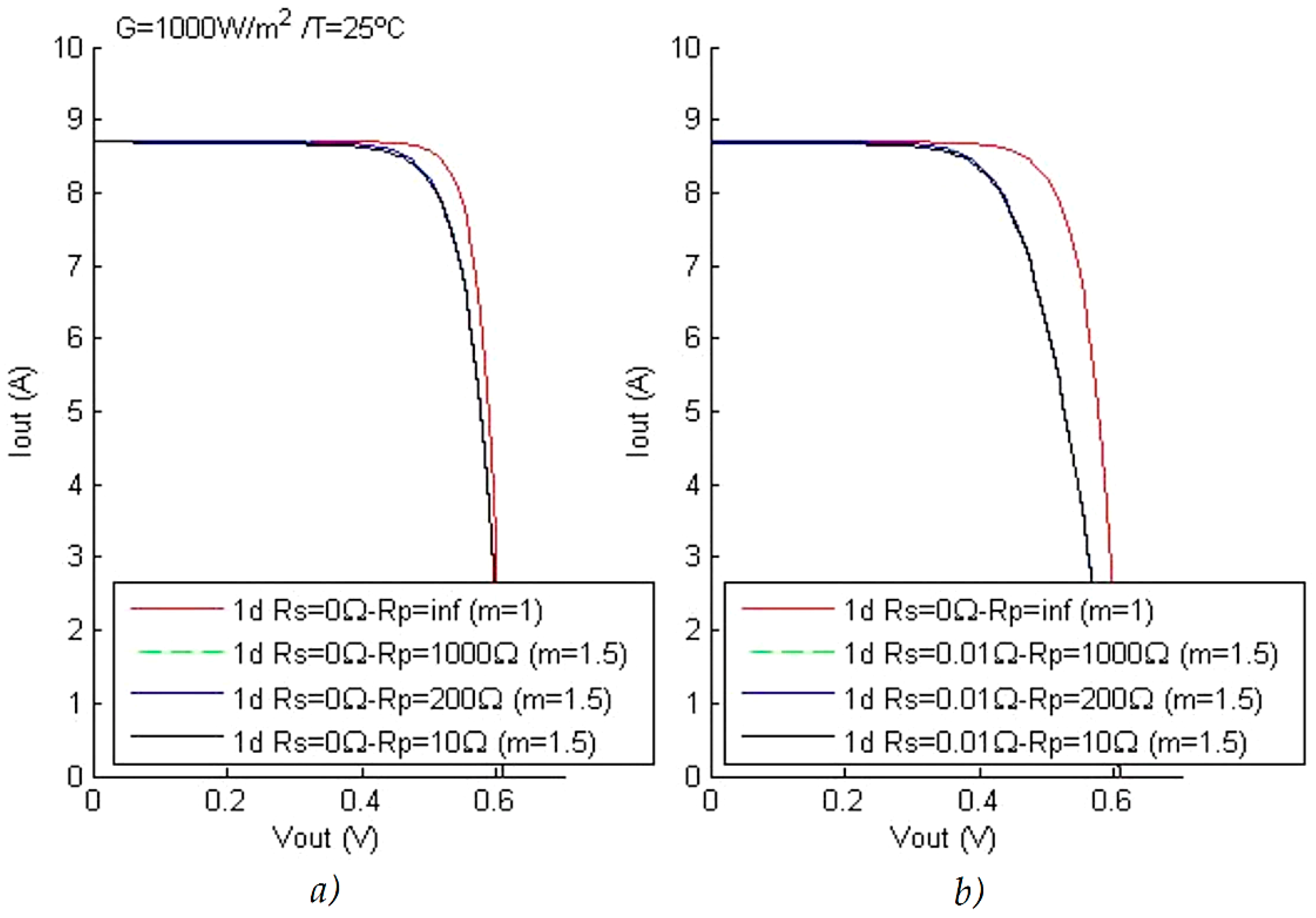
Two comparative scenarios were designed for the characteristic curves at nominal reference conditions. In the first one the load is interconnected to a photovoltaic circuit dominated by resistive losses Rp (Rs = 0). The Rp resistance was adjusted with 10 Ω, 200 Ω, and 1000 Ω, respectively. In the second scenario a fixed value of 10 mΩ was established for the Rs resistor. The simulations can be observed in Figure 2.
By observing the two graphs it is apparent that the resistance Rp does not interfere in the region of influence of the junction diode. In the region where the influence of the photoelectric current source predominates, the lowest value tested does not show a significant disturbance: the plot is very similar to the set of points estimated with Rp = ∞.
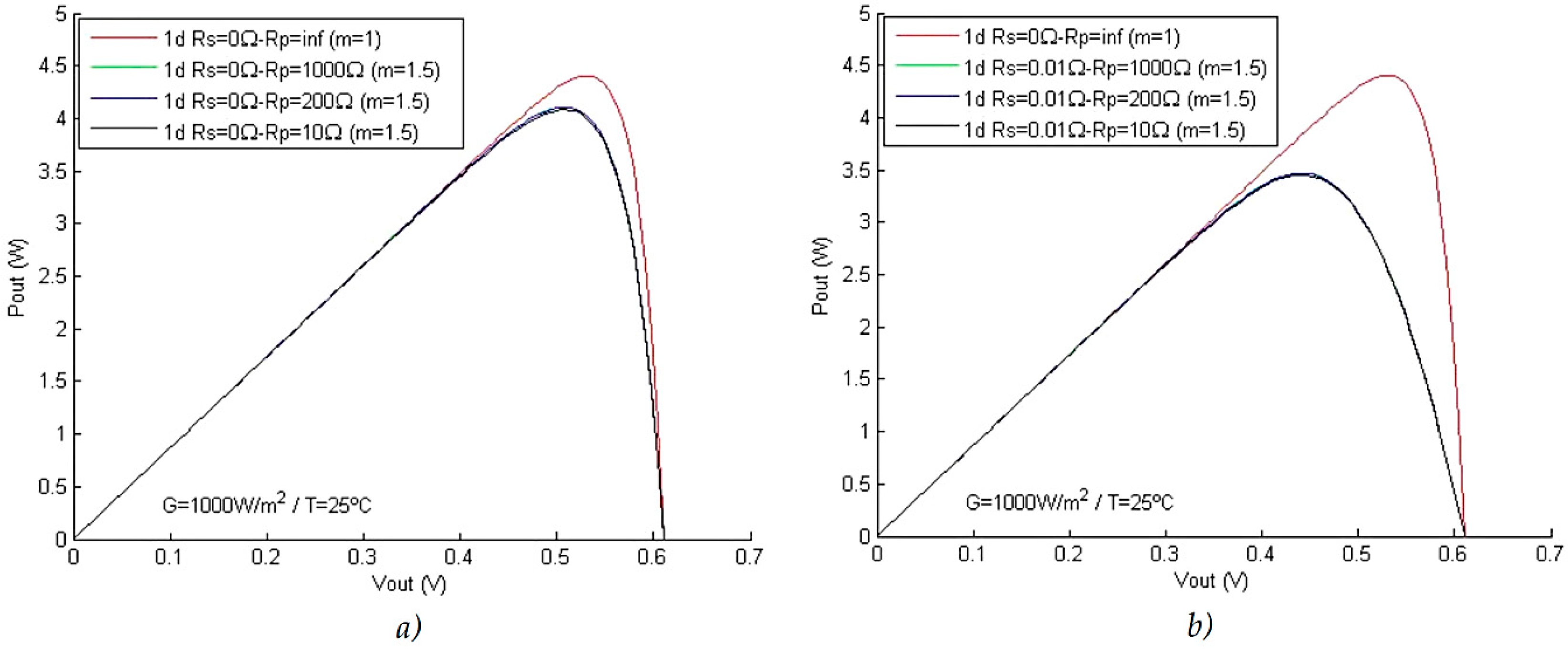
As the figures do not have sufficient detail, the curves were enlarged by a range of values close to the peak power. Figure 3 shows that the leakage current is virtually zero from 200 Ω. While for 10 Ω, the effect being visible is not at all significant. By observing the P-V curves in circuits with internal losses it can be verified that the lines are very similar, as can be in Figure 4. In other words, the leakage of current modelled by the resistance Rp in this range of values does not compromise the estimated maximum power. In this context of temperature and solar radiation this conclusion becomes valid.
2.3.3. Characteristic Curves in Function of Temperature and Radiation
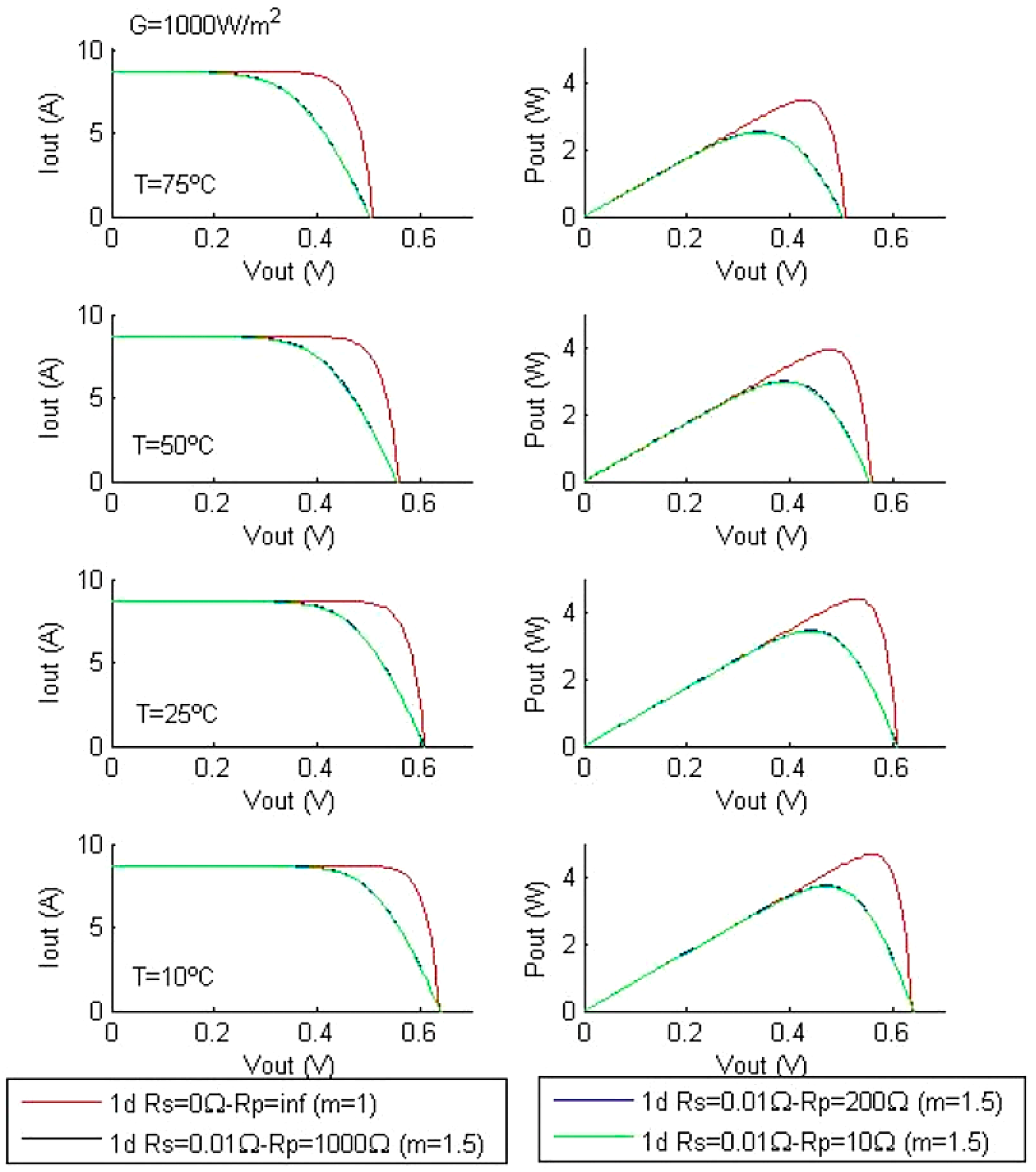
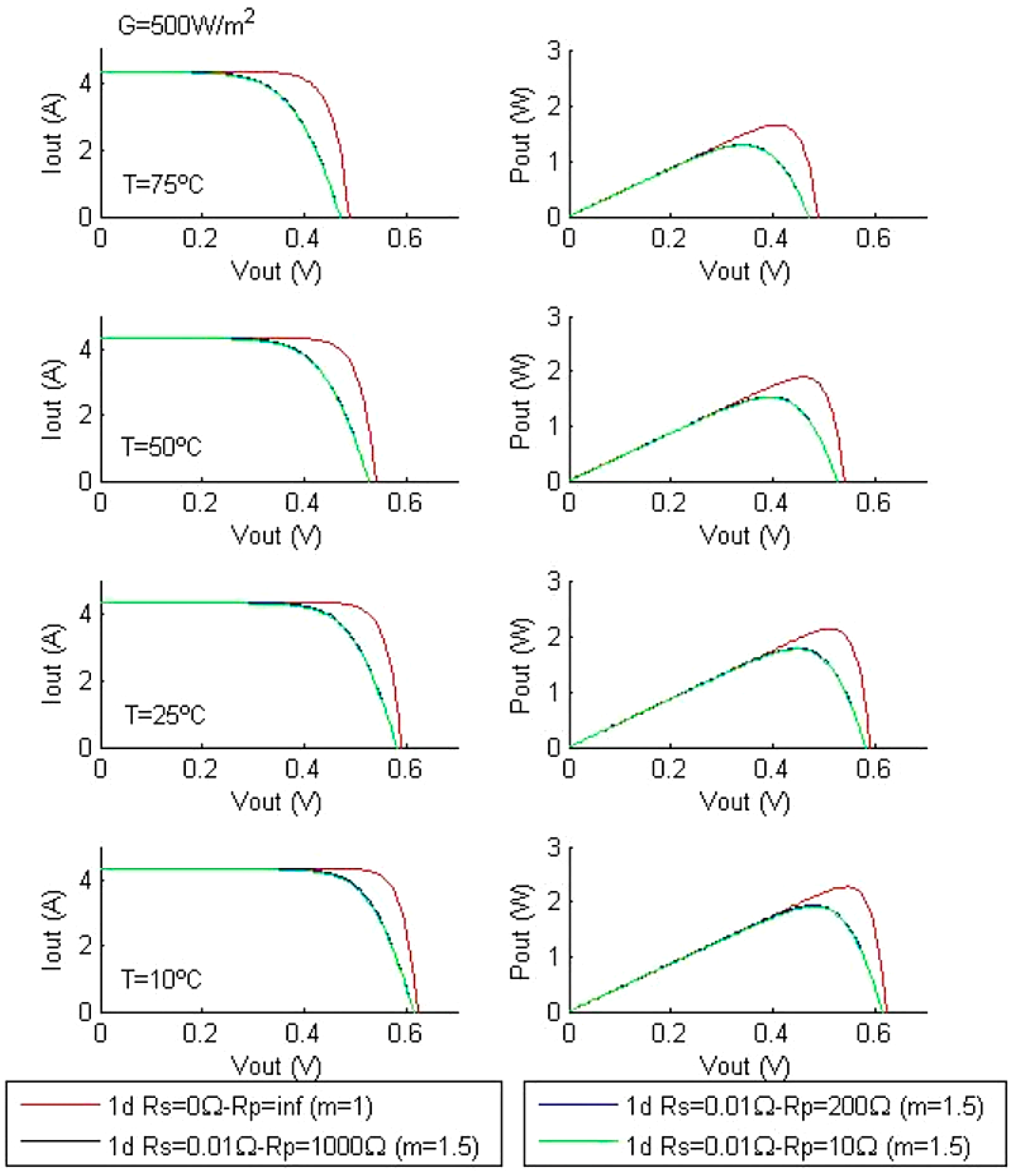
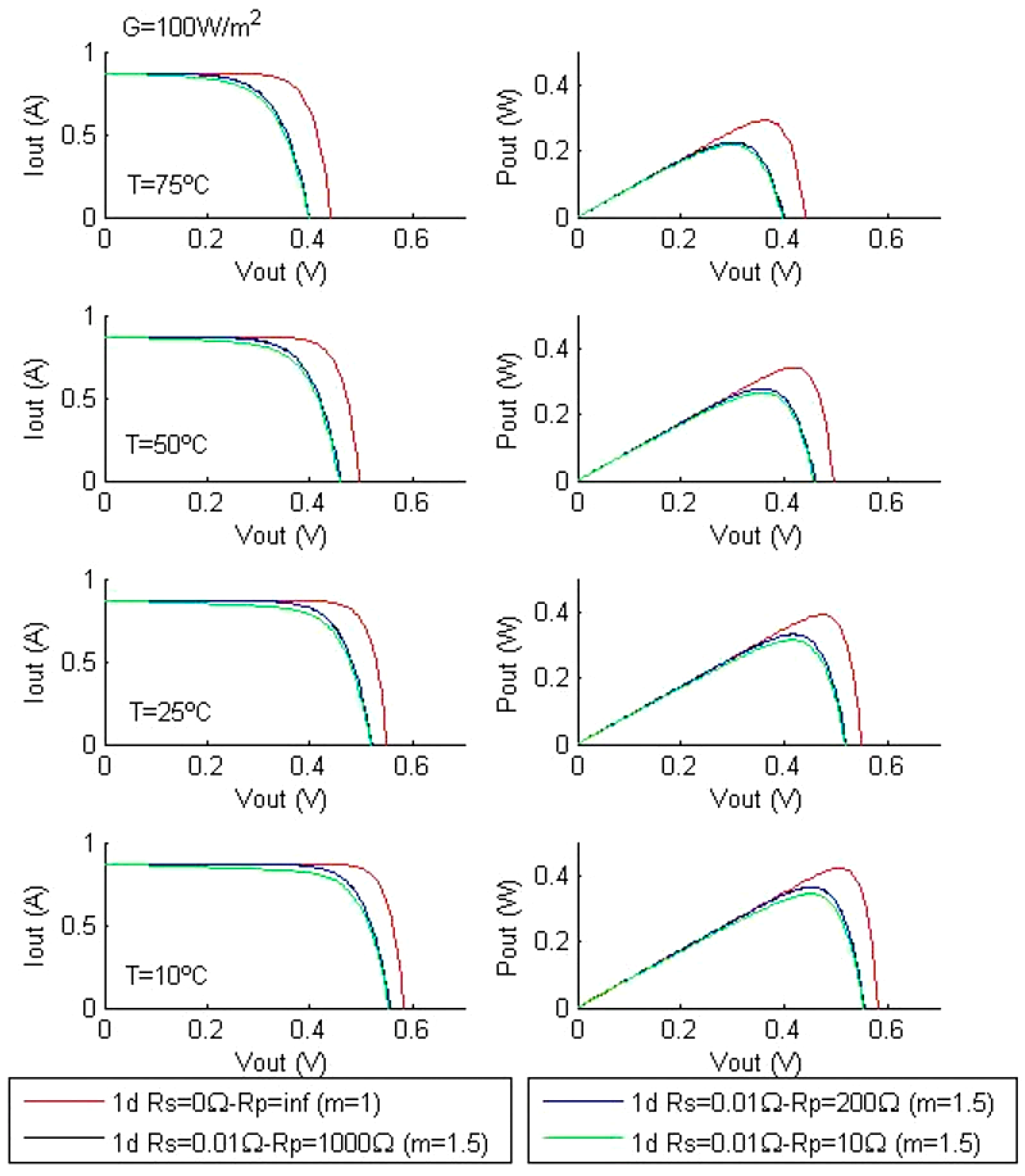
Using the same set of Rp resistors, three data set scenarios are established, as can be observed in Figure 5, Figure 6 and Figure 7. Each scenario is simulated with a specific solar power, 100 W/m2, 500 W/m2, and 1000 W/m2, respectively, and having in common the same interval of test temperatures (10 °C, 25 °C, 50 °C, and 75 °C).
At the higher power range (1000 W/m2) the I-V curves are literally identical. Consequently, the P-V curves do not experience significant changes between 10 °C and 75 °C. The peak power is then identical, regardless of whether the cell is manufactured with a high parallel resistance (1000 Ω) or with considerably low resistance (10 Ω).
At a medium power range (500 W/m2) the performance is matched to that observed in the power ceiling of 1000 W/m2. With the solar radiation reduced to a tenth (100 W/m2) of the highest power range, finally, there is some deviation in the I-V curve, characterized by Rp = 10 Ω. In thermal terms, there is no correlation with Rp: the difference with the versions with higher Rp losses is apparently constant for the analyzed temperature scale.
Summarizing the Figure 4, Figure 5 and Figure 6, it can be concluded that the impact of the parallel resistance on the performance of the cell, is barely expressive in the generality of the tested meteorological conditions, except for a slight disruption of the peak of power with 10 Ω in Rp and under weak incident solar radiation.
3. Equivalent Circuit with Seven Parameters
3.1. Representative Equations
The seven-parameter electrical circuit is the next step in the electrical modeling of the photovoltaic cell. Equivalently to the mono-diode model (five parameters), the full version of two diodes brings together the complete set of losses. The seventh parameter is the leakage current modeled by the parallel resistance Rp. The seven-parameter equivalent electrical circuit with two diodes can be observed in Figure 8.
The sum of currents at the top node is:
The voltage across the two diodes is equivalent to:
Making the appropriate substitutions the final expression of I as a function of V is:
where Is is the photoelectric equivalent current, Iis1 and Iis2 are the saturation currents of diode 1 and diode 2 respectively, m1 and m2 the ideality parameters of diode 1 and diode 2, respectively. As in the previous model, q represents the charge of the electron, K is the Boltzmann constant (1.38 × 10⁻²³ J/°K), T is the temperature of the junction, m is the reality parameter, Rs is the parasite resistance in series and Rp is the parallel parasite resistance.
Despite being computationally more demanding, several authors argue that the approximation is more accurate than that achieved one with less complex models [45,55,56,57,58]. For instance, for a low radiation level, the two-diode model estimates with better approximation than the one-diode model [55,59].
Several authors simplify the identification of the parameters, reducing the number of effectively calculated variables. The most common is the reduction of seven to five variables by specifying fixed values. Usually this practice is related to the parameters m1 and m2 [55,60,61,62]. Other authors opt for complete identification through elaborated methodologies such as particle examination optimization [63], the estimation based on neural networks [64], on genetic algorithms [65] or through algebraic relations as a function of temperature [62].
If the expression of I-V is identified the output electrical power P obeys to:
From where by the derivative of the power peak it is possible to reach the value of V:
Since the expression is transcendental the solution can only be found with a numerical algorithm that is able to extract the root.
3.2. Analytical Extraction of Parameters
Only six equations are required (the variable Is is excluded from the system since the linear dependence with temperature is known) the system is:
As the role of parasite resistance Rs is more pronounced in the vicinity of Vca, an orderly relation to this variable is determined through the derivative of the characteristic expression of the seven-parameter model:
By rearranging this equation around R it becomes as follows:
By replacing V with Vca and I with 0, the Rs is as assessed as follows:
where is an initial estimation of the series resistance for the purposes of iterative numerical calculation.
By using Equation (40) de derived equation of Rp is as follows:
Meaning that in order of Rp it becomes as follows:
The Rp in the vicinity of the short-circuit operating point is represented as follows:
where is an approximate value of the parallel resistance for the purposes of iterative numerical calculation. It is usually estimated with the slope around the short-circuit operating point.
The still missing equation is the derivative of the power P as a function of V at the maximum electric power point. The developed equation takes the form of:
3.3. Assessing the Simulation Equations
The inverse saturation current is determined by Equation (33) at the open circuit operating point with the following analytical expression:
The open circuit voltage Vca is given by:
where Ica is the open circuit current. The current I is given by the following equation:
The current and power strokes in nominal regime are estimated with Equations (34), (47), and (49). In a more comprehensive meteorological frame the calculation is carried out with the Equations (29), (30), (34), (48), and (49).
4. Comparison between the One-Diode Model and the Two-Diode Model
4.1. Characteristic Curves in Function of the Solar Radiation and the Parallel Resistance Rp
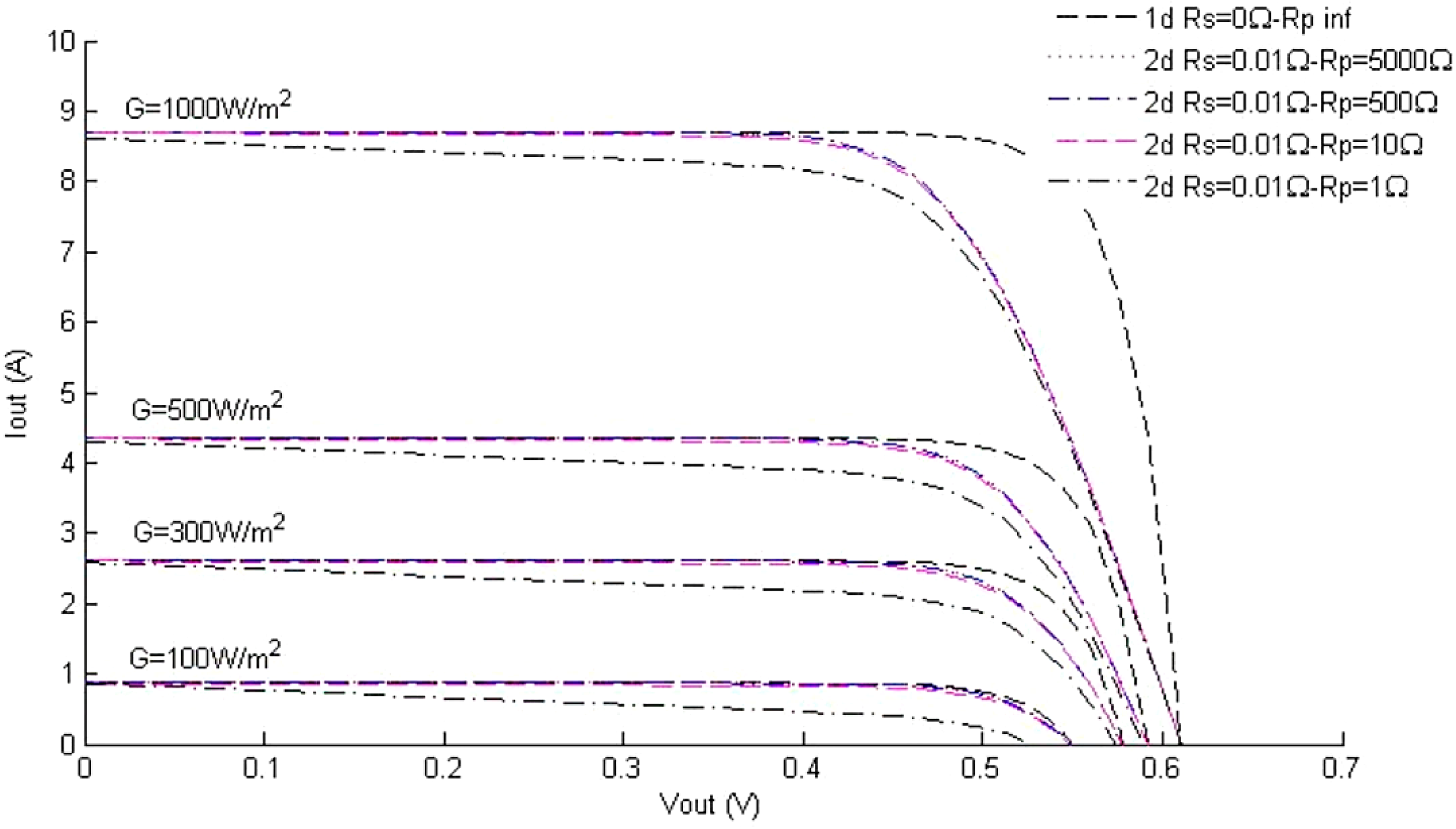
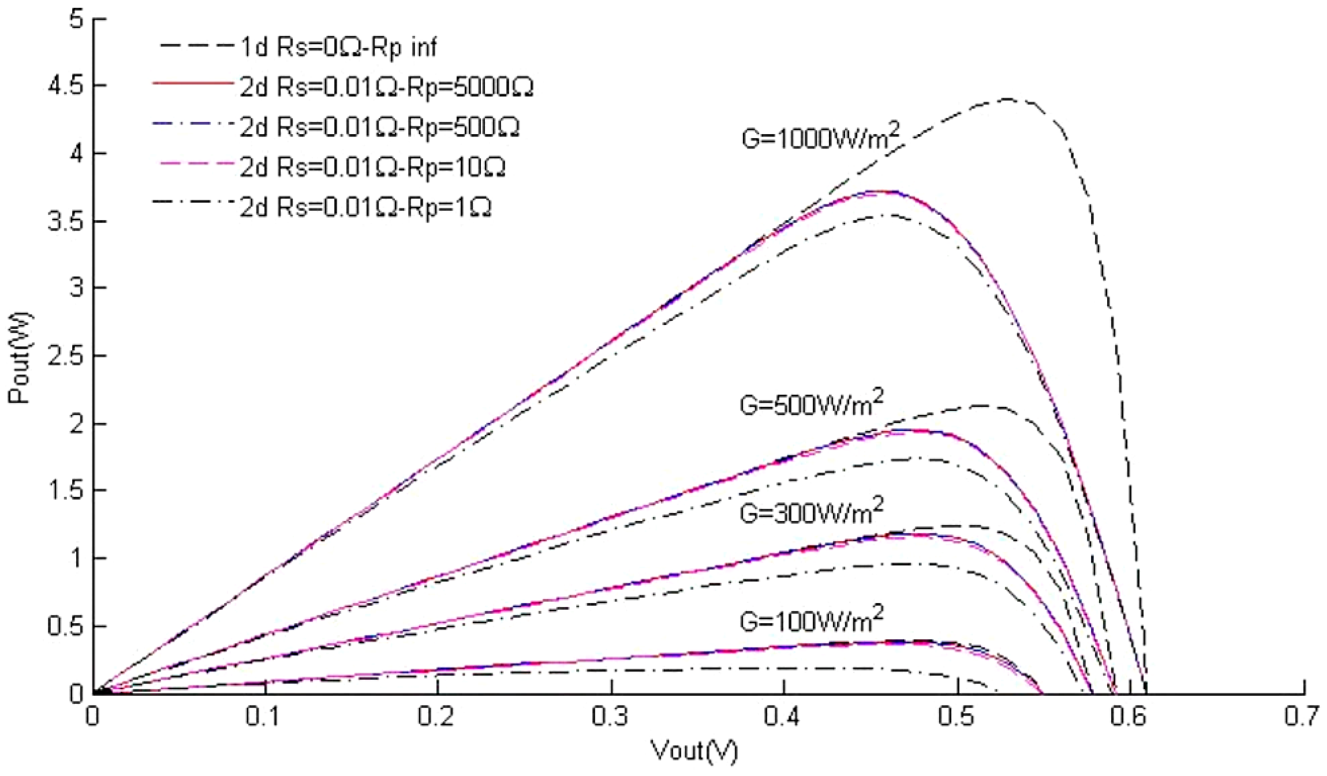
The incorporation of the parallel resistance Rp completes the number of variables that characterize the equivalent circuit of two diodes. Similarly to what was done with the equivalent representation of a diode, the importance of this resistive loss in the formation of the typical curves was examined, giving natural attention to the maximum power point. The structure was simulated with five different Rp values, exposed to progressively higher levels of solar radiation, between the 100 W/m2 and 1000 W/m2. Figure 9 and Figure 10 show the generated curves.
In both a diode structure and a two-diode structure, the leakage current through Rp is very small if the resistance is simulated with 5000 Ω—from this value the parallel branch approaches an infinite resistance. Then, since the resistances of 10 Ω and 200 Ω lead to characteristic curves identical to those found with 5000 Ω, it can be stated that Rp is negligible if its value is equal to or greater than 10 Ω. The same is no longer true with Rp reduced to 1 Ω. The current I starts to decrease to values close to the short-circuit voltage instead of remaining constant until the measurements of the maximum power electrical coordinates.
4.2. Characteristic Curves as a Function of Temperature and Parallel Resistance Rp
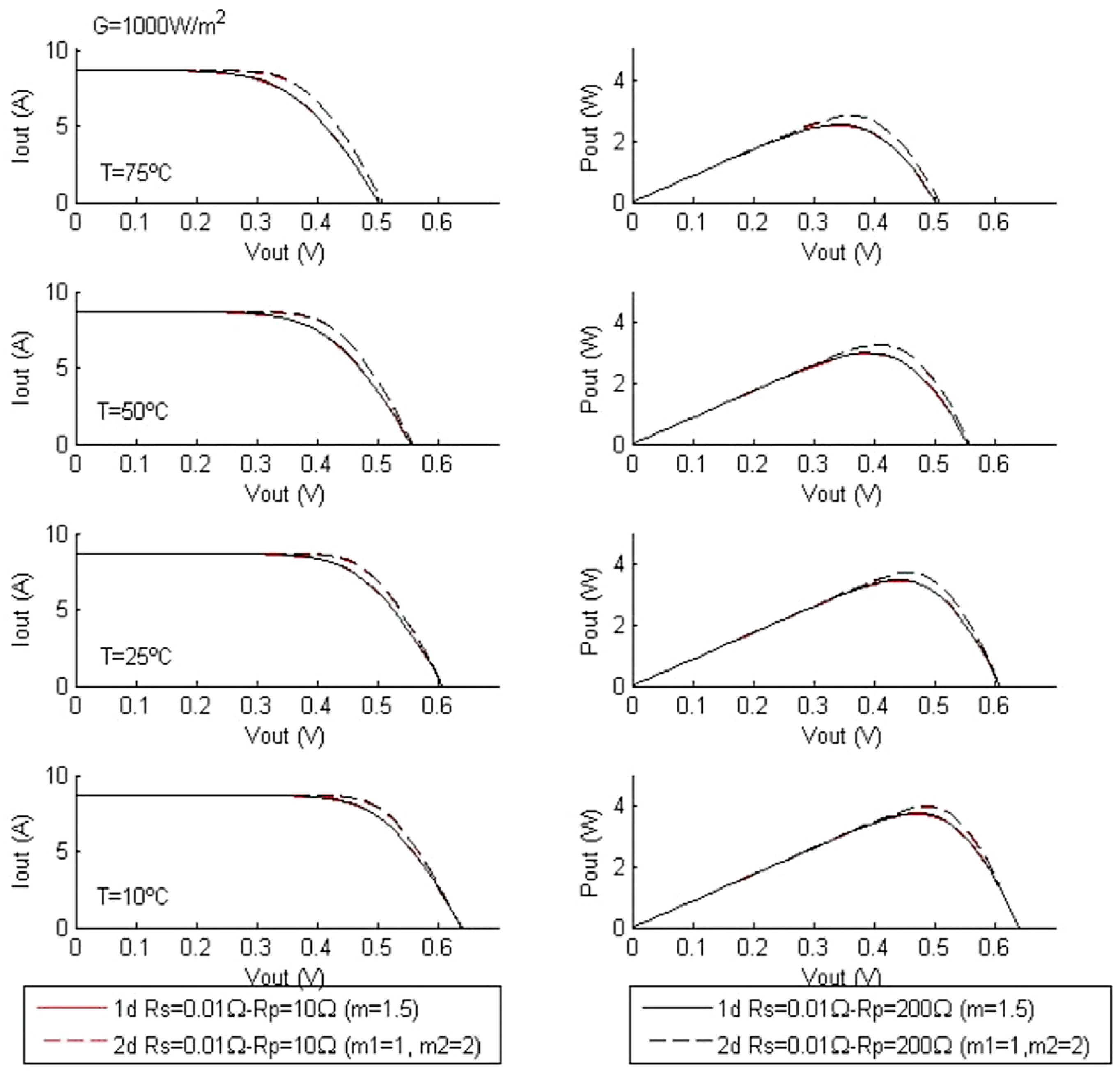
In this section, the evolution of the curves as a function of Rp (10 Ω and 200 Ω) is analyzed. The series resistance is equal and constant in both models. The parameters m, m1, and m2 are initialized with 1.5, 1, and 2, respectively. The simulation was carried out with three scenarios of solar radiation with 100 W/m2, 500 W/m2 and 1000 W/m2, respectively, and each with four levels of temperature, (10 °C, 25 °C, 50 °C, and 75 °C). The results can be witnessed in Figure 11, Figure 12 and Figure 13.
With solar power at 1000 W/m2 the open circuit voltage does not show any deviation between the two models. The same does not happen with 100 W/m2 and 500 W/m2 aggravating with the decrease of incident solar exposure. As for maximum power, the two-diode model is always at an advantage whatever the scenario. The difference is visible between 100 W/m2 and 500 W/m2, with a tendency to increase in the downward direction of the sun exposure. Over the same range of solar radiation, the temperature tends to maintain the constant difference.
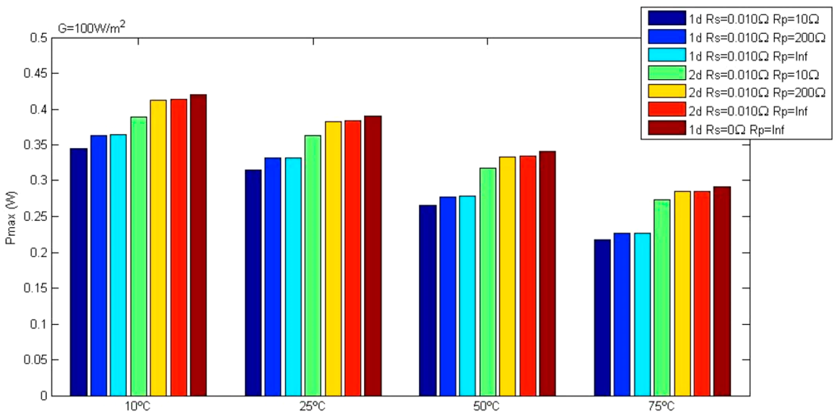
4.3. Comparative Table of Peak Power in the Set of Models
In order to support the conclusions concerning the role played by the parallel resistance in the one diode and two diode models, the data referring to the maximum power were agglutinated. The results are organized according to three solar power levels and by test temperature families and can be observed in Figure 14, Figure 15 and Figure 16.
From the analysis of Figure 14, Figure 15 and Figure 16 several conclusions can be assessed. At maximum or half solar exposure, both models lead to maximum values very close to the estimated power at infinite Rp. This trend remains with the temperature varying between 10 °C and 75 °C. Decreasing the light exposure to one tenth shows a significant deviation in any of the models with the Rp reduced to 10 Ω. The two-diode equivalent circuit is in any case more generous at peak power. The power deficit between the one-diode model versus the two-diode model is constant over the entire temperature range for the same level of radiation. However, it tends to worsen with the weakening of the incidence variable. The two-diode model tends to approximate the ideal one-diode model with the progressive reduction of incident radiation. With the limited incidence at 100 W/m2 the equivalent circuit performance (Rs = 10 mΩ and Rp = 200 Ω) is comparable, as it can be observed in Figure 16.
5. Conclusions
In this paper the equivalent electrical circuits used in the modeling of non-organic photovoltaic cells was presented, paying particular attention to the modeling of silicon-made cells. Two equivalent circuits of models were analyzed and then compared with the ideal model of the PV cell. The first equivalent circuit consists of the model of one diode, the second equivalent circuit of two diodes. The results show that the two-diode equivalent circuit is more advanced than the diode circuit in modeling an internal leakage current. The second diode fulfills this role by describing the additional losses, associated with the recombination of carriers in the depletion layer. The results firmly reveal that the five-parameter model is more penalized with the decrease in radiation than the seven-parameter counterpart. The same trend was observed with the rise in temperature. With a meteorological frame characterized by 1000 W/m2 of radiation and 10 °C of temperature, the deviation approaches 6.1%. By reducing the exposure to one-tenth the deviation reaches 12%. At the other end of the temperature range, the deviation reaches 10.4% at full sun exposure, and worsens up to 20.3% with exposure limited to the maximum. The most important contribution deduced form this study is that the two-diode model tends to approximate to the ideal PV cell model (one-diode model) with the progressive reduction of incident radiation. With the incidence limited to 100 W/m2 the equivalent circuit performance (Rs = 10 mΩ and Rp = 200 Ω) is almost identical to the ideal one-diode model. This means that, for regions were the solar incident radiation is lower, the ideal one-diode model behaves similarly to the more complex seven parameter equivalent circuit, thus allowing the user to opt for this circuit in detriment to the other more complex one which allows using a less complex software tool.
Author Contributions
E.M.G.R. performed the writing and original draft preparation and performed parts of the literature review. R.G. handled the writing and editing of the manuscript and contributed with parts of the literature review. M.M. and E.P. supervised, revised, and corrected the manuscript.
Funding
The current study was funded by Fundação para a Ciência e Tecnologia (FCT), under project UID/EMS/00151/2013 C-MAST, with reference POCI-01-0145-FEDER-007718.
Conflicts of Interest
The authors declare no conflict of interest.
References
- Cucchiella, F.; D’Adamo, I.; Gastaldi, M. Economic Analysis of a Photovoltaic System: A Resource for Residential Households. Energies 2017, 10, 814. [Google Scholar] [CrossRef]
- Sansaniwal, S.K.; Sharma, V.; Mathur, J. Energy and exergy analyses of various typical solar energy applications: A comprehensive review. Renew. Sustain. Energy Rev. 2018, 82, 1576–1601. [Google Scholar] [CrossRef]
- Li, Q.; Liu, Y.; Guo, S.; Zhou, H. Solar energy storage in the rechargeable batteries. Nano Today 2017, 16, 46–60. [Google Scholar] [CrossRef]
- Teo, J.C.; Tan, R.H.G.; Mok, V.H.; Ramachandaramurthy, V.K.; Tan, C. Impact of Partial Shading on the P-V Characteristics and the Maximum Power of a Photovoltaic String. Energies 2018, 11, 1860. [Google Scholar] [CrossRef]
- Jacobi, N.; Haas, W.; Wiedenhofer, D.; Mayer, A. Providing an economy-wide monitoring framework for the circular economy in Austria: Status quo and challenges. Resour. Conserv. Recycl. 2018, 137, 156–166. [Google Scholar] [CrossRef]
- Yousif, J.; Kazem, H.; Boland, J. Predictive Models for Photovoltaic Electricity Production in Hot Weather Conditions. Energies 2017, 10, 971. [Google Scholar] [CrossRef]
- Chang, B.; Starcher, K. Evaluation of Wind and Solar Energy Investments in Texas. Renew. Energy 2018. [Google Scholar] [CrossRef]
- Gimeno, J.Á.; Llera, E.; Scarpellini, S. Investment Determinants in Self-Consumption Facilities: Characterization and Qualitative Analysis in Spain. Energies 2018, 11, 2178. [Google Scholar] [CrossRef]
- Beránek, V.; Olšan, T.; Libra, M.; Poulek, V.; Sedláček, J.; Dang, M.-Q.; Tyukhov, I. New Monitoring System for Photovoltaic Power Plants’ Management. Energies 2018, 11, 2495. [Google Scholar] [CrossRef]
- Gelsor, N.; Gelsor, N.; Wangmo, T.; Chen, Y.-C.; Frette, Ø.; Stamnes, J.J.; Hamre, B. Solar energy on the Tibetan Plateau: Atmospheric influences. Sol. Energy 2018, 173, 984–992. [Google Scholar] [CrossRef]
- Todde, G.; Murgia, L.; Carrelo, I.; Hogan, R.; Pazzona, A.; Ledda, L.; Narvarte, L. Embodied Energy and Environmental Impact of Large-Power Stand-Alone Photovoltaic Irrigation Systems. Energies 2018, 11, 2110. [Google Scholar] [CrossRef]
- Huang, Y.-P.; Ye, C.-E.; Chen, X. A Modified Firefly Algorithm with Rapid Response Maximum Power Point Tracking for Photovoltaic Systems under Partial Shading Conditions. Energies 2018, 11, 2284. [Google Scholar] [CrossRef]
- Merzifonluoglu, Y.; Uzgoren, E. Photovoltaic power plant design considering multiple uncertainties and risk. Ann. Oper. Res. 2018, 262, 153–184. [Google Scholar] [CrossRef]
- Shah, S.W.A.; Mahmood, M.N.; Das, N. Strategic asset management framework for the improvement of large scale PV power plants in Australia. In Proceedings of the 2016 Australasian Universities Power Engineering Conference (AUPEC), Brisbane, QLD, Australia, 25–28 September 2016; pp. 1–5. [Google Scholar]
- Arefifar, S.A.; Paz, F.; Ordonez, M. Improving Solar Power PV Plants Using Multivariate Design Optimization. IEEE J. Emerg. Sel. Top. Power Electron. 2017, 5, 638–650. [Google Scholar] [CrossRef]
- Peng, Z.; Herfatmanesh, M.R.; Liu, Y. Cooled solar PV panels for output energy efficiency optimisation. Energy Convers. Manag. 2017, 150, 949–955. [Google Scholar] [CrossRef]
- Elibol, E.; Özmen, Ö.T.; Tutkun, N.; Köysal, O. Outdoor performance analysis of different PV panel types. Renew. Sustain. Energy Rev. 2017, 67, 651–661. [Google Scholar] [CrossRef]
- Zhou, Z.; Macaulay, J. An Emulated PV Source Based on an Unilluminated Solar Panel and DC Power Supply. Energies 2017, 10, 2075. [Google Scholar] [CrossRef]
- Seyedmahmoudian, M.; Horan, B.; Rahmani, R.; Maung Than Oo, A.; Stojcevski, A. Efficient Photovoltaic System Maximum Power Point Tracking Using a New Technique. Energies 2016, 9, 147. [Google Scholar] [CrossRef]
- Wang, F.; Wu, X.; Lee, F.C.; Wang, Z.; Kong, P.; Zhuo, F. Analysis of Unified Output MPPT Control in Subpanel PV Converter System. IEEE Trans. Power Electron. 2014, 29, 1275–1284. [Google Scholar] [CrossRef]
- Wang, Z.; Das, N.; Helwig, A.; Ahfock, T. Modeling of multi-junction solar cells for maximum power point tracking to improve the conversion efficiency. In Proceedings of the 2017 Australasian Universities Power Engineering Conference (AUPEC), Melbourne, VIC, Australia, 19–22 November 2017; pp. 1–6. [Google Scholar]
- Das, N.; Wongsodihardjo, H.; Islam, S. A Preliminary Study on Conversion Efficiency Improvement of a Multi-junction PV Cell with MPPT. In Smart Power Systems and Renewable Energy System Integration; Jayaweera, D., Ed.; Studies in Systems, Decision and Control; Springer International Publishing: Cham, Switzerland, 2016; pp. 49–73. ISBN 978-3-319-30427-4. [Google Scholar]
- Das, N.; Wongsodihardjo, H.; Islam, S. Modeling of multi-junction photovoltaic cell using MATLAB/Simulink to improve the conversion efficiency. Renew. Energy 2015, 74, 917–924. [Google Scholar] [CrossRef]
- Das, N.; Ghadeer, A.A.; Islam, S. Modelling and analysis of multi-junction solar cells to improve the conversion efficiency of photovoltaic systems. In Proceedings of the 2014 Australasian Universities Power Engineering Conference (AUPEC), Perth, WA, Australia, 28 September–1 October 2014; pp. 1–5. [Google Scholar]
- Jin, Y.; Hou, W.; Li, G.; Chen, X. A Glowworm Swarm Optimization-Based Maximum Power Point Tracking for Photovoltaic/Thermal Systems under Non-Uniform Solar Irradiation and Temperature Distribution. Energies 2017, 10, 541. [Google Scholar] [CrossRef]
- Zhao, J.; Zhou, X.; Ma, Y.; Liu, Y. Analysis of Dynamic Characteristic for Solar Arrays in Series and Global Maximum Power Point Tracking Based on Optimal Initial Value Incremental Conductance Strategy under Partially Shaded Conditions. Energies 2017, 10, 120. [Google Scholar] [CrossRef]
- Tobón, A.; Peláez-Restrepo, J.; Villegas-Ceballos, J.P.; Serna-Garcés, S.I.; Herrera, J.; Ibeas, A. Maximum Power Point Tracking of Photovoltaic Panels by Using Improved Pattern Search Methods. Energies 2017, 10, 1316. [Google Scholar] [CrossRef]
- Hadji, S.; Gaubert, J.-P.; Krim, F. Real-Time Genetic Algorithms-Based MPPT: Study and Comparison (Theoretical an Experimental) with Conventional Methods. Energies 2018, 11, 459. [Google Scholar] [CrossRef]
- Cubas, J.; Pindado, S.; de Manuel, C. Explicit Expressions for Solar Panel Equivalent Circuit Parameters Based on Analytical Formulation and the Lambert W-Function. Energies 2014, 7, 4098–4115. [Google Scholar] [CrossRef] [Green Version]
- Bahrami, M.; Gavagsaz-Ghoachani, R.; Zandi, M.; Phattanasak, M.; Maranzanaa, G.; Nahid-Mobarakeh, B.; Pierfederici, S.; Meibody-Tabar, F. Hybrid maximum power point tracking algorithm with improved dynamic performance. Renew. Energy 2019, 130, 982–991. [Google Scholar] [CrossRef]
- Rodrigues, E.M.G.; Melício, R.; Mendes, V.M.F.; Catalão, J.P.S. Simulation of a Solar Cell Considering Single-diode Equivalent Circuit Model. Renew. Energy Power Qual. J. 2011, 1, 369–373. [Google Scholar] [CrossRef]
- Rodrigues, E.M.G.; Godina, R.; Pouresmaeil, E.; Catalão, J.P.S. Simulation study of a photovoltaic cell with increasing levels of model complexity. In Proceedings of the 2017 IEEE International Conference on Environment and Electrical Engineering and 2017 IEEE Industrial and Commercial Power Systems Europe (EEEIC/I CPS Europe), Milan, Italy, 6–9 June 2017; pp. 1–5. [Google Scholar]
- Villalva, M.G.; Gazoli, J.R.; Filho, E.R. Comprehensive Approach to Modeling and Simulation of Photovoltaic Arrays. IEEE Trans. Power Electron. 2009, 24, 1198–1208. [Google Scholar] [CrossRef]
- Carrero, C.; Amador, J.; Arnaltes, S. A single procedure for helping PV designers to select silicon PV modules and evaluate the loss resistances. Renew. Energy 2007, 32, 2579–2589. [Google Scholar] [CrossRef]
- Rodriguez, C.; Amaratunga, G.A.J. Analytic Solution to the Photovoltaic Maximum Power Point Problem. IEEE Trans. Circuits Syst. Regul. Pap. 2007, 54, 2054–2060. [Google Scholar] [CrossRef]
- Patel, H.; Agarwal, V. MATLAB-Based Modeling to Study the Effects of Partial Shading on PV Array Characteristics. IEEE Trans. Energy Convers. 2008, 23, 302–310. [Google Scholar] [CrossRef]
- Ahmed, S.S.; Mohsin, M. Analytical Determination of the Control Parameters for a Large Photovoltaic Generator Embedded in a Grid System. IEEE Trans. Sustain. Energy 2011, 2, 122–130. [Google Scholar] [CrossRef]
- Kim, I.; Kim, M.; Youn, M. New Maximum Power Point Tracker Using Sliding-Mode Observer for Estimation of Solar Array Current in the Grid-Connected Photovoltaic System. IEEE Trans. Ind. Electron. 2006, 53, 1027–1035. [Google Scholar] [CrossRef]
- Xiao, W.; Dunford, W.G.; Capel, A. A novel modeling method for photovoltaic cells. In Proceedings of the 2004 IEEE 35th Annual Power Electronics Specialists Conference (IEEE Cat. No. 04CH37551), Aachen, Germany, 20–25 June 2004; Volume 3, pp. 1950–1956. [Google Scholar]
- Yusof, Y.; Sayuti, S.H.; Latif, M.A.; Wanik, M.Z.C. Modeling and simulation of maximum power point tracker for photovoltaic system. In Proceedings of the PECon 2004 National Power and Energy Conference, Kuala Lumpur, Malaysia, 29–30 November 2004; pp. 88–93. [Google Scholar]
- Khouzam, K.; Ly, C.; Koh, C.K.; Ng, P.Y. Simulation and real-time modelling of space photovoltaic systems. In Proceedings of the 1994 IEEE 1st World Conference on Photovoltaic Energy Conversion—WCPEC (A Joint Conference of PVSC, PVSEC and PSEC), Waikoloa, HI, USA, 5–9 December 1994; Volume 2, pp. 2038–2041. [Google Scholar]
- Glass, M.C. Improved solar array power point model with SPICE realization. In Proceedings of the 31st Intersociety Energy Conversion Engineering Conference, Washington, DC, USA, 11–16 August 1996; Volume 1, pp. 286–291. [Google Scholar]
- Altas, I.H.; Sharaf, A.M. A Photovoltaic Array Simulation Model for Matlab-Simulink GUI Environment. In Proceedings of the 2007 International Conference on Clean Electrical Power, Capri, Itlay, 21–23 May 2007; pp. 341–345. [Google Scholar]
- Matagne, E.; Chenni, R.; Bachtiri, R.E. A photovoltaic cell model based on nominal data only. In Proceedings of the 2007 International Conference on Power Engineering, Energy and Electrical Drives, Setubal, Portugal, 12–14 April 2007; pp. 562–565. [Google Scholar]
- Tan, Y.T.; Kirschen, D.S.; Jenkins, N. A model of PV generation suitable for stability analysis. IEEE Trans. Energy Convers. 2004, 19, 748–755. [Google Scholar] [CrossRef]
- Kajihara, A.; Harakawa, A.T. Model of photovoltaic cell circuits under partial shading. In Proceedings of the 2005 IEEE International Conference on Industrial Technology, Hong Kong, China, 14–17 December 2005; pp. 866–870. [Google Scholar]
- Benavides, N.D.; Chapman, P.L. Modeling the effect of voltage ripple on the power output of photovoltaic modules. IEEE Trans. Ind. Electron. 2008, 55, 2638–2643. [Google Scholar] [CrossRef]
- Sera, D. Real-Time Modelling, Diagnostics and Optimised MPPT for Residential PV Systems; Institut for Energiteknik, Aalborg Universitet: Aalborg, Denmark, 2009; ISBN 978-87-89179-76-6. [Google Scholar]
- Bashirov, A. Transcendental Functions. In Mathematical Analysis Fundamentals; Bashirov, A., Ed.; Elsevier: Boston, MA, USA, 2014; Chapter 11; pp. 253–305. ISBN 978-0-12-801001-3. [Google Scholar]
- Danandeh, M.A.; Mousavi, G.S.M. Comparative and comprehensive review of maximum power point tracking methods for PV cells. Renew. Sustain. Energy Rev. 2018, 82, 2743–2767. [Google Scholar] [CrossRef]
- Batarseh, M.G.; Za’ter, M.E. Hybrid maximum power point tracking techniques: A comparative survey, suggested classification and uninvestigated combinations. Sol. Energy 2018, 169, 535–555. [Google Scholar] [CrossRef]
- Uoya, M.; Koizumi, H. A Calculation Method of Photovoltaic Array’s Operating Point for MPPT Evaluation Based on One-Dimensional Newton–Raphson Method. IEEE Trans. Ind. Appl. 2015, 51, 567–575. [Google Scholar] [CrossRef]
- Gow, J.A.; Manning, C.D. Development of a photovoltaic array model for use in power-electronics simulation studies. IEE Proc.—Electr. Power Appl. 1999, 146, 193–200. [Google Scholar] [CrossRef]
- Walker, G.R. Evaluating MPPT converter topologies using a Matlab PV model. Aust. J. Electr. Electron. Eng. 2001, 21, 49–55. [Google Scholar]
- Ishaque, K.; Salam, Z.; Taheri, H. Simple, fast and accurate two-diode model for photovoltaic modules. Sol. Energy Mater. Sol. Cells 2011, 95, 586–594. [Google Scholar] [CrossRef]
- Nishioka, K.; Sakitani, N.; Uraoka, Y.; Fuyuki, T. Analysis of multicrystalline silicon solar cells by modified 3-diode equivalent circuit model taking leakage current through periphery into consideration. Sol. Energy Mater. Sol. Cells 2007, 91, 1222–1227. [Google Scholar] [CrossRef]
- Enrique, J.M.; Durán, E.; Sidrach-de-Cardona, M.; Andújar, J.M. Theoretical assessment of the maximum power point tracking efficiency of photovoltaic facilities with different converter topologies. Sol. Energy 2007, 81, 31–38. [Google Scholar] [CrossRef]
- Chowdhury, S.; Chowdhury, S.P.; Taylor, G.A.; Song, Y.H. Mathematical modelling and performance evaluation of a stand-alone polycrystalline PV plant with MPPT facility. In Proceedings of the 2008 IEEE Power and Energy Society General Meeting—Conversion and Delivery of Electrical Energy in the 21st Century, Pittsburgh, PA, USA, 20–24 July 2008; pp. 1–7. [Google Scholar]
- Salam, Z.; Ishaque, K.; Taheri, H. An improved two-diode photovoltaic (PV) model for PV system. In Proceedings of the 2010 Joint International Conference on Power Electronics, Drives and Energy Systems 2010 Power, New Delhi, India, 20–23 December 2010; pp. 1–5. [Google Scholar]
- Gow, J.A.; Manning, C.D. Development of a model for photovoltaic arrays suitable for use in simulation studies of solar energy conversion systems. In Proceedings of the 1996 Sixth International Conference on Power Electronics and Variable Speed Drives, Nottingham, UK, 23–25 September 1996; pp. 69–74. [Google Scholar]
- Hyvarinen, J.; Karila, J. New analysis method for crystalline silicon cells. In Proceedings of the 3rd World Conference on Photovoltaic Energy Conversion, Osaka, Japan, 1–18 May 2003; Volume 2, pp. 1521–1524. [Google Scholar]
- Bowden, S.; Rohatgi, A. Rapid and Accurate Determination of Series Resistance and Fill Factor Losses in Industrial Silicon Solar Cells. In Proceedings of the 17th European Photovoltaic Solar Energy Conference, Munich, Germany, 22–26 October 2001. [Google Scholar]
- Sandrolini, L.; Artioli, M.; Reggiani, U. Numerical method for the extraction of photovoltaic module double-diode model parameters through cluster analysis. Appl. Energy 2010, 87, 442–451. [Google Scholar] [CrossRef]
- Dolan, J.A.; Lee, R.; Yeh, Y.; Yeh, C.; Nguyen, D.Y.; Ben-Menahem, S.; Ishihara, A.K. Neural network estimation of photovoltaic I–V curves under partially shaded conditions. In Proceedings of the 2011 International Joint Conference on Neural Networks, San Jose, CA, USA, 31 July–5 August 2011; pp. 1358–1365. [Google Scholar]
- Ishaque, K.; Salam, Z.; Taheri, H.; Shamsudin, A. A critical evaluation of EA computational methods for Photovoltaic cell parameter extraction based on two diode model. Sol. Energy 2011, 85, 1768–1779. [Google Scholar] [CrossRef]
Figure 1.
Five-parameter equivalent electric circuit of the photovoltaic (PV) module.
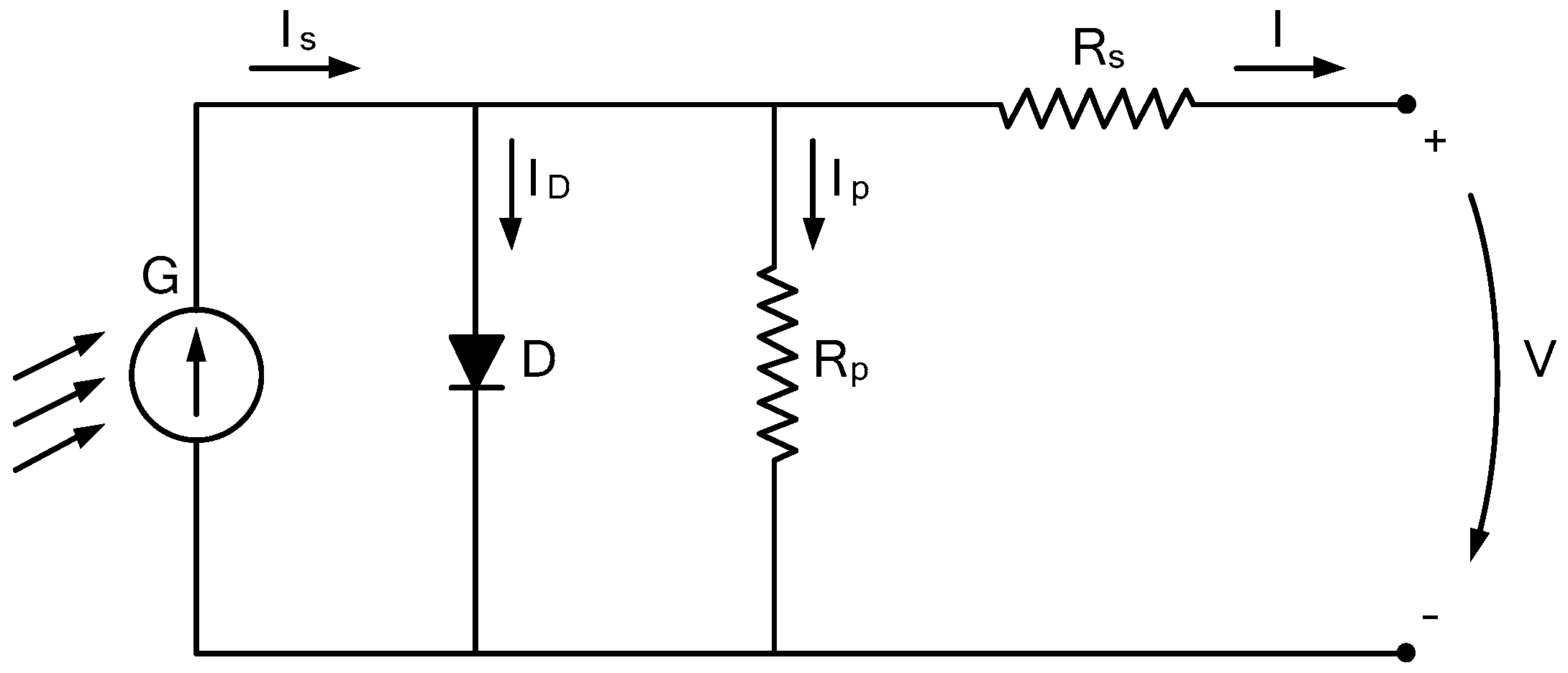
Figure 2.
I-V curves as a function of the parallel resistance Rp and with Rs: (a) 0 Ω and (b) 10 mΩ; (STC).
Figure 2.
I-V curves as a function of the parallel resistance Rp and with Rs: (a) 0 Ω and (b) 10 mΩ; (STC).

Figure 3.
Extended I-V characteristic curves.
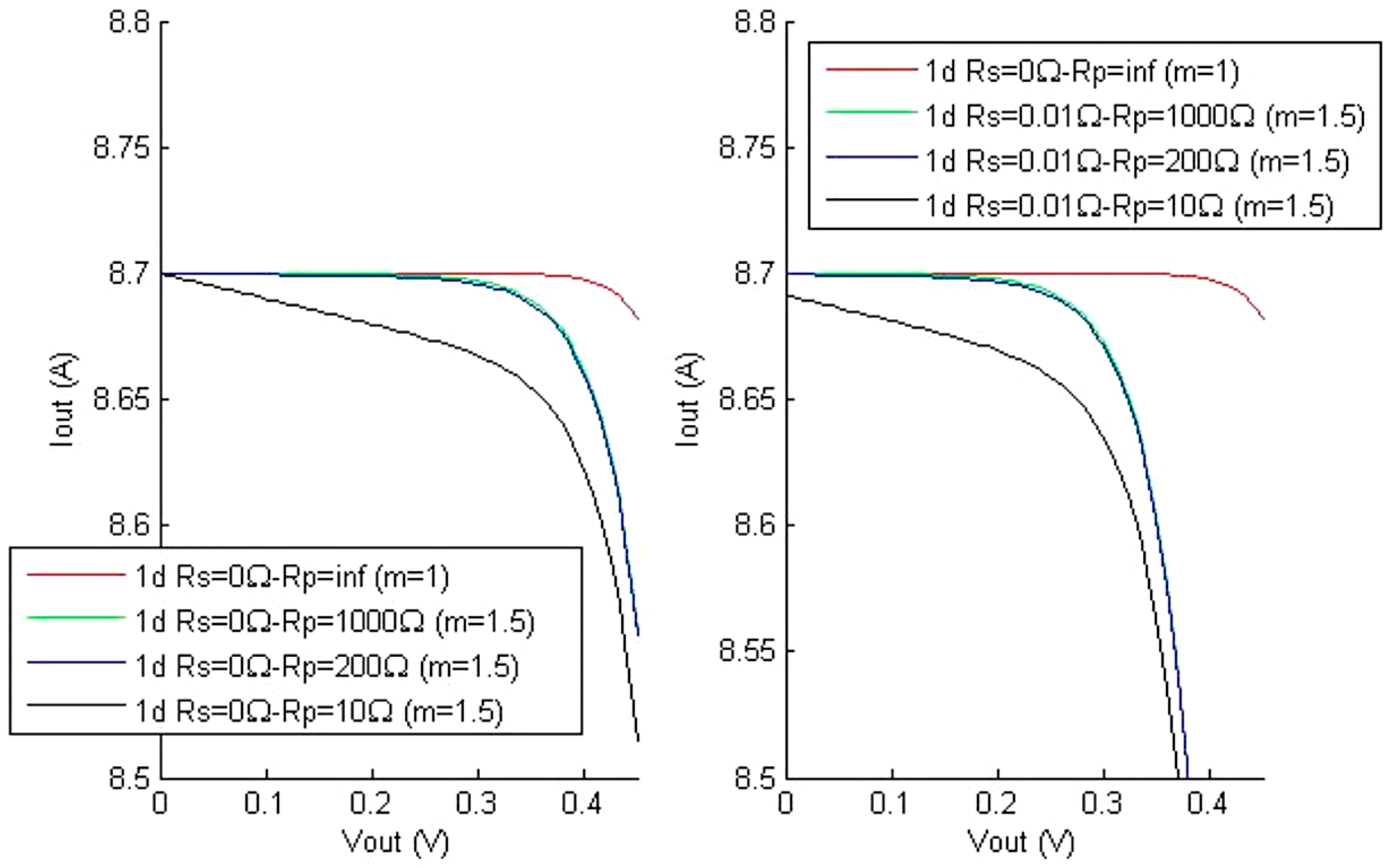
Figure 4.
P-V curves as a function of the parallel resistance Rp and with Rs: (a) 0 Ω and (b) 10 mΩ; (STC).
Figure 4.
P-V curves as a function of the parallel resistance Rp and with Rs: (a) 0 Ω and (b) 10 mΩ; (STC).

Figure 5.
Characteristic curves in function of temperature and parallel resistance Rp, with a constant resistance Rs (G = 1000 W/m2).
Figure 5.
Characteristic curves in function of temperature and parallel resistance Rp, with a constant resistance Rs (G = 1000 W/m2).

Figure 6.
Characteristic curves in function of temperature and parallel resistance Rp, with a constant resistance Rs (G = 500 W/m2).
Figure 6.
Characteristic curves in function of temperature and parallel resistance Rp, with a constant resistance Rs (G = 500 W/m2).

Figure 7.
Characteristic curves in function of temperature and parallel resistance Rp, with a constant resistance Rs (G = 100 W/m2).
Figure 7.
Characteristic curves in function of temperature and parallel resistance Rp, with a constant resistance Rs (G = 100 W/m2).

Figure 8.
Seven-parameter equivalent electric circuit of the photovoltaic (PV) module.

Figure 9.
I-V curves of equivalent 1 and 2 diode circuits in function of the solar radiation and of the parallel resistance Rp, with series resistance Rs constant (T = 25 °C).
Figure 9.
I-V curves of equivalent 1 and 2 diode circuits in function of the solar radiation and of the parallel resistance Rp, with series resistance Rs constant (T = 25 °C).

Figure 10.
P-V curves of equivalent 1 and 2 diode circuits in function of the solar radiation and of the parallel resistance Rp, with series resistance Rs constant (T = 25 °C).
Figure 10.
P-V curves of equivalent 1 and 2 diode circuits in function of the solar radiation and of the parallel resistance Rp, with series resistance Rs constant (T = 25 °C).

Figure 11.
Characteristic curves of equivalent circuits of one and two diodes in function of temperature and parallel resistance Rp, with a constant resistance Rs (G = 1000 W/m2).
Figure 11.
Characteristic curves of equivalent circuits of one and two diodes in function of temperature and parallel resistance Rp, with a constant resistance Rs (G = 1000 W/m2).

Figure 12.
Characteristic curves of equivalent circuits of one and two diodes in function of temperature and parallel resistance Rp, with a constant resistance Rs (G = 500 W/m2).
Figure 12.
Characteristic curves of equivalent circuits of one and two diodes in function of temperature and parallel resistance Rp, with a constant resistance Rs (G = 500 W/m2).
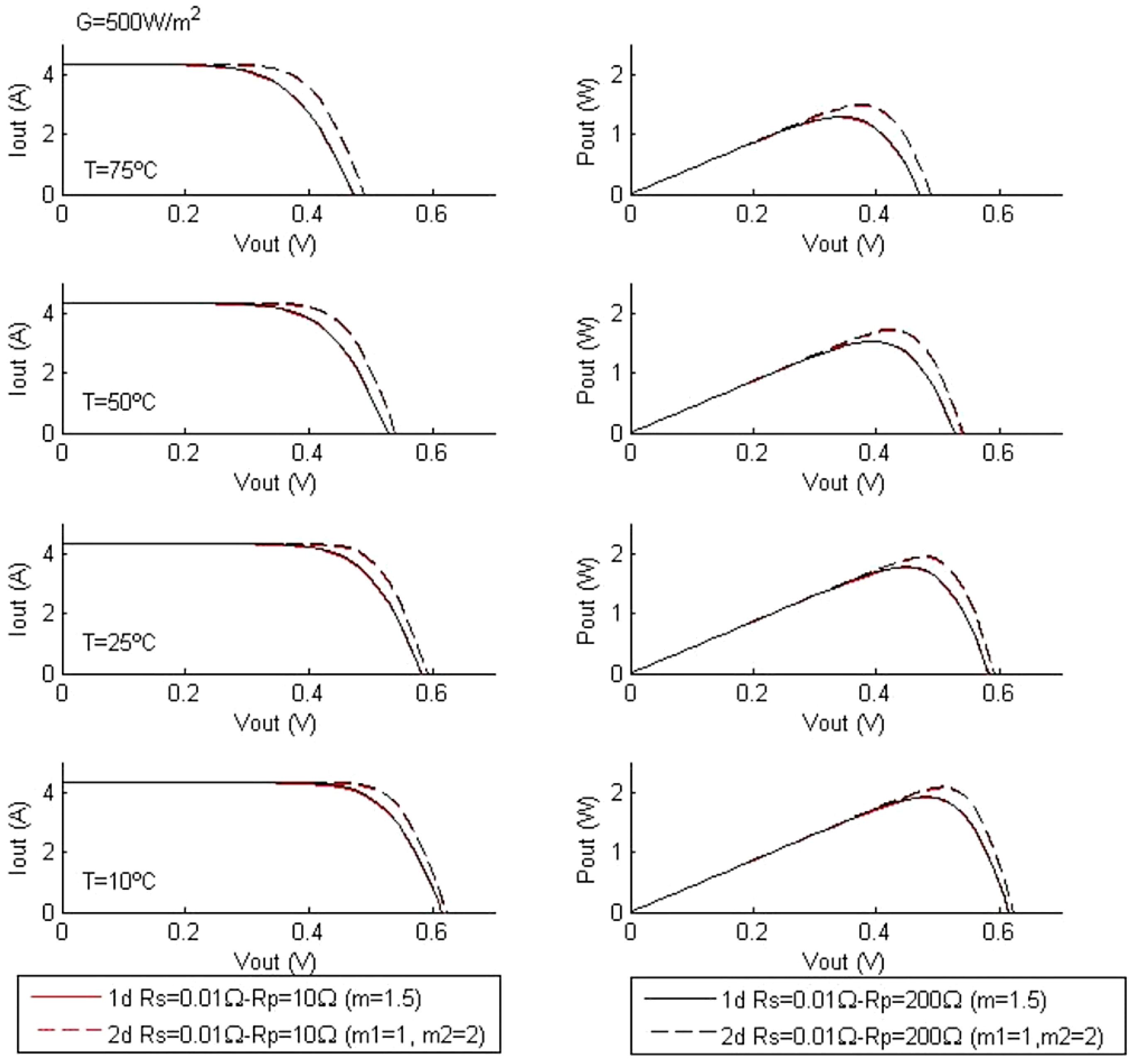
Figure 13.
Characteristic curves of equivalent circuits of one and two diodes in function of temperature and parallel resistance Rp, with a constant resistance Rs (G = 100 W/m2).
Figure 13.
Characteristic curves of equivalent circuits of one and two diodes in function of temperature and parallel resistance Rp, with a constant resistance Rs (G = 100 W/m2).
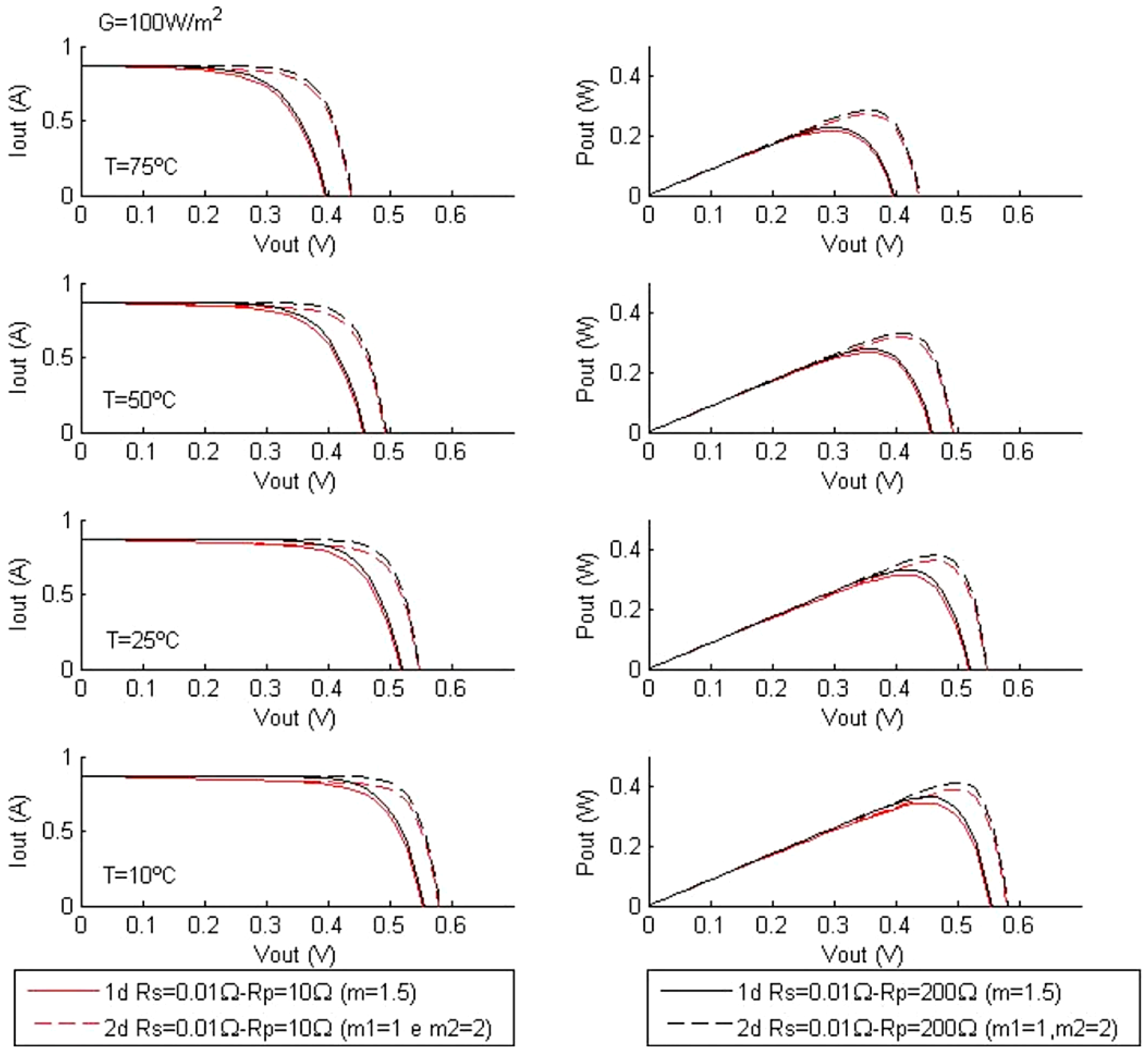
Figure 14.
Maximum power as a function of temperature (G = 1000 W/m2).
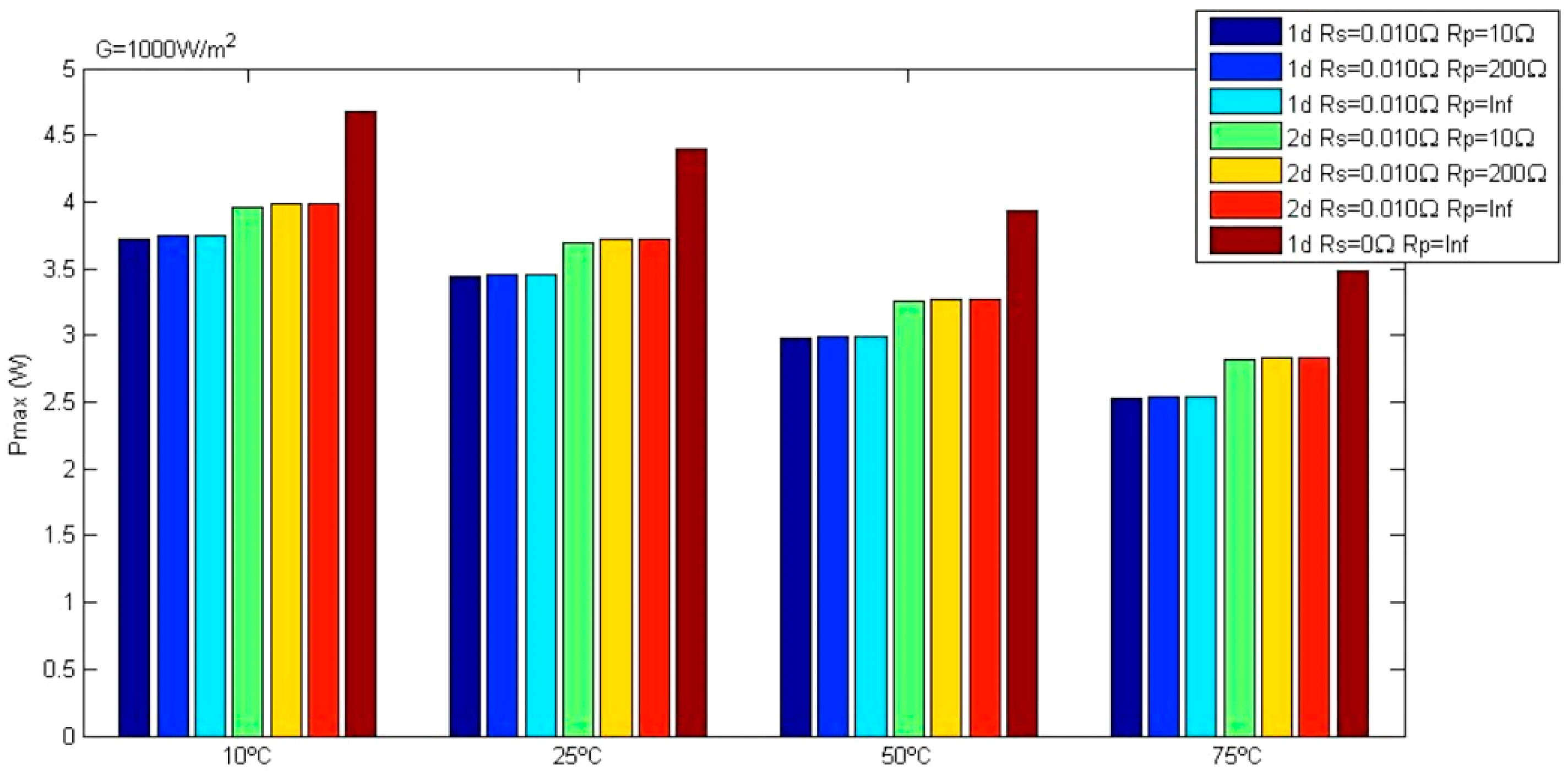
Figure 15.
Maximum power as a function of temperature (G = 500 W/m2).
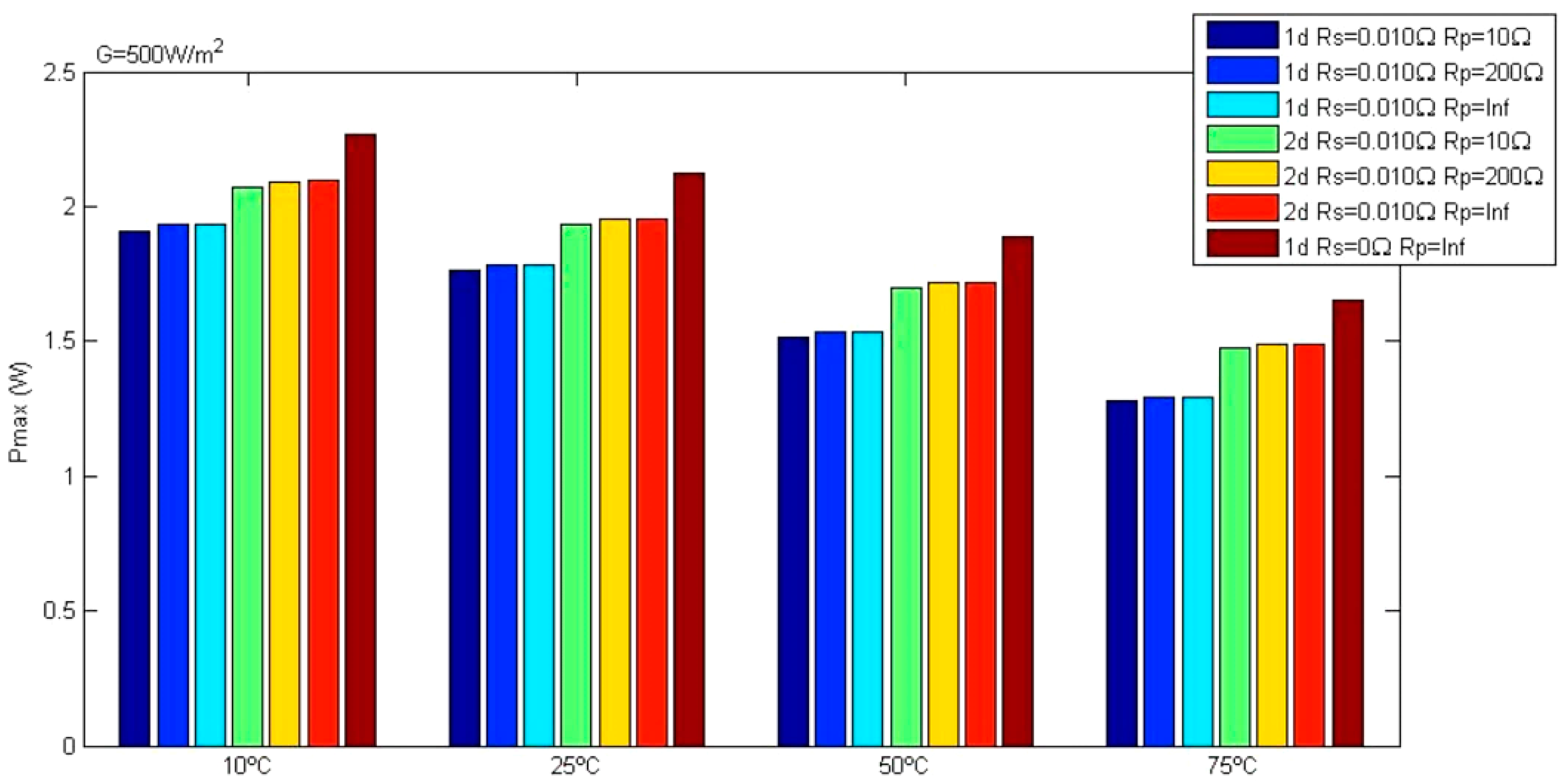
Figure 16.
Maximum power as a function of temperature (G = 100 W/m2).
© 2018 by the authors. Licensee MDPI, Basel, Switzerland. This article is an open access article distributed under the terms and conditions of the Creative Commons Attribution (CC BY) license (http://creativecommons.org/licenses/by/4.0/).
Share and Cite
MDPI and ACS Style
Manuel Godinho Rodrigues, E.; Godina, R.; Marzband, M.; Pouresmaeil, E. Simulation and Comparison of Mathematical Models of PV Cells with Growing Levels of Complexity. Energies 2018, 11, 2902. https://doi.org/10.3390/en11112902
AMA Style
Manuel Godinho Rodrigues E, Godina R, Marzband M, Pouresmaeil E. Simulation and Comparison of Mathematical Models of PV Cells with Growing Levels of Complexity. Energies. 2018; 11(11):2902. https://doi.org/10.3390/en11112902
Chicago/Turabian StyleManuel Godinho Rodrigues, Eduardo, Radu Godina, Mousa Marzband, and Edris Pouresmaeil. 2018. "Simulation and Comparison of Mathematical Models of PV Cells with Growing Levels of Complexity" Energies 11, no. 11: 2902. https://doi.org/10.3390/en11112902
Note that from the first issue of 2016, this journal uses article numbers instead of page numbers. See further details here.