Coupling Methodology for Studying the Far Field Effects of Wave Energy Converter Arrays over a Varying Bathymetry


Department of Civil Engineering, Ghent University, Technologierpark 904, B-9052 Zwijnaarde, Belgium
*
Author to whom correspondence should be addressed.
Energies 2018, 11(11), 2899; https://doi.org/10.3390/en11112899
Submission received: 1 October 2018
/
Revised: 16 October 2018
/
Accepted: 18 October 2018
/
Published: 25 October 2018
(This article belongs to the Special Issue Offshore Renewable Energy: Ocean Waves, Tides and Offshore Wind)
Abstract
:For renewable wave energy to operate at grid scale, large arrays of Wave Energy Converters (WECs) need to be deployed in the ocean. Due to the hydrodynamic interactions between the individual WECs of an array, the overall power absorption and surrounding wave field will be affected, both close to the WECs (near field effects) and at large distances from their location (far field effects). Therefore, it is essential to model both the near field and far field effects of WEC arrays. It is difficult, however, to model both effects using a single numerical model that offers the desired accuracy at a reasonable computational time. The objective of this paper is to present a generic coupling methodology that will allow to model both effects accurately. The presented coupling methodology is exemplified using the mild slope wave propagation model MILDwave and the Boundary Elements Methods (BEM) solver NEMOH. NEMOH is used to model the near field effects while MILDwave is used to model the WEC array far field effects. The information between the two models is transferred using a one-way coupling. The results of the NEMOH-MILDwave coupled model are compared to the results from using only NEMOH for various test cases in uniform water depth. Additionally, the NEMOH-MILDwave coupled model is validated against available experimental wave data for a 9-WEC array. The coupling methodology proves to be a reliable numerical tool as the results demonstrate a difference between the numerical simulations results smaller than 5% and between the numerical simulations results and the experimental data ranging from 3% to 11%. The simulations are subsequently extended for a varying bathymetry, which will affect the far field effects. As a result, our coupled model proves to be a suitable numerical tool for simulating far field effects of WEC arrays for regular and irregular waves over a varying bathymetry.
1. Introduction
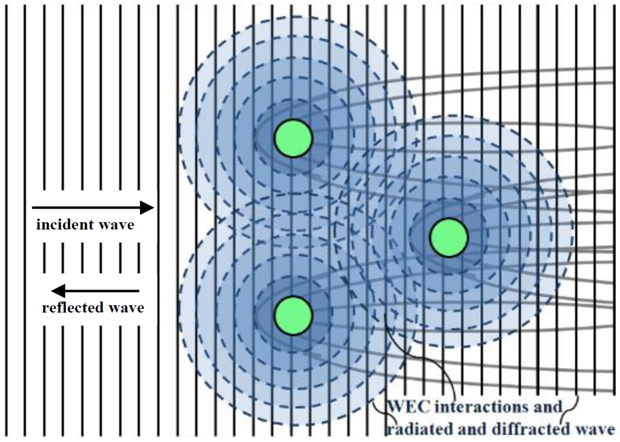
Wave energy is a renewable energy source with the potential to contribute to reduce the world’s dependency on fossil fuels. Compared to other renewable energy sources, such as wind and solar, wave energy conversion lacks technologic and economic development. In order for wave energy to be economically viable, large farms of Wave Energy Converters (WECs) have to be deployed at the same location, which will enable wave energy to operate at grid scale and compete with wind farms. This is usually termed as WEC arrays or WEC farms in literature. For this study, the term WEC farm refers to a scale comparable to a wind farm, while a WEC array is a small group of WECs closely spaced within the farm. Due to the hydrodynamic interactions between the individual WECs in the array, the overall power absorption will be affected. The hydrodynamic problem of power absorption is characterized by two different problems: the diffraction problem and the radiation problem. The diffraction problem studies the change in direction of the incident wave field due to the presence of the WECs. Assuming the WECs to be stationary and depending on their geometry, a diffracted wave field around the WECs can be obtained. The radiation problem refers to the generation of a radiated wave field around the WECs due to the oscillations of the bodies caused by the incident wave field. The superposition of the diffracted and radiated wave fields using linear wave theory results in a complex perturbed wave field around the WECs. This is often described as the near field effects in literature (illustrated in Figure 1). In addition, the absorption and redistribution of the wave energy around the WECs will also cause a wake behind the WEC array, which is an area of reduced wave height in the lee of the WECs. Wake effects can have a positive or negative impact on the coastline and other sea users. This is often described as the far field effect of WECs.
Substantial numerical research has been carried out to study the near field effects and interaction factors of WECs, to optimize the array lay-out for maximizing power output. To date, various wave-structure interaction models have been used: numerical array models based on semi-analytical coefficient calculation [2,3], Boundary Elements Methods (BEM) based on potential flow theory [4,5] and Computational Fluid Dynamics (CFD) [6].
Far field effects are traditionally studied using wave propagation models. In [7,8,9,10,11], phase-averaging spectral models are used to obtain the wave field in the lee of a WEC array. The WEC arrays in these studies are simplified as obstacles with a fixed transmission coefficient. In the same way, Ref. [12] used a time-dependent mild-slope equation model and simplified each WEC as a wave power absorbing obstacle. To obtain the absorption coefficient for phase-averaging spectral models and the wave power absorbing obstacle coefficient for time-dependent mild-slope equation models, tank testing or numerical modelling is required. Therefore, the modelling of the hydrodynamic interactions is not taken into account resulting in a simplified WEC parametrization, which leads to low accuracy results.
As pointed out in [13], the currently available approaches either focus on modelling the near field effects at high fidelity but with high computational cost or the far field effects with low fidelity but low computational cost, in part due to the limitation of modelling both effects simultaneously using a single solver. On the one hand, wave-structure interaction solvers require a long computational time, which increases exponentially with the number of bodies of the WEC array and the size of the domain. Additionally, BEM solvers [14,15] are limited to a constant bathymetry, whilst other solvers like CFD solvers increase the computational time even more when considering irregular bathymetry. As a result, BEM solvers and CFD solvers are not suitable for studying far field effects of WEC arrays which require an even larger domain. On the other hand, wave propagation models offer a lower computation time for modelling large domains and study the WEC array impact at a regional scale. Nonetheless, the simplification in modelling the WEC hydrodynamic problem can lead to erroneous model conclusions.
Various coupling methodologies to rectify these limitations have recently been advanced in [16,17,18,19,20]. These coupling methodologies are based on the work of [1], who first presented a coupling between a wave propagation model (MILDwave [21]) and a wave-structure interaction solver (WAMIT [14]). Pairing models with different resolutions and computational costs can enable the modeler to obtain results for different sub-domains of the problem while keeping the computational cost reasonable. This allows higher precision in the estimation of near field effects using wave-structure interaction solves. Subsequently, the resulting wave field of the wave-structure interaction solver is propagated using wave propagation models which solve wave propagation and transformation over large distances with varying bathymetry. Given the fact that the cost of installation of floating structures increases significantly in larger water depths, installation of floating structures in smaller depths where realistic bathymetries become significant could be a solution to this high cost. Therefore, modelling WEC array effects for irregular wave conditions and for realistic bathymetries can play an import role in further developments in the wave energy sector.
In this paper, a generic methodology for coupling a wave-structure interaction solver with a wave propagation model for any (floating) structure is presented and validated, with a novel application for irregular waves over a varying bathymetry. In Section 2, the details are presented of the generic coupling methodology between any wave-structure interaction solver and any wave propagation model. Section 3 illustrates the coupling methodology applied to a test case between the wave-structure solver, NEMOH, and the wave propagation model, MILD wave, for an array of nine floating WECs. Section 4.1 provides a verification of the results from the proposed coupling methodology against the wave fields simulated using the wave-structure interaction solver. Additionally, the coupling methodology is compared to an experimental data set for a 9-WEC array in Section 4.2. Section 4.3 advances an implementation of the coupling methodology with varying bathymetry. In Section 5, the ability to simulate the far fields effects with high accuracy of the proposed coupling methodology is discussed. Finally, the conclusions of this work and future work are discussed in Section 6.
2. Generic Coupling Methodology
The proposed generic coupling methodology introduced in [1] and refined in [16] consists of four steps, as illustrated in Figure 2. Firstly (Step 1), the wave propagation model is used to obtain the incident wave field at the location of the structure(s) when the structure(s) is(are) not present. Secondly (Step 2), the obtained wave field is used as input for the wave-structure interaction solver at the location of the structure(s). Now, we can solve the motion of the structures(s) and obtain an accurate solution of the radiated and diffracted wave fields around the structure(s), namely the perturbed wave field. Thirdly (Step 3), the perturbed wave field is used as input in the wave propagation model and is propagated throughout a large domain. This is done by prescribing an internal wave generation boundary around the structure location. Finally (Step 4), the total wave field due to the presence of the structure(s) is obtained as the superposition of the incident wave field and the perturbed wave field in the wave propagation model.
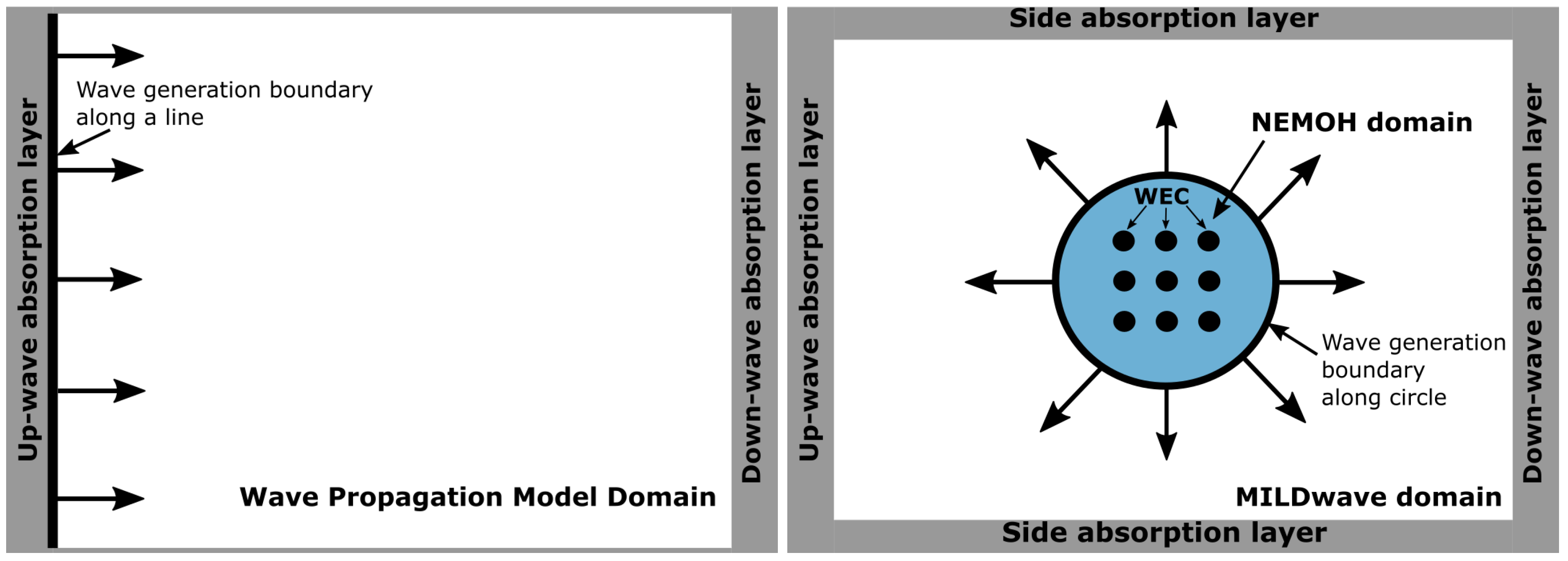
The aforementioned coupling methodology can also be classified into a one-way coupling or two-way coupling depending on how Step 4 is implemented. Figure 3 shows the schematics of a one-way and a two-way coupling, respectively. The inner model domain corresponds to the location of the structure(s), where the near field effects are solved. The outer model domain corresponds to the area where the far field effects are evaluated. Both the inner model domain and the outer model domain are represented not to scale. In a one way-coupling, the wave field for each numerical problem is calculated independently. Thus, the main coupling mechanism in this example is the superposition of two different simulations obtained in the wave propagation model: an incident wave field calculated intrinsically and a perturbed wave field calculated using a wave generation boundary. In a two-way coupling, there is an exchange of information between the wave propagation model and the wave-structure interaction solver in each time step of the simulation and therefore Steps 2, 3 and 4 of the coupling methodology have to be re-calculated at each simulation time step.
Nevertheless, both solutions are able to obtain the far field effects of the WEC array at a reasonable computational cost and accuracy taking into account bathymetric effects and wave transformation processes, with an accurate description of the perturbed wave field around the structure/WEC.
The proposed coupling methodology is a generic tool that can be applied in the following cases:
- Any wave-structure interaction solver that describes the perturbed wave field is suitable for obtaining the input parameters for the internal wave generation boundary. Models based on potential flow theory (e.g., BEM [17,22,23]) or analytical models based on analytical calculation of coefficients or numerical models based on resolving the Navier–Stokes equations (e.g., CFD [6] or SPH) are all suitable in obtaining the perturbed wave field around the WEC array [20].
- Any wave propagation model can be used. A wave propagation boundary can be implemented in both phase-resolving and phase-averaging models.
- The methodology applies to any kind of oscillating or floating structure. In this paper, a WEC array of heaving point absorber WECs is modelled using a phase-resolving model (in order to demonstrate this numerical coupling methodology). However, it can be applied to oscillating water column WECs, overtopping WECs, wave surge WECs, floating breakwaters or platforms.
3. Application of the Coupling Methodology between the Wave Propagation Model, MILDwave, and the BEM Solver, NEMOH
In this section, the generic coupling methodology presented in Section 2 will be demonstrated for obtaining the far field effects due to a WEC array. First, the applied wave theory is discussed. Secondly, a description of the two numerical models employed is provided. Thirdly, the application of the coupling methodology is described for regular and irregular waves. Finally, the coupling methodology is validated against WEC array experimental data from the WECwakes project [1,24,25] which has been co-ordinated by the co-authors of the present paper.
3.1. Numerical Background
3.1.1. Linear Potential Flow
Both models employed are based on linear potential flow theory [22] that allows the flow velocity, , to be expressed as the gradient of the potential, :
The assumptions underlying potential flow theory are the following:
- The flow is inviscid.
- The flow is irrotational.
- The flow is incompressible.
The standard assumption of linear theory that the motion amplitudes of the bodies are much smaller than the wavelength also applies. Linear potential flow theory has hitherto been utilized in a majority of the investigations into WEC array modelling—for example, see [26]. Due to the principle of superposition, linear potential theory allows for the separation of the total wave field into the following components of the velocity potential:
where is the total velocity potential, is the incident wave velocity potential, is the diffracted wave velocity potential and is the sum of the radiated wave velocity potentials for each degree of freedom of motion of the WEC(s). In our investigation, we also make use of the term “perturbed wave” to denote the wave resulting from the sum of the diffracted and radiated wave velocity potentials.
3.1.2. Wave Propagation Model MILDwave
The wave propagation model chosen for demonstrating the coupling methodology is the mild-slope wave propagation model MILDwave [21,27]. MILDwave is a phase-resolving model based on the depth-integrated mild-slope equations of Radder and Dingemans [28]. MILDwave allows for solving the shoaling and refraction of waves propagating above mild-slope varying bathymetries. Furthermore, MILDwave has been widely used in the modelling of WEC arrays [12,16,17,19,24,27,29,30]. The mild-slope equations (Equations (3) and (4)) are resolved using a finite difference scheme that consists of a two-step space-centered, time-staggered computational grid, as detailed in [31]:
where and are, respectively, the free water surface elevation and the wave velocity potential at the free water surface, g is the gravitational acceleration, C is the phase velocity and is the group velocity for a wave with wave number k and angular frequency .
3.1.3. Wave-Structure Interaction Solver NEMOH
The wave-structure interaction solver chosen for demonstrating the coupling methodology and to solve the diffraction/radiation problem is the open-source potential flow BEM solver NEMOH. Given Equation (1), NEMOH solves the Laplace Equation (5) for the complex wave velocity potential, :
given a set of boundary conditions on the wetted body surface, the free surface, sea bottom and the far field area. Equation (5) is solved by employing Green’s functions [15]. An important restriction imposed by Green’s functions is the assumption that the water depth h is constant throughout the BEM domain. The free surface elevation is calculated by taking the real part of the complex potential from the free surface boundary condition, presented by Equation (6). From the superposition principle, presented by Equation (2), free surface elevations can be obtained separately from the vertical motions of the WEC(s) due to the diffracted and radiated potentials:
3.1.4. Modelled WECs
The examined WEC array consists of nine heaving buoys. The buoy shape is a flat circular cylinder with a diameter of 10 m and a draft of 2 m. The shape was chosen to represent several promising WEC technologies that are being developed at the moment [32]. The Power Take-off (PTO) of each WEC is modeled as a resistive damper. The damping coefficient of the PTO, , is kept constant during the investigation with = × kgs. The chosen leads to a resonance condition for a wave period of 8 s [18]. However, it has been found that a variation of depending on the wave period does not have a significant impact on the WEC motion [16]. The WEC array layout is sketched in Figure 4. Here, = 30 m and = 30 m are the inter-array separation distances, = 30 m and = 120 m are the total array dimensions and the WEC array is located at the center of the domain with co-ordinates x = 0 m and y = 0 m. The layout is a staggered grid lay-out. The array layout is kept constant during the analysis.
3.1.5. Wave Characteristics
The results presented here comprise two sets of regular and irregular waves included in Table 1. We aim to demonstrate the application of the coupling methodology and impact of the WEC array on the wave field for different wave periods and for a fixed wave direction = 0. The regular wave set consists of a wave height H = 2 m and a wave period T = 6, 8 and 10 s. The irregular wave set consists of a significant wave height = 2 m and a peak period = 6, 8 and 10 s. The three wave periods chosen range from 6 to 10 s as they range from values closer to the resonance period () of the WECs, for which the WEC motions are large, to values far from where the motions of the WECs are reduced reproducing possible operational wave conditions for the WEC array.
For the regular wave cases (A–C), the results are presented in all points of the domain by calculating the , defined as the ratio between the numerically calculated total wave, , and the incident wave height, :
where is the resulting surface elevation in each simulation time step and is the time window over the is computed.
For the irregular wave cases (D–F), a Pierson–Moskovitz spectrum is utilized to represent a realistic sea state [33]. This methodology for generating irregular waves has already been used by [34] when modelling WEC arrays.
The wave spectrum is discretized in a total of n = 20 regular wave components. The wave height and wave amplitude corresponding to each regular wave component of wave frequency is obtained by:
where = 0.2 corresponds with the wave frequency discretization of the spectrum and with a random number between and corresponds to the phase angle of each wave frequency component.
The surface elevation for each regular wave component is then obtained using Equation (13):
where corresponds to the surface elevation of unit wave amplitude for the ith regular wave component of the wave spectrum.
The irregular surface elevation at each point of the numerical domain is then obtained as a superposition of the N regular wave components of the spectrum using Equation (14):
As in the case of regular waves, the results are presented as the for irregular waves, defined as the ratio between the numerically calculated significant wave height, , and the incident significant wave height, :
3.2. Coupling Methodology Implementation
This section shows the application of the generic coupling methodology using the selected numerical models. The objective is to obtain the total wave field in the MILDwave domain due to the presence of the WEC array. This is performed by superimposing the incident wave field, the diffracted wave field and the radiated wave field generated in MILDwave. The first step (Step 1 in Figure 2) of the coupling methodology is to obtain the incident wave field in the wave propagation model, MILDwave, at the location of the WEC array (Figure 2). A numerical basin is set-up in MILDwave where the incident waves are generated along a linear wave generation boundary perpendicular to the wave propagation direction. In the MILDwave domain, both constant or varying bathymetries can be modelled. To minimize unwanted wave reflection absorption zones (implemented in MILDwave as sponge layers), are placed down-wave and up-wave the basin. From this simulation, the surface elevations at the WEC array location are obtained and used as the input value for NEMOH, which is Step 2 in Figure 2.
In the second step (Step 2 in Figure 2) of the coupling methodology, the radiated/diffracted wave field is obtained around the WEC array using the wave-structure interaction solver NEMOH. NEMOH resolves the wave frequency dependent wave radiation problem for each individual WEC and the diffraction over a predetermined numerical grid. The input values for NEMOH are the WEC array, the wave amplitude at the WEC array location obtained in Step 1, the wave period and the water depth at the WEC array location. As a result, NEMOH gives the complex radiated and diffracted wave fields described by Equations (16) and (17) respectively:
where corresponds to the wave angular frequency (rad/s), i is the imaginary number part, and correspond to the radiated and diffracted wave phase angle, respectively, M is the total number of WECs and is the Response Amplitude Operator (RAO) of each WEC given by:
Here, corresponds to the wave amplitude at the coupling region, is the excitation force, M is the WEC mass, is the added mass, is the hydrodynamic damping coefficient, is the Power Take-Off damping coefficient and is the hydrodynamic stiffness.
The radiated and diffracted wave fields are then summed up in the frequency domain to obtain the perturbed wave field:
In the third step (Step 3 in Figure 2), the perturbed wave field is then transformed from the frequency domain to the time domain and propagated into MILDwave using a circular wave generation boundary (Figure 5). Waves are forced away from the circular wave generation boundary by imposing the free surface elevation along the circle, :
To avoid wave reflection, absorption layers (implemented in MILDwave as sponge layers) are placed up-wave, down-wave and also along the sides of the MILDwave numerical domain. In the fourth step (Step 4 in Figure 2), the incident wave field obtained in Step 1 and the perturbed wave field obtained in Step 3 are combined to obtain the total wave field due to the presence of the WECs array in the MILDwave domain:
3.3. Experimental Data-Set Used for Numerical Validation Purposes
This section gives a description of the experimental data-set used to validate the coupling methodology described in this study. The experimental data-set from the WECwakes project [1,24,25] conducted in the Shallow Water Wave Basin of DHI, Hørsholm, Denmark is used. In the WECwakes project, WEC arrays up to 25 devices were tested to study near field and far field effects of heaving point absorber WECs. First, the characteristics of an individual WEC are described. Secondly, a description of the wave basin is provided. Thirdly, a general description of the WECwakes experiment is included. Finally, the numerical model implementation of the experimental set-up is discussed.
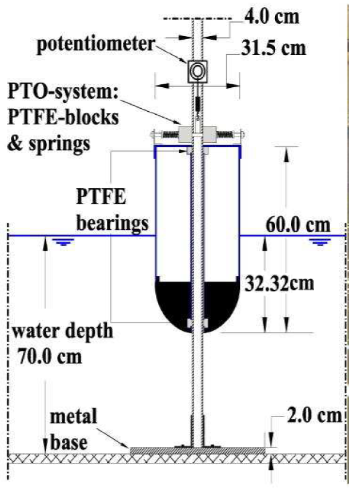
Each of the 25 WEC heaving point absorbers tested consists of a buoy heaving through a metallic vertical shaft mounted on a metal base installed at the bottom of the wave basin (Figure 6). Each buoy consists of a cylindrical body and a spherical bottom with a diameter of 0.315 m. The draft of the WEC is 0.323 m. The water depth is fixed to 0.700 m. The PTO system is composed of Teflon (PTFE)-blocks at the top, which causes energy dissipation through friction damping of the WEC heave motion. Additionally, the presence of the vertical shaft through the buoy causes additional frictional forces on the WEC buoy.
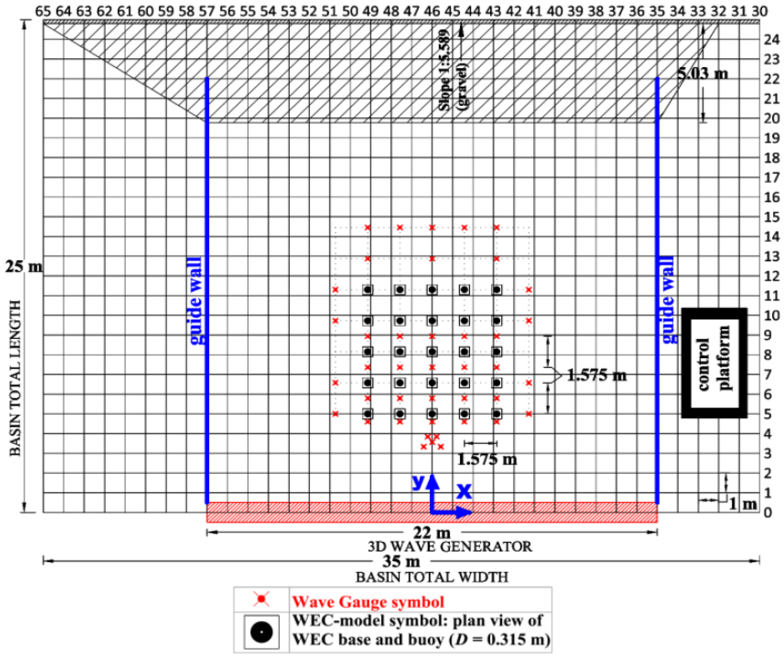
The DHI wave basin experimental domain is 22 m wide and 25 m long and overall depth of 0.8 m. Forty-four piston type wave paddles, each of width 0.5 m generate waves at one end of the wave basin. During the WECwakes project, arrays of up to 25 heaving point absorber WECs (see Figure 7) have been tested using different geometric WEC array configurations. By testing different WEC array configurations under a wide range of sea states a large experimental data-set has been generated and is publicly available for numerical validation purposes. The wave field around the WECs is recorded using 41 resistive wave gauges (WGs) distributed in the basin as shown in Figure 7. A potentiometer is installed at the top of each WEC unit to measure its heave displacement. Furthermore, two load cells were installed in the five WECs located on the central line of the array to measure surge forces.
The WECwakes project has led to a database of 591 test focusing on different array geometrical configurations and wave characteristics. For this validation, an array of nine WECs arranged in a 3 × 3 WEC layout has been selected (see Figure 8). A total of 15 wave gauges located in the front, leeward and sides of the array are identified to compare the free surface elevations between the NEMOH-MILDwave coupled model and the experimental data-set. The separating distance between the different WEC units is equal to 1.575 m. The incident regular wave conditions used are a wave height of H = 0.074 m and a wave period of T = 1.26 s.
The effect of the WEC’s PTO system is included in the numerical simulation by adding an external damping coefficient, , to the equation of motion (Equation (18)). The value for is calculated empirically to account for (i) the PTO system itself which mimics a coulomb damper, (ii) viscous damping of the WEC’s motion due to the presence of water between the vertical supporting axis and the shaft through the WEC unit [35] and (iii) the wave-induced surge forces pushing the WEC against its vertical supporting axis [36]. Therefore, a single WEC has been modelled in NEMOH, similar to the experimental set-up but without the shaft bearing, and regular waves are generated. When the difference between numerical and experimental results of the free surface elevations of the total wave field was smaller than 5%, the applied external damping coefficient is considered sufficient. This methodology resulted in a value of = 28.5 kg/s.
3.4. Test Program
3.4.1. Coupling Methodology Implementation for Constant Bottom Bathymetry
The first objective of this research is to show the accuracy of the NEMOH-MILDwave coupled model in obtaining the total wave field around a WEC array. A comparison between NEMOH and the NEMOH-MILDwave coupled model will be done using the numerical results from NEMOH as a benchmark for the NEMOH-MILDwave coupled model. To quantify the difference in the between NEMOH and the NEMOH-MILDwave coupled model, the relative difference between NEMOH and the NEMOH-MILDwave coupled model is determined:
A test program, Table 2, has been designed based on the regular waves and irregular waves cases presented in Table 1. The total wave field around the 9-WEC array illustrated in Figure 4 is simulated in deep water. The direction of the wave propagation, indicated by in Figure 4, is from left to right. The basin water depth is set to a constant depth of d = 40 m to provide deep water conditions.
Tests 1–3 and tests 7–9 are performed using the BEM code NEMOH. NEMOH has important constraints as noted in [15] but accurately solves array interactions within linear theory. To maximize the accuracy of the results, a numerical basin of 800 m × 800 m is used for each simulation with a grid size of 2 m with an equal spacing in x- and y-directions. It has to be noted that the results from NEMOH are used as the input values for the NEMOH-MILDwave coupled model. NEMOH gives the total wave field individually for each body; however, the 9-WEC array is implemented directly in the NEMOH-MILDwave coupled model.
Tests 4–6 and 10–11 are performed using the NEMOH-MILDwave coupled model. The coupling methodology is implemented along an internal circular wave generation boundary of coupling radius = 120 m. According to [16], a wave generation circle with a minimum rc distance equal to the distance from the center of the coupling region to the most further WEC + 2· offers an accurate solution. The grid size for the simulation is set to 2 m with an equal spacing in the x- and y-directions and an effective domain of 2800 m × 1600 m. Absorbing sponge layers are placed in the edges of the numerical basin to avoid wave reflection. Each simulation is run for 2000 s to obtain a fully developed sea state.
3.4.2. Coupling Methodology Validation for Constant Bottom Bathymetry against Experimental Data
The second objective of this research is to validate the NEMOH-MILDwave numerical model against existing experimental data. For this purpose, the experimental set-up presented in Section 3.3 will be simulated using the coupling methodology presented in Section 3. The 3 × 3 WEC array show in Figure 8 is implemented in the MILDwave domain at a distance of 6.575 m from the wave generation line within an internal circular wave generation boundary of coupling radius = 2.5 m. The wave height is H = 0.074 m and the wave period is T = 1.26 s. The numerical basin depth is set to a constant depth of d = 0.7 m. The grid cell size for the simulation is set to = = 0.04 m with an equal spacing in the x- and y-directions over a MILDwave effective domain of 25 m × 22 m. Each simulation is run for 100 s to obtain a completely developed wave field.
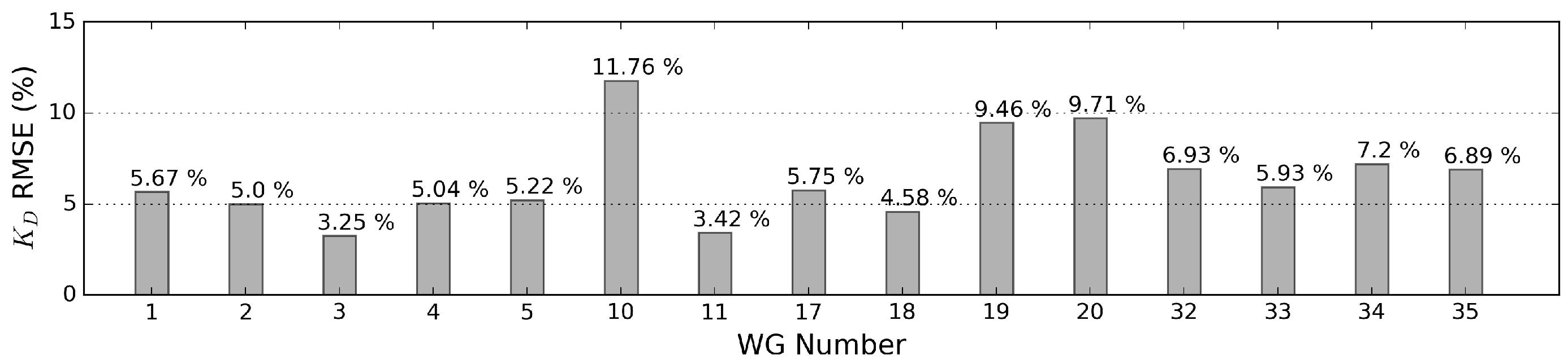
The comparison between the results of the NEMOH-MILDwave model and the experimental WECwakes data is based on the difference of the free surface elevations recorded at the 15 resistive wave gauges (WG) shown in Figure 8. To have a quantitative estimation of the extent of the differences in the free surface elevation, the Root Mean Square Error (RMSE) over a time series of 10 s has been obtained and normalized between the experimental data and the NEMOH-MILDwave coupled model:
3.4.3. Coupling Methodology Implementation for Varying Bathymetry
The third objective of this research is to illustrate the capabilities of the developed NEMOH-MILDwave coupled model to model wave transformations over a large domain. Subsequently, a varying bathymetry (as sketched in Figure 9) is applied to the numerical wave basin by modifying the tests 4–6 and tests 10–12 bathymetrical input (see Table 3). The 9-WEC array (see Figure 4) is placed in the center of the domain at a constant water depth of 20 m. The numerical simulations are performed using identical parameters to those reported in Section 3.1. The latter will provide a benchmark to assess the capability of the model for propagating the wave field over a varying bathymetry.
4. Results
4.1. Coupling Methodology Implementation for Constant Bottom Bathymetry
In this section, the accuracy of the NEMOH-MILDwave coupled model using the presented coupling methodology is discussed. First, the benchmark for the coupling methodology comparison is obtained calculating the total wave field around the 9-WEC array for the BEM model NEMOH. Then, the same simulation is performed using the NEMOH-MILDwave coupled model. Finally, a comparison study between NEMOH and the NEMOH-MILDwave coupled model results is performed by comparing the .
4.1.1. NEMOH Wave Field
The for NEMOH is illustrated in Figure 10. A diffracted-radiated pattern of waves interacting with the WEC array is observed. In front of the WEC array, there is a wave reflection pattern, while, in the lee of the WEC array, there is a wake effect with reduced values of . The diffracted wave pattern does not differ substantially for the three different wave periods both for regular waves and irregular waves. This is due to the fact that the size of the WEC modelled (WEC radius = 5 m) is smaller relative to the incoming wave length. In contrast, the magnitude of the diffracted wave over the radiated wave is increased when the wave period is reduced. As a result, there is almost no wave reflection observed for the case of T = 10 s and = 10 s, while for T= 6 s and 8 s and = 6 s and 8 s the wave reflection pattern is enhanced close to the center of the array, where more WECs are present.
Finally, a comparison between regular and irregular waves shows that less wave reflection occurs in front of the WEC array and reduced wake effect in the lee of the WEC array for smaller wave periods and irregular waves. This decreasing effect possibly originates from the superposition of 20 different frequencies resulting in the total wave field. The superposition of high frequency components will have a major contribution in modifying the incident wave. Due to the type of WEC modelled with a fixed , a larger effect of wave diffraction over wave radiation is observed for higher frequencies. On the contrary, low frequency components will contribute to reduce the wave diffraction and wave radiation effect due to irregular waves as they barely affect the incident wave field. This results in a reduction of both effects when modelling irregular waves leading to smaller values of compared to regular waves.
4.1.2. NEMOH-MILDwave Coupled Model Wave Field
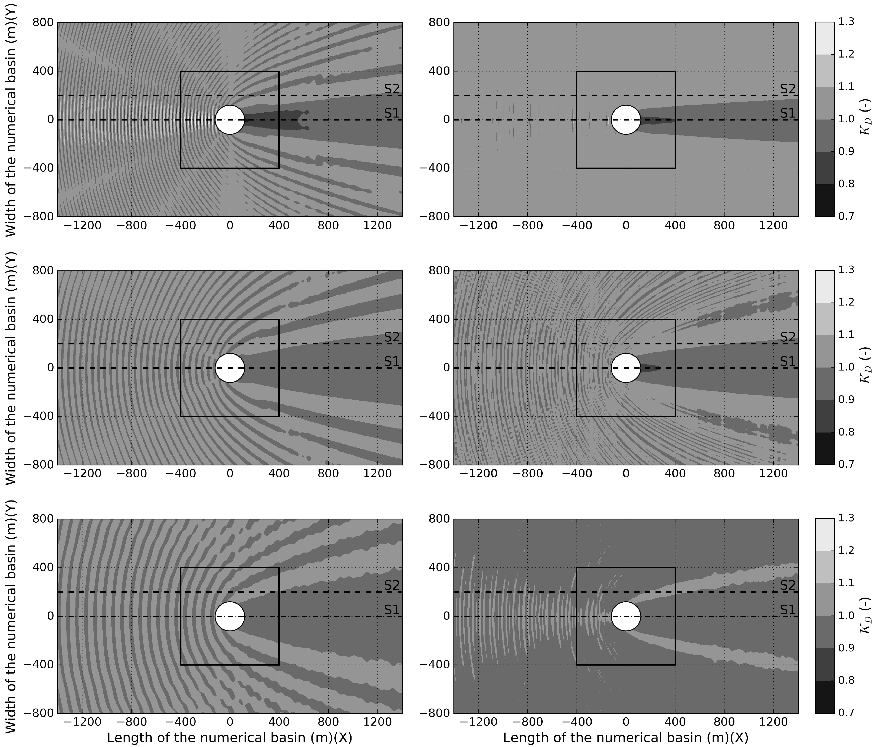
The values for the NEMOH-MILDwave coupled model are illustrated in Figure 11. As reported before, there is a reflection pattern in front of the 9-WEC array while there is a reduction of values in the lee of the WEC array. In contrast to the NEMOH simulations, the numerical domain in MILDwave has now been increased considerably. As a result, it is possible to study the extent of these wave reflection and wake effects in a larger domain overcoming the size limitations of the wave-structure interaction solver. Qualitatively, the wave reflection and wake effects are larger for regular waves than for irregular waves.
4.1.3. Comparison of the Total Wave Field Generated by NEMOH and the NEMOH-MILDwave Coupled Model
The for NEMOH and the NEMOH-MILDwave coupled modes results are depicted in Figure 10 and Figure 11, respectively. The observed close to the internal coupling generation line is slightly different in Figure 10 and Figure 11. In front of the WEC array, there is a positive difference in of 0.02 between NEMOH and the NEMOH-MILDwave coupled model, while, in the lee of the array, there is a negative difference in of −0.01. Despite these small differences, on a region of 800 m × 800 m around the 9-WEC array, the obtained correspondence of the results is very good.
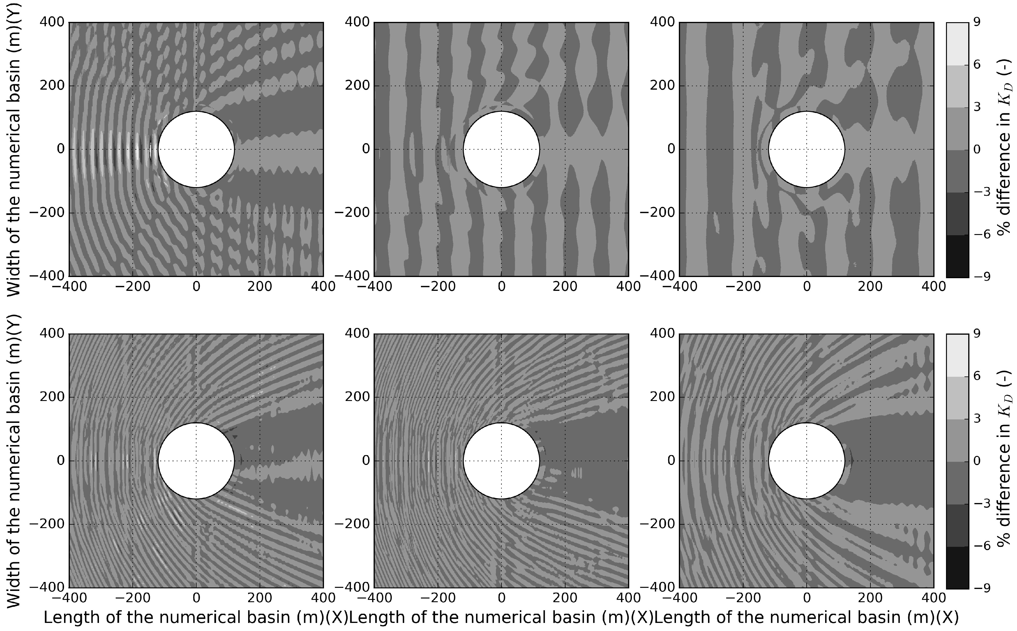
In Figure 12, six plots show the relative % difference in between the two models for the wave periods studied for regular and irregular waves. The coupling region is masked out in a white circle as the total wave field in this region corresponds to the NEMOH results.
The largest observed relative % difference in between the NEMOH-MILDwave coupled model and the NEMOH model is located in the region in front of the array for all cases. These relative % differences in never exceed 7% for all cases. Moreover, the difference in the observed total wave field is higher for regular waves than for irregular waves, being maximized for smaller periods. Thereafter, there is an overestimation in the NEMOH-MILDwave model when propagating the internal prescribed perturbed wave. This overestimation is concentrated locally close to the coupling region up to a maximum value of 3% and is reduced when moving away from it. Subsequently, an assumption can be made that the NEMOH-MILDwave coupled model is accurate when propagating the wave field on a large domain.
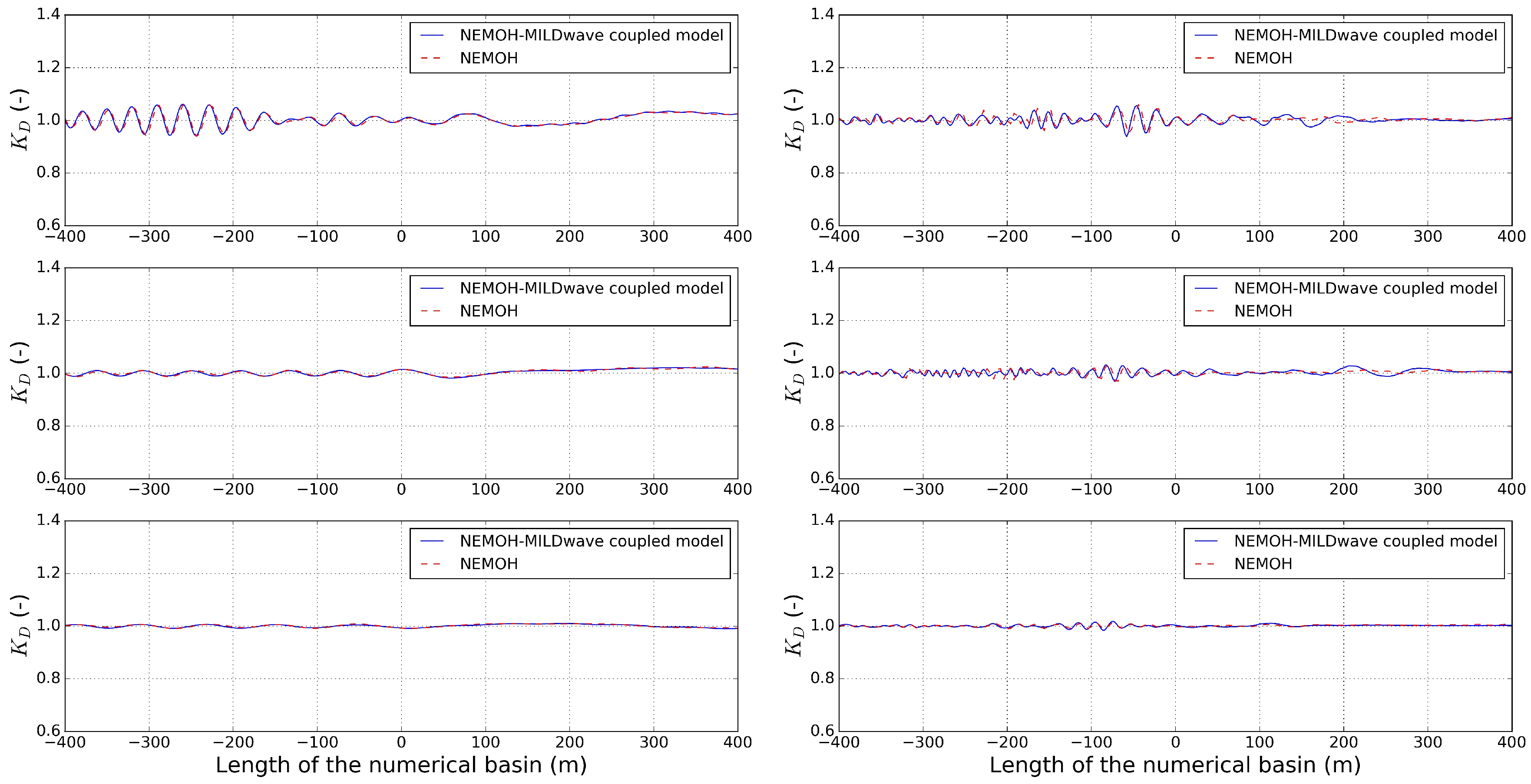
To have a better look at the agreement between the NEMOH-MILDwave coupled model and NEMOH, longitudinal cross-sections are taken at two different locations: S1 at the center of the domain, y = 0 m (Figure 13), and S2 with an off-set of 200 m along the y-axis, y = 200 m (Figure 14). The cross-sections shown on the left side of the figures correspond to regular waves, while the cross sections shown on the right side of the figures correspond to irregular waves. The near field region that is modelled with NEMOH and is not part of the coupling methodology analysis is masked out in gray between two black vertical lines. Both coupled models show a good correlation as the values of obtained are close to each other. As it has already been mentioned, for irregular waves, the wake behind the WEC array is increased in both magnitude and distance but is narrower, in contrast to the higher wave reflection values in front of the WEC array given for regular waves.
4.2. Coupling Methodology Validation for Constant Bottom Bathymetry against Experimental Data
The comparison between the NEMOH-MILDwave coupled model and the experimental data is shown in Figure 15. Overall, there is a good agreement between the NEMOH-MILDwave coupled model and the experimental data as it can be seen in Figure 15. However, it can be noticed that wave gauges 1, 10, 20, 32 and 33 show small differences on the surface elevation pattern.
The error of the free surface elevation for each wave gauge is included in Figure 16. It can be seen that the best agreement is obtained in front of the WEC array (WG 1-5) and in the wake of the array (WG 11) with an error ranging from 3–5%. The biggest difference is also obtained in the wake of the array (WG10) close to the WEC array with an error of 11%. While evaluating this biggest difference, it has to be considered that experimental data is intrinsically nonlinear [24]. Nonlinear effects such as viscosity or the friction between the shaft an the WECs cannot be modeled with the coupling methodology employed as it is based on linear wave theory. This cannot be modeled with the coupling methodology employed as it is based on linear wave theory. When the wave propagates further from the WEC, these nonlinearities are reduced and therefore the agreement between experimental and numerical data is better. Finally, on the sides of the coupling region the error ranges from 6 to 9% showing that the numerical model is not accurately representing the wave diffraction around the WEC array.
It has to be noted, however, that, within this numerical validation, a linear model is compared with experimental data that has nonlinear effects. Therefore, it can be seen that further away from the location of the WEC array, a better agreement in the free surface elevation is obtained.
4.3. Coupling Implementation for Varying Bathymetry
The are given in Figure 17 for both regular and irregular waves. Again, a wave reflection pattern is formed in front of the WEC array and a reduction in values appears in the lee of the WEC array. However, the presence of the bathymetry is changing the magnitude of the wave radiation and wave diffraction effects. As mentioned in Section 4.2, there is a reduction in the extent of the wake effects for higher periods and for irregular waves. In contrast to the constant bathymetry case, the extension of the wake effect tends to disappear with an increasing wave period for a varying bathymetry. Furthermore, there is a reduction in the wave reflection pattern up-wave. This is due to the shoaling effect that is expected to be bigger on waves with a larger wave length and consequently has a higher impact in higher wave periods than the generated wake behind the WEC array which is lower. Only for T = 6 s does the array total wave field modification outweigh the shoaling effects and thus the WEC array has an impact both up-wave and down-wave. For the other two wave periods modelled, the effect of the WEC array is practically nil in the region down-wave the WEC array where the shoaling effects are much greater than the wake effects.
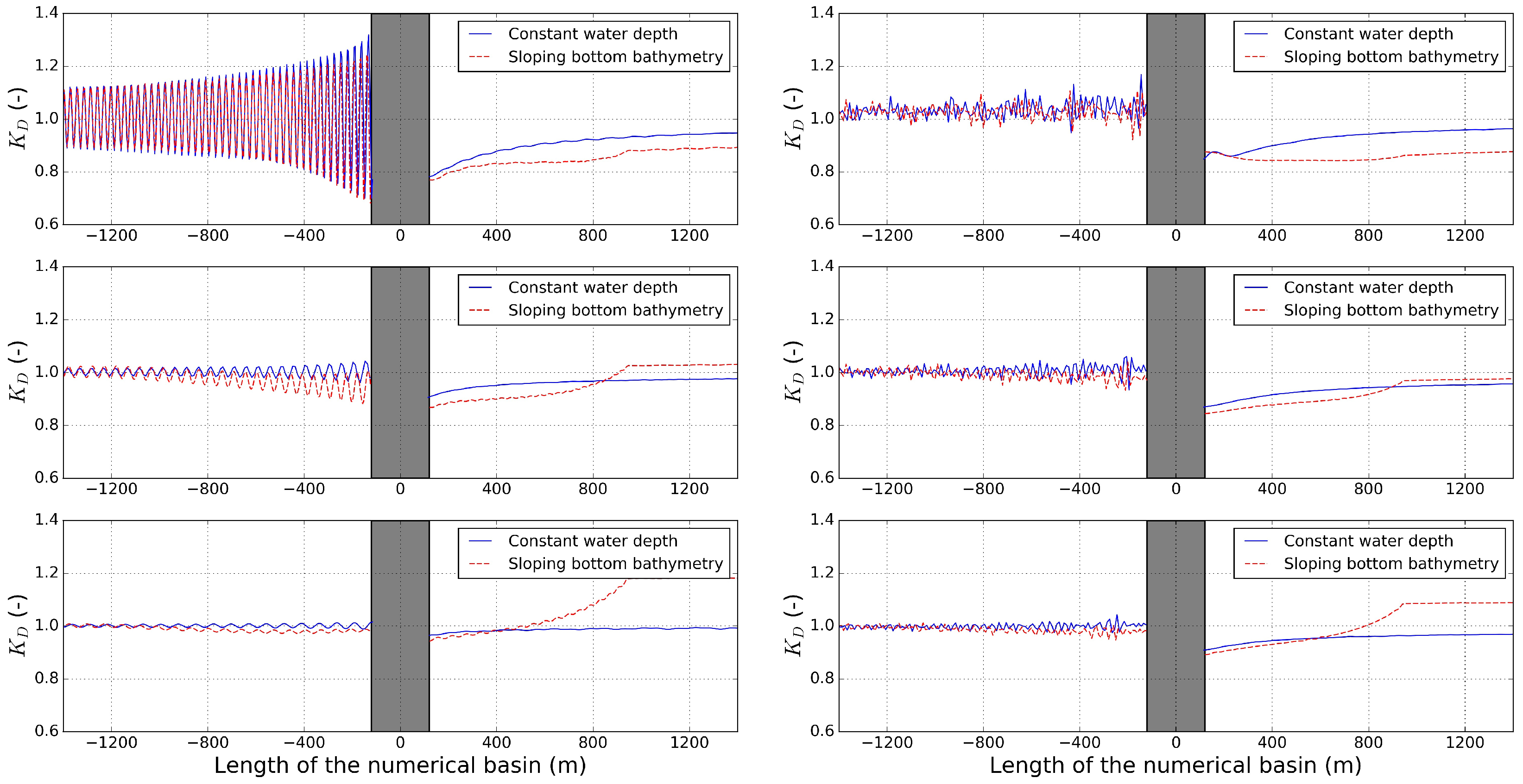
To have a closer look at the effects of shoaling over the wave field generated around the WEC array, a longitudinal cross-section S1 is taken at the center of the domain, y = 0 m (Figure 18), for the constant and irregular bathymetry test cases. The cross-sections shown on the left side of the figures correspond to regular waves, while the cross sections shown on the right side of the figures correspond to irregular waves. The coupling region is masked out in gray between two vertical black lines, as the results between NEMOH and the NEMOH-MILDwave coupled model cannot be compared. Consistently, the influence of shoaling over wave reflection and wave diffraction effect of the WEC array is reduced with a reduction in the wave period. It can be observed that the changes in the wave reflection magnitude are due to the reduction of the incident wave caused by bottom induced propagation effects in the wave propagation model MILDwave. On the contrary, the reduction of the extent of the wake effects is generated by the increase of the wave height as the shoaling effect takes over.
5. Discussion
In Section 4.1, it can be seen that the NEMOH-MILDwave coupled model can accurately propagate the total wave field around a WEC array according to linear wave theory. Nevertheless, there are some discrepancies for between NEMOH and the NEMOH-MILDwave coupled model close to the coupling region. These relative differences for remain under 3%. Moreover, when moving away from the coupling region these relative differences in are reduced. These reductions in the error are showing that the complexity of the hydrodynamic interactions when modelling the far field effects is not that influential, as wave diffraction and wave radiation effects diminish with distance. As a result, it can be concluded that the NEMOH-MILDwave coupled model is able to replicate the numerical NEMOH simulation and extend it to a larger domain. Furthermore, the simulations in Section 4.1 have been extended including a varying bathymetry in Section 4.3. Those simulations have given good results, showing the effect of bottom induced propagation effects over the wave reflection and wake effects caused by the WEC array in the incident wave. Subsequently, it has been demonstrated that the NEMOH-MILDwave coupled model can be used to analyze the impacts of a WEC array in a wave field over a varying bathymetry over a large coastal zone.
However, coupling NEMOH and MILDwave has some limitations. Firstly, despite the fact that the time spent to compute a small WEC array in this study is not very long, it can increase considerably when increasing the number of WECs present. The NEMOH simulations are performed for nine WECs with one degree of freedom (DOF) and one direction. For an array of J WECs with six DOFs, the computational time of a BEM model increases as , with increased simulation time in larger domains. Consequently, the maximum number of WECs that can be used is limited. Secondly, NEMOH calculations can only be performed on a constant bathymetry. This assumption is valid for closely spaced WECs in deep water. However, when the WECs are placed in intermediate or shallow waters, the effects of the bathymetry are significant as shown in Section 4.2 and according to [18]. It is necessary to study the influence of the bathymetry in closely space WEC arrays in order to define the extent of the WEC array that can be modelled. Thirdly, irregular waves are calculated as a superposition of regular waves. To increase the accuracy of the results, an increase in the number of regular wave components is required, resulting in more computational time. Finally, a heaving buoy modelled with a passive resistive PTO has an effect on the surrounding areas that is highly influenced by wave diffraction and not so much by wave radiation. This clearly shows the importance of the frequency distribution in the WEC array effects and the need for a realistic modelling of the WEC PTO to maximize the power output and thus quantify its effect on the surrounding wave field [37].
In terms of limitations of the proposed coupling methodology, these depend each time on the type of models that are coupled. Specifically for coupling between two linear models such as NEMOH and MILDwave which are used here, the resulting coupled model will provide conservative results in study cases when nonlinear phenomena are dominating. Moreover, MILDwave is applied for mild-slope bathymetries. On the other hand, the above limitations can be overcome when applying the proposed coupling methodology, if, for instance, nonlinear models are coupled (which however often introduce computational instability and high computational cost).
6. Conclusions
In this paper, a generic coupling methodology has been presented to calculate far field effects of floating structures. The wave propagation model MILDwave and the wave structure interaction solver NEMOH are combined to model the wave field propagating around a WEC array under regular and irregular waves over a constant or varying bathymetry. Pairing models with different resolutions enables the modeler to obtain accurate results within a reasonable computational time. It has been demonstrated that there is a good agreement between the NEMOH-MILDwave coupled model and the NEMOH solution in the close proximity of the coupling region for both regular and irregular waves. As a result, it can be assumed that the NEMOH-MILDwave coupled model can be extended to larger domains. Furthermore, a good agreement is obtained between numerical and experimental results. Even though there are some discrepancies between the numerical and experimental results, these discrepancies are mainly caused due to non-linear effects during the experiments. The numerical results have been extended to a varying bathymetry. It is seen that the bathymetry highly influences the total wave field around the WEC array and thus the coupling methodology presented provides itself as a useful numerical tool for wave energy studies assessing the coastal impact of WECs arrays within linear wave theory. The numerical results have also shown some limitations regarding computational time, the number of WECs modelled and the accuracy of PTO modelling. Regardless of this limitations, the NEMOH-MILDwave coupled model introduced has proven to be a reliable tool that can be applied in a fast and efficient way to calculate far field effects of WEC arrays. The next steps in our modelling work is to extend the methodology to real bathymetries in the MILDwave domain to study the effect of WEC arrays on a real case scenario. As MILDwave correctly models coastal transformation processes, this will allow for calculating the impact of a wave farm on any particular coastal area given any type of WEC. Different array and PTO configurations will be tested in order to accurately represent the wave absorption of commercially viable WECs.
Author Contributions
G.V.F. set up the numerical experiments in collaboration with P.B.; G.V.F. performed the numerical experiments; G.V.F. compared the numerical experiments with experimental data with the assistance of P.B.; V.S. and P.T. have offered the WECwakes project experimental data-set; V.S. and P.T. provided the fundamentals of the coupling methodology; V.S. and P.T. proofread the text and helped in structuring the publication.
Funding
This research received no external funding.
Conflicts of Interest
The authors declare no conflict of interest.
Abbreviations
The following abbreviations are used in this manuscript:
| WEC | Wave Energy Converter |
| BEM | Boundary Element Method |
| CFD | Computer Fluid Dynamics |
| SPH | Smoothed Particle Hydrodynamics |
| PTO | Power Take-Off |
| RAO | Response Amplitude Operator |
| DHI | Danish Hydraulic Institute |
| WG | Wave Gauge |
| RMSE | Root-Mean-Square-Error |
References
- Stratigaki, V. Experimental Study and Numerical Modelling of Intra-Array Interactions and Extra-Array Effects of Wave Energy Converter Arrays. Ph.D. Thesis, Ghent University, Gent, Belgium, 2014. [Google Scholar]
- Child, B.M.F.; Venugopal, V. Optimal Configurations of wave energy devices. Ocean Eng. 2010, 37, 1402–1417. [Google Scholar] [CrossRef]
- Garcia-Rosa, P.B.; Bacelli, G.; Ringwood, J. Control-Informed Optimal Array Layout for Wave Farms. IEEE Trans. Sustain. Energy 2015, 6, 575–582. [Google Scholar] [CrossRef] [Green Version]
- Babarit, A. On the park effect in arrays of oscillating wave energy converters. Renew. Energy 2013, 58, 68–78. [Google Scholar] [CrossRef]
- Borgarino, B.; Babarit, A.; Ferrant, P. Impact of wave interaction effects on energy absorbtion in large arrays of Wave Energy Converters. Ocean Eng. 2012, 41, 79–88. [Google Scholar] [CrossRef]
- Devolder, B.; Rauwoens, P.; Troch, P. Towards the numerical simulation of 5 Floating Point Absorber Wave Energy Converters installed in a line array using OpenFOAM. In Proceedings of the 12th European Wave and Tidal Energy Conference (EWTEC 2017), Cork, Ireland, 27 August–1 September 2017; pp. 739–749. [Google Scholar]
- Abanades, J.; Greaves, D.; Iglesias, G. Wave farm impact on the beach profile: A case study. Coast. Eng. 2014, 86, 36–44. [Google Scholar] [CrossRef]
- Iglesias, G.; Carballo, R. Wave farm impact: The role of farm-to-coast distance. Renew. Energy 2014, 69, 375–385. [Google Scholar] [CrossRef]
- Millar, D.L.; Smith, H.C.M.; Reeve, D.E. Modelling analysis of the sensitivity of shoreline change to a wave farm. Ocean Eng. 2007, 34, 884–901. [Google Scholar] [CrossRef]
- Venugopal, V.; Smith, G. Wave Climate Investigation for an Array of Wave Power Devices. In Proceedings of the 7th European Wave and Tidal Energy Conference, Porto, Portugal, 11–13 September 2007; p. 10. [Google Scholar]
- Smith, H.C.M.; Millar, D.L.; Reeve, D.E. Generalisation of wave farm impact assessment on inshore wave climate. In Proceedings of the 7th European Wave and Tidal Energy Conference, Porto, Portugal, 11–13 September 2007. [Google Scholar]
- Beels, C.; Troch, P.; De Backer, G.; Vantorre, M.; De Rouck, J. Numerical implementation and sensitivity analysis of a wave energy converter in a time-dependent mild-slope equation model. Coast. Eng. 2010, 57, 471–492. [Google Scholar] [CrossRef]
- Folley, M.; Babarit, A.; Child, B.; Forehand, D.; O’Boyle, L.; Silverthorne, K.; Spinneken, J.; Stratigaki, V.; Troch, P. A Review of Numerical Modelling of Wave Energy Converter Arrays. In Proceedings of the ASME 2012 31st International Conference on Ocean, Offshore and Arctic Engineering (OMAE), Rio de Janeiro, Brazil, 1–6 July 2012. [Google Scholar]
- Lee, C.H.; Newman, J.N. WAMIT User Manual, Versions 6.4, 6.4 PC, 6.3, 6.3S-PC; WAMIT, Inc.: Chestnut Hill, MA, USA, 2006. [Google Scholar]
- Babarit, A.; Delhommeau, G. Theoretical and numerical aspects of the open source BEM solver NEMOH. In Proceedings of the 11th European Wave and Tidal Energy Conference, Nantes, France, 6–11 September 2015. [Google Scholar]
- Balitsky, P.; Verao Fernandez, G.; Stratigaki, V.; Troch, P. Coupling methodology for modelling the near-field and far-field effects of a Wave Energy Converter. In Proceedings of the ASME 36th International Conference on Ocean, Offshore and Arctic Engineering (OMAE2017), Trondheim, Norway, 25–30 June 2017. [Google Scholar]
- Verbrugghe, T.; Stratigaki, V.; Troch, P.; Rabussier, R.; Kortenhaus, A. A comparison study of a generic coupling methodology for modeling wake effects of wave energy converter arrays. Energies 2017, 10, 1697. [Google Scholar] [CrossRef]
- Charrayre, F.; Peyrard, C.; Benoit, M.; Babarit, A. A Coupled Methodology for Wave-Body Interactions at the Scale of a Farm of Wave Energy Converters Including Irregular Bathymetry. In Proceedings of the ASME 2014 33rd International Conference on Ocean, Offshore and Arctic Engineering, San Francisco, CA, USA, 8–13 June 2014. [Google Scholar]
- Tomey-Bozo, N.; Murphy, J.; Lewis, T.; Troch, P.; Thomas, G. Flap type wave energy converter modelling into a time-dependent mild-slope equation model. In Proceedings of the 2nd International Conference on Offshore Renewable Energies, Lisbon, Portugal, 24–26 October 2016; pp. 277–284. [Google Scholar]
- Verbrugghe, T.; Devolder, B.; Dominguez, J.; Kortenhaus, A.; Troch, P. Feasibility study of applying SPH in a coupled simulation tool for wave energy converter arrays. In Proceedings of the 12th European Wave and Tidal Energy Conference (EWTEC 2017), Cork, Ireland, 27 August–1 September 2017; pp. 679–689. [Google Scholar]
- Troch, P. MILDwave—A Numerical Model for Propagation and Transformation of Linear Water Waves; Technical Report; Department of Civil Engineering, Ghent University: Ghent, Belgium, 1998. [Google Scholar]
- Alves, M. Wave Energy Converter modelling techniques based on linear hydrodynamic theory. Numer. Model. Wave Energy Convert. 2016, 1, 11–65. [Google Scholar]
- Verbrugghe, T.; Troch, P.; Kortenhaus, A.; Stratigaki, V.; Engsig-Karup, A.P. Development of a numerical modelling tool for combined near field and far field wave transformations using a coupling of potential flow solvers. In Proceedings of the 2nd International Conference on Renewable Energies Offshore, Lisbon, Portugal, 24–26 October 2016. [Google Scholar]
- Stratigaki, V.; Troch, P.; Stallard, T.; Forehand, D.; Kofoed, J.P.; Folley, M.; Benoit, M.; Babarit, A.; Kirkegaard, J. Wave Basin Experiments with Large Wave Energy Converter Arrays to Study Interactions between the Converters and Effects on Other Users. Energies 2014, 7, 701–734. [Google Scholar] [CrossRef] [Green Version]
- Stratigaki, V.; Troch, P.; Stallard, T.; Forehand, D.; Folley, M.; Kofoed, J.P.; Benoit, M.; Babarit, A.; Vantorre, M.; Kirkegaard, J. Sea-state modification and heaving float interaction factors from physical modelling of arrays of wave energy converters. J. Renew. Sustain. Energy 2015, 7, 061705. [Google Scholar] [CrossRef]
- Penalba, M.; Touzón, I.; Lopez-Mendia, J.; Nava, V. A numerical study on the hydrodynamic impact of device slenderness and array size in wave energy farms in realistic wave climates. Ocean Eng. 2017, 142, 224–232. [Google Scholar] [CrossRef]
- Troch, P.; Stratigaki, V. Phase-Resolving Wave Propagation Array Models. Numer. Model. Wave Energy Convert. 2016, 10, 191–216. [Google Scholar]
- Radder, A.C.; Dingemans, M.W. Canonical equations for almost periodic, weakly nonlinear gravity waves. Wave Motion 1985, 7, 473–485. [Google Scholar] [CrossRef]
- Beels, C.; Troch, P.; Kofoed, J.P.; Frigaard, P.; Kringelum, J.V.; Kromann, P.C.; Donovan, M.H.; De Rouck, J.; De Backer, G. A methodology for production and cost assessment of a farm of wave energy converters. Renew. Energy 2011, 36, 3402–3416. [Google Scholar] [CrossRef]
- Stratigaki, V.; Troch, P.; Baelus, L.; Keppens, Y.U. Introducing wave generation by wind in a mild-slope wave propagation model MILDwave, to investigate the wake effects in the lee of a farm of wave energy converters. In Proceedings of the ASME 2011 30th International Conference on Ocean, Offshore and Arctic Engineering, Rotterdam, The Netherlands, 19–24 June 2011. [Google Scholar]
- Brorsen, M.; Helm-Petersen, J. On the Reflection of Short-Crested Waves in Numerical Models. In Proceedings of the 26th International Conference on Coastal Engineering, Copenhagen, Denmark, 22–26 June 1998; pp. 394–407. [Google Scholar]
- National Renewable Energy Laboratory. Marine and Hydrokinetic Technology Database. Available online: https://openei.org/wiki/Marine_and_Hydrokinetic_Technology_Database_759 (accessed on 1 June 2018).
- Faltinsen, O.M. Sea Loads on Ships and Offshore Structures; Cambridge University Press: Cambridge, UK, 1990; p. 328. [Google Scholar]
- Sismani, G.; Babarit, A.; Loukogeorgaki, E. Impact of Fixed Bottom Offshore Wind Farms on the Surrounding Wave Field. Int. J. Offshore Polar Eng. 2017, 27, 357–365. [Google Scholar] [CrossRef]
- Devolder, B.; Rauwoens, P.; Troch, P. Numerical simulation of a single floating point absorber wave energy converter using OpenFOAM. In Proceedings of the 2nd International Conference on Renewable energies Offshore, Lisbon, Portugal, 24–26 October 2016; pp. 197–205. [Google Scholar]
- Devolder, B.; Stratigaki, V.; Troch, P.; Rauwoens, P. CFD simulations of floating point absorber wave energy converter arrays subjected to regular waves. Energies 2018, 11, 641. [Google Scholar] [CrossRef]
- Child, B.M.F. On the Configuration of Arrays of Floating Wave Energy Converters. Ph.D. Thesis, The University of Edinburgh, Edinburgh, UK, 2011. [Google Scholar]
Figure 1.
Visual representation of the near field effects between neighboring oscillating WECs (represented by solid circles) in a WEC array under incident waves [1].
Figure 1.
Visual representation of the near field effects between neighboring oscillating WECs (represented by solid circles) in a WEC array under incident waves [1].

Figure 2.
Flow chart of the generic coupling methodology between a wave-structure interaction solver and a wave propagation model.
Figure 2.
Flow chart of the generic coupling methodology between a wave-structure interaction solver and a wave propagation model.
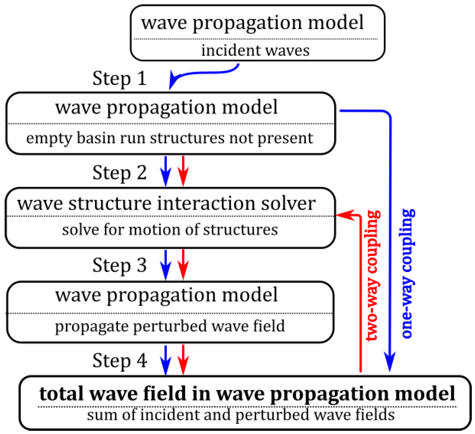
Figure 3.
Schematic of a one-way coupling (left) and two-way coupling (right). In the inner model domain, the motions of the studied structure(s)/WEC(s) are solved.
Figure 3.
Schematic of a one-way coupling (left) and two-way coupling (right). In the inner model domain, the motions of the studied structure(s)/WEC(s) are solved.
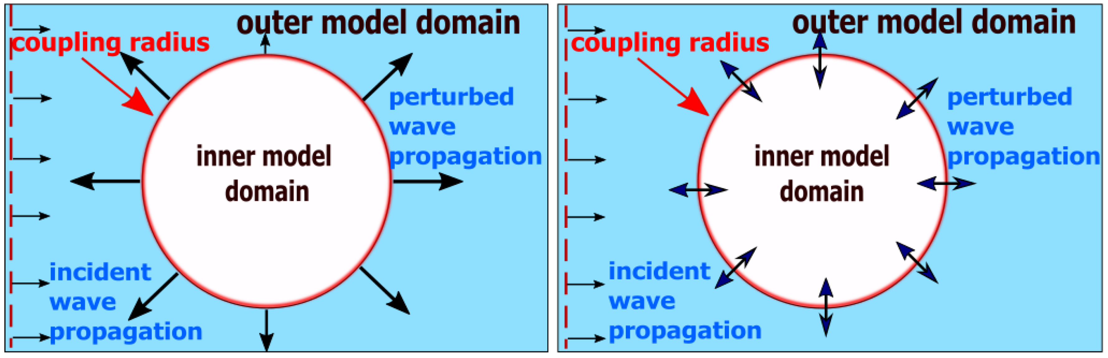
Figure 4.
Plane (Top) view of the WEC array layout for nine heaving buoys. indicates the direction of wave propagation.
Figure 4.
Plane (Top) view of the WEC array layout for nine heaving buoys. indicates the direction of wave propagation.
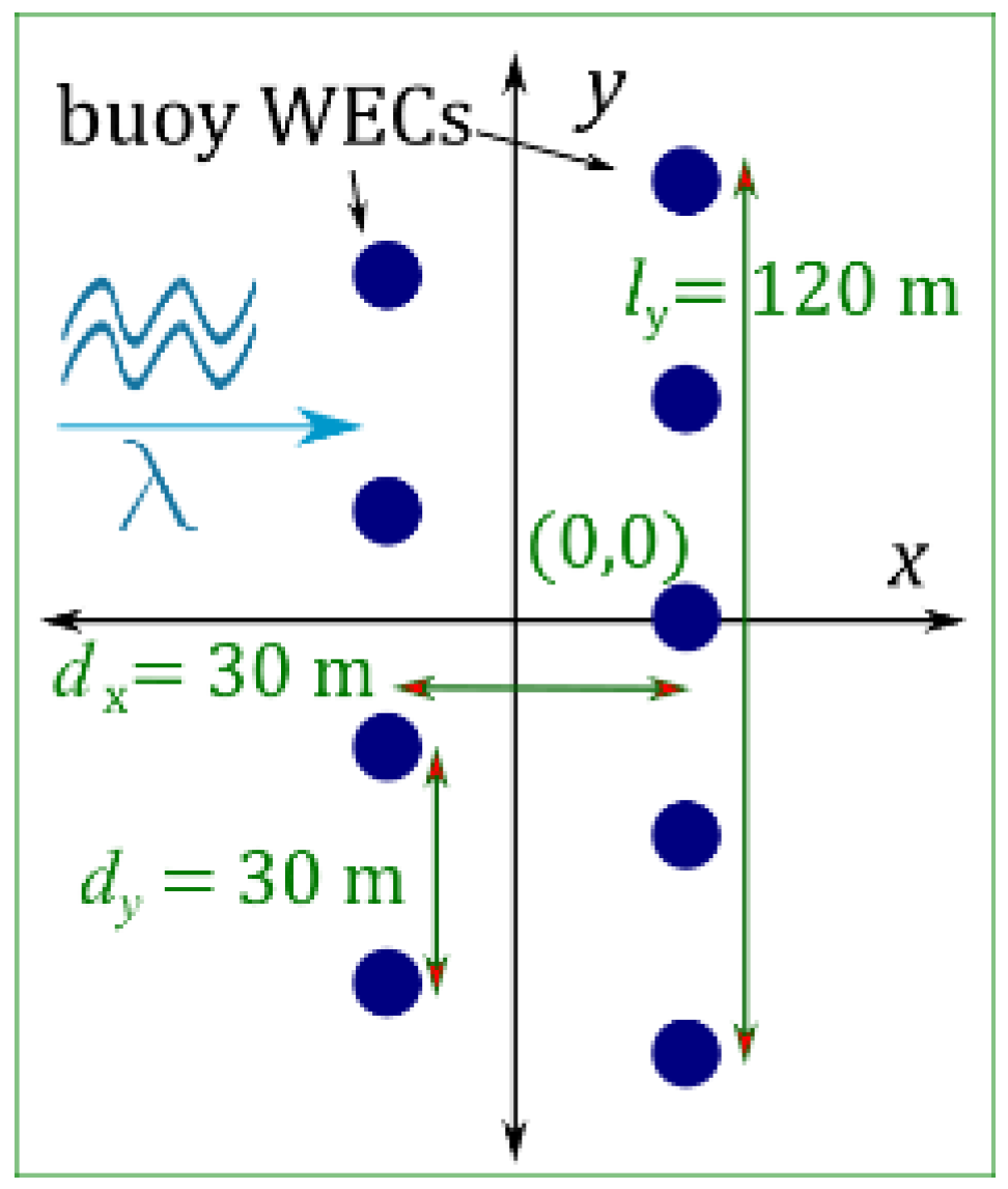
Figure 5.
Sketch of the incident wave propagation (left) and perturbed wave propagation (right) in MILDwave. The black line corresponds to the wave generation line, the black circle corresponds to the circular wave generation boundary and the grey areas correspond to absorption zones (sponge layers) down-wave, up-wave and along the sides of the numerical domain.


Figure 7.
Plan view of the WECwakes experimental set-up in the DHI wave basin as a 5 × 5 rectilinear array. The red crosses indicate the position of all the wave gauges installed in the DHI wave basin during the experiments and the black circles indicate the location of the different WEC units. The wave paddles are denoted by the red hatched area at the bottom of the figure while the black hatched area at the top of the figure represents the installed absorbing beach. Two guiding walls were installed at the sides of the basin, denoted in blue lines [1].

Figure 8.
Set up of the WEC array layout used for the comparison between the coupled model and the experimental tests. WECs are represented by • and wave gauges (WGs) by x. The WG are numbered as they appear in the WECwakes experimental data set. The direction of wave propagation, indicated by , is from left to right.
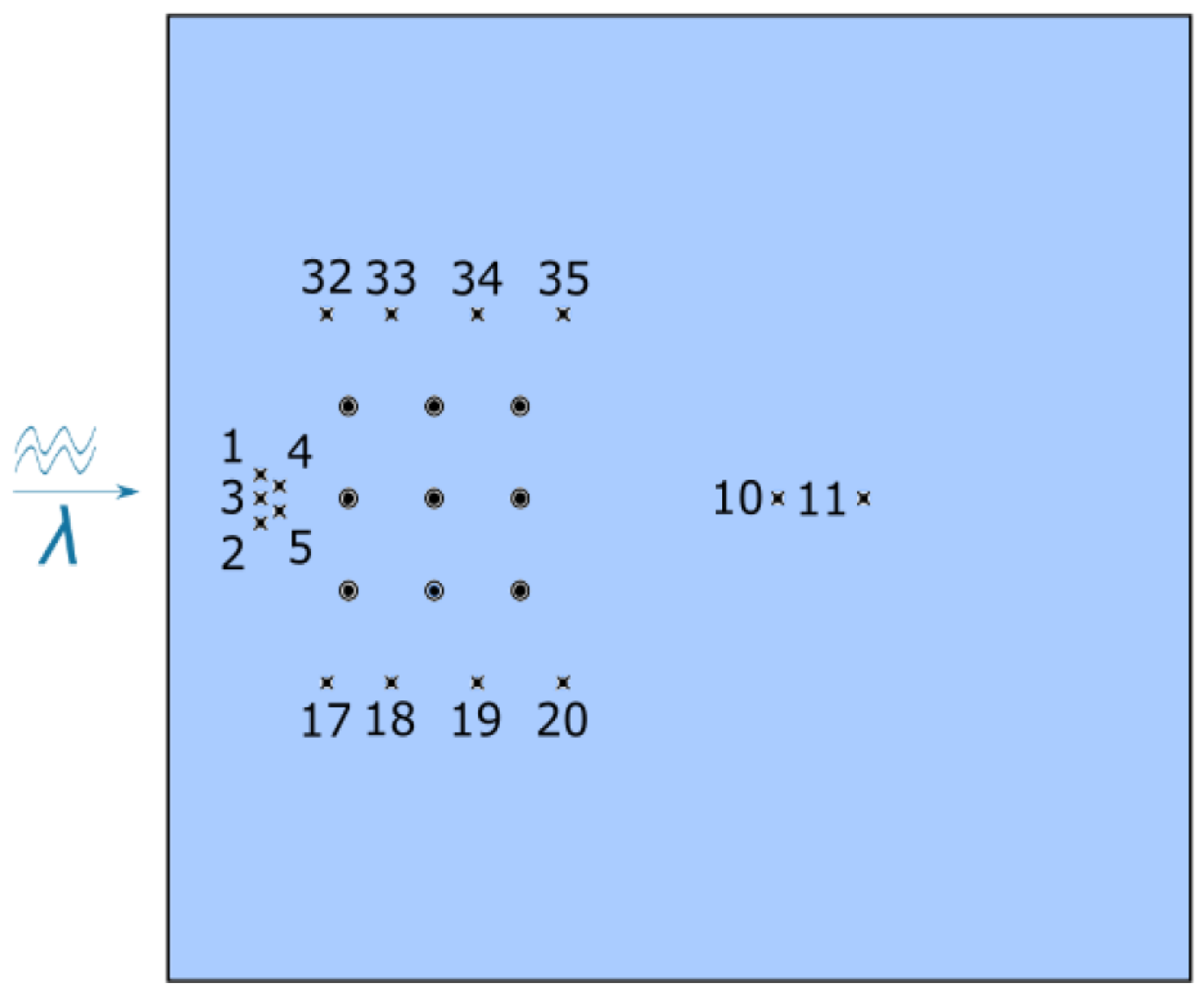
Figure 9.
Depth view showing the location of the 9-WEC array. x–z plane (side) profile. The coastline is located at the right side of the figure. The 9-WEC array is located at the center of the domain.
Figure 9.
Depth view showing the location of the 9-WEC array. x–z plane (side) profile. The coastline is located at the right side of the figure. The 9-WEC array is located at the center of the domain.
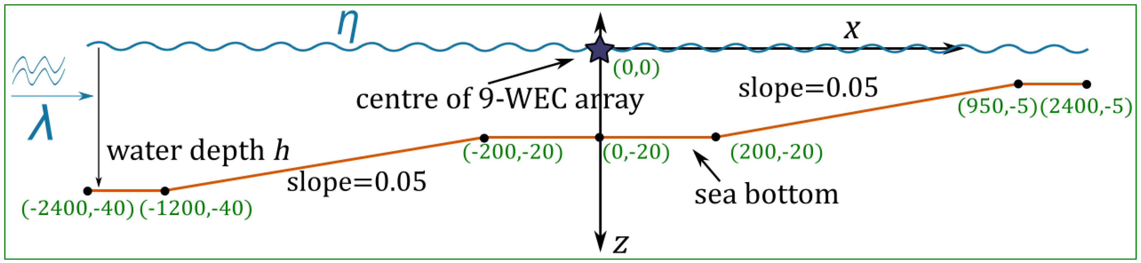
Figure 10.
NEMOH results of for a 9-WEC array for regular waves (top) with T = 6 s (left), T = 8 s (middle) and T = 10 s (right) and for irregular waves (bottom) with = 6 s (left), = 8 s (middle) and = 10 s (right). Contour levels are set at an interval 0.04 m. The white solid circles indicate the location of the WECs
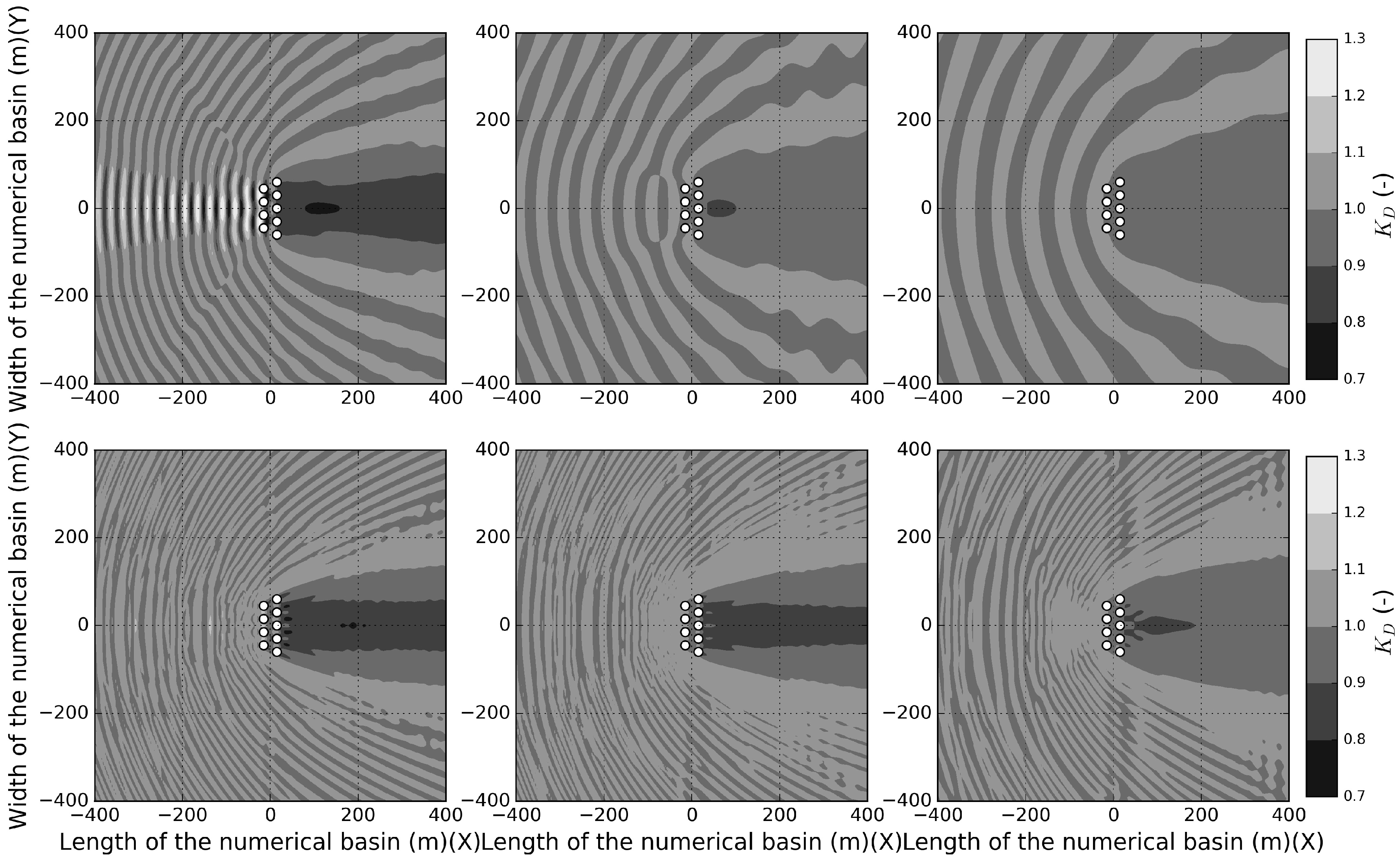
Figure 11.
NEMOH-MILDwave couple model values of a 9-WEC array for regular waves with T = 6 s, T = 8 s and T = 10 s and for irregular waves with = 6 s, = 8 s and = 10 s. Contour levels are set at an interval 0.04 m. The water depth is 40 m. Waves are propagating from left to right. The coupling region is masked out using a white circle and includes the WECs. The NEMOH numerical domain is limited by black square.

Figure 12.
Relative difference (%) in between NEMOH-MILDwave coupled model and NEMOH. Regular waves (top) and Irregular waves (bottom). For regular waves with T = 6 s, T = 8 s and T = 10 s and for irregular waves with = 6 s, = 8 s and = 10 s. The coupling region is masked out using a white circle.
Figure 12.
Relative difference (%) in between NEMOH-MILDwave coupled model and NEMOH. Regular waves (top) and Irregular waves (bottom). For regular waves with T = 6 s, T = 8 s and T = 10 s and for irregular waves with = 6 s, = 8 s and = 10 s. The coupling region is masked out using a white circle.

Figure 13.
Cross-section S1 of the for a 9-WEC array at y = 0 m for regular waves (left) and irregular waves (right) for regular waves with T = 6 s, T = 8 s and T = 10 s and for irregular waves with = 6 s, = 8 s and = 10 s. The coupling region is masked out in gray between two vertical black lines.
Figure 13.
Cross-section S1 of the for a 9-WEC array at y = 0 m for regular waves (left) and irregular waves (right) for regular waves with T = 6 s, T = 8 s and T = 10 s and for irregular waves with = 6 s, = 8 s and = 10 s. The coupling region is masked out in gray between two vertical black lines.
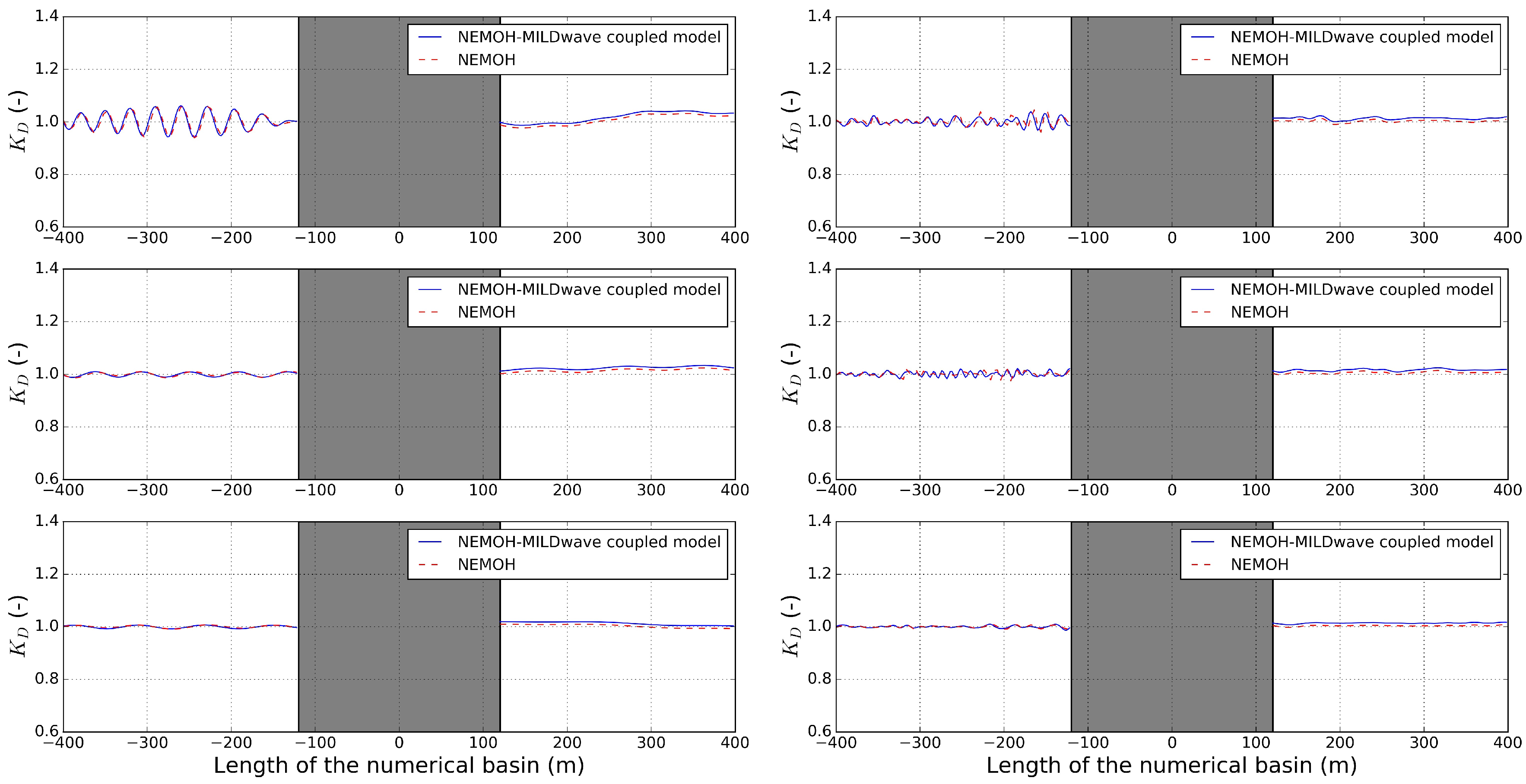
Figure 14.
Cross-section S2 of the for a 9-WEC array at y = 200 m for regular waves (left) and irregular waves (right) for regular waves with T = 6 s, T = 8 s and T = 10 s and for irregular waves with = 6 s, = 8 s and = 10 s.
Figure 14.
Cross-section S2 of the for a 9-WEC array at y = 200 m for regular waves (left) and irregular waves (right) for regular waves with T = 6 s, T = 8 s and T = 10 s and for irregular waves with = 6 s, = 8 s and = 10 s.

Figure 15.
Surface elevations for the NEMOH-MILDwave coupled model and the WECwakes experimental data for a total of 15 wave gauges shown in Figure 8.
Figure 15.
Surface elevations for the NEMOH-MILDwave coupled model and the WECwakes experimental data for a total of 15 wave gauges shown in Figure 8.
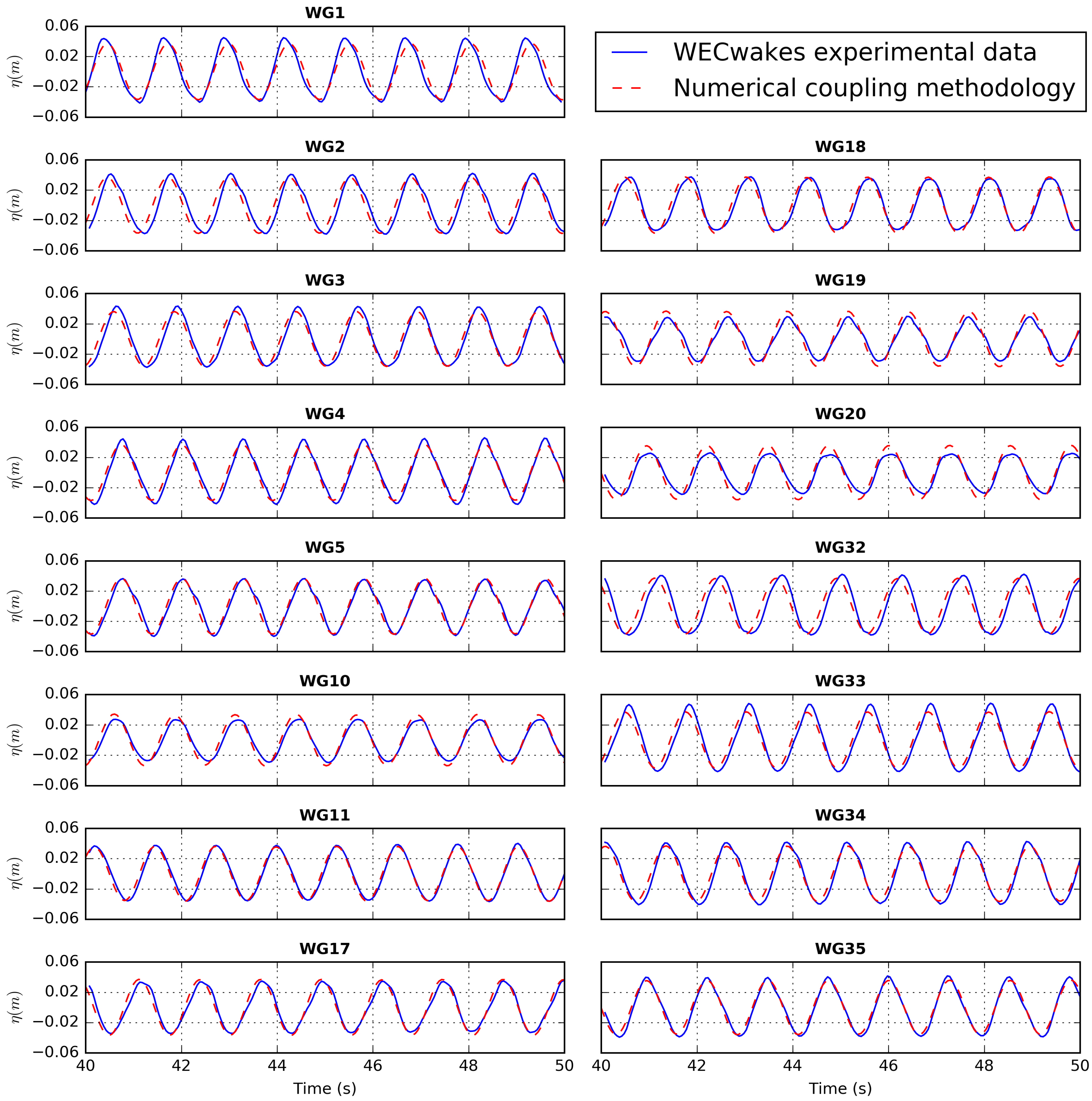
Figure 16.
Root Mean Square Error (RMSE) values for the free surface elevation for the 15 wave gauges analyzed from the data set (see Figure 8).
Figure 16.
Root Mean Square Error (RMSE) values for the free surface elevation for the 15 wave gauges analyzed from the data set (see Figure 8).

Figure 17.
NEMOH-MILDwave couple model values of a 9-WEC array for regular waves (left) with T = 6 s, T = 8 s and T = 10 s and for irregular waves (right) with = 6 s, = 8 s and = 10 s with a slopping bathymetry. Contour levels are set at an interval 0.04 m. Waves are propagating from left to right. The coupling region is masked out with a white circle.
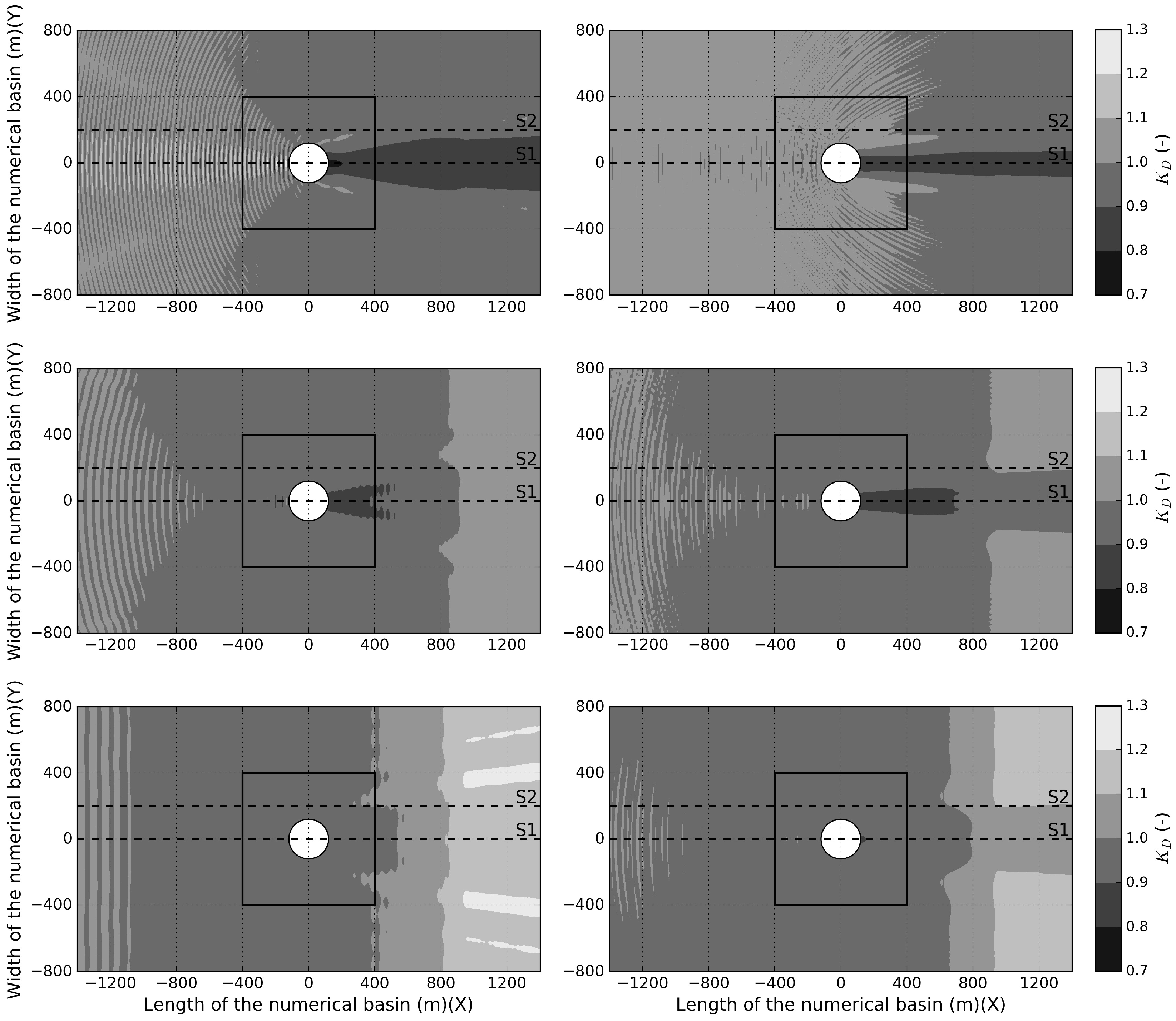
Figure 18.
Cross-section S1 of the for a 9-WEC array at y = 0 m for regular waves (left) with T = 6 s, T = 8 s and T = 10 s and for irregular waves (right) with = 6 s, = 8 s and = 10 s at a constant depth and a sloping bathymetry. The coupling region is masked out in gray between two vertical black lines.


Table 1.
Incident wave data sets used for the coupling methodology test cases.
| Regular Waves | |||
| Case Name | T(s) | H(m) | = 0 |
| A | 6 | 2 | 0 |
| B | 8 | 2 | 0 |
| C | 10 | 2 | 0 |
| Irregular Waves | |||
| Case Name | (s) | (m) | = 0 |
| D | 6 | 2 | 0 |
| E | 8 | 2 | 0 |
| F | 10 | 2 | 0 |
Table 2.
Test program for the coupling methodology implementation in constant bathymetry.
| Test Number | Numerical Models | Wave Type | H (m) | T (s) | Water Depth d (m) |
|---|---|---|---|---|---|
| 1 | NEMOH | REG | 2 | 6 | 40 |
| 2 | NEMOH | REG | 2 | 8 | 40 |
| 3 | NEMOH | REG | 2 | 10 | 40 |
| 4 | NEMOH-MILDwave | REG | 2 | 6 | 40 |
| 5 | NEMOH-MILDwave | REG | 2 | 8 | 40 |
| 6 | NEMOH-MILDwave | REG | 2 | 10 | 40 |
| 7 | NEMOH | IRREG | 2 | 6 | 40 |
| 8 | NEMOH | IRREG | 2 | 8 | 40 |
| 9 | NEMOH | IRREG | 2 | 10 | 40 |
| 10 | NEMOH-MILDwave | IRREG | 2 | 6 | 40 |
| 11 | NEMOH-MILDwave | IRREG | 2 | 8 | 40 |
| 12 | NEMOH-MILDwave | IRREG | 2 | 10 | 40 |
Table 3.
Test program for the coupling methodology implementation in varying bathymetry.
| Test Number | Numerical Models | Wave Type | H (m) | T (s) | Water Depth d (m) |
|---|---|---|---|---|---|
| 13 | NEMOH-MILDwave | REG | 2 | 6 | VAR |
| 14 | NEMOH-MILDwave | REG | 2 | 8 | VAR |
| 15 | NEMOH-MILDwave | REG | 2 | 10 | VAR |
| 16 | NEMOH-MILDwave | IRREG | 2 | 6 | VAR |
| 17 | NEMOH-MILDwave | IRREG | 2 | 8 | VAR |
| 18 | NEMOH-MILDwave | IRREG | 2 | 10 | VAR |
© 2018 by the authors. Licensee MDPI, Basel, Switzerland. This article is an open access article distributed under the terms and conditions of the Creative Commons Attribution (CC BY) license (http://creativecommons.org/licenses/by/4.0/).
Share and Cite
MDPI and ACS Style
Verao Fernandez, G.; Balitsky, P.; Stratigaki, V.; Troch, P. Coupling Methodology for Studying the Far Field Effects of Wave Energy Converter Arrays over a Varying Bathymetry. Energies 2018, 11, 2899. https://doi.org/10.3390/en11112899
AMA Style
Verao Fernandez G, Balitsky P, Stratigaki V, Troch P. Coupling Methodology for Studying the Far Field Effects of Wave Energy Converter Arrays over a Varying Bathymetry. Energies. 2018; 11(11):2899. https://doi.org/10.3390/en11112899
Chicago/Turabian StyleVerao Fernandez, Gael, Philip Balitsky, Vasiliki Stratigaki, and Peter Troch. 2018. "Coupling Methodology for Studying the Far Field Effects of Wave Energy Converter Arrays over a Varying Bathymetry" Energies 11, no. 11: 2899. https://doi.org/10.3390/en11112899
Note that from the first issue of 2016, this journal uses article numbers instead of page numbers. See further details here.