Energy Sustainability in Smart Cities: Artificial Intelligence, Smart Monitoring, and Optimization of Energy Consumption


1
Department of Electronic Engineering, City University of Hong Kong, Hong Kong SAR, China
2
School of Business & Economics, Deree College—The American College of Greece, Gravias 6, 153 42 Aghia Paraskevi, Greece
3
Effat College of Engineering, Effat University, P.O. Box 34689, Jeddah 21478, Saudi Arabia
4
Effat College of Business, Effat University, P.O. Box 34689, Jeddah 21478, Saudi Arabia
*
Author to whom correspondence should be addressed.
Energies 2018, 11(11), 2869; https://doi.org/10.3390/en11112869
Submission received: 10 October 2018
/
Revised: 16 October 2018
/
Accepted: 19 October 2018
/
Published: 23 October 2018
(This article belongs to the Special Issue Artificial Intelligence for Smart and Sustainable Energy Systems and Applications)
Abstract
:Energy sustainability is one of the key questions that drive the debate on cities’ and urban areas development. In parallel, artificial intelligence and cognitive computing have emerged as catalysts in the process aimed at designing and optimizing smart services’ supply and utilization in urban space. The latter are paramount in the domain of energy provision and consumption. This paper offers an insight into pilot systems and prototypes that showcase in which ways artificial intelligence can offer critical support in the process of attaining energy sustainability in smart cities. To this end, this paper examines smart metering and non-intrusive load monitoring (NILM) to make a case for the latter’s value added in context of profiling electric appliances’ electricity consumption. By employing the findings in context of smart cities research, the paper then adds to the debate on energy sustainability in urban space. Existing research tends to be limited by data granularity (not in high frequency) and consideration of about six kinds of appliances. In this paper, a hybrid genetic algorithm support vector machine multiple kernel learning approach (GA-SVM-MKL) is proposed for NILM, with consideration of 20 kinds of appliance. Genetic algorithm helps to solve the multi-objective optimization problem and design the optimal kernel function based on various kernel properties. The performance indicators are sensitivity (Se), specificity (Sp) and overall accuracy (OA) of the classifier. First, the performance evaluation of proposed GA-SVM-MKL achieves Se of 92.1%, Sp of 91.5% and OA of 91.8%. Second, the percentage improvement of performance indicators using proposed method is more than 21% compared with traditional kernel. Third, results reveal that by keeping different modes of electric appliance as identical class label, the performance indicators can increase to about 15%. Forth, tunable modes of GA-SVM-MKL classifier are proposed to further enhance the performance indicators up to 7%. Overall, this paper is a bold and novel contribution to the debate on energy utilization and sustainability in urban spaces as it integrates insights from artificial intelligence, IoT, and big data analytics and queries them in a context defined by energy sustainability in smart cities.
1. Introduction
Cities are the major consumers of electricity today. Considering the correlation that exists between energy consumption, the environmental footprint it leaves, and the implications for and of global warming [1,2], energy sustainability emerges as one of the key questions that beholds the stakeholders, including the industry, decision-makers and the society. Consensus has emerged that replacing old electrical infrastructure by smart grid might be the most effective way of addressing the challenge worldwide. Microgrid applications like transactive energy framework [3,4], energy management [5,6,7] and advanced retail electricity market [8], play an important role in context of smart grid development. Microgrids are typically supported by generators or renewable wind and solar energy resources and are often used to provide backup power or to supplement the main power grid during periods of heavy demand. A microgrid strategy that integrates local wind or solar resources can provide redundancy for essential services and make the main grid less susceptible to localized disaster. Smart metering is one of the key features that conditions the functioning of a smart grid [9]. By 2020, worldwide, the estimated number of smart meters will exceed 800 million, while the penetration rate will be 50% [10,11]. The question is to what extent and how smart metering may contribute to attaining greater efficiency of a smart grid, e.g., by optimizing it. To address this question, this paper employs advances in artificial intelligence and big data analytics to query in which ways their integrated use in context of smart metering and smart grid optimization may yield positive results in the form of decreased energy consumption and greater energy sustainability. Inserting the discussion in context of smart cities, adds an additional twist to this discussion. The argument is structured as follows. In the first section, a review of load monitoring methods is discussed briefly to highlight the value added of non-intrusive load monitoring. Next, the research methodology is outlined, which is followed by overview of empirical testing and analysis. Section 5 evaluates the performance of proposed method and its comparison with related work. Finally a conclusion is drawn.
2. Related Works—Non-Intrusive Load Monitoring (NILM) and Its Value Added
The evolution of modern advanced computational forecasting methods provides new tools for electricity forecasting and pattern recognition. According to individual smart data and smart metering techniques will have a great impact in the efficiency of smart energy solutions. In addition, artificial intelligence techniques and smart grid approaches can set up sophisticated services for the optimization of energy consumption. Toward this direction advanced demand modelling using machine learning algorithms will offer new predicting capabilities. Furthermore, Big Data context increases the complexity of the problem and also requires novel mining techniques based on energy time series for behavioral analytics. Therefore, user behavior and analysis is directly linked, as is integrated behavioral analytics and smart energy modelling, metering and solutions.
Recent research focused on intrusive load monitoring (ILM) and non-intrusive load monitoring (NILM). A study concluded that load monitoring can reduce 20% electricity consumption [12]. In contrast, ILM is distributed sensing, whereas NILM is single-point sensing. ILM uses more than one smart meter per apartment (could be one smart meter per power outlet), but NILM uses only one smart meter in the apartment. Theoretically, more smart meters can yield higher accuracy for the detection of appliance consumption, because the number of appliances that need to be disaggregated is lower [13]. However, disadvantages exist. These include: High cost, complex smart metering network configuration, and management. This paper focuses specifically on NILM and its value added.
Figure 1 shows the general architecture of NILM for electricity suppliers, companies and users. The NILM benefits to electricity suppliers, manufacturers and users. Electricity suppliers can achieve a more accurate demand response by understanding the electricity consumption profile of each electric appliance. Therefore, a better energy demand prediction model can be achieved using the usage pattern. Furthermore, it tries to lower the gap between total electricity supply and demand, in other words, the electricity wastage attributable to unused electricity decreases (it is worth mentioning that the energy supply is always larger than energy demand to ensure it can still fulfill the demand requirement if abrupt increase in demand occurs). For manufacturers, they would be able to develop a better understanding of the relationship between appliances and their usage patterns. One may focus on increasing the energy efficiency of frequently used and power hungry appliances. Last, the electricity consumption pattern of each appliance may correct the misunderstanding of end users whom normally have no idea on electricity consumption. They can formulate a direction to reduce the electricity bill, especially in power hungry appliance.
Various approaches for NILM have been proposed. For instance, decision tree [14,15], graph signal processing [16], hidden Markov model [17,18], k-nearest neighbor [19], clustering [20] and cepstrum-smoothing [21]. It can be seen that the detection interval for some works is not real-time, 8 s in [15] and 1 min in [16,17,18,20]. This is often impractical because the actual operation time for an electric appliance is usually not a divider of 1-min or 8 s. When it comes to NILM, unsupervised or supervised classification is required. It is invalid to define the class label when the operation time is not a divider of the detection interval. Thus, a real-time detection interval 50 Hz or 60 Hz is required, which depends on the line voltage standard of the district. The works in [16,20,21] adopt detection interval of 60 Hz, 50 Hz and 0.5 s respectively. However, these works focused on NILM of 4 or 6 electric appliances, which are far from adequate in the practical situation. The details of [16,17,18,19,20,21], as well as comparison between proposed work and these works will be discussed in Section 5.5.
In this paper, a hybrid generic algorithm support vector machine multiple kernel learning (GA-SVM-MKL) approach has been proposed for NILM of 20 electric appliances. Genetic algorithm helps to solve the multi-objective optimization problem and design the optimal kernel function based on various kernel properties. SVM is adopted owning to the fact that it takes key advantages in (i) avoid over-fitting; (ii) kernel trick; (iii) convex optimization problem; and (iv) good out-of-sample generalization. The contribution is as follows (i) GA-SVM-MKL is capable of analyzing and disaggregating the energy profile of single point into list of 20 common types of operating electric appliances, which is far more than that in existing works; (ii); GA-SVM-MKL achieves Sensitivity (Se) of 92.1–98.4%, Specificity (Sp) of 91.5–98.8% and overall accuracy (OA) of 91.8–98.6% and (iii) Tunable modes of GA-SVM-MKL is introduced to enhance the classification performance by 7% because we can reduce the number of types of appliances in certain period in order to reduce the complexity of model and thus increase the performance of classification model.
3. Research Methodology and Research Problem Formulation
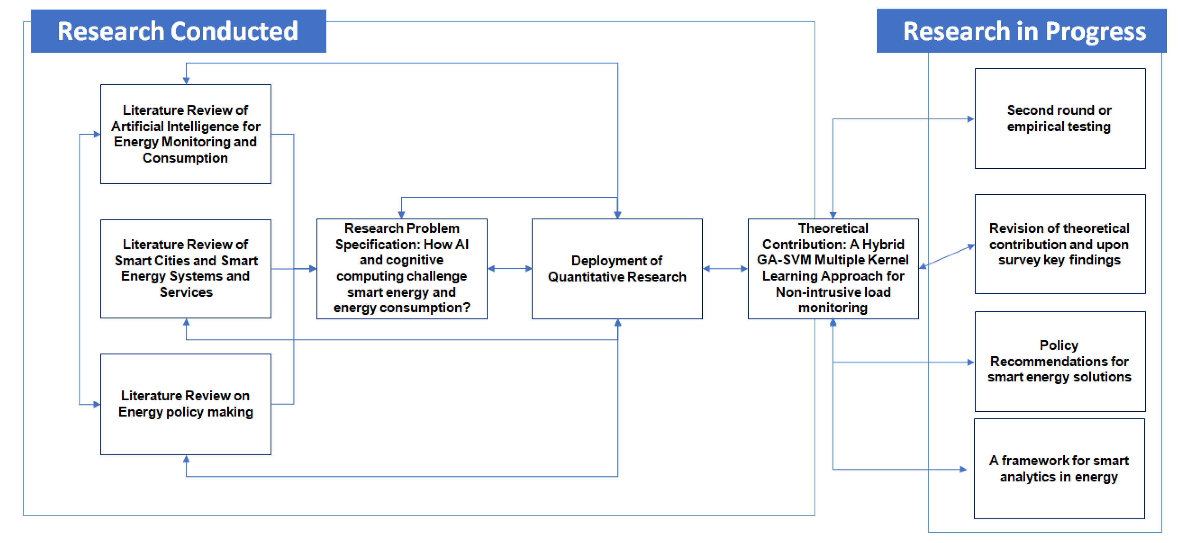
This paper examines to what extent and how smart metering may contribute to attaining greater efficiency of smart grid, for example by optimizing it by deploying advances from the fields of artificial intelligence and big data analytics. To address this question, several hypotheses have been made, as well as corresponding research, including literature review and primary research. Figure 2 depicts the methodology and the workflow. In brief, the research presented here draws from insights from three converging fields of scientific inquiry to rethink the question of smart grid optimization. These insights include:
- Insights from artificial intelligence (AI) and cognitive computing and the value added they bring into the process of designing, managing and utilizing smart energy systems
- Insights from smart cities and smart villages research, as well as considerations specific to the debate on sustainability, including the SDGs, and their value added consistent with an emphasis on wellbeing and inclusive socio-economic growth and development
- Insights from the broad field pertinent to energy supply and demand and related questions the value added if ICT-driven coherent and effective policymaking
It is at the intersection of these three broad domains that our research question is located. Accordingly, the more specific research questions that this paper will address include: In which ways novel ICT-enhanced solutions, including algorithms and data integration, can contribute to efficient and sustainable consumption of resources, like energy.
“What is the optimal design of classification model for NILM application”. The multiple objectives optimization problem will be solved by multi-objective genetic algorithm.
“Can we reduce the number of types of appliances in certain period in order to reduce the complexity of model and thus increase the performance of classification model”. This will be addressed in Section 5.4.
4. Overview of Empirical Testing and Analysis
The general flow of GA-SVM-MKL classifier for NILM is given in Figure 3. The smart meter will measure the current and voltage waveform of the apartment continuously. Both waveforms are carried out signal preprocessing includes dc offset elimination, interval segmentation. In this paper, 0.2 s interval is selected as of the line voltage standards in Hong Kong, 220 V/50 Hz. Features of each interval segment are then computed. The features act as input for the embedded and trained GA-SVM-MKL classifier. The training of classifier includes signal preprocessing and features extraction. Then, formulation of different multi-objective SVM classifiers is carried out by various combinations of typical kernels. The multi-objective optimization problems are solved by genetic algorithm. The optimal designs of classifier under different combinations of typical kernels can be concluded. It is worth mentioning that a well-known 10-fold cross-validation is adopted for the training of classifier [22,23,24]. The outputs of the classifier are types of operating electric appliances and electricity consumption of operating electric appliances. Based on the outputs of the classifier, three major applications, billing, demand response and appliance usage pattern can be obtained. Electricity suppliers may utilize all applications whereas companies and end users may only utilize the appliance usage pattern.
This section comprises of three subsections. First, the measurement and preparation of datasets for training and validation of GA-SVM-MKL classifier are discussed. Second, possible features for constructing the GA-SVM-MKL classifier are presented. At last, the formulation of optimal design of GA-SVM-MKL classifier is explained.
4.1. Datasets of Electric Appliances
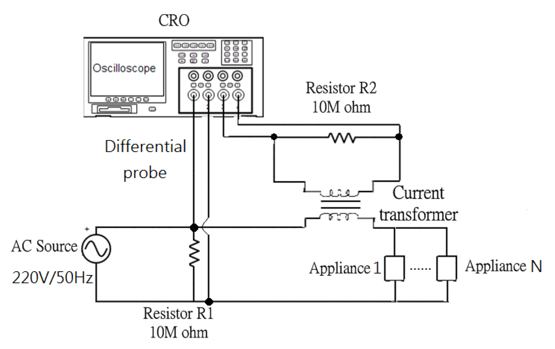
Figure 4 shows the measurement set up for obtaining the voltage and current waveforms of all electric appliances. The voltage of 220 Vrms is measured with differential probe using cathode ray oscilloscope (CRO) with sampling frequency Fs = 10 kHz. A current transformer with ratio 50/5 is utilized for measuring the current waveform. The resistor R1 is chosen to be large value (10 MΩ), which because it has negligible effect to the circuit. The resistor R2 of 10 MΩ is connected in series with the secondary winding of current transformer to avoid open circuit.
The datasets consist of 20 electric appliances that are commonly used in typical households. The measurement allows multiple operation of electric appliances, in other words, the current waveforms may be superimposed by multiple electric appliances. Table 1 summarizes the electric appliances along with their type of activity, modes and number of brands being considered. The electric appliances can be divided into six activities, lighting, cooking, home living, computing, renovating and audio and video. There is limitation that the measurement cannot cover all brands of each electric appliance, each electric appliance has at least two brands for consideration. Likewise, there is a maximum number for each electric appliance operating at any instant in a typical household. For every combination of electric appliances, the corresponding voltage and current waveforms are recorded for 30 s (equivalent to 30 × 50 = 1500 samples). Each combination is assigned with a unique class label. It is noted that in Section 5.1, different modes of electric appliances will be assumed as identical class label and that in Section 5.2 will be assumed as different class labels.
After measuring the voltage and current waveforms of electric appliances, the waveforms perform dc offset elimination, whichIndividual samples can be obtained by segmentation of signals with interval of 0.2 s.
4.2. Features Extraction
F The individual samples I(n) and V(n) are transformed to feature vector. The proposed GA-SVM-MKL adopts seven features: Maximum current (Imax), root-mean-square current (Irms), average current (Iavg), active power (Pact), apparent power (Papp), reactive power (Prea) and power factor (PF). The features can be computed by:
It is worth mentioning that dimensionality reduction (e.g., in [11]) is not adopted because all of these features are essential for distinguishing between electric appliances in nature. The focus will be devoted on the optimal design of kernel function for building SVM classifier.
4.3. Optimal Design of GA-SVM-MKL Classifier
Denote electric appliances samples by Xij(n) with current Iij(n) and Vij(n) for class i = 1,…,Nc and j = 1,…,Ni where Ni = 1500 is the total number of samples in class i. Let feature vector be fij = {Imax,ij, Irms,ij, Iavg,ij, Pact,ij, Papp,ij, Prea,ij, PFij} corresponds to Xij(n).
When it comes to the selection of kernels, there are five typical kernels k(x1, x2) with inner product 〈x1,x2〉. They are linear kernel, qth degree polynomial kernel, complete polynomial kernel, radial basis function (RBF) kernel and sigmoid kernel. The expressions of these kernels can be summarized as follows:
where .
Different kernels possess different characteristics where there is no single kernel that works well in all applications. In this paper, the proposed GA-SVM-MKL classifier adopts the idea that by combining multiple kernels (namely multiple kernel learning), the classifier can achieve better performance for NILM after taking the advantages from each kernel. In order to combine kernels to form a new one, the kernel should obey Mercer’s Theorem. According to [25], there are four properties (P):
where and are any two Mercer kernels. It is noted that properties 1 and 4 can be further extended to infinite number of Mercer kernels.
The optimal design of classifier for NILM is formulated as a multi-objective optimization problem and solved by genetic algorithm. Multi-objective optimization is an integral part of optimization activities and has tremendous practical importance, since almost all real-world optimization problems are ideally suited to be modeled using multiple conflicting objectives [26]. Compared with single objective optimizations, which usually scalarizing multiple-objectives into one single objective, multi-objective optimization can give trade-off optimal solutions more accurately. Besides, the multi-objective optimization has multiple cardinalities of the optimal set, multiple objectives and different search spaces [27]. The objective functions constitute a multidimensional space, which is known as objective spaces [28]. The optimal solutions presented in objective spaces are referred to as Pareto optimal solutions and the set of such solutions are called Pareto Front.
As the objectives conflict with each other, it is usually impossible to obtain one single optimal objective. Therefore, for obtaining the optimal solutions in multi-objective optimizations, the most used concept is domination. Assuming for an M-objective minimization problem, candidate solution u is dominated by another candidate solution v if and only if function values of u is partially less than v, which is formulated as [26]:
Based on the concept of domination, what we prefer are the non-dominated solutions, which compose the Pareto Front. In this paper, in order to give the optimal design of classifier for NILM, multi-objective optimization genetic algorithm (MOGA) [27] for solving the multiple kernels is designed. The flow of the MOGA for the optimal design of kernel functions is shown in Figure 5. The procedures are as follows: (i) The population size and values of objective function are initialized; (ii) the values of objective function of individuals in the population are computed using the values of objective function defined in (i); (iii) ranking the individuals according to the values of objective function; (iv) the population convergence is dependent on small group of pareto optimal solutions, but not all optimal solutions attributable to the nature of the stochastic selection errors, given a limited population size; (v) niche count is introduced to enhance the population diversity by lengthening the distance between two optimal solutions along the axis of objective functions. The convergence to small group solutions will be avoided; (vi) a new offspring is generated and the values of objective functions are evaluated; (vii) ranks assignment and niche count calculation are carried out repeatedly in the new offspring; and (viii) the algorithm is terminated if it attains the maximum number of generations or if the output reaches the pareto front. It is noted that there exist other stopping criteria in literature for stochastic optimization algorithm and can be referred to [29,30,31].
The multi-objective optimization problem for NILM can be formulated as:
where Se is the sensitivity of the classifier, Sp is the specificity of the classifier, is a margin equals to distance of closest samples from the hyperplane, is the Lagrange multiplier and is the output of the classifier. The three objective functions Se, Sp and are defined as:
where TP is the number of true positive samples, TN is the number of true negative samples, Np is the total number of positive samples, Nn is the total number of negative samples. The customized and optimized kernel for NILM, kNILM varies by different combination of typical kernels in (8)–(12) using Properties 1–4 in (13)–(16). These scenarios are summarized in Appendix A Table A1, which have been studied and analyzed. It is noted that due to there are infinite scenarios settings, only property combinations of property (P), P1, P2, P3, P4, P1P2, P1P3, P1P4, P1P5, P2P3, P2P4, P2P5, P3P4, P3P5, P4P5 are illustrated and analyzed. These 285 scenario settings cover adequate analysis for taking the advantages from individual kernel to form a multiple kernel for kNILM.
The proof of combinations of property P1P2, P1P3, P1P4, P1P5, P2P3, P2P4, P2P5, P3P4, P3P5, P4P5 is shown below:
For all and all sequences let K1, K2, K3, K4, KP1P2, KP1P3, KP1P4, KP2P3, KP2P4 and KP2P3 be the r × r matrices whose i, j-th element is given by k1(xi, xj), k2(xi, xj), k3(xi, xj), k4(xi, xj), c1k1(xi, xj) + c2k2(xi, xj), k1(xi, xj) + k2(xi, xj) + c, (k1(xi, xj) + k2(xi, xj))(k3(xi, xj)k4(xi, xj)), c1k1(xi, xj) + c2, ck1(xi, xj)k2(xi, xj) and (k1(xi, xj) + c)k2(xi, xj) respectively. It is required to show that KP1P2, KP1P3, KP1P4, KP2P3, KP2P4 and KP2P3 are positive semidefinite using only that K1, K2, K3 and K4 are positive semidefinite, i.e., for all , , , and .
(iii) The r2 × r2 matrix and are positive semidefinite, that is, for all , and . Given any , consider . Then
Similarly, it can be derived that
Thus,
5. Performance Evaluation and Comparisons
This section is divided into five subsections. Section 5.1 discusses the performance of the proposed GA-SVM-MKL classifiers. In Section 5.2, in order to show the effectiveness of kNILM using multiple kernels, the performance of classifier using kNILM is compared with either single kernel is used. The feasibility study of breaking down electric appliances into different modes is discussed in Section 5.3. Intuitively, some activities like cooking and renovating are carried out in certain period. Thus, the number of classes for classifier can be reduced when these electric appliances are not in-use and the classifier is then retrained. Results in Section 5.4 support this hypothesis. Finally, comparison between proposed GA-SVM-MKL classifier and related works is carried out in Section 5.5.
5.1. Performance Evaluation of GA-SVM-MKL Classifier
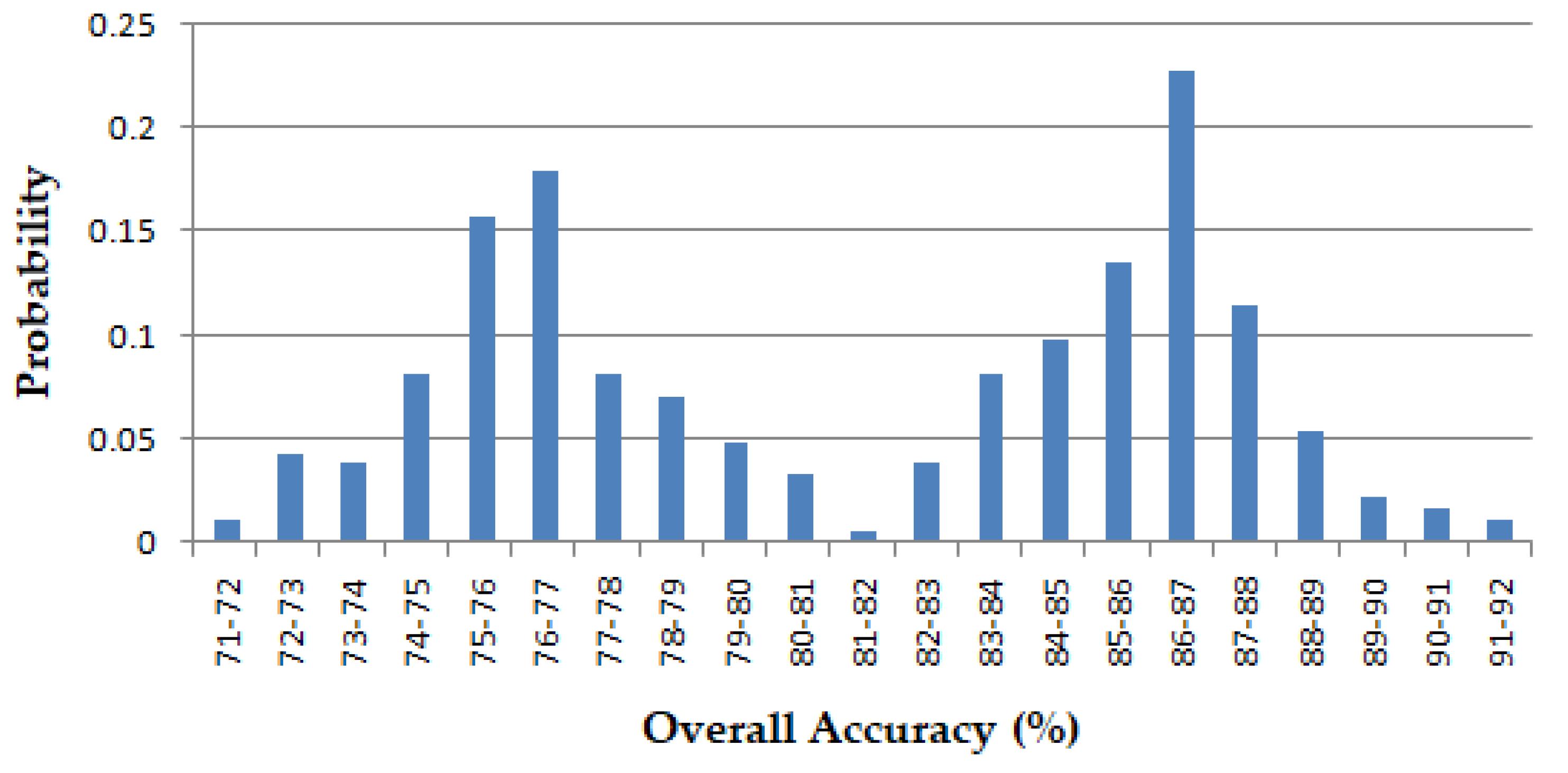
285 scenarios for kNILM using P1, P2, P3, P4, P1P2, P1P3, P1P4, P2P3, P2P4 and P3P4, with typical kernels k1, k2, k3, k4 and k5 are optimally designed. The Se, Sp and overall accuracy (OA) of the GA-SVM-MKL in each scenario are recorded as shown in Appendix A Table A2. OA is defined as the average of Se and Sp given that the identical sample size in each class of the classifier. Probability distribution of the OAs for 285 scenarios is shown in Appendix A, as in Figure A1. The skewness and kurtosis of the OA for all scenarios are −0.0902 (left skewed) and 1.547 (heavy-tailed) respectively.
All results are obtained using 10-fold cross-validation. Scenario 178 using P1P2 achieves the best performance with Se of 92.1%, Sp of 91.5% and OA of 91.8%. The average OA using different properties can be ranked by OAP2P3 > OAP3P4 > OAP2P4 > OAP1P2 > OAP1P3 > OAP1P4 > OAP2> OAP1 > OAP3 > OAP4 with accuracies 87.3%, 86.7%, 85.8%, 83.4%, 76.7%, 76.6%, 75.8%, 75.6%, 75.3%, and 74.7% respectively.
Results reveal that merging kernel properties and adopting multiple kernel learning can achieve better performance than using single property.
5.2. Comparisons to Single Kernel Based SVM Classifier
The performance of proposed GA-SVM-MKL classifier is compared to traditional SVM classifier using single kernel k1, k2, k3, k4 and k5. It is noted that this SVM classifier deals with single objective maximization problem, which maximizes the margin which has been defined in (22). The comparison is shown in Table 2. The proposed GA-SVM-MKL classifier increases the Se, Sp and OA by 21.3–28.6%, 21.5–26.7% and 21.4–27.7% respectively. Among five scenarios using traditional SVM with k1–k5, the best performance is using k4, which follows by k5, k3, k2 and k1. The better performance of proposed GA-SVM-MKL can be explained by two reasons. First, GA-SVM-MKL adopts optimal kernel using multiple kernel learning with kernel properties in which it takes the advantages from each individual kernel for customization to NILM. Second, traditional SVM aims at single objective optimization, which maximizes the margin, but not Se and Sp.
5.3. Feasibility Study of Assignment a Class Label for Different Modes of Electric Appliance
Among 20 electric appliances in this study, seven electric appliances, electric stove, microwave oven, cooker, ironbrush, fan, hair dryer and electric heater have more than one mode. These are activities of cooking and home living. In Section 5.1, it is assumed that different modes of the same electric appliances are of the same class. In this section, analysis has been made to assign different modes of the same electric appliances to be different classes. Thus, the 20 electric appliances can be extended to 32 electric appliances. Table 3 shows four scenarios S1, S2, S3 and S4 for the performance comparisons of GA-SVM-MKL classifier between before and after the assignment of new classes.
Compared between S1 and S2, the assignment of new class label for different modes of electric appliances decreases the Se, Sp and OA by 15.7%, 14.4% and 15.0% respectively. Scenarios S3 and S4 reveal that the decrease in Se, Sp and OA are mainly due to the introduction of new class labels for activities of cooking and home living. Therefore, the original assumption that different modes of same electric appliances should be considered as identical electric appliance is verified.
5.4. Tunable Mode for GA-SVM-MKL Classifier
Aforementioned, the 20 electric appliances for study can be divided into six activities, lighting, cooking, home living, computing, renovating and audio and video. All activities except renovating are daily used. For cooking, it is periodic activities in which users turn on the electric appliances in breakfast, lunch or dinner. Thus, it is proposed that GA-SVM-MKL classifier can be tuned for different electric appliances detection with five tunable modes (TMs).
(i) TM 1 assumes a full range classifier, in which all 20 electric appliances in six activities can be detected.
(ii) TM 2 can be selected when it is breakfast, lunch or dinner so that electric appliances of cooking should be detected by the classifier. Provided that there is no renovating, five activities, lighting, cooking, home living, computing and audio and video can be detected.
(iii) TM 3 is a non-eating period where electric appliances of cooking are not necessary. However, there is small-scale renovating activity, which allows normal activities inside the house. Five activities, including lighting, home living, computing, renovating, and audio and video, can be detected.
(iv) TM 4 assumes electric appliances related to cooking and renovating activities will not be operated. Only four activities, lighting, home living, computing and audio and video will be operated and detected.
(v) TM 5 assumes a large-scale renovating, in which only electric appliances of renovating (1 activity) are detected.
Table 4 summarizes the modes and the activities of GA-SVM-MKL classifier. For each mode, a GA-SVM-MKL classifier is trained using 10-fold cross-validation. Practically, end users can enter the period for breakfast, lunch and dinner during weekday and weekend so that GA-SVM-MKL classifier can detect electric appliances of cooking in specific time interval. Also, the ability to detect electric appliances of renovating is turned off until end users specify there is a renovation activity in their apartment.
The Se, Sp and OA for the classifier in TM 1 to 5 have been recorded in Table 5. A finding is observed, the Se, Sp and OA of the classifier increase when the number of activities (or classes) decreases. This may be explained by fewer classes, the classification problem is less complex. Thus, it is shown that the proposed mode tunable GA-SVM-MKL classifier can help improving the Se, Sp and OA for NILM. Compared between TM1 and TM2-TM5, the percentage improvement using tunable mode is ranged (1.85%, 6.84%), (2.84%, 7.98%), (2.51%, 7.41%) for Se, Sp and OA respectively.
5.5. Comparisons to Related Works
Related works for NILM include different methods like decision tree [14,15], graph signal processing [16], hidden Markov model [17,18], k-nearest neighbor [19], clustering [20] and cepstrum-smoothing [21]. The features, datasets, cross-validation, detection interval, and OA of each method have been summarized in Table 6. It should be noted that related work in [18] focused on building a probabilistic appliance model which has been generalized to match previously unseen households; thus, it did not involve any classifier for NILM.
It can be seen that the existing works [15,16,17,20] using detection interval of 8 s or 1-min interval, which is far from using real-time data. There are two concerns for using these detection intervals. First, the operation time of electric appliances is generally not a divider of 8 s or 1-min. It is difficult to define the class label. On the other hand, it increases the difficulty for the classification, because (i) detection interval of 8 s, researchers are expected to find out whether the actual operation time of electric appliance is 1 s, 2 s, … or 8 s. (ii) detection interval of 1-min, likewise, the determination of operation time of electric appliance equals 1 s, 2 s, … or 60 s is required. Thus, related works in [15,16,17,20] achieve Se, Sp and OA less than 80%.
The detection intervals in [14,19,21] are 60 Hz, 0.5 s and 50 Hz respectively. For OA, these works achieve 96.65% [14], 94.87% [19] and 96.37% [21]. However, these works only consider the NILM of 4 or 6 electric appliances, which is much less than that in this paper (20 electric appliances). Also, previous works are lack of or without mentioned one of the most important part in the performance evaluation, cross-validation. One can pick up a bias training dataset to train the classifier so that the results are not convincing and reliable. In aforementioned related works, Se and Sp are not given, which is believed to be important criteria to evaluate both the accuracies in determining the true positive and true negative samples. It is noted that when Se and Sp are far from each other, the chance of having bias in some classifiers (toward specific classes) is high.
By comparing the GA-SVM-MKL TM 1-TM5 with [14,19,21] their OAs are similar. Thus, it can be concluded that the proposed method achieves good performance in NILM when the number of electric appliances is extended to 20.
We have to comment on the adoption of this method in the real world. Smart metering on real time basis is quite complicated research problem. The evolution of machine learning techniques along with real time sensors and big data capabilities will increase our capacity to model, meter and analyze behavioral patterns over energy consumption. This will help us a lot to understand the linkages between behavior and energy consumption. From a decision support point of view, irrelevant of the programing and development environments, e.g., smart grid, the key challenge is to be capable of aggregating smart energy data for advanced computational processing. Within this context some of the most challenging future research directions can be:
- Standardization of Smart Energy data sets;
- Interoperability in the Energy Smart Grid;
- Adoption of machine learning techniques for the provision and measurement of Behavioral analytics;
- Integration of Smart Grid approaches in Energy Sector with a new era of Key Performance Indicators (KPIs) and Energy Analytics;
- Large scale experimentation with millions of electrical devices for pattern analysis;
- Optimization of electricity consumption on real time basis based on smart energy data;
- Ontological Engineering and Semantic Annotation of smart energy data.
6. Conclusions
Considering the energy sustainability challenge cities/urban areas are exposed to today, the objective of this paper was to examine ways of optimizing the use of electricity consumption and suggest ways of employing these solutions in cities’/urban areas’ context. Specifically, the research presented in this paper focused on the question of to what extent and how smart metering may contribute to attaining greater efficiency of smart grid. The hypothesis underlying the research was that an integrated approach consistent with engaging insights from (i) artificial intelligence, cognitive computing and big data analytics, (ii) smart cities and smart villages research, and (iii) energy sustainability debate, may yield novel findings. In fact, having employed a complex methodology, as a result of research discussed in this paper a genetic algorithm support vector machine multiple kernel learning (GA-SVM-MKL) approach has been proposed for NILM. A customized kernel has been designed using typical kernel functions with kernel properties. This approach is customized to specific problem, which is NILM for energy disaggregation. Applying kernel properties in various types of kernels can increase the performance of the classifier. Three objective functions have been solved for the optimal design of the classifier to detect 20 common household electric appliances with five tunable modes. The effectiveness of GA-SVM-MKL has been demonstrated. To this end, (i) 20 common types of of electric appliances have been considered, which is far more than that in existing works (at most 10 as in Table 6); (ii) it achieves Se of 92.1–98.4%, Sp of 91.5–98.8% and OA of 91.8–98.6%; and (iii) tunable modes of GA-SVM-MKL is introduced to enhance the classification performance by 7%.
The authors are aware of the limitations of this research. The consideration of the number of types of appliance, the number of modes and brands, as well as the maximum number of appliance is limited. The coverage of the dataset could be extended when it comes to large-scale study. In addition, investigation of the feature extraction could be one of the solutions to further improve the accuracy of the classifier.
The contribution of this paper to the research agenda outlined in the Special Issue titled Artificial Intelligence for Smart Grid is multifold:
First, from a technical point of view it demonstrates the capacity of AI techniques to model complex problems and to simulate optimized solutions. Furthermore, it proves the new era of computational problems where the creation and consumption of big data requires efficient and coherent approaches integrating IoT, big data analytics and AI algorithms:
- Insights from artificial intelligence (AI) and cognitive computing and the value added they bring into the process of smart systems [32]
Second, from a strategic management and sustainability point of view, this paper heralds the onset of a new era of energy-focused data-driven decision-making. This new era defined by the imperative of energy sustainability requires dynamic real time distributed infrastructure and techniques to manage and utilize data flows from millions of devices (IoT), It also requires high speed networks that can bring together all stakeholders, including energy produces, providers, businesses, end-users, decisionmakers. This suggests that new research is needed that would focus on the question of how blockchain technology may effectively serve this role [37]. Indeed, this is subject of our research in-progress.
Additionally, the decision-making point of view, the arguments outlined in this paper suggest that more attention needs to be devoted to the work in progress undertaken by key stakeholders involved in efforts geared toward optimizing electricity consumption. This includes the key electric appliances producers, as well as key actors involved in devising regulatory frameworks, incl. the Organization for Economic Cooperation and Development (OECD) and the European Union (EU). Arguably, several of actions undertaken by these actors would benefit from the findings discussed in this paper.
In the direction of future research, several interesting new research areas promote the interdisciplinary nature of sustainable smart energies research: Based on [38,39] the evolution of individual smart data and smart metering techniques together with advanced Artificial Intelligence and Machine Learning approaches will set up new challenges for intelligent energy agents. Sophisticated and complicated modelling of energy consumption will also allow new analytical processing and predicting capabilities [38]. The evolution of Data Mining, multidimensional data based and distributed DataWarehouses, together with Cloud Services will promote the vision of Enengies’ Software, Platform and Infrastructure as a Service [39,40]. In this direction, user behavior and a behavioral analysis is directly linked, as is integrated behavioral analytics and smart energy modelling, metering and solutions [41]. We plan very shortly to present a global survey on the social impact of Big Data for Sustainable Energy.
Author Contributions
Conceptualization, K.T.C., M.D.L. and A.V.; Methodology, K.T.C.; Validation, K.T.C., M.D.L. and A.V.; Formal Analysis, K.T.C.; Writing-Original Draft Preparation, K.T.C., M.D.L. and A.V.; Writing-Review & Editing, K.T.C., M.D.L. and A.V.
Funding
This research received no external funding. M.D.L. and A.V. would like to thank Effat University in Jeddah, Saudi Arabia, for offering resources for conducting research through the Research and Consultancy Institute.
Conflicts of Interest
The authors declare no conflict of interest.
Appendix A

Table A1.
Scenario setting for kNILM using properties 1–4 with typical kernels.
| No. | P | kNILM | No. | P | kNILM | No. | P | kNILM | No. | P | kNILM | No. | P | kNILM |
|---|---|---|---|---|---|---|---|---|---|---|---|---|---|---|
| 1 | 1 | k1 + k1 | 2 | 1 | k1 + k2 | 3 | 1 | k1 + k3 | 4 | 1 | k1 + k4 | 5 | 1 | k1 + k5 |
| 6 | 1 | k2 + k2 | 7 | 1 | k2 + k3 | 8 | 1 | k2 + k4 | 9 | 1 | k2 + k5 | 10 | 1 | k3 + k3 |
| 11 | 1 | k3 + k4 | 12 | 1 | k3 + k5 | 13 | 1 | k4 + k4 | 14 | 1 | k4 + k5 | 15 | 1 | k5 + k5 |
| 16 | 2 | ck1 | 17 | 2 | ck2 | 18 | 2 | ck3 | 19 | 2 | ck4 | 20 | 2 | ck5 |
| 21 | 3 | k1 + c | 22 | 3 | k2 + c | 23 | 3 | k3 + c | 24 | 3 | k4 + c | 25 | 3 | k5 + c |
| 26 | 4 | k1k1 | 27 | 4 | k1k2 | 28 | 4 | k1k3 | 29 | 4 | k1k4 | 30 | 4 | k1k5 |
| 31 | 4 | k2k2 | 32 | 4 | k2k3 | 33 | 4 | k2k4 | 34 | 4 | k2k5 | 35 | 4 | k3k3 |
| 36 | 4 | k3k4 | 37 | 4 | k3k5 | 38 | 4 | k4k4 | 39 | 4 | k4k5 | 40 | 4 | k5k5 |
| 41 | 1.2 | c1k1 + c2k2 | 42 | 1.2 | ck1 + k2 | 43 | 1.2 | k1 + ck2 | 44 | 1.2 | c1k1 + c2k3 | 45 | 1.2 | ck1 + k3 |
| 46 | 1.2 | k1 + ck3 | 47 | 1.2 | c1k1 + c2k4 | 48 | 1.2 | ck1 + k4 | 49 | 1.2 | k1 + ck4 | 50 | 1.2 | c1k1 + c2k5 |
| 51 | 1.2 | ck1 + k5 | 52 | 1.2 | k1 + ck5 | 53 | 1.2 | c1k2 + c2k3 | 54 | 1.2 | ck2 + k3 | 55 | 1.2 | k2 + ck3 |
| 56 | 1.2 | c1k2 + c2k4 | 57 | 1.2 | ck2 + k4 | 58 | 1.2 | k2 + ck4 | 59 | 1.2 | c1k2 + c2k5 | 60 | 1.2 | ck2 + k5 |
| 61 | 1.2 | k2 + ck5 | 62 | 1.2 | c1k3 + c2k4 | 63 | 1.2 | ck3 + k4 | 64 | 1.2 | k3 + ck4 | 65 | 1.2 | c1k3 + c2k5 |
| 66 | 1.2 | ck3 + k5 | 67 | 1.2 | k3 + ck5 | 68 | 1.2 | c1k4 + c2k5 | 69 | 1.2 | ck4 + k5 | 70 | 1.2 | k4 + ck5 |
| 71 | 1.3 | k1 + k1 + c | 72 | 1.3 | k1 + k2 + c | 73 | 1.3 | k1 + k3 + c | 74 | 1.3 | k1 + k4 + c | 75 | 1.3 | k1 + k5 + c |
| 76 | 1.3 | k2 + k2 + c | 77 | 1.3 | k2 + k3 + c | 78 | 1.3 | k2 + k4 + c | 79 | 1.3 | k2 + k5 + c | 80 | 1.3 | k3 + k3 + c |
| 81 | 1.3 | k3 + k4 + c | 82 | 1.3 | k3 + k5 + c | 83 | 1.3 | k4 + k4 + c | 84 | 1.3 | k4 + k5 + c | 85 | 1.3 | k5 + k5 + c |
| 86 | 1.4 | k1k1 + k1 | 87 | 1.4 | k1k1 + k2 | 88 | 1.4 | k1k1 + k3 | 89 | 1.4 | k1k1 + k4 | 90 | 1.4 | k1k1 + k5 |
| 91 | 1.4 | k1k2 + k1 | 92 | 1.4 | k1k2 + k2 | 93 | 1.4 | k1k2 + k3 | 94 | 1.4 | k1k2 + k4 | 95 | 1.4 | k1k2 + k5 |
| 96 | 1.4 | k1k3 + k1 | 97 | 1.4 | k1k3 + k2 | 98 | 1.4 | k1k3 + k3 | 99 | 1.4 | k1k3 + k4 | 100 | 1.4 | k1k3 + k5 |
| 101 | 1.4 | k1k4 + k1 | 102 | 1.4 | k1k4 + k2 | 103 | 1.4 | k1k4 + k3 | 104 | 1.4 | k1k4 + k4 | 105 | 1.4 | k1k4 + k5 |
| 106 | 1.4 | k1k5 + k1 | 107 | 1.4 | k1k5 + k2 | 108 | 1.4 | k1k5 + k3 | 109 | 1.4 | k1k5 + k4 | 110 | 1.4 | k1k5 + k5 |
| 111 | 1.4 | k2k2 + k1 | 112 | 1.4 | k2k2 + k2 | 113 | 1.4 | k2k2 + k3 | 114 | 1.4 | k2k2 + k4 | 115 | 1.4 | k2k2 + k5 |
| 116 | 1.4 | k2k3 + k1 | 117 | 1.4 | k2k3 + k2 | 118 | 1.4 | k2k3 + k3 | 119 | 1.4 | k2k3 + k4 | 120 | 1.4 | k2k3 + k5 |
| 121 | 1.4 | k2k4 + k1 | 122 | 1.4 | k2k4 + k2 | 123 | 1.4 | k2k4 + k3 | 124 | 1.4 | k2k4 + k4 | 125 | 1.4 | k2k4 + k5 |
| 126 | 1.4 | k2k5 + k1 | 127 | 1.4 | k2k5 + k2 | 128 | 1.4 | k2k5 + k3 | 129 | 1.4 | k2k5 + k4 | 130 | 1.4 | k2k5 + k5 |
| 131 | 1.4 | k3k3 + k1 | 132 | 1.4 | k3k3 + k2 | 133 | 1.4 | k3k3 + k3 | 134 | 1.4 | k3k3 + k4 | 135 | 1.4 | k3k3 + k5 |
| 136 | 1.4 | k3k4 + k1 | 137 | 1.4 | k3k4 + k2 | 138 | 1.4 | k3k4 + k3 | 139 | 1.4 | k3k4 + k4 | 140 | 1.4 | k3k4 + k5 |
| 141 | 1.4 | k3k5 + k1 | 142 | 1.4 | k3k5 + k2 | 143 | 1.4 | k3k5 + k3 | 144 | 1.4 | k3k5 + k4 | 145 | 1.4 | k3k5 + k5 |
| 146 | 1.4 | k4k4 + k1 | 147 | 1.4 | k4k4 + k2 | 148 | 1.4 | k4k4 + k3 | 149 | 1.4 | k4k4 + k4 | 150 | 1.4 | k4k4 + k5 |
| 151 | 1.4 | k4k5 + k1 | 15yh72 | 1.4 | k4k5 + k2 | 153 | 1.4 | k4k5 + k3 | 154 | 1.4 | k4k5 + k4 | 155 | 1.4 | k4k5 + k5 |
| 156 | 1.4 | k5k5 + k1 | 157 | 1.4 | k5k5 + k2 | 158 | 1.4 | k5k5 + k3 | 159 | 1.4 | k5k5 + k4 | 160 | 1.4 | k5k5 + k5 |
| 161 | 2.3 | c1k1(k1 + c2) | 162 | 2.3 | c1k1(k2 + c2) | 163 | 2.3 | c1k1(k3 + c2) | 164 | 2.3 | c1k1(k4 + c2) | 165 | 2.3 | c1k1(k5 + c2) |
| 166 | 2.3 | c1k2(k1 + c2) | 167 | 2.3 | c1k2(k2 + c2) | 168 | 2.3 | c1k2(k3 + c2) | 169 | 2.3 | c1k2(k4 + c2) | 170 | 2.3 | c1k2(k5 + c2) |
| 171 | 2.3 | c1k3(k1 + c2) | 172 | 2.3 | c1k3(k2 + c2) | 173 | 2.3 | c1k3(k3 + c2) | 174 | 2.3 | c1k3(k4 + c2) | 175 | 2.3 | c1k3(k5 + c2) |
| 176 | 2.3 | c1k4(k1 + c2) | 177 | 2.3 | c1k4(k2 + c2) | 178 | 2.3 | c1k4(k3 + c2) | 179 | 2.3 | c1k4(k4 + c2) | 180 | 2.3 | c1k4(k5 + c2) |
| 181 | 2.3 | c1k5(k1 + c2) | 182 | 2.3 | c1k5(k2 + c2) | 183 | 2.3 | c1k5(k3 + c2) | 184 | 2.3 | c1k5(k4 + c2) | 185 | 2.3 | c1k5(k5 + c2) |
| 186 | 2.4 | ck1(k1k2) | 187 | 2.4 | ck1(k1k3) | 188 | 2.4 | ck1(k1k4) | 189 | 2.4 | ck1(k1k5) | 190 | 2.4 | ck1(k2k3) |
| 191 | 2.4 | ck1(k2k4) | 192 | 2.4 | ck1(k2k5) | 193 | 2.4 | ck1(k3k4) | 194 | 2.4 | ck1(k3k5) | 195 | 2.4 | ck1(k4k5) |
| 196 | 2.4 | ck2(k1k2) | 197 | 2.4 | ck2(k1k3) | 198 | 2.4 | ck2(k1k4) | 199 | 2.4 | ck2(k1k5) | 200 | 2.4 | ck2(k2k3) |
| 201 | 2.4 | ck2(k2k4) | 202 | 2.4 | ck2(k2k5) | 203 | 2.4 | ck2(k3k4) | 204 | 2.4 | ck2(k3k5) | 205 | 2.4 | ck2(k4k5) |
| 206 | 2.4 | ck3(k1k2) | 207 | 2.4 | ck3(k1k3) | 208 | 2.4 | ck3(k1k4) | 209 | 2.4 | ck3(k1k5) | 210 | 2.4 | ck3(k2k3) |
| 211 | 2.4 | ck3(k2k4) | 212 | 2.4 | ck3(k2k5) | 213 | 2.4 | ck3(k3k4) | 214 | 2.4 | ck3(k3k5) | 215 | 2.4 | ck3(k4k5) |
| 216 | 2.4 | ck4(k1k2) | 217 | 2.4 | ck4(k1k3) | 218 | 2.4 | ck4(k1k4) | 219 | 2.4 | ck4(k1k5) | 220 | 2.4 | ck4(k2k3) |
| 221 | 2.4 | ck4(k2k4) | 222 | 2.4 | ck4(k2k5) | 223 | 2.4 | ck4(k3k4) | 224 | 2.4 | ck4(k3k5) | 225 | 2.4 | ck4(k4k5) |
| 226 | 2.4 | ck5(k1k2) | 227 | 2.4 | ck5(k1k3) | 228 | 2.4 | ck5(k1k4) | 229 | 2.4 | ck5(k1k5) | 230 | 2.4 | ck5(k2k3) |
| 231 | 2.4 | ck5(k2k4) | 232 | 2.4 | ck5(k2k5) | 233 | 2.4 | ck5(k3k4) | 234 | 2.4 | ck5(k3k5) | 235 | 2.4 | ck5(k4k5) |
| 236 | 3.4 | (k1 + c)k1k2 | 237 | 3.4 | (k1 + c)k1k3 | 238 | 3.4 | (k1 + c)k1k4 | 239 | 3.4 | (k1 + c)k1k5 | 240 | 3.4 | (k1 + c)k2k3 |
| 241 | 3.4 | (k1 + c)k2k4 | 242 | 3.4 | (k1 + c)k2k5 | 243 | 3.4 | (k1 + c)k3k4 | 244 | 3.4 | (k1 + c)k3k5 | 245 | 3.4 | (k1 + c)k4k5 |
| 246 | 3.4 | (k2 + c)k1k2 | 247 | 3.4 | (k2 + c)k1k3 | 248 | 3.4 | (k2 + c)k1k4 | 249 | 3.4 | (k2 + c)k1k5 | 250 | 3.4 | (k2 + c)k2k3 |
| 251 | 3.4 | (k2 + c)k2k4 | 252 | 3.4 | (k2 + c)k2k5 | 253 | 3.4 | (k2 + c)k3k4 | 254 | 3.4 | (k2 + c)k3k5 | 255 | 3.4 | (k2 + c)k4k5 |
| 256 | 3.4 | (k3 + c)k1k2 | 257 | 3.4 | (k3 + c)k1k3 | 258 | 3.4 | (k3 + c)k1k4 | 259 | 3.4 | (k3 + c)k1k5 | 260 | 3.4 | (k3 + c)k2k3 |
| 261 | 3.4 | (k3 + c)k2k4 | 262 | 3.4 | (k3 + c)k2k5 | 263 | 3.4 | (k3 + c)k3k4 | 264 | 3.4 | (k3 + c)k3k5 | 265 | 3.4 | (k3 + c)k4k5 |
| 266 | 3.4 | (k4 + c)k1k2 | 267 | 3.4 | (k4 + c)k1k3 | 268 | 3.4 | (k4 + c)k1k4 | 269 | 3.4 | (k4 + c)k1k5 | 270 | 3.4 | (k4 + c)k2k3 |
| 271 | 3.4 | (k4 + c)k2k4 | 272 | 3.4 | (k4 + c)k2k5 | 273 | 3.4 | (k4 + c)k3k4 | 274 | 3.4 | (k4 + c)k3k5 | 275 | 3.4 | (k4 + c)k4k5 |
| 276 | 3.4 | (k5 + c)k1k2 | 277 | 3.4 | (k5 + c)k1k3 | 278 | 3.4 | (k5 + c)k1k4 | 279 | 3.4 | (k5 + c)k1k5 | 280 | 3.4 | (k5 + c)k2k3 |
| 281 | 3.4 | (k5 + c)k2k4 | 282 | 3.4 | (k5 + c)k2k5 | 283 | 3.4 | (k5 + c)k3k4 | 284 | 3.4 | (k5 + c)k3k5 | 285 | 3.4 | (k5 + c)k4k5 |
Table A2.
Optimal Design of GA-SVM-MKL Classifier in 285 Scenario using Various Kernel and Kernel Properties.
Table A2.
Optimal Design of GA-SVM-MKL Classifier in 285 Scenario using Various Kernel and Kernel Properties.
| No. | Performance (%) | No. | Performance (%) | No. | Performance (%) | No. | Performance (%) | No. | Performance (%) | ||||||||||
|---|---|---|---|---|---|---|---|---|---|---|---|---|---|---|---|---|---|---|---|
| Se | Sp | OA | Se | Sp | OA | Se | Sp | OA | Se | Sp | OA | Se | Sp | OA | |||||
| 1 | 71.8 | 72.3 | 72.1 | 2 | 73.1 | 72.7 | 72.9 | 3 | 75.3 | 76.3 | 75.8 | 4 | 76.4 | 75.9 | 76.2 | 5 | 72.9 | 73.6 | 73.3 |
| 6 | 72.4 | 72.7 | 72.6 | 7 | 75.7 | 76.4 | 76.1 | 8 | 78.5 | 78.8 | 78.7 | 9 | 75.7 | 76.1 | 75.9 | 10 | 74.8 | 75.4 | 75.1 |
| 11 | 79.3 | 80.1 | 79.7 | 12 | 76.9 | 77.8 | 77.4 | 13 | 76.5 | 77.1 | 76.8 | 14 | 77.1 | 76.2 | 76.7 | 15 | 75.4 | 74.2 | 74.8 |
| 16 | 73.4 | 72.9 | 73.2 | 17 | 74.9 | 75.3 | 75.1 | 18 | 75.9 | 76.1 | 76 | 19 | 78.2 | 78.8 | 78.5 | 20 | 76.2 | 75.8 | 76 |
| 21 | 71.9 | 72.6 | 72.3 | 22 | 74.6 | 75.1 | 74.9 | 23 | 75.3 | 76.3 | 75.8 | 24 | 76.7 | 77.3 | 77 | 25 | 76.8 | 76.0 | 76.4 |
| 26 | 70.8 | 71.5 | 71.2 | 27 | 72.6 | 72.8 | 72.7 | 28 | 73.6 | 73.4 | 73.5 | 29 | 75.7 | 76.3 | 76 | 30 | 73.3 | 72.9 | 73.1 |
| 31 | 70.3 | 71.9 | 71.1 | 32 | 75.1 | 74.5 | 74.8 | 33 | 78.2 | 77.6 | 77.9 | 34 | 75.3 | 76.8 | 76.1 | 35 | 72.9 | 73.7 | 73.3 |
| 36 | 77.4 | 78.4 | 77.9 | 37 | 76.4 | 77.5 | 77.0 | 38 | 76.3 | 75.6 | 76.0 | 39 | 76.8 | 75.3 | 76.1 | 40 | 72.8 | 73.1 | 73.0 |
| 41 | 80.3 | 81.4 | 80.9 | 42 | 79.4 | 78.8 | 79.1 | 43 | 79.5 | 78.5 | 79 | 44 | 82.7 | 83.7 | 83.2 | 45 | 79.4 | 78.6 | 79 |
| 46 | 80.4 | 81.1 | 80.8 | 47 | 84.3 | 85.1 | 84.7 | 48 | 81.8 | 82.3 | 82.1 | 49 | 82.4 | 82.9 | 82.7 | 50 | 81.5 | 82.4 | 82.0 |
| 51 | 78.6 | 79.5 | 79.1 | 52 | 80.1 | 81.4 | 80.8 | 53 | 83.9 | 82.9 | 83.4 | 54 | 82.7 | 81.6 | 82.2 | 55 | 83.5 | 84.2 | 83.9 |
| 56 | 85.6 | 84.9 | 85.3 | 57 | 84.5 | 84.9 | 84.7 | 58 | 85.3 | 86.2 | 85.8 | 59 | 84.3 | 83.6 | 84.0 | 60 | 82.5 | 83.1 | 82.8 |
| 61 | 83.5 | 84.0 | 83.8 | 62 | 86.8 | 87.2 | 87 | 63 | 85.7 | 86.4 | 86.1 | 64 | 85.3 | 85.7 | 85.5 | 65 | 85.2 | 86.3 | 85.8 |
| 66 | 84.8 | 84.2 | 84.5 | 67 | 84.3 | 85.4 | 84.9 | 68 | 87.3 | 86.9 | 87.1 | 69 | 85.4 | 86.7 | 86.1 | 70 | 86.1 | 86.6 | 86.4 |
| 71 | 73.4 | 72.5 | 73.0 | 72 | 74.5 | 73.8 | 74.2 | 73 | 77.1 | 76.2 | 76.7 | 74 | 77.5 | 76.9 | 77.2 | 75 | 75.6 | 74.9 | 75.3 |
| 76 | 73.8 | 74.5 | 74.2 | 77 | 76.3 | 77.1 | 76.7 | 78 | 79.9 | 78.5 | 79.2 | 79 | 77.3 | 78.4 | 77.9 | 80 | 76.3 | 77.6 | 77.0 |
| 81 | 81.2 | 80.6 | 80.9 | 82 | 78.5 | 79.1 | 78.8 | 83 | 76.8 | 77.7 | 77.3 | 84 | 76.3 | 77.4 | 76.9 | 85 | 76.4 | 75.3 | 75.9 |
| 86 | 72.4 | 73.4 | 72.9 | 87 | 73.5 | 74.2 | 73.9 | 88 | 74.8 | 75.6 | 75.2 | 89 | 75.6 | 76.2 | 75.9 | 90 | 74.6 | 75.1 | 74.9 |
| 91 | 74.2 | 73.6 | 73.9 | 92 | 74.1 | 75.9 | 75 | 93 | 74.3 | 74.9 | 74.6 | 94 | 76.3 | 77.4 | 76.9 | 95 | 75.2 | 74.6 | 74.9 |
| 96 | 74.5 | 75.6 | 75.1 | 97 | 75.3 | 76.2 | 75.8 | 98 | 75.6 | 76.5 | 76.1 | 99 | 77.8 | 78.2 | 78 | 100 | 77.4 | 76.3 | 76.9 |
| 101 | 75.8 | 76.4 | 76.1 | 102 | 77.4 | 78.4 | 77.9 | 103 | 77.5 | 76.3 | 76.9 | 104 | 80.1 | 79.7 | 79.9 | 105 | 78.4 | 79.6 | 79 |
| 106 | 76.1 | 75.9 | 76 | 107 | 76.7 | 77.9 | 77.3 | 108 | 75.4 | 76.6 | 76 | 109 | 75.7 | 76.1 | 75.9 | 110 | 74.2 | 75.8 | 75 |
| 111 | 73.4 | 74.8 | 74.1 | 112 | 75.1 | 74.7 | 74.9 | 113 | 75.1 | 76.3 | 75.7 | 114 | 75.9 | 76.7 | 76.3 | 115 | 76.8 | 75.3 | 76.1 |
| 116 | 74.8 | 75.6 | 75.2 | 117 | 75.5 | 76.1 | 75.8 | 118 | 77.5 | 76.2 | 76.9 | 119 | 78.1 | 78.9 | 78.5 | 120 | 77.3 | 78.2 | 77.8 |
| 121 | 75.1 | 75.2 | 75.2 | 122 | 77.4 | 76.7 | 77.1 | 123 | 77.3 | 78.9 | 78.1 | 124 | 79.5 | 78.9 | 79.2 | 125 | 76.3 | 75.8 | 76.1 |
| 126 | 75.3 | 74.5 | 74.9 | 127 | 76.4 | 77.1 | 76.8 | 128 | 76.1 | 76.4 | 76.3 | 129 | 78.3 | 77.3 | 77.8 | 130 | 76.8 | 75.9 | 76.4 |
| 131 | 75.4 | 74.6 | 75 | 132 | 75.8 | 76.8 | 76.3 | 133 | 76.2 | 77.3 | 76.8 | 134 | 77.3 | 76.4 | 76.9 | 135 | 76.8 | 76.4 | 76.6 |
| 136 | 76.4 | 76.2 | 76.3 | 137 | 78.4 | 77.9 | 78.2 | 138 | 78.1 | 79.3 | 78.7 | 139 | 81.2 | 80.4 | 80.8 | 140 | 80.9 | 80.4 | 80.7 |
| 141 | 76.4 | 75.3 | 75.9 | 142 | 76.8 | 77.4 | 77.1 | 143 | 78.4 | 79.5 | 79.0 | 144 | 79.6 | 80.1 | 79.9 | 145 | 79.9 | 78.9 | 79.4 |
| 146 | 75.6 | 76.3 | 76.0 | 147 | 76.2 | 76.1 | 76.2 | 148 | 77.5 | 78.4 | 78.0 | 149 | 79.4 | 78.8 | 79.1 | 150 | 77.9 | 78.4 | 78.2 |
| 151 | 75.6 | 74.8 | 75.2 | 152 | 76.4 | 76.7 | 76.6 | 153 | 75.6 | 75.3 | 75.5 | 154 | 78.6 | 79.1 | 78.9 | 155 | 77.5 | 78.1 | 77.8 |
| 156 | 74.6 | 73.5 | 74.1 | 157 | 74.9 | 75.8 | 75.4 | 158 | 74.3 | 75.9 | 75.1 | 159 | 77.6 | 75.9 | 76.8 | 160 | 75.3 | 76.3 | 75.8 |
| 161 | 81.9 | 82.4 | 82.2 | 162 | 81.8 | 82.3 | 82.1 | 163 | 83.6 | 84.6 | 84.1 | 164 | 84.1 | 84.6 | 84.4 | 165 | 83.3 | 84.1 | 83.7 |
| 166 | 83.4 | 82.7 | 83.1 | 167 | 82.3 | 83.8 | 83.1 | 168 | 83.5 | 84.1 | 83.8 | 169 | 84.8 | 85.7 | 85.3 | 170 | 85.1 | 84.9 | 85 |
| 171 | 86.1 | 85.7 | 85.9 | 172 | 86.8 | 87.2 | 87 | 173 | 88.9 | 87.5 | 88.2 | 174 | 91.5 | 90.3 | 90.9 | 175 | 91.2 | 90.8 | 91 |
| 176 | 88.9 | 89.5 | 89.2 | 177 | 88.6 | 89.8 | 89.2 | 178 | 92.1 | 91.5 | 91.8 | 179 | 91.2 | 91.5 | 91.4 | 180 | 90.3 | 90.1 | 90.2 |
| 181 | 88.5 | 89.2 | 88.9 | 182 | 88.8 | 89.6 | 89.2 | 183 | 88.3 | 89.2 | 88.8 | 184 | 88.4 | 89.7 | 89.1 | 185 | 88.5 | 89.1 | 88.8 |
| 186 | 83.1 | 82.5 | 82.8 | 187 | 83.4 | 84.1 | 83.8 | 188 | 85.6 | 84.7 | 85.2 | 189 | 83.9 | 84.2 | 84.1 | 190 | 83.9 | 84.5 | 84.2 |
| 191 | 85.3 | 86.1 | 85.7 | 192 | 83.7 | 84.1 | 83.9 | 193 | 85.2 | 84.6 | 84.9 | 194 | 83.8 | 82.9 | 83.4 | 195 | 84.1 | 83.7 | 83.9 |
| 196 | 83.4 | 82.7 | 83.1 | 197 | 84.3 | 85.1 | 84.7 | 198 | 86.3 | 85.8 | 86.1 | 199 | 84.8 | 85.7 | 85.3 | 200 | 85.5 | 86.2 | 85.9 |
| 201 | 85.7 | 86.3 | 86 | 202 | 84.9 | 85.1 | 85 | 203 | 86.1 | 87.3 | 86.7 | 204 | 84.9 | 85.3 | 85.1 | 205 | 85.2 | 86.2 | 85.7 |
| 206 | 84.5 | 85.1 | 84.8 | 207 | 85.7 | 86.8 | 86.3 | 208 | 86.2 | 86.4 | 86.3 | 209 | 85.9 | 84.8 | 85.4 | 210 | 84.6 | 84.9 | 84.8 |
| 211 | 85.2 | 86.4 | 85.8 | 212 | 85.7 | 86.5 | 86.1 | 213 | 86.7 | 87.1 | 86.9 | 214 | 86.3 | 87.4 | 86.9 | 215 | 86.7 | 87.2 | 87.0 |
| 216 | 85.8 | 86.7 | 86.3 | 217 | 88.2 | 87.1 | 87.7 | 218 | 87.8 | 88.5 | 88.2 | 219 | 86.3 | 87.2 | 86.8 | 220 | 85.1 | 86.3 | 85.7 |
| 221 | 86.6 | 87.3 | 87.0 | 222 | 87.3 | 86.4 | 86.9 | 223 | 88.9 | 88.2 | 88.6 | 224 | 86.7 | 87.5 | 87.1 | 225 | 87.5 | 88.2 | 87.9 |
| 226 | 85.6 | 86.8 | 86.2 | 227 | 86.3 | 87.3 | 86.8 | 228 | 86.1 | 85.9 | 86 | 229 | 85.4 | 85.8 | 85.6 | 230 | 85.9 | 84.3 | 85.1 |
| 231 | 84.6 | 85.1 | 84.9 | 232 | 86.1 | 87.4 | 86.8 | 233 | 87.1 | 86.4 | 86.8 | 234 | 86.3 | 87.8 | 87.1 | 235 | 85.2 | 86.3 | 85.8 |
| 236 | 83.4 | 84.9 | 84.2 | 237 | 83.3 | 84.1 | 83.7 | 238 | 84.9 | 85.6 | 85.3 | 239 | 84.7 | 85.1 | 84.9 | 240 | 85.8 | 86.6 | 86.2 |
| 241 | 86.1 | 86.7 | 86.4 | 242 | 85.6 | 84.8 | 85.2 | 243 | 86.7 | 85.9 | 86.3 | 244 | 85.3 | 84.1 | 84.7 | 245 | 85.1 | 85.9 | 85.5 |
| 246 | 86.1 | 85.3 | 85.7 | 247 | 86.2 | 85.6 | 85.9 | 248 | 87.1 | 86.3 | 86.7 | 249 | 86.2 | 85.9 | 86.1 | 250 | 86.1 | 86.8 | 86.5 |
| 251 | 87.2 | 86.4 | 86.8 | 252 | 86.7 | 85.7 | 86.2 | 253 | 87.8 | 88.3 | 88.1 | 254 | 86.7 | 86.5 | 86.6 | 255 | 86.3 | 87.3 | 86.8 |
| 256 | 86.4 | 87.3 | 86.9 | 257 | 86.9 | 85.8 | 86.4 | 258 | 86.3 | 87.3 | 86.8 | 259 | 87.1 | 86.3 | 86.7 | 260 | 87.5 | 88.1 | 87.8 |
| 261 | 86.9 | 87.6 | 87.3 | 262 | 87.4 | 88.1 | 87.8 | 263 | 89.4 | 88.4 | 88.9 | 264 | 87.4 | 86.7 | 87.1 | 265 | 87.4 | 87.9 | 87.7 |
| 266 | 86.3 | 87.4 | 86.9 | 267 | 86.9 | 87.5 | 87.2 | 268 | 88.2 | 87.1 | 87.7 | 269 | 85.7 | 86.4 | 86.1 | 270 | 86.7 | 87.5 | 87.1 |
| 271 | 87.5 | 86.7 | 87.1 | 272 | 87.4 | 88.3 | 87.9 | 273 | 88.4 | 87.5 | 88.0 | 274 | 88.6 | 89.2 | 88.9 | 275 | 86.9 | 87.2 | 87.1 |
| 276 | 86.7 | 86.8 | 86.8 | 277 | 87.1 | 86.5 | 86.8 | 278 | 88.5 | 87.5 | 88 | 279 | 86.3 | 87.2 | 86.8 | 280 | 86.5 | 86.8 | 86.7 |
| 281 | 86.4 | 87.1 | 86.8 | 282 | 86.7 | 87.8 | 87.3 | 283 | 87.5 | 88.6 | 88.1 | 284 | 87.1 | 87.5 | 87.3 | 285 | 86.7 | 87.9 | 87.3 |
Figure A1.
Probability distribution of overall accuracy for optimal design of GA-SVM-MKL classifier in 285 scenario using various kernel and kernel properties.
Figure A1.
Probability distribution of overall accuracy for optimal design of GA-SVM-MKL classifier in 285 scenario using various kernel and kernel properties.
References
- Yao, S.L.; Luo, J.J.; Huang, G.; Wang, P. Distinct global warming rates tied to multiple ocean surface temperature changes. Nat. Clim. Chang. 2017, 7, 486. [Google Scholar] [CrossRef]
- Voigt, C.; Lamprecht, R.E.; Marushchak, M.E.; Lind, S.E.; Novakovskiy, A.; Aurela, M.; Martikainen, P.J.; Biasi, C. Warming of subarctic tundra increases emissions of all three important greenhouse gases–carbon dioxide, methane, and nitrous oxide. Glob. Chang. Biol. 2017, 23, 3121–3138. [Google Scholar] [CrossRef] [PubMed]
- Sharma, K.; Saini, L.M. Performance analysis of smart metering for smart grid: An overview. Renew. Sustain. Energy Rev. 2015, 49, 720–735. [Google Scholar] [CrossRef]
- The Smart Meter Revolution Towards a Smarter Future; Telefonica: London, UK, 2014.
- Malvoni, M.; De Giorgi, M.G.; Congedo, P.M. Photovoltaic forecast based on hybrid PCA–LSSVM using dimensionality reducted data. Neurocomputing 2016, 211, 72–83. [Google Scholar] [CrossRef]
- Alahakoon, D.; Yu, X. Smart electricity meter data intelligence for future energy systems: A survey. IEEE Trans. Ind. Inform. 2016, 12, 425–436. [Google Scholar] [CrossRef]
- Armel, K.C.; Gupta, A.; Shrimali, G.; Albert, A. Is disaggregation the holy grail of energy efficiency? The case of electricity. Energy Policy 2013, 52, 213–234. [Google Scholar] [CrossRef] [Green Version]
- Zoha, A.; Gluhak, A.; Imran, M.A.; Rajasegarar, S. Non-intrusive load monitoring approaches for disaggregated energy sensing: A survey. Sensors 2012, 12, 16838–16866. [Google Scholar] [CrossRef] [PubMed] [Green Version]
- Gillis, J.M.; Alshareef, S.M.; Morsi, W.G. Nonintrusive load monitoring using wavelet design and machine learning. IEEE Trans. Smart Grid 2016, 7, 320–328. [Google Scholar] [CrossRef]
- Stankovic, L.; Stankovic, V.; Liao, J.; Wilson, C. Measuring the energy intensity of domestic activities from smart meter data. Appl. Energy 2016, 183, 1565–1580. [Google Scholar] [CrossRef]
- Zhao, B.; Stankovic, L.; Stankovic, V. On a training-less solution for non-intrusive appliance load monitoring using graph signal processing. IEEE Access 2016, 4, 1784–1799. [Google Scholar] [CrossRef]
- Aiad, M.; Lee, P.H. Non-intrusive load disaggregation with adaptive estimations of devices main power effects and two-way interactions. Energy Build. 2016, 130, 131–139. [Google Scholar] [CrossRef]
- Parson, O.; Ghosh, S.; Weal, M.; Rogers, A. An unsupervised training method for non-intrusive appliance load monitoring. Artif. Intell. 2014, 217, 1–19. [Google Scholar] [CrossRef]
- Tsai, M.S.; Lin, Y.H. Modern development of an adaptive non-intrusive appliance load monitoring system in electricity energy conservation. Appl. Energy 2012, 96, 55–73. [Google Scholar] [CrossRef]
- Giri, S.; Berges, M. An energy estimation framework for event-based methods in non-intrusive load monitoring. Energy Convers. Manag. 2015, 90, 488–498. [Google Scholar] [CrossRef]
- Kong, S.; Kim, Y.; Ko, R.; Joo, S.K. Home appliance load disaggregation using cepstrum-smoothing-based method. IEEE Trans. Consum. Electron. 2015, 61, 24–30. [Google Scholar] [CrossRef]
- McLachlan, G.J.; Do, K.A.; Ambroise, C. Supervised classification of tissue samples. In Analyzing Microarray Gene Expression Data; John Wiley & Sons Inc.: Hoboken, NJ, USA, 2004; pp. 221–251. [Google Scholar]
- Refaeilzadeh, P.; Tang, L.; Liu, H. Cross-validation. In Encyclopedia of Database Systems; Springer: Boston, MA, USA, 2009; pp. 532–538. [Google Scholar]
- Ritchie, M.D.; Hahn, L.W.; Roodi, N.; Bailey, L.R.; Dupont, W.D.; Parl, F.F.; Moore, J.H. Multifactor-dimensionality reduction reveals high-order interactions among estrogen-metabolism genes in sporadic breast cancer. Am. J. Hum. Genet. 2001, 69, 138–147. [Google Scholar] [CrossRef] [PubMed]
- Deb, K. Multi-Objective, Search Methodologies; Springer: Berlin, Germany, 2014. [Google Scholar]
- Wang, Y.; Cai, Z. Combining Multiobjective Optimization with Differential Evolution to Solve Constrained Optimization Problems. IEEE Trans. Evol. Comput. 2012, 16, 117–134. [Google Scholar] [CrossRef]
- Shim, V.A.; Tan, K.C.; Tang, H. Adaptive Memetic Computing for Evolutionary Multiobjective Optimization. IEEE Trans. Cybern. 2015, 45, 610–621. [Google Scholar] [CrossRef] [PubMed]
- Hsu, C.W.; Lin, C.J. A comparison of methods for multiclass support vector machine. IEEE Trans. Neural Netw. 2002, 13, 415–425. [Google Scholar] [PubMed]
- Herbrich, R. Learning Kernel Classifiers Theory and Algorithms; The MIT Press: London, UK, 2002. [Google Scholar]
- Marzband, M.; Sumper, A.; Domínguez-García, J.L.; Gumara-Ferret, R. Experimental validation of a real time energy management system for microgrids in islanded mode using a local day-ahead electricity market and MINLP. Energy Convers. Manag. 2013, 76, 314–322. [Google Scholar] [CrossRef]
- Marzband, M.; Azarinejadian, F.; Savaghebi, M.; Pouresmaeil, E.; Guerrero, J.M.; Lightbody, G. Smart transactive energy framework in grid-connected multiple home microgrids under independent and coalition operations. Renew. Energy 2018, 126, 95–106. [Google Scholar] [CrossRef]
- Marzband, M.; Fouladfar, M.H.; Akorede, M.F.; Lightbody, G.; Pouresmaeil, E. Framework for smart transactive energy in home-microgrids considering coalition formation and demand side management. Sustain. Cities Soc. 2018, 40, 136–154. [Google Scholar] [CrossRef]
- Tavakoli, M.; Shokridehaki, F.; Akorede, M.F.; Marzband, M.; Vechiu, I.; Pouresmaeil, E. CVaR-based energy management scheme for optimal resilience and operational cost in commercial building microgrids. Int. J. Electr. Power Energy Syst. 2018, 100, 1–9. [Google Scholar] [CrossRef]
- Marzband, M.; Javadi, M.; Pourmousavi, S.A.; Lightbody, G. An advanced retail electricity market for active distribution systems and home microgrid interoperability based on game theory. Electr. Power Syst. Res. 2018, 157, 187–199. [Google Scholar] [CrossRef]
- Tavakoli, M.; Shokridehaki, F.; Marzband, M.; Godina, R.; Pouresmaeil, E. A Two Stage Hierarchical Control Approach for the Optimal Energy Management in Commercial Building Microgrids Based on Local Wind Power and PEVs. Sustain. Cities Soc. 2018, 41, 332–340. [Google Scholar] [CrossRef]
- Selvakumar, A.I.; Thanushkodi, K. A new particle swarm optimization solution to nonconvex economic dispatch problems. IEEE Trans. Power Syst. 2007, 22, 42–51. [Google Scholar] [CrossRef]
- Lytras, M.D.; Raghavan, V.; Damiani, E. Big data and data analytics research: From metaphors to value space for collective wisdom in human decision making and smart machines. Int. J. Semant. Web Inf. Syst. (IJSWIS) 2017, 13, 1–10. [Google Scholar] [CrossRef]
- Lytras, M.; Visvizi, A. Who uses smart city services and what to make of it: Toward interdisciplinary smart cities research. Sustainability 2018, 10, 1998. [Google Scholar] [CrossRef]
- Visvizi, A.; Lytras, M.D. Rescaling and refocusing smart cities research: From mega cities to smart villages. J. Sci. Technol. Policy Manag. 2018, 9, 134–145. [Google Scholar] [CrossRef]
- Visvizi, A.; Lytras, M.D. Smart Cities: Issues and Challenges; Elsevier-US: New York, NY, USA, 2019. [Google Scholar]
- Visvizi, A.; Lytras, M.D. Editorial: Policy Making for Smart Cities: Innovation and Social Inclusive Economic Growth for Sustainability. J. Sci. Technol. Policy Manag. 2018, 9, 126–133. [Google Scholar] [CrossRef]
- Sicilia, M.A.; Visvizi, A. Blockchain and OECD data repositories: Opportunities and policymaking implications. Libr. Hi Tech 2018. [Google Scholar] [CrossRef]
- Malvoni, M.; De Giorgi, M.G.; Congedo, P.M. Forecasting of PV Power Generation using weather input data-preprocessing techniques. Energy Procedia 2017, 126, 651–658. [Google Scholar] [CrossRef]
- Gajowniczek, K.; Ząbkowski, T. Two-stage electricity demand modelling using machine learning algorithms. Energies 2017, 10, 1547. [Google Scholar] [CrossRef]
- Singh, S.; Yassine, A. Big Data Mining of Energy Time Series for Behavioral Analytics and Energy Consumption Forecasting. Energies 2018, 11, 452. [Google Scholar] [CrossRef]
- Gajowniczek, K.; Ząbkowski, T. Short term electricity forecasting based on user behavior using individual smart meter data. Intell. Fuzzy Syst. 2015, 30, 223–234. [Google Scholar] [CrossRef]
Figure 1.
Non-intrusive load monitoring (NILM)—general architecture: Electricity suppliers, companies and end users.
Figure 1.
Non-intrusive load monitoring (NILM)—general architecture: Electricity suppliers, companies and end users.
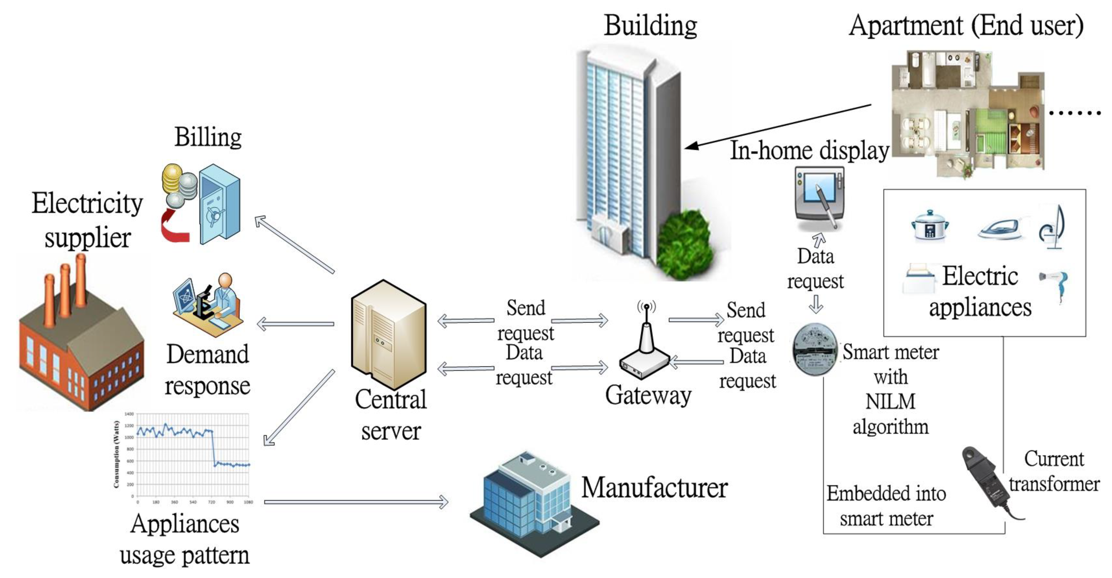
Figure 2.
Flow chart of research methodology. AI, artificial intelligence; GA-SVM, generic algorithm support vector machine.
Figure 2.
Flow chart of research methodology. AI, artificial intelligence; GA-SVM, generic algorithm support vector machine.

Figure 3.
Flow chart for the operation of generic algorithm support vector machine multiple kernel learning (GA-SVM-MKL) classifier for NILM.
Figure 3.
Flow chart for the operation of generic algorithm support vector machine multiple kernel learning (GA-SVM-MKL) classifier for NILM.
Figure 4.
Measurement set up for capturing voltage and current waveforms of electric appliances. CRO, cathode ray oscilloscope.
Figure 4.
Measurement set up for capturing voltage and current waveforms of electric appliances. CRO, cathode ray oscilloscope.

Figure 5.
Flow chart of the optimal design of the classifier using GA-SVM-MKL.
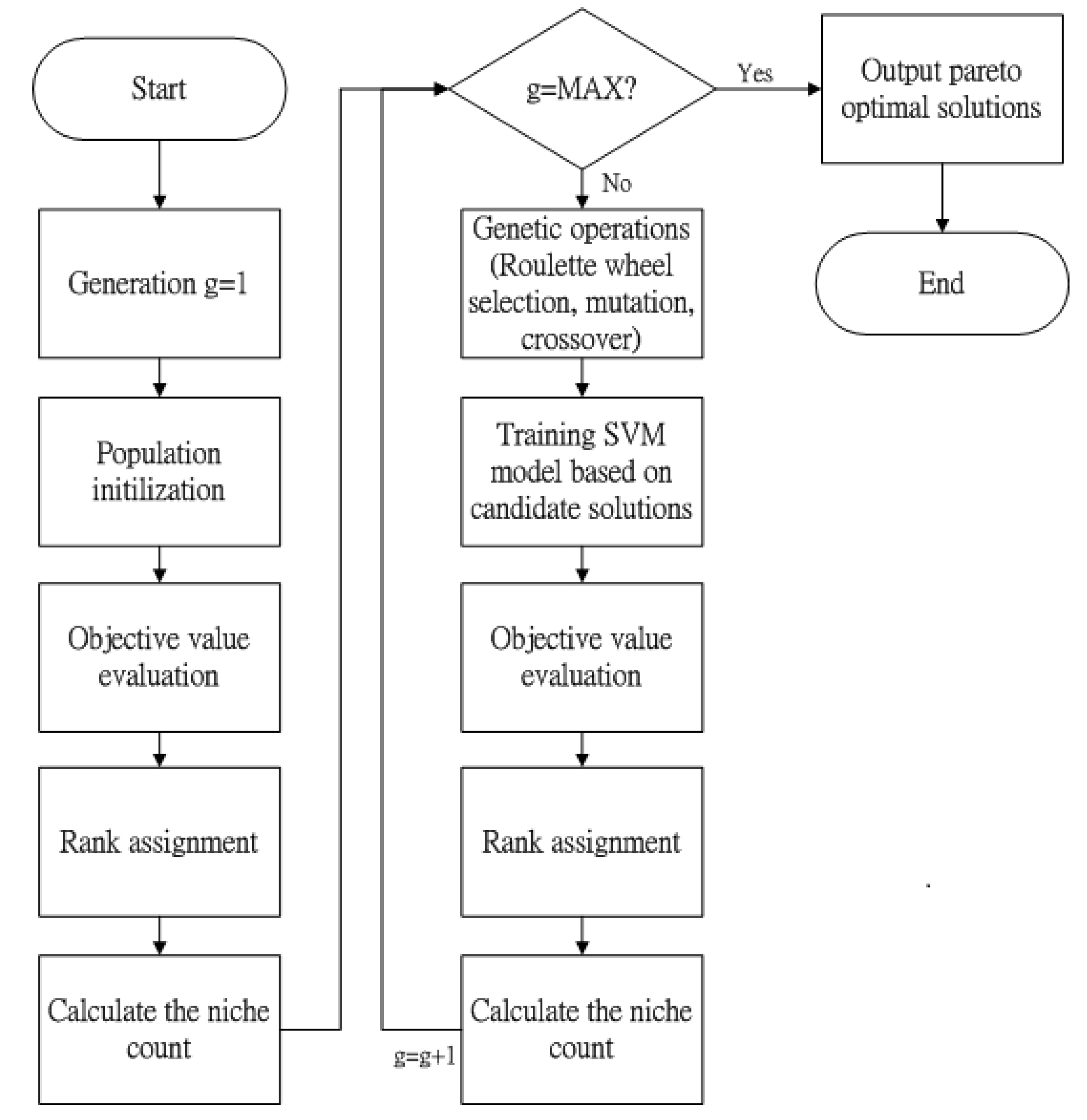
Table 1.
List of electric appliances that have been analyzed.
| Type of Activity | Electric Appliance | Modes | No. of Brands | Maximum No. of Appliances at One Time | Type of Activity | Electric Appliance | Modes | No. of Brands | Maximum No. of Appliances at One Time |
|---|---|---|---|---|---|---|---|---|---|
| Cooking | Electric stove | 2 | 3 | 2 | Lighting | Fluorescent light | 1 | 2 | 3 |
| microwave oven | 3 | 2 | 1 | Light bulb | 1 | 2 | 3 | ||
| cooker | 3 | 2 | 1 | LED tube | 1 | 3 | 3 | ||
| Home living | Ironbrush | 4 | 2 | 1 | LED light bulb | 1 | 2 | 3 | |
| Vacuum cleaner | 1 | 2 | 1 | Computing | Notebook | 1 | 6 | 3 | |
| Fan | 3 | 3 | 2 | desktop | 1 | 3 | 3 | ||
| Hair dryer | 2 | 3 | 2 | All in one printer and scanner | 1 | 2 | 1 | ||
| Electric heater | 2 | 2 | 1 | Mobile charger | 1 | 5 | 3 | ||
| Renovation | Electric drill | 1 | 2 | 1 | Audio and video | Radio | 1 | 2 | 1 |
| Electric sander | 1 | 2 | 1 | Television | 1 | 2 | 1 |
Table 2.
Comparisons between Proposed and Traditional SVM Classifier.
| Method | Se (%) | Sp (%) | OA (%) |
|---|---|---|---|
| GA-SVM-MKL | 92.1 | 91.5 | 91.8 |
| SVM using k1 | 71.6 | 72.2 | 71.9 |
| SVM using k2 | 72.3 | 72.8 | 72.6 |
| SVM using k3 | 73.5 | 74.2 | 73.9 |
| SVM using k4 | 75.9 | 75.3 | 75.6 |
| SVM using k5 | 74.9 | 75.1 | 75 |
Table 3.
Performance evaluation of assignment a class label for different modes in electric appliances.
Table 3.
Performance evaluation of assignment a class label for different modes in electric appliances.
| Scenario (S1 to S4) | Se (%) | Sp (%) | OA (%) |
|---|---|---|---|
| S1: 20 appliances (Different modes, same class) | 92.1 | 91.5 | 91.8 |
| S2: 32 appliances (Different modes, different classes) | 79.6 | 80.0 | 79.8 |
| S3: 32 appliances (only cooking related combinations) | 77.4 | 77.1 | 77.3 |
| S4: 32 appliances (only home living related combinations) | 75.3 | 76.6 | 76.0 |
Table 4.
Various Modes in GA-SVM-MKL classifier.
| Activity | Mode of Classifier | ||||
|---|---|---|---|---|---|
| Mode 1 | Mode 2 | Mode 3 | Mode 4 | Mode 5 | |
| Lighting | ✓ | ✓ | ✓ | ✓ | X |
| Cooking | ✓ | ✓ | X | X | X |
| Home living | ✓ | ✓ | ✓ | ✓ | X |
| Computing | ✓ | ✓ | ✓ | ✓ | X |
| Renovating | ✓ | X | ✓ | X | ✓ |
| Audio and video | ✓ | ✓ | ✓ | ✓ | X |
Table 5.
Performance Evaluation of GA-SVM-MKL classifier in each tunable modes (TM).
| Se | Sp and OA (%) of GA-SVM-MKL Classifier | |||||||||
|---|---|---|---|---|---|---|---|---|---|
| TM 1 | TM 2 | TM 3 | TM 4 | TM 5 | |||||
| Se | Sp | Se | Sp | Se | Sp | Se | Sp | Se | Sp |
| 92.1 | 91.5 | 93.8 | 94.3 | 94.6 | 94.1 | 96.6 | 96.1 | 98.4 | 98.8 |
| OA | 91.8 | OA | 94.1 | OA | 94.4 | OA | 96.4 | OA | 98.6 |
Table 6.
Performance comparisons between GA-SVM-MKL and related works.
| Work | Features | Dataset | Cross-Validation | Detection Interval | OA |
|---|---|---|---|---|---|
| Decision tree and wavelet transform [14] | approximation level and detail level | Four electric appliances—battery charger, compact fluorescent lamp, personal computer and incandescent light bulb (total 864 samples) | No | 0.0167 s (60 Hz) | 96.65% |
| Decision tree method [15] | the first increasing edge at the start of the event and the last decreasing edge at the end of the event | Ten Activities—cooking, washing, laundering, cleaning, watching TV, listening to radio, games, computing, hobbies and socializing (unknown sample size) | N/A | 8 s | 59% |
| Graph signal processing [16] | Active power edges | Nine electric appliances—416 microwave oven, 311 washer dryer, 61 oven, 330 lighting, 2228 refrigerator, 264 dishwasher, 138 stove, 62 heater and 54 air conditioner | No | 1 min | 77.2% |
| Factorial Hidden Markov Model [17] | Factorial main factors | Five electric appliances—90 microwave oven, 121 electric stove, 883 refrigerator, 58 dishwasher and 189 lighting | N/A | 1 min | 70.84% |
| Hidden Markov model [18] | log-odds score | Four electric appliances—2228 refrigerator, 416 microwave oven, 311 washing machine and 264 dishwasher | 50-fold | 1 min | N/A |
| k-nearest neighbor and artificial neural network [19] | maximum, average and root mean square of the current wave in transient stage | Four electric appliances—27 Fan, 30 Fluorescent light, 19 radio and 18 microwave oven | No | 0.02 s (50 Hz) | 97.87% |
| Clustering [20] | real power, reactive power, apparent power and voltage features | Seven electric appliances—800 oven, 56 refrigerator, 452 dishwasher, 65 lighting, 154 washer, 443 microwave oven, 236 dryer | No | 1 min | 77.6% |
| Cepstrum-smoothing [21] | Frequency and amplitude of the dominant peaks in the smoothed cepstrum | Six electric appliances—television, computer, monitor, refrigerator, washer and vacuum cleaner (unknown sample size) | N/A | 0.5 s | 96.37% |
| Proposed GA-SVM-MKL | Imax, Irms, Iavg, Pact, Papp, Prea and PF | 20 electric appliances—Fluorescent light, light bulb, LED tube, LED light bulb, electric stove, microwave oven, cooker, ironbrush, vacuum cleaner, fan, hair dryer, electric heater, notebook, desktop, all in one printer and scanner, mobile charger, electric drill, electric sander, radio and television (each of 1500 samples) | 10-fold | 0.02 s (50 Hz) | 91.8%, 94.1%, 94.4%, 96.4%, 98.6% for TM1 to TM5 |
© 2018 by the authors. Licensee MDPI, Basel, Switzerland. This article is an open access article distributed under the terms and conditions of the Creative Commons Attribution (CC BY) license (http://creativecommons.org/licenses/by/4.0/).
Share and Cite
MDPI and ACS Style
Chui, K.T.; Lytras, M.D.; Visvizi, A. Energy Sustainability in Smart Cities: Artificial Intelligence, Smart Monitoring, and Optimization of Energy Consumption. Energies 2018, 11, 2869. https://doi.org/10.3390/en11112869
AMA Style
Chui KT, Lytras MD, Visvizi A. Energy Sustainability in Smart Cities: Artificial Intelligence, Smart Monitoring, and Optimization of Energy Consumption. Energies. 2018; 11(11):2869. https://doi.org/10.3390/en11112869
Chicago/Turabian StyleChui, Kwok Tai, Miltiadis D. Lytras, and Anna Visvizi. 2018. "Energy Sustainability in Smart Cities: Artificial Intelligence, Smart Monitoring, and Optimization of Energy Consumption" Energies 11, no. 11: 2869. https://doi.org/10.3390/en11112869
Note that from the first issue of 2016, this journal uses article numbers instead of page numbers. See further details here.