Generalized Method of Moments Estimation of Realized Stochastic Volatility Model

Abstract

The purpose of this paper is to study the generalized method of moments (GMM) estimation procedures of the realized stochastic volatility model; we give the moment conditions for this model and then obtain the estimation of parameters. Then, we apply these moment conditions to the realized stochastic volatility model to improve the volatility prediction effect. This paper selects the Shanghai Composite Index (SSE) as the original data of model research and completes the volatility prediction under a realized stochastic volatility model. Markov chain Monte Carlo (MCMC) estimation and quasi-maximum likelihood (QML) estimation are applied to the parameter estimation of the realized stochastic volatility model to compare with the GMM method. And the volatility prediction accuracy of these three different methods is compared. The results of empirical research show that the effect of model prediction using the parameters obtained by the GMM method is close to that of the MCMC method, and the effect is obviously better than that of the quasi-maximum likelihood estimation method.

1. Introduction

Stock markets are not only one of the most important economic and financial markets in each country today, but their immaturity and institutional weaknesses can lead to serious divergences between their development and macroeconomic developments, mainly referring to the high volatility of stock prices, which makes asset pricing and effective portfolios subject to a lot of uncertainty. Therefore, the study of stock market volatility and more accurate estimation and prediction of stock market fluctuations play an important role and significance in reducing stock market risks, maintaining the safe and stable development of the stock market and ensuring the healthy and stable operation of the macro economy; refer to Brooks and Persand (2003); Giot and Laurent (2004). With the rapid advancement of computer technology, accessing high-frequency financial data has become easier. Using high-frequency data, we can estimate realized volatility; refer to Andersen et al. (2003); Barndorff-Nielsen and Shephard (2003a, 2003b); Jacod et al. (2009), etc. By incorporating high-frequency financial data, it provides a more accurate measure of market volatility compared to traditional methods.

The original stochastic volatility (SV) model was proposed by Taylor (1986) and others. Taylor (1986) proposed a discrete-time SV model, White (1984) proposed a continuous-time SV model, and Harvey and Shephard (1996) discussed an asymmetric SV model with leverage effects between the return process and the stochastic volatility process in the SV model using the quasi-maximum likelihood estimation method. Han et al. (2016) described an asymmetric stochastic volatility model using Gaussian regression with parameter estimation using the sequential Monte Carlo method.

The inclusion of unobservable potential random variables in the SV model makes the implementation of parameter estimation methods for the SV model very complicated. Commonly used parameter estimation methods include the generalized method of moments (Taylor (1986); Andersen and Sørensen (1996)), quasi-maximum likelihood method (Harvey et al. (1994); Harvey and Shephard (1996)), Markov chain Monte Carlo method (Kim et al. (1998); Yu (2005); Takahashi et al. (2021)), Bayesian method (Jacquier et al. (2002, 2004); Liu (2021); Bormetti et al. (2020)), and efficient method of moments (Andersen et al. (1999); Bansal et al. (1995); Gallant and Tauchen (1996)).

Financial return volatility is defined as the standard deviation of returns and plays a central role in modern finance. Realized volatility is the sum of the squares of intra-day returns over an interval and is used by modern financial economists and econometricians as a measure of true volatility. Andersen and Bollerslev (1997) thought the realized volatility proposed would provide a stable estimate of the potential volatility under the assumption of an ideal market. However, in real markets, measuring daily realized volatility based on high-frequency return data raises problems related to the presence of microstructure noise of the trading market. There are many noise-robust approaches of realized volatility (see Zhang et al. (2005); Barndorff-Nielsen et al. (2008); Xiu (2010); Jacod et al. (2009) and references therein). We apply the pre-averaging method (Jacod et al. (2009)) to estimate the realized volatility using high-frequency data.

Realized volatility reveals some important information of volatility; combining realized volatility into a traditional volatility model can improve the forecasting effect. Hansen et al. (2012, 2014) incorporated realized volatility with a generalized autoregressive conditional heteroscedasticity model. Takahashi et al. (2009) explores a stochastic volatility model with realized volatility, selecting the new sampling method and using the Markov chain Monte Carlo method for parameter estimation. Chaussé and Xu (2018) used four generalized methods of moments for the generalized asymmetric stochastic volatility with a realized volatility model (GASV-RV) and concluded that the efficiency of the GMM was improved by automatic moment selection through the principal component GMM and regularized GMM procedures.

This paper uses realized volatility constructed from high-frequency data and adds it to the stochastic volatility model to improve the prediction of volatility; the new model is called the realized stochastic volatility model. We employ the GMM method to estimate the parameters of the realized stochastic volatility model. The paper presents the theoretical moment conditions of the realized stochastic volatility model; the research contribution is providing the moment conditions for realized volatility. Furthermore, we explore the accuracy of GMM by comparing it with other two methods, MCMC and QML, which are utilized for parameter estimation in the realized stochastic volatility model.

We introduce the realized stochastic volatility model in Section 2. Estimation of realized volatility is given in Section 3. Three parameter estimation methods are introduced in Section 4. Section 5 provides an empirical illustration and demonstrates the effectiveness of three different parameter estimation methods. Section 6 contains the conclusion.

2. Realized Stochastic Volatility Model

Considering the realized volatility measure in the traditional SV model, the realized stochastic volatility (RSV) model is constructed by Takahashi et al. (2009). Compared with the traditional SV model, the RSV model contains more intra-day information, which is helpful to improve the prediction performance of the model inside and outside the sample. The specific RSV model is expressed as follows:

$$y_t=\exp (h_t/2){ϵ}_t,{ϵ}_t\sim N(0,1),$$

(1)

$$z_t=\xi +h_t+u_t,u_t\sim N(0,{\sigma }_u^2),$$

(2)

$$h_{t+1}=\mu +\varphi (h_t-\mu )+{\eta }_t,{\eta }_t\sim N(0,{\sigma }_{\eta }^2),$$

(3)

$$h_1=\mu +{ϵ}_0,{ϵ}_0\sim N(0,\frac{{\sigma }_{\eta }^2}{1-{\varphi }^2}).$$

(4)

In the yield equation $y_t$, the volatility ${\sigma }_t=\exp (h_t/2)$ plays the role of a constant scale factor, and $h_t$ is the unobserved potential volatility. To ensure the strict stationarity and iterative nature of the stochastic process, the persistence parameter $\left|\varphi \right|<1$ is assumed in the logarithmic volatility equation $h_t$ and set $h_1$. ${ϵ}_t$ and ${\eta }_t$ are random error terms. Theoretically, when the error term ${\eta }_t$ obeys the standard normal distribution, $h_t$ is a stationary process of AR(1), following the normal distribution with the mean value of $\mu$ and the variance of ${\sigma }_{\eta }^2/(1-{\varphi }^2)$. The RSV model is composed by adding a metric Equation (2) to the rate of return equation and the state equation of the SV model. Where $z_t$ is the realized volatility at time t, the pre-averaging method can be chosen for the estimation of realized volatility, ${\sigma }_u^2$ is the variance of the new interest $u_t$, the smaller the ${\sigma }_u^2$, the better the fit of the model, $\xi$ is the bias correction term of the realized volatility measure. We use the pre-averaging method to estimate the realized volatility, because this method can handle the microstructure noise problem when using high-frequency data.

3. Realized Volatility

The term volatility comes from mathematical statistics, and it is an indicator used to measure the level of price volatility and reflects the extent to which prices deviate from their average value. Realized volatility is an estimation of integrated volatility. When using high-frequency data, the traditional realized volatility estimator will be dominated by noise and will not have convergence to the integrated volatility. In this work, the pre-averaging method is used to calculate the realized volatility, which is proposed by Jacod et al. (2009). This method can reduce the effect of microstructure noise, and the estimator is a consistent estimator for the integrated volatility. Precisely, the latent price is $X_i^n=X_{i{\Delta }_n}$, ${\Delta }_n=1/n$, the noise price is ${ϵ}_i^n={ϵ}_{i{\Delta }_n}$, and the observed contaminated data are represented by $Z_i^n=Z_{i{\Delta }_n}$,

$$Z_i^n=X_i^n+{ϵ}_i^n.$$

(5)

We choose a sequence $k_n$ and a number $\theta$ that satisfies $k_n\sqrt{{\Delta }_n}=\theta +o({\Delta }_n^{1/4})$. $g(x)$ be a function defined in $[0, 1]$ which satisfies g is continuous, piecewise $C^1$ with a piecewise Lipschitz derivative $g^{\prime }$. Denote $g_j^n:=g(\frac{j}{k_n})$ for $j=0,1,\cdots ,k_n$, then we define the pre-averaged increments: ${\overline{Z}}_i^n={\displaystyle \sum _{j=1}^{k_n-1}}{g}_j^n{\Delta }_{i+j}^{n}Z,{\Delta }_i^{n}Z=Z_i^n-Z_{i-1}^n,i=0,1,\cdots ,n-k_n+1$.

The pre-averaged estimator is

$${\widehat{C}}_t^n=\frac{\sqrt{{\Delta }_n}}{\theta {\psi }_2}{\displaystyle \sum _{i=0}^{[t/{\Delta }_n]-k_n+1}}{({\overline{Z}}_i^n)}^2-\frac{{\psi }_1{\Delta }_n}{2{\theta }^2{\psi }_2}{\displaystyle \sum _{i=1}^{[t/{\Delta }_n]}}{({\Delta }_i^{n}Z)}^2.$$

(6)

In this case, we choose

$$g(x)=x\wedge (1-x),{\psi }_1=1,{\psi }_2=\frac{1}{12},\theta =\frac{1}{3}.$$

(7)

When using Equation (2), we employ the value of ${\widehat{C}}_t^n$ to replace $z_t$, which represents the realized volatility.

4. Parameter Estimation Methods

4.1. GMM Method Based on RSV Model

The GMM method was first proposed by Hansen (1982). It is a generic method for estimation parameters in semiparametric models. The method requires a certain number of moment conditions that are specified for the model. In this work, we refer to the method used in Jacquier et al. (2002) to construct moment conditions for the rate of return and have the following theorem.

Theorem 1.

Given the RSV model given in Equations (1)–(3), for $0\le j\le 10$, the first four order moments and the cross-moment expressions for $y_t$ and $y_{t+j}$ are

$$E|y_t|=\sqrt{2/\pi }E(h_t),$$

(8)

$$E(y_t^2)=E(h_t^2),$$

(9)

$$E|y_t^3|=2\sqrt{2/\pi }E(h_t^3),$$

(10)

$$E(y_t^4)=3E(h_t^4),$$

(11)

$$E|y_t{y}_{t+j}|=(2/\pi )E(h_t{h}_{t+j}),j=1,2,\dots ,10,$$

(12)

$$E(y_t^2{y}_{t+j}^2)=E(h_t^2{h}_{t+j}^2),j=1,2,\dots ,10,$$

(13)

where, $E(h_t^r)=exp(\frac{r\mu }{2}+\frac{r^2{\sigma }^2}{8})$, $E(h_t^r{h}_{t+j}^s)=E(h_t^r)E(h_t^s)exp(\frac{rs{\varphi }^j{\sigma }^2}{4})$, ${\sigma }^2=\frac{{\sigma }_{\eta }}{1-{\varphi }^2}$.

Referring to the proof of the moment condition in Chaussé and Xu (2018), this paper gives the moment condition that the RSV model has the realized volatility term, which is proved as follows.

Proposition 1.

Given the RSV model specified in Equations (1)–(3), the first two order moments and the cross-moment expressions for $z_t$ and $z_{t+j}(0\le j\le 10)$ are

$$E(z_t)=\xi +\frac{\mu }{1-\varphi },$$

(14)

$$\begin{array}{cc}\hfill E({z_t}^2)& \hfill ={\xi }^2+\frac{{\mu }^2}{{(1-\varphi )}^2}+\frac{{\sigma }_{\eta }^2}{1-{\varphi }^2}+{\sigma }_u^2+2\frac{\xi \mu }{1-\varphi },\hfill \end{array}$$

(15)

$$\begin{array}{ccc}\hfill E(z_t{z}_{t+j})& \hfill =\hfill & {\xi }^2+2\frac{\xi \mu }{1-\varphi }+\frac{{\mu }^2}{1-\varphi }{\displaystyle \sum _{i=1}^j}{\varphi }^{i-1}+{\varphi }^j(\frac{{\sigma }_{\eta }^2}{1-{\varphi }^2}+\frac{{\mu }^2}{{(1-\varphi )}^2}),\hfill \\ \hfill j& \hfill =\hfill & 1,2,\dots ,10.\hfill \end{array}$$

(16)

Proof of Proposition 1.

Given $z_t$ and $h_t$ specified in (2),

$$E(z_t)=\xi +E(h_t)=\xi +\frac{\mu }{1-\varphi },$$

(17)

$$\begin{array}{cc}\hfill E({z_t}^2)& \hfill ={\xi }^2+E({h_t}^2)+E({u_t}^2)+2\frac{\xi \mu }{1-\varphi }+2E(h_t{u}_t)\hfill \\ \hfill & \hfill ={\xi }^2+\frac{{\mu }^2}{{(1-\varphi )}^2}+\frac{{\sigma }_{\eta }^2}{1-{\varphi }^2}+{\sigma }_u^2+2\frac{\xi \mu }{1-\varphi },\hfill \end{array}$$

(18)

$$\begin{array}{ccc}\hfill E(z_t{z}_{t+j})& \hfill =\hfill & {\xi }^2+2\frac{\xi \mu }{1-\varphi }+E[h_t(\mu {\displaystyle \sum _{i=1}^j}{\varphi }^{j-1}+{\varphi }^j{h}_t+{\displaystyle \sum _{i=1}^j}{\varphi }^{j-i}{\eta }_{t+i-1})]\hfill \\ \hfill & \hfill =\hfill & {\xi }^2+2\frac{\xi \mu }{1-\varphi }+\frac{{\mu }^2}{1-\varphi }{\displaystyle \sum _{i=1}^j}{\varphi }^{i-1}+{\varphi }^j(\frac{{\sigma }_{\eta }^2}{1-{\varphi }^2}+\frac{{\mu }^2}{{(1-\varphi )}^2}),\hfill \\ \hfill j& \hfill =\hfill & 1,2,\dots ,10.\hfill \end{array}$$

(19)

□

Let ${\psi }_t$ be a $q\times 1$ vector with typical element $(y_t^n{y}_{t+j}^m)$, $(z_t^n{z}_{t+j}^m)$ for some $m,j,$ and $n\in (0,1,2,3,\dots )$, and let $\psi ({\theta }_0)=E({\psi }_t({\theta }_0))$ be the theoretical moments of the RSV model. Let $g_t(\theta )=[{\psi }_t-\psi (\theta )]$; then, the GMM estimator $\widehat{\theta }$ of the true vector of coefficients ${\theta }_0$ is based on the following moment conditions:

$$E[g_t({\theta }_0)]=0,$$

(20)

and is the solution to:

$$\underset{\theta \in \mathrm{\Theta }}{\mathrm{argmin}}\overline{g}{(\theta )}^{\prime }{\widehat{\mathrm{\Omega }}}^{-1}\overline{g}(\theta ).$$

(21)

where $\mathrm{\Theta }$ is the admissible parameter space implied by the model, $\overline{g}(\theta )=[{\sum }_{t=1}^T\frac{{\psi }_t}{T}-\psi (\theta )]$ and $\widehat{\mathrm{\Omega }}$ is a consistent estimate of the auto-correlation matrix of $\sqrt{n}\overline{g}({\theta }_0)$.

Therefore, the estimator defined by Equation (21) is a one-step GMM with the estimate of the auto-correlation consistent (HAC) matrix given by:

$$\widehat{\mathrm{\Omega }}={\displaystyle \sum _{i=-T+1}^{T-1}}{\omega }_h(i){\widehat{\mathrm{\Gamma }}}_i,$$

(22)

where ${\omega }_h(i)$ is a kernel, and h is the bandwidth, which can be chosen using the procedures proposed by Newey and West (1986) and Andrews (1991),

$${\widehat{\mathrm{\Gamma }}}_i=\frac{1}{T}\sum _t({\psi }_t-\overline{\psi }){({\psi }_{t+i}-\overline{\psi })}^{\prime }.$$

(23)

In order to improve the properties of the two-step GMM, Hansen (1982) suggested two other methods. The first one is the iterative version of the two-step GMM and can be computed as follows:

• Compute ${\theta }^{(0)}={\mathrm{argmin}}_{\theta }\overline{g}{(\theta )}^{\prime }\overline{g}(\theta )$;
• Compute the HAC matix $\widehat{\mathrm{\Omega }}({\theta }^{(0)})$;
• Compute the ${\theta }^{(1)}={\mathrm{argmin}}_{\theta }\overline{g}{(\theta )}^{\prime }{[\widehat{\mathrm{\Omega }}({\theta }^{(0)})]}^{(-1)}\widehat{g}(\theta )$;
• If $\left|\right|{\theta }^{(0)}-{\theta }^{(1)}\left|\right|<tol$ stops, else ${\theta }^{(0)}={\theta }^{(1)}$ and go to step 2;
• Define the two-step GMM estimator $\widehat{\theta }$ as ${\theta }^{(1)}$;

where $tol$ can be set as small as we want to increase the precision.

4.2. MCMC Method Based on RSV Model

In this paper, the MCMC method is used to estimate the parameters of the RSV model as a comparison with the GMM method. In the estimation, the prior distribution of the parameters is estimated and the conditional distribution of the combined sample information is given first, and then, the posterior distribution of the parameters to be estimated is calculated and the parameters of the models can be estimated for specific problems using the WinBUGS 1.4.3 software package.

Consider the RSV model described in (1)–(4). When given $h=(h_1,\dots ,h_T)$, referring to Takahashi et al. (2009), we can compute the conditional likelihood of the RSV model as:

$$\begin{array}{c}\hfill f(y_1,z_1,\dots ,y_T,z_T|\overline{\theta },h)={\displaystyle \prod _{t=1}^T}\frac{1}{\sqrt{2\pi }\exp (h_t/2)}\exp \{-\frac{y_t^2}{2\exp (h_t)}\}\\ \hfill \times \frac{1}{\sqrt{2\pi }{\sigma }_u}\exp \{-\frac{{(z_t-\xi -h_t)}^2}{2{\sigma }_u^2}\},\end{array}$$

(24)

where $\overline{\theta }=(\xi ,{\sigma }_u^2,\mu ,\varphi ,{\sigma }_{\eta }^2)$ denotes the parameters. Therefore, we use a Bayesian approach to estimate the posterior distribution of the parameters of the RSV model, considering h as an additional latent variable. In this setup, the most important thing is how to sample h efficiently. Therefore, we first describe the sampling algorithm for h.

When selecting the parameter’s prior distributions, we refer to the setting in Yu (2005), and we set priors as: $\xi \sim N(0,27)$, ${\sigma }_u^2\sim IG(2.5,0.027)$, $\mu \sim N(0,25)$, $\frac{1+\varphi }{2}\sim Beta(20,1.5)$, ${\sigma }_u^2\sim IG(2.5,0.025)$. Then, denoting $Y=(y_1,\dots ,y_T)$ and $Z=(z_1,\dots ,z_T)$, the posterior density for $\overline{\theta }=(\xi ,{\sigma }_u^2,\mu ,\varphi ,{\sigma }_{\eta }^2)$ and h becomes

$$\begin{array}{cc}\hfill f(\overline{\theta },h|Y,Z)& \propto \exp [-\frac{1}{2}{\displaystyle \sum _{t=1}^T}{y}_t^2\exp (-h_t)]{({\sigma }_u^2)}^{-T/2}\exp \{-\frac{1}{{\sigma }_u^2}{\displaystyle \sum _{t=1}^T}{(z_t-\xi -h_t)}^2\}\hfill \\ \hfill & \times \sqrt{1-{\varphi }^2}{({\sigma }_u^2)}^{-T/2}\exp \{-\frac{1}{2{\sigma }_{\eta }^2}(1-{\varphi }^2){(h_1-\mu )}^2\hfill \\ \hfill & -\frac{1}{2{\sigma }_{\eta }^2}{\displaystyle \sum _{t=1}^{T-1}}{(h_{t+1}-(1-\varphi )\mu -\varphi h_t)}^2\}\hfill \\ \hfill & \times \exp \{-\frac{{(\xi )}^2}{54}\}{({\sigma }_u^2)}^{-3.5}\exp (-\frac{0.027}{{\sigma }_u^2})\exp \{-\frac{{(\mu )}^2}{50}\}\hfill \\ \hfill & \times {(\frac{1+\varphi }{2})}^{19}{(\frac{1-\varphi }{2})}^{0.5}{({\sigma }_{\eta }^2)}^{-3.5}\exp (-\frac{0.025}{{\sigma }_{\eta }^2}).\hfill \end{array}$$

(25)

To implement the Markov chain Monte Carlo simulation, we sample from the posterior distribution as follows:

• Simulate h from $f(h|\mu ,\varphi ,{\sigma }_{\eta }^2,Z,Y)$.
• Simulate $\xi$ from $f(\xi |h,{\sigma }_u^2,Z)$.
• Simulate ${\sigma }_u^2$ from $f({\sigma }_u^2|h,\xi ,Z)$.
• Simulate $\mu$ from $f(\mu |h,\varphi ,{\sigma }_{\eta }^2)$.
• Simulate ${\sigma }_{\eta }^2$ from $f({\sigma }_{\eta }^2|h,\mu ,\varphi )$.
• Simulate $\varphi$ from $f(\varphi |h,\mu ,{\sigma }_{\eta }^2)$.

4.3. QML Method Based on RSV Model

In this work, QML estimation is also performed for the RSV model. Due to the nonlinear relationship between the daily returns and the log of latent volatility in the Equations (1)–(3), we cannot compute the likelihood of these models by the Kalman filter. But given the parameter vector of the RSV model is $\overline{\theta }=(\mu ,\varphi ,{{\sigma }_{\eta }}^2,\xi ,{{\sigma }_u}^2)$, the log latent volatility is $h=(h_1,\dots ,h_T)$, and by referencing Takahashi et al. (2009), we can compute the conditional likelihood of the RSV model as:

$$\begin{array}{c}\hfill f(y_1,z_1,\dots ,y_T,z_T|\overline{\theta },h)={\displaystyle \prod _{t=1}^T}\frac{1}{\sqrt{2\pi }\exp (h_t/2)}\exp \{-\frac{y_t^2}{2\exp (h_t)}\}\\ \hfill \times \frac{1}{\sqrt{2\pi }{\sigma }_u}\exp \{-\frac{{(z_t-\xi -h_t)}^2}{2{\sigma }_u^2}\}.\end{array}$$

(26)

Then, the RSV model log-likelihood function can be written as:

$$\log \widehat{L}(\overline{\theta })=\log f(y_1,z_1,\dots ,y_T,z_T|\overline{\theta },h)={\displaystyle \sum _{t=1}^T}\log f(y_t,z_t|\overline{\theta },h).$$

(27)

The log-likelihood estimation obtained from the above equation is a continuous function of the RSV model parameter $\overline{\theta }$. Then, the parameter $\overline{\theta }$ of this model can be estimated by virtue of the classical proposed maximum likelihood estimation method obtained as follows.

$$\widehat{\theta }=\underset{\mathrm{\Theta }}{\mathrm{argmax}}\log \widehat{L}(\overline{\theta }),$$

(28)

where $\mathrm{\Theta }$ is the admissible parameter space implied by the model.

5. Empirical Research

In this part, an empirical study will be conducted using the data of the Shanghai Stock Exchange (SSE) Composite Index from 4 January 2005 to 15 December 2022. The GMM method is used for estimating the parameters in the RSV model. The QML method and MCMC methods are also used in the RSV model for a comparative study.

5.1. Loss Functions

To measure different methods’ estimation and prediction performance, loss functions, also known as objective functions, are needed for measuring the errors between the actual volatility and predicted volatility. For regression data, the mean square error (MSE), root mean square error (RMSE), mean absolute error (MAE) and mean absolute percentage error (MAPE) are often used. The mean square error refers to the expected value of the square of the difference between the estimated value and the true value. The root mean square error is the arithmetic square root of the mean square error, which can directly observe the direct difference between the predicted value and the real value. The mean absolute error can better reflect the actual error between the predicted value and the actual value. The mean absolute percentage error is a measure of relative error, which uses the absolute value to avoid the positive error and negative error canceling each other. The relative error can be used to compare the prediction accuracy of various time-series models. The loss functions mentioned above are defined as follows:

$$\mathrm{MSE}=\frac{1}{T}{\displaystyle \sum _{t=1}^T}{(\widehat{h_t}-R{V}_t)}^2,$$

(29)

$$\mathrm{RMSE}=\sqrt{\frac{1}{T}{\displaystyle \sum _{t=1}^T}{(\widehat{h_t}-R{V}_t)}^2},$$

(30)

$$\mathrm{MAE}=\frac{1}{T}{\displaystyle \sum _{t=1}^T}|\widehat{h_t}-R{V}_t|,$$

(31)

$$\mathrm{MAPE}=\frac{1}{T}{\displaystyle \sum _{t=1}^T}|\frac{\widehat{h_t}-R{V}_t}{R{V}_t}|,$$

(32)

where $\widehat{h_t}$ is the predicted volatility at time t, T is the count number of the model forecast, and $R{V}_t$ is the realized volatility estimated by the pre-averaged estimator.

5.2. Data Selection and Processing

We used high-frequency data for the SSE Composite Index for the period from 4 January 2005 to 15 December 2022. The sample length is 4363, where the first 3963 trading days of data are selected for in-sample fitting and the last 400 trading days of data are selected for out-of-sample prediction. The frequency of our observed stock data is every five minutes. For a normal trading day, there are 48 observations. The data used in the empirical analysis are sourced from the Oxford-Man Institute of Quantitative Finance Realized Library and the Wind database. Prior to conducting the empirical analysis, certain processing steps are required for the return variable, $r_t$.

• The logarithm of the stock index closing price data for each stock market trading day is $\log (p_t)$, $t=1,\dots ,T$, forming a logarithmic price series $(\log (p_1),\dots ,\log (p_T))$;
• The logarithmic price series are differenced to obtain the return $r_t=\log (p_t)-\log (p_{t-1})$, $t=1,\dots ,T$ for the t-th trading day and then constitute the return sequence $(r_1,r_2,\dots ,r_T)$.

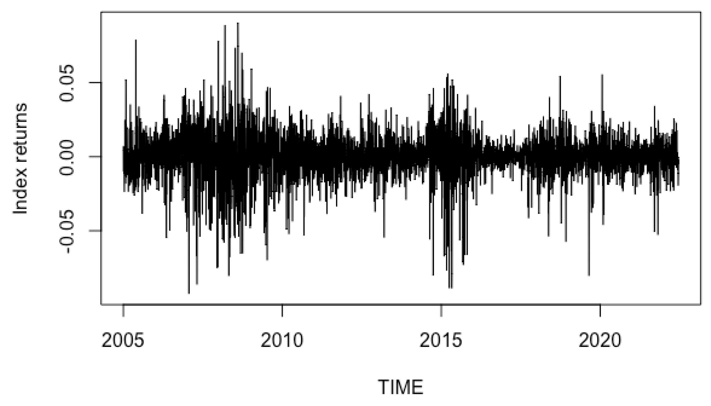
Figure 1 below is the index returns of SSE. We can see the irregular and aggregation of the SSE stock index return volatility. In the three phases 2007–2009, 2015–2016 and 2018–2020, the SSE composite index return volatility is large, and extreme values are more prominent. As we know, there are relatively large stock price fluctuations during these three periods since the financial crisis and economic market downturn.

5.3. Model Parameter Estimation

We use the daily return series of the SSE Composite Index to represent $y_t$ in Equation (1). In addition, we use the five-minute high-frequency return series of the SSE Composite Index to estimate the pre-averaged realized volatility in (6), and we use it as $z_t$ in Equation (2). The GMM method and QML method are used to estimate the parameters of the RSV model by R 4.1.3 language software. The MCMC method is used to estimate the parameters of the RSV model using WinBUGS software. WinBUGS’ basic principle is to sample from the complete conditional probability distribution through Gibbs sampling and the Metropolis algorithm, so as to generate a Markov chain, and finally estimate the model parameters through iteration. The obtained parameter estimation results are shown in

Table 1. Parameter estimation results for RSV model using different methods.

Method	$\mathit{\mu }$	$\mathit{\varphi }$	${\mathit{\sigma }}_{\mathit{\eta }}$	$\mathit{\xi }$	${\mathit{\sigma }}_{\mathit{u}}$
RSV-GMM	−0.2630743	0.9585373	0.1408710	1.1870245	0.9432676
	(0.14369)	(0.02479)	(0.08535)	(0.09746)	(0.00936)
RSV-MCMC	−0.1254	0.9473	0.2261	1.135	0.1211
	(0.15841)	(0.02923)	(0.05545)	(0.11521)	(0.00724)
RSV-QML	−0.22454762	0.9776021	0.1461197	0.7612748	0.9253961
	(0.149782)	(0.02637)	(0.01725)	(0.09839)	(0.00893)

Note: The number in parenthesis is the standard error.

. The advantage of introducing Gibbs sampling and MCMC is self-evident: that is, to avoid calculating a complete joint posterior probability publication with high-dimensional integral form and instead calculate the univariate conditional probability distribution of each estimated parameter.

Observing the persistence parameter $\varphi$, the parameter $\varphi$’s value of the RSV model of the SSE index is close to 1, indicating that the estimation results show that the time series of the SSE index has high persistent volatility characteristics. Next, observing the bias correction term $\xi$, the parameter $\xi$ of the RSV model is positive, indicating that the effect of market microstructure noise still persists.

The results of the parameters of the GMM method do not differ much from those of the QML method. The $\varphi$ values are still close to 1 and the persistence of volatility is still high.

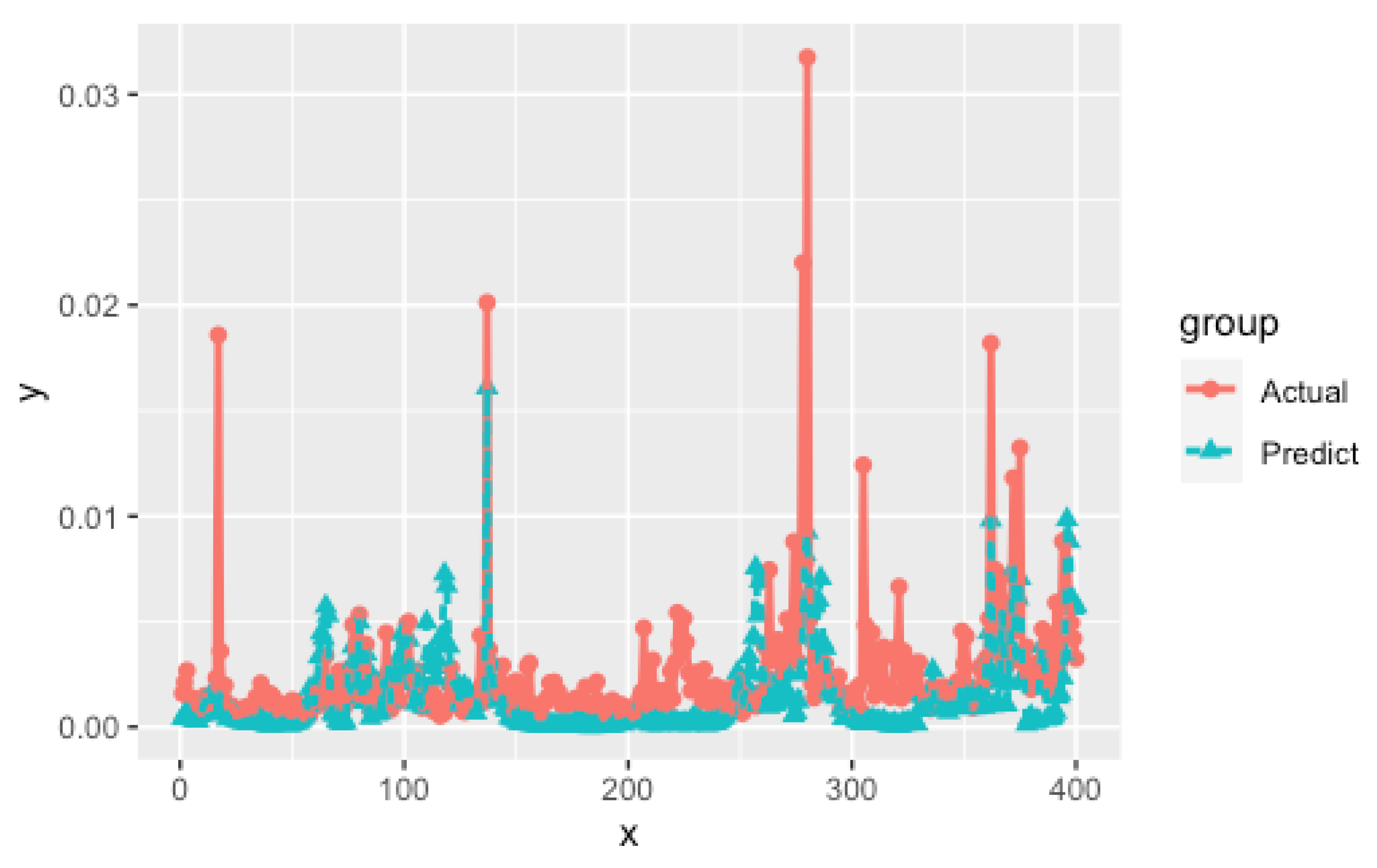
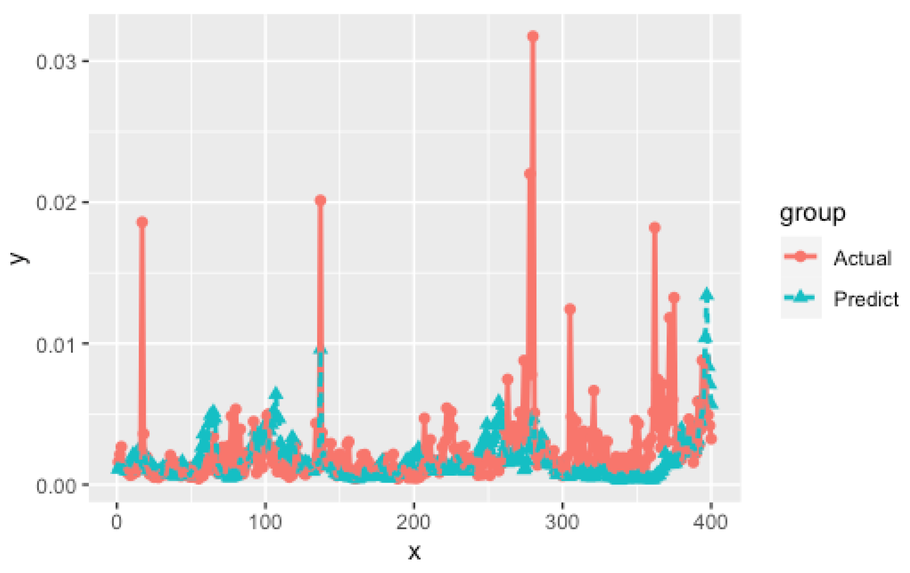
From Figure 2, Figure 3 and Figure 4, it is evident that the GMM method exhibits a notable ability to identify significant changes in volatility, particularly when volatility levels are high. The GMM method outperforms the MCMC, QML method in accurately predicting large volatility. The MCMC method performs well in forecasting, as it closely aligns the predicted volatility with the actual volatility. The predictive performance of the QML method in volatility estimation is satisfactory, yet it is not on par with the superior performance demonstrated by the GMM and MCMC approaches. The four loss functions are used to test the accuracy of the forecasting results.

The efficiency of three parameter estimation methods was investigated, and the results presented in

Table 2. Prediction errors of volatility forecasting using different methods for RSV model parameter estimation.

Model	MSE	RMSE	MAE	MAPE
RSV-GMM	0.02319271	0.1522915	0.04333079	0.0610987
RSV-MCMC	0.02319251	0.1522909	0.04308118	0.0610579
RSV-QML	0.03319375	0.1821915	0.05093191	0.0637402

demonstrate that, under the RSV model, using parameters obtained from the MCMC method yields the most effective predictions of volatility, followed by the GMM method, while the QML method performs relatively weaker. When the RSV model is used for volatility prediction, the error of predicting volatility using the parameters estimated by the GMM method is almost the same as that predicted by the MCMC method. It is worth mentioning that the MCMC method requires more computation time compared to the GMM method, yet the predictive performance remains comparable. This finding substantiates the effectiveness and utility of the GMM method of RSV model proposed in this study.

6. Conclusions

With the development of science and technology, people’s research in the field of stochastic volatility-type models parameter estimation is becoming more and more in-depth, and new parameter estimation methods are bound to appear. In this paper, GMM, MCMC and QML methods are used for realized stochastic volatility model parameter estimation, and we use these parameters and the realized stochastic volatility model to predict volatility. Empirical data are analyzed in this paper. We use the five-minute high-frequency return series of the SSE Composite Index, and we apply the pre-averaging method to estimate the realized volatility. The prediction results illustrate that the GMM method is very effective and the calculation speed is faster, while the MCMC method is also effective, and the QML method is less accurate.

Although the realized volatility is introduced on the basis of the random volatility model, this paper still assumes that the disturbance term obeys normal distribution. According to the research in recent years, it is shown that the model disturbance term obeys the generalized hyperbolic distribution, which may improve the prediction effect of the model. For the improved model, we can consider using the efficient generalized method of moments to estimate the unknown parameters.