Does the Hashrate Affect the Bitcoin Price?


1
Moscow School of Economics, Moscow State University, Leninskie Gory, 1, Building 61, Moscow 119992, Russia
2
Higher School of Economics, Moscow 109028, Russia
*
Author to whom correspondence should be addressed.
J. Risk Financial Manag. 2020, 13(11), 263; https://doi.org/10.3390/jrfm13110263
Submission received: 30 September 2020
/
Revised: 26 October 2020
/
Accepted: 27 October 2020
/
Published: 30 October 2020
(This article belongs to the Special Issue Financial Technology (Fintech) and Sustainable Financing)
Abstract
:This paper investigates the relationship between the bitcoin price and the hashrate by disentangling the effects of the energy efficiency of the bitcoin mining equipment, bitcoin halving, and of structural breaks on the price dynamics. For this purpose, we propose a methodology based on exponential smoothing to model the dynamics of the Bitcoin network energy efficiency. We consider either directly the hashrate or the bitcoin cost-of-production model (CPM) as a proxy for the hashrate, to take any nonlinearity into account. In the first examined subsample (01/08/2016–04/12/2017), the hashrate and the CPMs were never significant, while a significant cointegration relationship was found in the second subsample (11/12/2017–24/02/2020). The empirical evidence shows that it is better to consider the hashrate directly rather than its proxy represented by the CPM when modeling its relationship with the bitcoin price. Moreover, the causality is always unidirectional going from the bitcoin price to the hashrate (or its proxies), with lags ranging from one week up to six weeks later. These findings are consistent with a large literature in energy economics, which showed that oil and gas returns affect the purchase of the drilling rigs with a delay of up to three months, whereas the impact of changes in the rig count on oil and gas returns is limited or not significant.
JEL Classification:
C22; C32; C51; C53; E41; E42; E47; E51; G171. Introduction
There is a growing interest in bitcoin price dynamics both among the general public and in academia, see Burniske and Tatar (2018); Brummer (2019); Fantazzini (2019); Schar and Berentsen (2020). The price is not only important for purely speculative reasons but also for its role in the energy consumption of the Bitcoin network, and in affecting the future behavior of miners—agents who power the Bitcoin infrastructure by issuing new blocks containing the latest transactions.
There is a long-lived perception that the bitcoin price and the hashrate (i.e., the number of computations done by bitcoin miners) are connected, see for example Cointelegraph (2020). Some works in the financial literature went further and theorized that the movements of the hashrate are useful in predicting the bitcoin price (Hayes 2017, 2019; Aoyagi and Hattori 2019). At first glance, such a notion might seem wrong because producers are price-takers in competitive markets, and the amount of effort they put into the production of a good or service have no impact over the market price. However, this might not be the case for the bitcoin market. First, there are only a few mining pool operators, so that they can coordinate their actions in an attempt to control the market price. Second, the fact that bitcoin supply is inelastic and the mining business is very competitive might force miners to operate differently: they might be willing to cap their income by hedging their losses with the bitcoin futures introduced by the Chicago Mercantile Exchange and the CBOE in December 2017 (Chicago Mercantile Exchange 2017) as discussed in the cryptocurrency professional literature (see, for example, the several articles published on coindesk.com and cointelegraph.com)1. The exact economical behavior of miners is unknown and its modeling is beyond the scope of this paper. However, if we focus only on the influence of the hashrate on the bitcoin price dynamics, we can resort either to econometric models or to a general equilibrium model that omits the inner workings of miners’ decision-making but directly models the relationship between the hashrate and the price. Such an approach was first proposed by Hayes (2017), who put forward a methodology able to predict the bitcoin price using the total hashrate and the miners’ energy efficiency as inputs. Hayes (2019) showed that this model provided a surprisingly good fit and its equilibrium price was able to Granger-cause the bitcoin price. On the other hand, several works explained the dynamics of the bitcoin price using econometric models and various sets of explanatory variables, and they mostly found that the hashrate is not statistically significant and it does not help in predicting the bitcoin price, see Kjærland et al. (2018) and references therein.
These conflicting results drew our attention and became the main motivation for this work: we initially thought that this contradictory evidence could have been due to different sample periods (hence different price drivers at different times), but this is not the case: they largely intersect. A possible explanation could be that the hashrate is not useful in predicting the bitcoin price on its own, but it has a more complex relationship with it, as discussed by Hayes (2017).
In this paper, we examine the relationship between the hashrate (or the bitcoin cost-of-production price) and the market price, and we try to reconcile the previous contradictory findings by disentangling the effects of the energy efficiency of the bitcoin mining equipment, bitcoin halving, and of structural breaks on the price dynamics.
The first contribution of the paper is a methodology based on exponential smoothing to model the dynamics of the Bitcoin network energy efficiency as a whole. This type of smoothing naturally trails the data and it does not use future values: the data related to future mining equipment cannot be used to infer today’s performance to avoid any form of look-ahead bias. Moreover, this approach easily models the gradual replacement of old equipment with the new units.
The second contribution of the paper is a set of multivariate models to investigate the nature of the relationship between the bitcoin market price and the hashrate, both directly or through the proxy of production costs.
The third contribution of the paper is a robustness check to verify how our results change when computing the bitcoin cost-of-production using an electricity price no more fixed to a constant but equal to the daily data of the Nord pool system price, which is the unconstrained market-clearing reference price for the European Nordic region.
The paper is organized as follows: Section 2 briefly reviews the literature devoted to bitcoin and the cost-of-production model, while the methods proposed to investigate the relationship between the bitcoin market price and the hashrate are discussed in Section 3. The empirical results are reported in Section 4, while a robustness check is discussed in Section 5. Section 6 briefly concludes. A brief overview of Bitcoin’s operation is reported in the Appendix A.
2. Literature Review
One of the main approaches to model the bitcoin price behavior was introduced by Hayes (2017), and it is usually known as the “cost-of-production model” (CPM). The core of this approach is the attempt to derive the bitcoin cost of production for a given miner from the current state of the network, the energy prices, and the energy efficiency of the miner’s equipment. The CPM thus gives the break-even cost of mining, which any individual miner would use when trying to define whether he should be involved in mining bitcoin. Hayes (2017) generalized this approach for the whole network.
Hayes (2017) makes a few assumptions to estimate the main drivers of the bitcoin price. The first one is that the more computational power is employed by the Bitcoin network, the higher its value is. The second assumption simply states that all miners are rational, meaning that they are only willing to mine for bitcoin if they are looking to extract profit. This also implicitly means that any other cryptocurrency with no demand for it would have zero value and zero mining effort employed, and a rational miner would redirect its resources elsewhere. The third and final assumption is that the network difficulty can be used as a proxy of the aggregate mining power. Within the Bitcoin network, this assumption is directly supported by the algorithm governing it: difficulty always readjusts to ease off the effect of increased mining power or, in the opposite case, to make up for its decrease. Hayes (2017) builds a framework aimed at showing the connection between the computational power employed by a miner and its expected profit given the current network conditions. When a single miner estimates its baseline profitability, it first calculates the expected number of bitcoins produced per day:
where is block reward (bitcoin per block), is the difficulty (expressed in units of Giga-Hash/block), is the hashing power employed by a miner expressed in Giga-Hash/second, is the number of seconds in an hour, is a number of hours in a day and is a normalized probability of a single hash “solving” a block and is an attribute of the mining algorithm. These three constants can be fit into a single parameter , so the formula takes the following view:
The daily cost of mining can be expressed as follows,
where is the cost per day for a producer, is the price of a kilowatt-hour, and is the energy consumption efficiency of the miner’s hardware. Given the assumption of perfect competition so that the marginal cost of production and the marginal profit are equal, the equilibrium price takes the following form:
where we set GH/s as in Hayes (2017). The CPM offers a simple but effective framework for estimating the cost of production price. However, it simplifies the mining expenses by dismissing several other important factors, such as the capital and the operational expenses of the running mining operation. Another important drawback of this model emerges around the times of the bitcoin halving events, when the reward in bitcoins for finding new blocks is cut in half: unlike real-world miners, this model does not anticipate this change and therefore it produces unreliable results (this issue will be discussed later in this paper). Interestingly, Hayes (2019) found that the CPM Granger-causes the market price but not the other way around.
It is important to remark that the CPM proposed by Hayes (2017, 2019) requires a few inputs which cannot be directly observed or reliably approximated: one such input is the electricity cost, which is assumed by Hayes to be a constant equal to USD 0.135 per kWh—an average rate for electricity worldwide at the time of publishing those two papers. Of course, this is not always the case for miners: there are multiple reports of some miners having free energy (either as a form of subsidy or just by using it covertly), which are cited and discussed in Stoll et al. (2019). Another input is the parameter for the equipment’s energy efficiency: while it is possible to determine the best mining equipment available at a certain point in time, it is impossible to know the distribution of this equipment among miners and thus the average energy efficiency of the network. Moreover, there are ASIC models whose presence on the market is very limited, but the impact may be high, like—for example—the GMO miners (gmominer.z.com/en). Therefore, this situation makes it very difficult to assess the real picture of the total energy efficiency. The CPM relies heavily on the above-mentioned data (particularly the energy efficiency), so one has to be very careful when fixing these two parameters.
Kristoufek (2015) was among the first to highlight that the drivers behind the bitcoin price tend to vary over time due to the “dynamic nature of bitcoin and its rapid price fluctuations”. This idea was later developed and expanded by Kjærland et al. (2018), who used several major commodities and indices, different metrics from the Bitcoin network, and the Google Trends data as explanatory variables to find which factors affect the bitcoin price dynamics. Kjærland et al. (2018) transformed the original daily data into weekly averages to avoid potential issues related to autocorrelation. Moreover, they also deal with outliers in the data and structural breaks. The data sample was then divided into three smaller periods, and Autoregressive Distributed Lag (ARDL) and Generalized Autoregressive Conditional Heteroscedasticity (GARCH) were estimated. Contrary to the findings reported by Hayes (2017, 2019), Kjærland et al. (2018) found that the hashrate of the bitcoin network does not impact the bitcoin market price, and the only period when it seemed to do so was during the bitcoin exponential growth in 2017. They concluded that, if anything, it is more likely that the bitcoin price impacts the hashrate than vice-versa. Interestingly, they also found that the efficient market hypothesis appears not to hold, as the current bitcoin price can be explained by its own lags: they assume that investors are probably affected by the momentum effect of rising prices and vice versa where, as the price rapidly rises, “investors see get-rich-quick potential by buying now and selling to a greater fool next week”, see Santoni (1987) for a review of the “Greater Fool theory” and Jegadeesh and Titman (1993, 2001) for a detailed discussion of the “Momentum theory”. Furthermore, they also showed that Google Trends data has a positive and significant impact on bitcoin price (similar to previous studies), and the S&P500 has a positive impact on bitcoin price as well, interpreting this index as an indicator of investors’ overall optimism and willingness to invest in any assets. Gold and oil are found to be insignificant, as well as the VIX index2 (except for one period).
3. Materials and Methods
The main goal of this paper is to investigate the nature of the relationship between the bitcoin market price and the hashrate, either directly or through the proxy of production costs. Since we do not know the true nature of this relationship, we try to model it with a large set of econometric models.
First, we look for any direct relationship between the market price and the hashrate, or between the market price and the cost of production price. This process follows these steps:
- We test each variable for unit roots allowing for a structural break.
- If the null of a unit root is rejected and a significant break is found, the sample is divided into two subperiods, and we test for cointegration between the market price and the cost-of-production price, or between the market price and the hashrate, in all sub-samples. Depending on the test result, either a bivariate cointegrated model or a bivariate vector-autoregression (VAR) model with variables in the first differences is estimated.
- We test for Granger causality using the approach by Toda and Yamamoto (1995), which is consistent even if the processes may be integrated or cointegrated of arbitrary order. More specifically, this approach requires the determination of the optimal VAR lag length k for the variables in levels using information criteria, and then to estimate a ()th-order VAR where is the maximum order of integration for our group of time-series. Toda and Yamamoto (1995) show that we can test linear or nonlinear restrictions on the first k coefficient matrices using standard asymptotic theory, while the coefficient matrices of the last lagged vectors must be ignored. This Granger-causality test is performed in all subsamples.
Even though this bivariate analysis can be a useful starting point, a full multivariate analysis is needed to analyze the bitcoin price dynamics and to avoid any potential omitted-variable bias. We considered the set of variables used by Kjærland et al. (2018) because these explanatory variables represent a good summary of what the literature has found so far in terms of factors affecting the bitcoin price. This set was augmented with the cost-of-production price, which served as an alternative to the hashrate.
To select the best multivariate model, we followed the structural relationship identification methodology discussed by Sa-ngasoongsong et al. (2012) and Fantazzini and Toktamysova (2015). In a nutshell, the first step is to identify the order of integration using unit root tests and, if all variables are stationary, VAR or VARX (Vector Autoregressive with exogenous variables) models are used. The second step determines the exogeneity of each variable using the sequential reduction method for weak exogeneity by Greenslade et al. (2002), who consider weakly exogenous each variable for which the test is not rejected and re-test the remaining variables until all weakly exogenous variables are identified. For non-stationary variables, cointegration rank tests are employed to determine the presence of a long-run relationship among the endogenous variables: if this is the case, VECM or VECMX (Vector Error Correction model with exogenous variables) models are used, otherwise, VAR or VARX models with variables in differences are applied, see Sa-ngasoongsong et al. (2012) and Fantazzini and Toktamysova (2015) for more details. However, our approach differs from the latter in that we employ unit root tests allowing for a structural break: if a significant break is found, the sample is divided into two subsamples and the next steps are computed with these samples separately, similarly to the analysis performed by Kjærland et al. (2018) with bitcoin prices.
We remark that the cost-of-production price is strongly affected by three parameters: the energy efficiency of the Bitcoin network, the electricity price, and the bitcoin reward when a new block is created. Setting the first two parameters is not straightforward and several variants can be used, while the third parameter can cause undesired effects at the time of the bitcoin halving events when the bitcoin reward is cut in half. We discuss these issues in the next sections, while a summary of our modeling strategy is presented in Figure 1.
3.1. An Exponential Smoothing Approach to Model the Dynamics of the Bitcoin Network Energy Efficiency
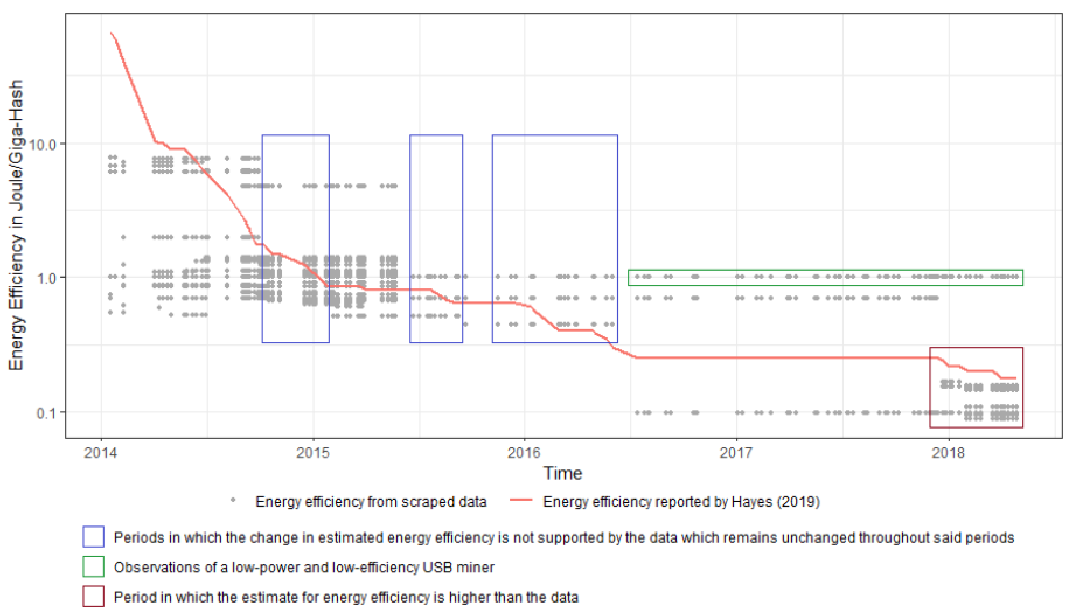
One of the most important parameters of the CPM described by Equations (1)–(3) is the energy efficiency of the mining equipment for the whole Bitcoin network. Finding a reliable estimate for this parameter is a very challenging task due to the scarcity of data for most mining pools, if not the complete lack of data. Hayes (2019) computed this parameter by extracting energy efficiency data from Bitcoin mining hardware manufacturer websites and by checking them against a dedicated wiki page that catalogs the efficiency of the mining hardware (https://en.bitcoin.it/wiki/Mining_hardware_comparison). He then …“collected these data for each date of difficulty change in the Bitcoin network, scraped from the web using the internet archive’s wayback machine”. The network energy efficiency was finally computed using a power log-function applied to these data3. We tried to replicate and extend the Hayes’ estimated energy efficiency by web scraping data from the previous “Mining hardware comparison” webpage. However, when we overlaid the energy efficiency estimated by Hayes (2019) with the scraped ASIC data, we found some anomalies, see Figure 2: at the end of 2015 and until the beginning of 2016, the estimated energy efficiency suddenly changes but the ASIC release data do not. Moreover, during the first months of 2018, several new releases were introduced but the estimated energy efficiency always stays above these releases. Furthermore, there is a line of violet dots constant at 1 Joule/GH which corresponds to USB miners, which are no longer competitive products but they still seem to be included in the computation of the energy efficiency even in 2017–2018.
Given these issues, we decided to follow a different approach. First, we examined a couple of websites that catalog the bitcoin mining equipment (see ASIC Miner Value 2020 and Crypto Mining Tools 2020), and we scraped their data and cross-checked it with vendor websites and online marketplaces to find any possible discrepancies. Then, following the idea proposed by Stoll et al. (2019) to compute lower and upper bands for the energy efficiency, we decided to use two alternative Holt-Winters double exponential smoothing with the scraped data to model the dynamics of the energy efficiency for the whole Bitcoin network. We chose this kind of methodology for the following reasons:
- This type of smoothing naturally trails the data and it can model the gradual replacement of old equipment with the new one. Changing the coefficients of the smoothing function impacts the length of such lag.
- It accounts for a trend that is present in the data.
- The energy efficiency of future ASICs cannot be used to infer today’s performance, so any smoothing function referring to future values cannot be used.
The Holt-Winters double exponential smoothing function and its parameters for two alternative models are reported below:
where is the raw data sequence of ASICs energy efficiencies (measured in Joule/Giga-Hash), is the smoothed value at time t and it represents an estimate of the energy efficiency for the whole Bitcoin network, while is the estimate of the trend at time t. The parameters for the two alternative smoothing models were chosen to give the equipment a reasonable replacement rate of 2–3 months4, and to get two smoothed curves: one with slow and smooth energy efficiency development over time and the other with more abrupt changes around the release dates of new hardware. Using this approach, we computed the change of the network energy efficiency over time that is reported in Figure 3.
3.2. The Cost-of-Production Model and Electricity Prices
The electricity price was fixed to a constant (0.13 dollars per kWh), similarly to Hayes (2017, 2019). Even though the actual electricity price might be lower for miners—after all, they are active seekers of cheap electricity—we chose this level for two reasons: (1) there is no better-educated guess; (2) if we assume electricity prices which are potentially higher than the real ones, we can capture the effect of some other mining operational expenses, as discussed by Stoll et al. (2019). This assumption will be relaxed in Section 5, where we will discuss a robustness check involving electricity prices changing every day.
3.3. The Cost-of-Production Model and the Bitcoin Reward Halving
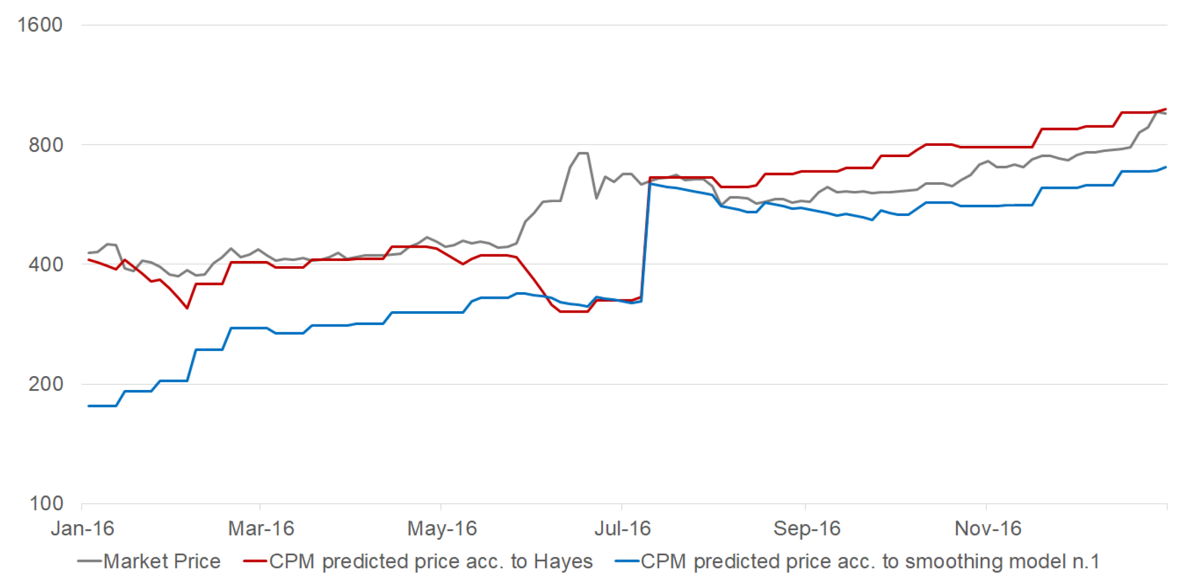
The bitcoin halving happens once approximately every four years and cuts the block reward (and thus the future cash flows of miners) in half. The cost-of-production model does not account for this effect, but miners are aware of it and anticipate it. This is why the market price does not change significantly near the times of halving, whereas the cost-of-production model shows a sudden break in its equilibrium price. This effect is shown in Figure 4 where a cost-of-production model is considered with two different inputs for the network energy efficiency: one as originally published by Hayes (2019) and another estimated using the first smoothing model in Equation (4).
Even though the two models differ due to the different methodologies used for computing the network energy efficiency, they both show the same jump in prices at the time of the halving event in July 2016. It is for this reason that our empirical analysis considered only bitcoin market prices between August 2016 and February 2020 to exclude the two halving events which took place in July 2016 and May 2020, respectively. Accounting for these breaks and the change in miners’ behavior would have required additional assumptions and model complexities that would have probably weakened the overall analysis. This is why we leave it as an avenue for further research, and we refer the interested reader to Pagnotta and Buraschi (2018) and Pagnotta (2020) for two recent theoretical models dealing with this issue5 6.
4. Results
4.1. Data
The dataset examined in this paper consists of weekly data ranging from 1 August 2016 till 29 February 2020: similarly to Kjærland et al. (2018), we transformed the original daily data into weekly averages to avoid potential issues related to autocorrelation. The motivation for such a time sample was to get the most recent data but, at the same time, to avoid any bitcoin halving events: as we discussed in Section 3.3, the nature of these events is unique and should be studied separately.
The variables used in this paper and the reasons for using them largely follow Kjærland et al. (2018). However, there are also three important differences. First, we did not consider oil prices and VIX in our analysis: they were shown to be not statistically significant in Kjærland et al. (2018) and they kept being not significant in our study, so we preferred to have a smaller set of variables to increase the efficiency of our final estimates. Second, we added a variable measuring the transaction fees: this variable does not just show the public interest in bitcoin but rather reveals the real “invested” interest: that is, the actual amount of money that the users are willing to give up in commissions to move their bitcoins. Third, we consider the CPM estimated using the inputs discussed in Section 3 as an alternative to the hashrate. A description of the variables used in the empirical analysis is reported in Table 1, while their plots are reported in Figure 5. Instead, the cost-of-production model prices computed using the two smoothed energy efficiency curves discussed in Section 3.1 are shown in Figure 6, together with the bitcoin market price.
We analyzed the stationarity of our variables using a set of unit root tests allowing for a potential endogenous structural break, both under the null of a unit root and under the alternative. We justify this choice considering that there is literature showing that there was a financial bubble in the bitcoin prices in 2016–2017 that burst at the beginning of 2018, see Corbet et al. (2018); Fry (2018); Gerlach et al. (2019); and Xiong et al. (2020). Moreover, there is also a debate on whether the introduction of bitcoin futures in December 2017 crashed the market prices: in this regard, the evidence is more mixed with Hattori and Ishida (2020) concluding that bitcoin futures did not lead to the crash of the bitcoin market, whereas Liu et al. (2019) and Jalan et al. (2019) affirm that they were to an extent responsible for the crash of bitcoin prices in 2018. However, Baig et al. (2020) and Köchling et al. (2019) showed that the introduction of bitcoin futures indeed improved the efficiency of the bitcoin markets. Given this evidence, we employed two types of unit root tests: the Vogelsang and Perron (1998) test and the Lee and Strazicich (2003) test, both of them allowing for one endogenous break. The results of these tests for the log-transformed variables and their log-returns are reported in Table 2.
The results in Table 2 show that all time series are not stationary, with structural breaks mainly located at the end of 2017 (particularly for bitcoin-related variables), which is consistent with the past financial literature dealing with bitcoin prices. Given this evidence, we fixed a break date on 10 December 2017, which is the day when the first bitcoin futures were introduced on the CBOE, and we divided our dataset into two samples: 01/08/2016–04/12/2017 and 11/12/2017–24/02/2020. The next steps of our empirical analysis were then performed with these samples separately.
4.2. Bivariate Analysis
The next step of our investigation was to test for cointegration (in all subsamples) between the market price and the cost-of-production price or between the market price and the hashrate. We also tested for Granger causality using the approach by Toda and Yamamoto (1995), which is consistent even if the processes may be integrated or cointegrated of arbitrary order. Note that the Granger representation theorem by Engle and Granger (1987) assures us that if two or more time-series are cointegrated, then there must be Granger causality between them because the error correction term enters at least one of the equations of the error correction model. However, the presence of Granger causality (either one-way or in both directions) does not necessarily imply that the series are cointegrated, see Lütkepohl (2005)-chapters 6–7 and references therein for more details. The results of the Granger causality tests using the Toda and Yamamoto (1995) approach and of the bivariate Johansen cointegration tests are reported in Table 3 and Table 4, respectively.
Table 3 and Table 4 show that there is neither evidence of Granger-causality nor cointegration in the first sample (01/08/2016–04/12/2017), whereas there is evidence of unidirectional Granger-causality and cointegration in the second sample (11/12/2017–24/02/2020), going from the bitcoin price to the hashrate (or to the CPM) but not vice versa. The final estimated bivariate models for both subsamples are reported in Table A1, Table A2, Table A3, Table A4, Table A5 and Table A6 in Appendix B, while the misspecification tests for these models are reported in Table 57. In this regard, we computed the following battery of misspecification tests with the models’ residuals: the multivariate Lagrange Multiplier (LM) test for residual serial correlation up to a specified order, the multivariate Jarque-Bera normality test, and the multivariate White heteroskedasticity test, see Johansen (1995) and Lütkepohl (2005) for more details. We also calculated the BDS test by Broock et al. (1996) to test whether the residuals are independent and identically distributed (iid) and which is robust against a variety of possible deviations from independence, including linear dependence, nonlinear dependence, or chaos. Finally, we computed block exogeneity Wald tests to check whether the bitcoin price can be treated as exogenous, by testing for the joint significance of each of the other lagged endogenous variables in the bitcoin equation (provided that lagged variables are present). If VECMs were used, we also tested that the factor loading associated with the error correction term in the bitcoin equation was not statistically different from zero. For ease of reference, we referred to the block exogeneity Wald test in Table 5 as short-run, while to the test on the factor loading as long-run.
Table A1, Table A2, Table A3, Table A4, Table A5, Table A6 and Table 5 show that simple bivariate random walk models and a VAR(1) for log-returns were sufficient to model the weak dynamics of the bitcoin prices and the hashrate/CPMs in the first sample, while vector error correction models (VECMs) were used in the second sample. It is possible to note that the hashrate and the CPMs did not have any effect on the bitcoin price in any period and model, whereas the bitcoin price affected the hashrate/CPMs with lags ranging from one week up to six weeks later, depending on the model specification. Interestingly, the models using the hashrate showed always better misspecification tests than those using the CPMs. Moreover, the lagged effects of bitcoin prices on the hashrate were generally longer than the same effects on the CPMs, and these longer lags are more realistic given that it takes time to update the mining equipment. Therefore, this initial bivariate evidence seems to highlight that it is better to consider the hashrate directly rather than its proxy represented by the bitcoin cost-of-production model when modeling its relationship with the bitcoin price.
4.3. Multivariate Analysis
The next step in our analysis was to select the best multivariate model using the structural relationship identification methodology suggested by Sa-ngasoongsong et al. (2012) and Fantazzini and Toktamysova (2015) and the variables described in Section 4.1. The results of the sequential reduction method for weak exogeneity using the Wald test by Toda and Yamamoto (1995) are reported in Table 6: only Google search data and transaction fees were found to be endogenous during the first subsample (01/08/2016–04/12/2017), while the transaction volume, the hashrate, and the CPMs 1 and 2 were endogenous variables in the second subsample (11/12/2017–24/02/2020). We then proceeded to test for cointegration using the variables which were deemed endogenous according to the previous sequential test procedure, and the results of the Johansen cointegration tests are reported in Table 7. The final estimated multivariate models for both subsamples are reported in Table A7, Table A8, Table A9, and Table A10 in Appendix B, while the misspecification tests for these models are reported in Table 8.
In the first subsample, the hashrate and the CPM1/CPM2 were never significant, neither as endogenous nor as exogenous variables, and the final model was a bivariate VECM(1) for the Bitcoin price and Google search data, with transaction volume and transaction fees as exogenous variables. The bitcoin price was found again to be weakly exogenous, and the direction of causality was from the bitcoin price to the Google search data. Similarly to the bivariate analysis, a significant cointegration relationship was found in the second subsample between the bitcoin price and the hashrate or its proxies, while Google data, transaction volume, and transaction fees were found mostly to be significant exogenous variables. Again, the model using the hashrate showed better misspecification tests than those using the CPMs, and the lagged effects of bitcoin prices on the hashrate were generally longer than the same effects on the CPMs. No particular difference was found when using the CPM1 or the CPM2. Therefore, this multivariate evidence confirms the previous bivariate analysis, showing that it is better to consider directly the hashrate rather than its proxy represented by the bitcoin cost-of-production model when modeling its relationship with the bitcoin price. Moreover, the causality is always unidirectional going from the bitcoin price to the hashrate/CPM1/CPM2, with lags ranging from one week up to six weeks later. Furthermore, this evidence confirmed that there was a sharp change in market behavior from the first period to the second one, thus corroborating the past financial literature. The burst of the bubble at the end of 2017 and the simultaneous introduction of bitcoin futures represented a major change in the market dynamics, by filtering the group of bitcoin traders (only those better informed and financially robust survived the market crash) and by improving the market efficiency, respectively.
These findings are consistent with a large literature in energy economics, which showed that oil and gas returns affect the purchase of the drilling rigs with a delay of up to three months, whereas the impact of changes in the rig count on oil and gas returns is limited or not significant, see Khalifa et al. (2017) for a large discussion and a detailed review of this literature. Differently from Khalifa et al. (2017) who found a nonlinear relationship, with oil returns affecting changes in rig counts much stronger when the oil returns take on very negative values, the BDS tests on our models’ residuals did not highlight any strong missing nonlinearity. We also tested our data for nonlinear Granger causality using the test implemented in the NlinTS R package by Hmamouche (2020) that is based on Schreiber (2000) and Kraskov et al. (2004), as well as for threshold nonlinear cointegration using the Seo (2006) test, but we did not find any significant evidence of nonlinearity8. This difference can probably be explained by the relatively small dimension of our dataset (2016–2020) compared to the one used by Khalifa et al. (2017) (1990–2015). Moreover, Khalifa et al. (2017) showed that the evidence of nonlinearity has softened in the most recent years, and similar evidence was also reported by Ansari and Kaufmann (2019) who used a linear cointegrated model.
5. Robustness Checks
We wanted to check how our previous results changed when computing the bitcoin cost-of-production using an electricity price no more fixed to a constant but able to reflect the changing dynamics of daily electricity markets. To achieve this goal, we employed the daily data of the Nord pool9 system price, which is the unconstrained market clearing reference price for the European Nordic region, computed without any congestion restrictions by setting capacities to infinity10. These daily prices (originally in Euro/MWh) were transformed into $/kWh using the daily fixing of the EURUSD pair, and they are shown in Figure 7.
The Nord Pool is particularly interesting in our case because it reflects the increasing importance of renewable energy in the European energy mix (see Jones 2017-chapter 5 for a discussion at the textbook level), and the “majority of Bitcoin mining is mainly powered by what would otherwise be a wasted surplus of renewable energy” (de Vries 2019), particularly hydro-power, see Bendiksen et al. (2018) for the full details.
The CPMs computed using the Nord Pool electricity prices and the two energy efficiency curves presented in Section 3.1 as well as the CPMs computed with constant electricity prices are reported in Figure 8, together with the bitcoin market prices.
The CPMs computed using Nord Pool electricity prices are much lower than the CPMs computed with a fixed electricity price of 0.13 $/kWh, because Nord Pool prices are significantly lower than this constant price level. As we discussed in Section 3.2, an higher electricity price can capture the effect of some other mining operational expenses, so the CPMs computed using Nord Pool prices can be considered as proxies for the marginal cost of production, see Fantazzini (2019)-chapter 4 for a broad discussion of this issue.
The results of the sequential reduction method for weak exogeneity using the Wald test by Toda and Yamamoto (1995) and the CPMs using Nord Pool prices are reported in Table A11 (Appendix B), while the results of the Johansen cointegration tests are reported in Table A12 (Appendix B). The misspecification tests for the final selected models are reported in Table A13 (Appendix B)11.
The results using the CPMs with the Nord pool prices are not very dissimilar from the baseline case: in the first subsample, the CPM1/CPM2 were never significant, and the final model was again a bivariate VECM(1) for the Bitcoin price and Google search data, with transaction volume and transaction fees as exogenous variables. In the second subsample, there were no endogenous variables according to the sequential reduction method for weak exogeneity, and the Johansen tests similarly found no evidence of cointegration between the bitcoin market price and the CPMs. The final models turned out to be a simple bivariate random walk (VAR(0)) and a VAR(4) model for the log-returns of the bitcoin price and the CPM1/CPM2, respectively, with misspecification tests slightly worse than the baseline case.
In general, the use of the Nord Pool prices to compute the CPMs tend to soften their relationship with the bitcoin market price: this fact is already evident when looking at the correlation matrices of the log-returns for the bitcoin price, the baseline CPMs, and the CPMs computed with the Nord pool prices, which are reported in Table A14 in Appendix B.
6. Conclusions
This paper investigated the relationship between the bitcoin price and the hashrate by disentangling the effects of the energy efficiency of the bitcoin mining equipment, bitcoin halving, and of structural breaks on the price dynamics. To reach this aim, we proposed a new methodology based on exponential smoothing to model the dynamics of the Bitcoin network energy efficiency. We considered either directly the hashrate or the bitcoin cost-of-production model by Hayes (2017, 2019) as a proxy for the hashrate, to take any nonlinearity into account. We found that there was neither evidence of Granger-causality nor cointegration in the first examined sample (01/08/2016–04/12/2017), whereas there was evidence of unidirectional Granger-causality and cointegration in the second sample (11/12/2017–24/02/2020), going from the bitcoin price to the hashrate (or to the CPMs) but not vice versa. This evidence is thus consistent with a large literature in energy economics, which showed that oil and gas returns affect the purchase of the drilling rigs with a delay of up to three months, whereas the impact of changes in the rig count on oil and gas returns is limited or not significant. Moreover, our analysis showed that it is better to consider directly the hashrate rather than its proxy represented by the bitcoin cost-of-production model when modeling its relationship with the bitcoin price. These results also held after we performed a robustness check to verify how our previous results changed when computing the bitcoin cost-of-production using an electricity price no more fixed to a constant but equal to the daily data of the Nord pool system price.
The evidence reported in this work shows that the bitcoin market has become a more mature and efficient market after the introduction of regulated futures markets in December 2017. The usual technical drivers (bitcoin supply and demand), attractiveness indicators, and macroeconomic variables appear to have become either lagging indicators or no more significant in explaining the dynamics of the bitcoin price, thus confirming similar results reported by Kapar and Olmo (2020). In this regard, we want to remark that Shanaev et al. (2019) recently showed that some of the previously reported positive relationships between crypto-coins prices and their hashrate, or between crypto-coins prices and their transaction counts, were either spurious due to serial correlation or inconsistent due to endogeneity. Therefore, the development of “second-generation valuation metrics” for cryptocurrencies (Lehner et al. 2019; Shanaev et al. 2019) able to accommodate both modern empirical finance asset-pricing models and theory-driven valuation models is definitively a compelling avenue for further research.
Author Contributions
Conceptualization, N.K.; Methodology, N.K. and D.F.; software, N.K. and D.F.; validation, N.K. and D.F.; formal analysis, N.K. and D.F. investigation, N.K. and D.F.; resources, N.K. and D.F.; data curation, N.K. and D.F.; writing–original draft preparation, N.K. and D.F.; writing–review and editing, D.F.; visualization, N.K. and D.F.; supervision, D.F.; project administration, D.F.; funding acquisition, D.F. All authors have read and agreed to the published version of the manuscript.
Funding
This research was funded by Dean Fantazzini grant number 20-68-47030.
Acknowledgments
We would like to thank all the participants of the VII International Conference in Modern Econometric Tools and Applications (META2020), which was held in September 2020 and was organized by the Higher School of Economics in Nizhny Novgorod (Russia). We also want to thank Sergei Tikhomirov, an anonymous founder of a crypto-exchange, and the anonymous chief information officer (CIO) of one of the world’s leading full-service blockchain technology companies, who provided important feedback. The first-named author gratefully acknowledges financial support from the grant of the Russian Science Foundation n. 20-68-47030.
Conflicts of Interest
The authors declare no conflict of interest.
Appendix A. A Brief Overview of Bitcoin’s Operation
The complete description of how the Bitcoin network works can be found in the original whitepaper published by Nakamoto (2008) and it is beyond the scope of this paper. However, certain aspects of its operation are briefly reviewed here to better understand the research discussed in this paper. The bitcoin supply is completely inelastic, and it is determined by a fixed emission schedule: for the first four years, 50 bitcoins are created on average every 10 min. After the first four years, the rate of emission halves, and only 25 bitcoins appear within the network every 10 min. The creation of bitcoin is again halved every four years, and this pattern is repeated until the smallest possible unit is created 12. and, after this event, the emissions stop completely. The total amount of bitcoin to be created will be equal to 21 million bitcoin. Due to the nature of the bitcoin protocol, the rate of emission cannot be manipulated or altered in any way, so that we already know that emission of bitcoin will cease in the year 2140.
Newly created bitcoins come with what is called a block: a chunk of transactions “packaged” in a special way. The size of each block is limited, so there is a competition among those using the Bitcoin network to have their transactions inserted into the earliest block, which gives rise to a fee market. There is also a competition to confirm the latest transactions and produce a new block: this process is incentivized by the (1) reward offered by the Bitcoin network (for being the first to confirm a new block) and by the (2) fees collected from all transactions included in the block. To control the rate of the block issuance, the bitcoin protocol has certain rules in place. Each newly created block has to provide a so called proof of work to be considered valid. The proof of work is a hard, unforgeable digital evidence of the “work” performed to confirm a block of transactions. In other words, to create a valid block, one has to expend a certain amount of computational resources and then presents the evidence of that expenditure within the block. Given that the combined computational power of all those interested in creating a block may increase or decrease, the Bitcoin network has a concept of difficulty: it tells how much computations on average a miner has to do before he gets a valid proof of work. If the total computational power in the network suddenly surges, blocks start to come out at a higher rate: the network notices that and readjusts the difficulty target to slow the rate back down. Thus, the average time between the blocks is always kept at 10 min, independently from the changes in the total computational power. The process of providing the proof of work for a block is called mining and its participants are called miners. The equipment used by miners is usually called “miners” as well. Today such equipment is dominated by application-specific integrated circuit (ASIC) chips.
The computations that miners do involve a double SHA-256 hash function, so the computational power is often called hashrate and is measured in hashes per second. The miners are always in an arms race for higher energy efficiency (EEF) of their ASICs and for a higher number of hashes per second (usually measured in Ghash/sec). The current state of the network is such that even a large miner can only hope to find a block once every year or so. Because of that, miners pool their efforts together to increase their combined hashrate and hope to find blocks at a much faster and steadier rate. The pool operators coordinate the miners and take a small management fee for that. In this way, an individual miner gives up some of his expected profit in exchange for steady and predictable payouts. Each miner incurs certain costs when mining for a block: these costs are both fixed (real estate, equipment, set-up costs) and variable (energy, labor, cooling, etc.). By far, energy costs are the highest cost: they may be so big that other costs might be safely neglected, see Stoll et al. (2019) for more details.
Due to the nature of the Bitcoin network, some of its parameters can be directly observed and their past values are forever kept in its public blockchain: see, for example, the block reward, the total transaction fees Blockchain.com (2020c), the hashrate Blockchain.com (2020b), and the difficulty Blockchain.com (2020a). They are widely used in bitcoin-related research.
Appendix B. Model Estimates
Each equation is reported by column, while each cell reports the parameter estimate, its standard error, and t-statistic.
Appendix B.1. Bivariate Analysis

Table A1.
VAR(0) for the Log-returns of the pair: Log(Bitcoin price), Log(CPM model 1). First sample: 01/08/2016–04/12/2017.
Table A1.
VAR(0) for the Log-returns of the pair: Log(Bitcoin price), Log(CPM model 1). First sample: 01/08/2016–04/12/2017.
| Variables | DLog(Bitcoin Price) | DLog(CPM_model_1) |
|---|---|---|
| Constant | 0.046586 | 0.019783 |
| −0.01353 | −0.0046 | |
| [3.44263] | [4.30423] |
Table A2.
VAR(0) for the Log-returns of the pair: Log(Bitcoin price), Log(CPM model 2). First sample: 01/08/2016–04/12/2017.
Table A2.
VAR(0) for the Log-returns of the pair: Log(Bitcoin price), Log(CPM model 2). First sample: 01/08/2016–04/12/2017.
| Variables | DLog(Bitcoin Price) | DLog(CPM_model_2) |
|---|---|---|
| Constant | 0.046586 | 0.021165 |
| −0.01353 | −0.00536 | |
| [3.44263] | [3.94997] |
Table A3.
VAR(1) for the Log-returns of the pair: Log(Bitcoin price), Log(Hashrate). First sample: 01/08/2016–04/12/2017.
Table A3.
VAR(1) for the Log-returns of the pair: Log(Bitcoin price), Log(Hashrate). First sample: 01/08/2016–04/12/2017.
| Variables | DLog(Bitcoin Price) | DLog(Hashrate) |
|---|---|---|
| DLog(Bitcoin price(−1)) | 0.011607 | −0.02143 |
| −0.13052 | −0.16834 | |
| [0.08893] | [−0.12730] | |
| DLog(Hashrate(−1)) | −0.08538 | −0.596435 |
| −0.07991 | -0.10306 | |
| [−1.06849] | [−5.78708] | |
| Constant | 0.049622 | 0.047781 |
| −0.01481 | −0.0191 | |
| [3.35113] | [2.50179] |
Table A4.
VECM(0) for the variables Log(Bitcoin price) and Log(CPM model 1). Second sample: 11/12/2017–24/02/2020.
Table A4.
VECM(0) for the variables Log(Bitcoin price) and Log(CPM model 1). Second sample: 11/12/2017–24/02/2020.
| Error Correction (EC) Term | ||
|---|---|---|
| Log(Bitcoin price(−1)) | 1 | |
| Log(CPM_model_1(−1)) | −0.663981 | |
| −0.21282 | ||
| [−3.11985] | ||
| Constant | −2.97009 | |
| −1.81363 | ||
| [−1.63765] | ||
| Variables | DLog(Bitcoin price) | DLog(CPM_model_1) |
| EC | −0.03118 | 0.044423 |
| −0.01726 | −0.00559 | |
| [−1.80600] | [7.95227] |
Table A5.
VECM(2) for the variables Log(Bitcoin price) and Log(CPM model 2). Second sample: 11/12/2017–24/02/2020.
Table A5.
VECM(2) for the variables Log(Bitcoin price) and Log(CPM model 2). Second sample: 11/12/2017–24/02/2020.
| Error Correction (EC) Term | ||
|---|---|---|
| Log(Bitcoin price(−1)) | 1 | |
| Log(CPM_model_2(−1)) | −0.692219 | |
| −0.21357 | ||
| [−3.24116] | ||
| Constant | −2.806945 | |
| −1.84646 | ||
| [−1.52017] | ||
| Variables | D(Log(Bitcoin price)) | D(Log(CPM_model_2)) |
| EC | −0.029855 | 0.042844 |
| −0.03116 | −0.01095 | |
| [−0.95809] | [3.91310] | |
| 0.098178 | 0.02819 | |
| D(Log(Bitcoin price(−1))) | −0.09641 | −0.03388 |
| [1.01832] | [0.83217] | |
| −0.039484 | 0.045213 | |
| D(Log(Bitcoin price(−2))) | −0.09497 | −0.03337 |
| [−0.41575] | [1.35492] | |
| −0.004661 | 0.171544 | |
| D(Log(CPM_model_2(−1))) | −0.24632 | −0.08655 |
| [−0.01892] | [1.98206] | |
| −0.05507 | 0.274415 | |
| D(Log(CPM_model_2(−2))) | −0.23794 | −0.0836 |
| [−0.23145] | [3.28235] |
Table A6.
VECM(6) for Log(Bitcoin price) and Log(Hashrate). Second sample: 11/12/2017–24/02/2020.
| Error Correction (EC) Term | ||
|---|---|---|
| Log(Bitcoin price(−1)) | 1 | |
| Log(Hashrate(−1)) | −0.409183 | |
| −0.1125 | ||
| [−3.63727] | ||
| Constant | −1.256762 | |
| −2.00595 | ||
| [−0.62652] | ||
| Variables | D(Log(Bitcoin price)) | D(Log(Hashrate)) |
| EC | −0.049126 | 0.147903 |
| −0.02597 | −0.02708 | |
| [−1.89180] | [ 5.46226] | |
| D(Log(Bitcoin price(−1))) | 0.183584 | −0.050318 |
| −0.09211 | −0.09605 | |
| [1.99306] | [−0.52390] | |
| D(Log(Bitcoin price(−2))) | −0.032037 | 0.157578 |
| −0.08781 | −0.09156 | |
| [−0.36485] | [1.72106] | |
| D(Log(Bitcoin price(−3))) | 0.108266 | 0.04156 |
| −0.08754 | −0.09127 | |
| [1.23682] | [0.45532] | |
| D(Log(Bitcoin price(−4))) | −0.14961 | −0.149548 |
| −0.08646 | −0.09016 | |
| [−1.73033] | [−1.65877] | |
| D(Log(Bitcoin price(−5))) | −0.034145 | 0.077298 |
| −0.08735 | −0.09108 | |
| [−0.39092] | [0.84871] | |
| D(Log(Bitcoin price(−6))) | 0.170596 | 0.072128 |
| −0.08667 | −0.09038 | |
| [1.96824] | [0.79808] | |
| D(Log(Hashrate(−1))) | −0.076181 | −0.736701 |
| −0.08894 | −0.09273 | |
| [−0.85659] | [−7.94419] | |
| D(Log(Hashrate(−2))) | 0.009311 | −0.438379 |
| −0.10961 | −0.11429 | |
| [0.08495] | [−3.83559] | |
| D(Log(Hashrate(−3))) | 0.099676 | −0.273345 |
| −0.11133 | −0.11608 | |
| [0.89533] | [−2.35471] | |
| D(Log(Hashrate(−4))) | 0.105471 | −0.275003 |
| −0.11083 | −0.11556 | |
| [0.95169] | [−2.37976] | |
| D(Log(Hashrate(−5))) | −0.005624 | −0.29404 |
| −0.1056 | −0.11011 | |
| [−0.05326] | [−2.67035] | |
| D(Log(Hashrate(−6))) | 0.171554 | −0.154059 |
| −0.08442 | −0.08803 | |
| [2.03213] | [−1.75014] |
Appendix B.2. Multivariate Analysis
Table A7.
VECMX(1) for Log(Bitcoin price) and Log(Google), with Log(transaction volume) and Log(Transaction fees) as exogenous variables. First sample: 01/08/2016–04/12/2017. This model turned out to be the same, independently of whether we used the hashrate, or the CPM1, or the CPM2.
Table A7.
VECMX(1) for Log(Bitcoin price) and Log(Google), with Log(transaction volume) and Log(Transaction fees) as exogenous variables. First sample: 01/08/2016–04/12/2017. This model turned out to be the same, independently of whether we used the hashrate, or the CPM1, or the CPM2.
| Error Correction (EC) Term | ||
|---|---|---|
| Log(Bitcoin price(−1)) | 1 | |
| Log(Google(−1)) | −1.000538 | |
| −0.04603 | ||
| [−21.7368] | ||
| Constant | −5.4321 | |
| Variables | D(Log(Bitcoin price)) | D(Log(Google)) |
| EC | −0.020082 | 0.604649 |
| −0.05422 | −0.12658 | |
| [−0.37039] | [4.77691] | |
| D(Log(Bitcoin price(−1))) | −0.071363 | 0.143743 |
| −0.09649 | −0.22527 | |
| [−0.73957] | [0.63810] | |
| D(Log(Google(−1))) | −0.012273 | 0.134782 |
| −0.04903 | −0.11446 | |
| [−0.25031] | [1.17753] | |
| Constant | 0.02109 | 0.010608 |
| −0.01033 | −0.02413 | |
| [2.04073] | [0.43967] | |
| D(Log(Transaction fees)) | 0.172323 | 0.040111 |
| −0.04195 | −0.09793 | |
| [4.10790] | [0.40958] | |
| D(Log(Transaction Volume)) | 0.335968 | 0.443305 |
| −0.06704 | −0.15652 | |
| [5.01110] | [2.83227] |
Table A8.
VECMX(6) for Log(Bitcoin price), Log(Hashrate) and Log(Transaction fees), with Log(transaction volume), Log(Google), and Log(Transaction fees) as exogenous variables. Second sample: 11/12/2017-24/02/2020.
Table A8.
VECMX(6) for Log(Bitcoin price), Log(Hashrate) and Log(Transaction fees), with Log(transaction volume), Log(Google), and Log(Transaction fees) as exogenous variables. Second sample: 11/12/2017-24/02/2020.
| Error Correction (EC) Term | ||
|---|---|---|
| Log(Bitcoin price(−1)) | 1 | |
| Log(Hashrate(−1)) | −0.442911 | |
| −0.12766 | ||
| [−3.46936] | ||
| Constant | −0.620773 | |
| −2.27623 | ||
| [−0.27272] | ||
| Variables | D(Log(Bitcoin price)) | D(Log(Hashrate)) |
| EC | −0.009204 | 0.143938 |
| −0.01909 | −0.02662 | |
| [−0.48217] | [ 5.40721] | |
| D(Log(Bitcoin price(−1))) | 0.105778 | −0.053536 |
| −0.07226 | −0.10077 | |
| [1.46388] | [−0.53126] | |
| Variables | D(Log(Bitcoin price)) | D(Log(Hashrate)) |
| D(Log(Bitcoin price(−2))) | 0.032122 | 0.159914 |
| −0.06866 | −0.09575 | |
| [0.46786] | [ 1.67010] | |
| D(Log(Bitcoin price(−3))) | −0.026725 | 0.040566 |
| −0.06826 | −0.0952 | |
| [−0.39151] | [ 0.42612] | |
| D(Log(Bitcoin price(−4))) | −0.04931 | −0.138195 |
| −0.06636 | −0.09255 | |
| [−0.74303] | [−1.49317] | |
| D(Log(Bitcoin price(−5))) | −0.064049 | 0.073961 |
| −0.06817 | −0.09507 | |
| [−0.93961] | [0.77800] | |
| D(Log(Bitcoin price(−6))) | 0.132207 | 0.070274 |
| −0.06677 | −0.09312 | |
| [ 1.97995] | [0.75465] | |
| D(Log(Hashrate(−1))) | −0.119478 | −0.741459 |
| −0.06751 | −0.09415 | |
| [−1.76969] | [−7.87490] | |
| D(Log(Hashrate(−2))) | −0.016763 | −0.442022 |
| −0.08292 | −0.11564 | |
| [−0.20217] | [−3.82241] | |
| D(Log(Hashrate(−3))) | 0.077149 | −0.277793 |
| −0.08467 | −0.11808 | |
| [0.91118] | [−2.35258] | |
| D(Log(Hashrate(−4))) | −0.033626 | −0.285352 |
| −0.08528 | −0.11893 | |
| [−0.39432] | [−2.39936] | |
| D(Log(Hashrate(−5))) | −0.035212 | −0.297643 |
| −0.08005 | −0.11164 | |
| [−0.43989] | [−2.66622] | |
| D(Log(Hashrate(−6))) | 0.075737 | −0.157866 |
| −0.06518 | −0.09091 | |
| [1.16190] | [−1.73659] | |
| DLog(Google) | −0.164882 | 0.015363 |
| −0.04637 | −0.06467 | |
| [−3.55586] | [0.23757] | |
| DLog(Transaction fees) | 0.074418 | 0.004869 |
| −0.02798 | −0.03902 | |
| [2.65972] | [0.12477] | |
| DLog(Transaction Volume) | 0.326196 | 0.020172 |
| −0.04868 | −0.06789 | |
| [6.70053] | [0.29711] |
Table A9.
VECMX(2) for Log(Bitcoin price), Log(CPM model 1), and Log(Transaction volume), with Log(transaction fees), Log(Google), and Log(SP500) as exogenous variables. Second sample: 11/12/2017–24/02/2020.
Table A9.
VECMX(2) for Log(Bitcoin price), Log(CPM model 1), and Log(Transaction volume), with Log(transaction fees), Log(Google), and Log(SP500) as exogenous variables. Second sample: 11/12/2017–24/02/2020.
| Error Correction (EC) Term | |||
|---|---|---|---|
| Log(Bitcoin price(−1)) | 1 | ||
| Log(CPM_model_1(−1)) | −0.631559 | ||
| −0.07653 | |||
| [−8.25280] | |||
| Log(Transaction Volume(−1)) | −0.767616 | ||
| −0.06355 | |||
| [−12.0782] | |||
| Constant | 12.95172 | ||
| −1.78079 | |||
| [7.27301] | |||
| Variables | D(Log(Bitcoin price)) | D(Log(CPM_model_1)) | D(Log(Transaction Volume)) |
| EC | 0.012154 | 0.144569 | 0.024845 |
| −0.07358 | −0.02403 | −0.11201 | |
| [0.16519] | [6.01564] | [0.22181] | |
| D(Log(Bitcoin price(−1))) | −0.033971 | −0.051945 | 0.214159 |
| −0.13416 | −0.04382 | −0.20424 | |
| [−0.25321] | [−1.18544] | [1.04859] | |
| D(Log(Bitcoin price(−2))) | −0.080567 | 0.02964 | −0.16257 |
| −0.11971 | −0.0391 | −0.18223 | |
| [−0.67304] | [0.75810] | [−0.89212] | |
| D(Log(CPM_model_1(−1))) | −0.222182 | −0.052122 | 0.520264 |
| −0.25878 | −0.08452 | −0.39394 | |
| [−0.85858] | [−0.61668] | [1.32066] | |
| D(Log(CPM_model_1(−2))) | −0.175314 | 0.122105 | −0.855809 |
| −0.25048 | −0.08181 | −0.38131 | |
| [−0.69991] | [1.49252] | [−2.24437] | |
| D(Log(Transaction Volume(−1))) | −0.000195 | 0.05502 | −0.342822 |
| −0.08185 | −0.02673 | −0.1246 | |
| [−0.00238] | [2.05804] | [−2.75130] | |
| D(Log(Transaction Volume(−2))) | −0.011235 | 0.028662 | −0.220672 |
| −0.07227 | −0.0236 | −0.11002 | |
| [−0.15546] | [1.21424] | [−2.00577] | |
| DLog(Transaction fees) | 0.170783 | −0.007478 | 0.27153 |
| −0.03007 | −0.00982 | −0.04578 | |
| [5.67931] | [−0.76138] | [5.93147] | |
| DLog(Google) | −0.139925 | 0.013245 | 0.106468 |
| −0.05695 | −0.0186 | −0.0867 | |
| [−2.45686] | [0.71203] | [1.22800] | |
| DLog(SP500) | 0.323125 | 0.287191 | 0.429537 |
| −0.38611 | −0.12611 | −0.58779 | |
| [0.83686] | [2.27729] | [0.73077] |
Table A10.
VECMX(2) for Log(Bitcoin price) and Log(CPM model 2), with Log(transaction fees), Log(Google), and Log(Transaction volume) as exogenous variables. Second sample: 11/12/2017–24/02/2020.
Table A10.
VECMX(2) for Log(Bitcoin price) and Log(CPM model 2), with Log(transaction fees), Log(Google), and Log(Transaction volume) as exogenous variables. Second sample: 11/12/2017–24/02/2020.
| Error Correction (EC) Term | ||
|---|---|---|
| Log(Bitcoin price(−1)) | 1 | |
| Log(CPM_model_2(−1)) | −0.788774 | |
| −0.22735 | ||
| [−3.46937] | ||
| Constant | −1.965044 | |
| −1.96566 | ||
| [−0.99969] | ||
| Variables | D(Log(Bitcoin price)) | D(Log(CPM model 2)) |
| EC | −0.003327 | 0.04146 |
| −0.02119 | −0.01049 | |
| [−0.15697] | [3.95174] | |
| D(Log(Bitcoin price(−1))) | 0.054894 | 0.029597 |
| −0.07037 | −0.03484 | |
| [0.78005] | [0.84959] | |
| D(Log(Bitcoin price(−2))) | 0.054567 | 0.041797 |
| −0.0712 | −0.03525 | |
| [0.76640] | [1.18588] | |
| D(Log(CPM model 2(−1))) | −0.367229 | 0.173548 |
| −0.17893 | −0.08858 | |
| [−2.05231] | [1.95926] | |
| D(Log(CPM model 2(−2))) | 0.2832 | 0.287279 |
| −0.17388 | −0.08608 | |
| [1.62872] | [3.33752] | |
| D(Log(Google)) | −0.181629 | 0.030859 |
| −0.04477 | −0.02216 | |
| [−4.05680] | [1.39236] | |
| DLog(Transaction fees) | 0.072612 | −0.00575 |
| −0.02712 | −0.01342 | |
| [2.67784] | [−0.42836] | |
| DLog(Transaction Volume) | 0.372787 | 0.000915 |
| −0.04758 | −0.02355 | |
| [7.83514] | [0.03883] |
Appendix B.3. Robustness Checks
Table A11.
Weak exogeneity tests: variables for which the null hypothesis of weak exogeneity can be rejected after re-testing at the 5% probability level.
Table A11.
Weak exogeneity tests: variables for which the null hypothesis of weak exogeneity can be rejected after re-testing at the 5% probability level.
| First sample: 01/08/2016–04/12/2017 | |||||
|---|---|---|---|---|---|
| Log(Transaction Fees) | Log(Transaction Volume) | Log(CPM_model_1) | Log(SP500) | Log(GOLD) | Log(Google) |
| V | |||||
| Log(Transaction Fees) | Log(Transaction Volume) | Log(CPM_model_2) | Log(SP500) | Log(GOLD) | Log(Google) |
| V | |||||
| Second sample: 11/12/2017–24/02/2020 | |||||
| Log(Transaction Fees) | Log(Transaction Volume) | Log(CPM_model_1) | Log(SP500) | Log(GOLD) | Log(Google) |
| Log(Transaction Fees) | Log(Transaction Volume) | Log(CPM_model_2) | Log(SP500) | Log(GOLD) | Log(Google) |
Table A12.
Multivariate Johansen cointegration tests. The null hypothesis is the absence of cointegration. The tests considered either the case of an intercept in the cointegration equa- tion (CE) and a trend in the variables (first sample) or the case of an intercept in the CE only (second sample). (*) The final model turned out to be the same, independently of whether we used the CPM1 or the CPM2.
| First Sample: | 01/08/2016–04/12/2017 |
|---|---|
| Variables | N. of CEs at 5% level |
| Log(Bitcoin_price), Log(Google) (*) | 1 |
| Second sample: | 11/12/2017–24/02/2020 |
| Variables | N. of CEs at 5% level |
| Log(Bitcoin_price), Log(CPM_model_1) | 0 |
| Log(Bitcoin_price), Log(CPM_model_2) | 0 |
Table A13.
Misspecification tests on the residuals from the multivariate models. p-values smaller than 5% are reported in bold font. (*) The final model turned out to be the same, independently of whether we used the CPM1 or the CPM2.
Table A13.
Misspecification tests on the residuals from the multivariate models. p-values smaller than 5% are reported in bold font. (*) The final model turned out to be the same, independently of whether we used the CPM1 or the CPM2.
| First Sample: 01/08/2016–04/12/2017 | ||
|---|---|---|
| Variables: | Variables: | |
| Log(Bitcoin_price), | Log(Bitcoin_price), | |
| Log(Google) (*) | Log(Google) (*) | |
| Model selected | VECMX(1) | VECMX(1) |
| Multivariate LM test (lag 4) | 0.99 | 0.99 |
| Multivariate LM test (lag 8) | 0.88 | 0.88 |
| Multivariate LM test (lag 12) | 0.45 | 0.45 |
| Multivariate White test | 0.10 | 0.10 |
| Multivariate Normality test | 0.00 | 0.00 |
| BDS (dim = 6) residuals 1st eq. | 0.53 | 0.53 |
| BDS (dim = 6) residuals 2nd eq. | 0.37 | 0.37 |
| Is bitcoin price weakly exogenous? | Yes (long-run: p value = 0.72) | Yes (long-run: p value = 0.72) |
| (short-run: p value = 0.83) | (short-run: p value = 0.83) | |
| Second sample: 11/12/2017–24/02/2020 | ||
| Variables: | Variables: | |
| Log(Bitcoin_price), | Log(Bitcoin_price), | |
| Log(CPM_model_1) | Log(CPM_model_2) | |
| Model selected | VAR(0) for log-returns | VAR(4) for log-returns |
| Multivariate LM test (lag 4) | 0.05 | 0.18 |
| Multivariate LM test (lag 8) | 0.29 | 0.17 |
| Multivariate LM test (lag 12) | 0.95 | 0.87 |
| Multivariate White test | 0.00 | 0.02 |
| Multivariate Normality test | 0.01 | 0.09 |
| BDS (dim = 6) residuals 1st eq. | 0.00 | 0.00 |
| BDS (dim = 6) residuals 2nd eq. | 0.00 | 0.00 |
| Is bitcoin price weakly exogenous? | Yes | Yes (short-run: p value = 0.16) |
Table A14.
Correlation matrices of the log-returns for the bitcoin price, the baseline CPMs with constant electricity, and the CPMs computed with the Nord pool prices.
Table A14.
Correlation matrices of the log-returns for the bitcoin price, the baseline CPMs with constant electricity, and the CPMs computed with the Nord pool prices.
| First Sample: 01/08/2016–04/12/2017 | |||||
|---|---|---|---|---|---|
| Bitcoin Market | CPM1 (constant | CPM2 (constant | CPM1 (Nord | CPM1 (Nord | |
| price | electricity price) | electricity price) | Pool price) | Pool price) | |
| Bitcoin Market p. | 1 | ||||
| CPM1 (constant e. p.) | 0.09 | 1 | |||
| CPM2 (constant e.p.) | 0.16 | 0.89 | 1 | ||
| CPM1 (Nord P. p.) | −0.08 | 0.12 | 0.12 | 1 | |
| CPM2 (Nord P. p.) | −0.04 | 0.13 | 0.22 | 0.98 | 1 |
| Second sample: 11/12/2017–24/02/2020 | |||||
| Bitcoin Market | CPM1 (constant | CPM2 (constant | CPM1 (Nord | CPM2 (Nord | |
| price | electricity price) | electricity price) | Pool price) | Pool price) | |
| Bitcoin Market p. | 1 | ||||
| CPM1 (constant e. p.) | −0.13 | 1 | |||
| CPM2 (constant e.p.) | −0.12 | 0.89 | 1 | ||
| CPM1 (Nord P. p.) | −0.07 | 0.40 | 0.42 | 1 | |
| CPM2 (Nord P. p.) | −0.07 | 0.42 | 0.51 | 0.98 | 1 |
References
- Ansari, Esmail, and Robert K. Kaufmann. 2019. The effect of oil and gas price and price volatility on rig activity in tight formations and opec strategy. Nature Energy 4: 321–28. [Google Scholar] [CrossRef]
- Aoyagi, Jun, and Takahiro Hattori. 2019. The Empirical Analysis of Bitcoin Market in the General Equilibrium Framework. Available online: https://papers.ssrn.com/sol3/papers.cfm?abstract_id=3433833 (accessed on 20 October 2020).
- ASIC Miner Value. 2020. Available online: https://www.asicminervalue.com (accessed on 20 October 2020).
- Baig, Ahmed S., Omair Haroon, and Nasim Sabah. 2020. Price clustering after the introduction of bitcoin futures. Applied Finance Letters 9: 36–42. [Google Scholar] [CrossRef]
- Bendiksen, Christopher, Samuel Gibbons, and Eugene Lim. 2018. The bitcoin mining network-trends, marginal creation cost, electricity consumption & sources. CoinShares Research 21: 3–19. [Google Scholar]
- Blockchain.com. 2020a. Available online: https://www.blockchain.com/charts/difficulty (accessed on 20 October 2020).
- Blockchain.com. 2020b. Available online: https://www.blockchain.com/charts/hash-rate (accessed on 20 October 2020).
- Blockchain.com. 2020c. Available online: https://www.blockchain.com/charts/transaction-fees (accessed on 20 October 2020).
- Broock, William A., José Alexandre Scheinkman, W. Davis Dechert, and Blake LeBaron. 1996. A test for independence based on the correlation dimension. Econometric Reviews 15: 197–235. [Google Scholar] [CrossRef]
- Brummer, Chris. 2019. Cryptoassets: Legal, Regulatory, and Monetary Perspectives. Oxford: Oxford University Press. [Google Scholar]
- Burniske, Chris, and Jack Tatar. 2018. Cryptoassets: The Innovative Investor’s Guide to Bitcoin and Beyond. New York: McGraw-Hill. [Google Scholar]
- Chicago Mercantile Exchange. 2017. Cme Group Announces Launch of Bitcoin Futures. Technical Report. Chicago: Chicago Mercantile Exchange. [Google Scholar]
- Cointelegraph. 2020. Hash Rate and Bitcoin Price during Mining Events: Are They Related? Available online: https://cointelegraph.com/news/hash-rate-and-bitcoin-price-during-mining-events-are-they-related (accessed on 20 October 2020).
- Corbet, Shaen, Brian Lucey, and Larisa Yarovaya. 2018. Datestamping the bitcoin and ethereum bubbles. Finance Research Letters 26: 81–88. [Google Scholar] [CrossRef] [Green Version]
- Crypto Mining Tools. 2020. Available online: https://cryptomining.tools/compare.fees (accessed on 20 October 2020).
- de Vries, Alex. 2019. Renewable energy will not solve bitcoin’s sustainability problem. Joule 3: 893–98. [Google Scholar] [CrossRef] [Green Version]
- Engle, Robert F., and Clive W. J. Granger. 1987. Co-integration and error correction: Representation, estimation, and testing. Econometrica: Journal of the Econometric Society 55: 251–76. [Google Scholar] [CrossRef]
- Fantazzini, Dean. 2019. Quantitative Finance with R and Cryptocurrencies. Seattle: Amazon KDP, ISBN-13:978–1090685315. [Google Scholar]
- Fantazzini, Dean, and Zhamal Toktamysova. 2015. Forecasting German car sales using Google data and multivariate models. International Journal of Production Economics 170: 97–135. [Google Scholar] [CrossRef] [Green Version]
- Fry, John. 2018. Booms, busts and heavy-tails: The story of bitcoin and cryptocurrency markets? Economics Letters 171: 225–29. [Google Scholar] [CrossRef] [Green Version]
- Gerlach, Jan-Christian, Guilherme Demos, and Didier Sornette. 2019. Dissection of bitcoin’s multiscale bubble history from january 2012 to february 2018. Royal Society Open Science 6: 180643. [Google Scholar] [CrossRef] [PubMed] [Green Version]
- Greenslade, Jennifer V., Stephen G. Hall, and S. G. Brian Henry. 2002. On the identification of cointegrated systems in small samples: A modelling strategy with an application to UK wages and prices. Journal of Economic Dynamics and Control 26: 1517–37. [Google Scholar] [CrossRef]
- Hattori, Takahiro, and Ryo Ishida. 2020. Did the Introduction of Bitcoin Futures Crash the Bitcoin Market at the End of 2017? Available online: https://papers.ssrn.com/sol3/papers.cfm?abstract_id=3307977 (accessed on 20 October 2020).
- Hayes, Adam S. 2017. Cryptocurrency value formation: An empirical study leading to a cost of production model for valuing bitcoin. Telematics and Informatics 34: 1308–21. [Google Scholar] [CrossRef]
- Hayes, Adam S. 2019. Bitcoin price and its marginal cost of production: Support for a fundamental value. Applied Economics Letters 26: 554–60. [Google Scholar] [CrossRef]
- Hmamouche, Youssef. 2020. Nlints: Models for Non Linear Causality Detection in Time Series. Available online: https://cran.r-project.org/web/packages/NlinTS/index.html (accessed on 20 October 2020).
- Jalan, Akanksha, Roman Matkovskyy, and Andrew Urquhart. 2019. What If Bitcoin Futures Had Never Been Introduced? Available online: https://papers.ssrn.com/sol3/papers.cfm?abstract_id=3491272 (accessed on 20 October 2020).
- Jegadeesh, Narasimhan, and Sheridan Titman. 1993. Returns to buying winners and selling losers: Implications for stock market efficiency. The Journal of finance 48: 65–91. [Google Scholar] [CrossRef]
- Jegadeesh, Narasimhan, and Sheridan Titman. 2001. Profitability of momentum strategies: An evaluation of alternative explanations. The Journal of finance 56: 699–720. [Google Scholar] [CrossRef] [Green Version]
- Johansen, Søren. 1995. Likelihood-Based Inference in Cointegrated Vector Autoregressive Models. Oxford: Oxford University Press on Demand. [Google Scholar]
- Jones, Lawrence E. 2017. Renewable Energy Integration: Practical Management of Variability, Uncertainty, and Flexibility in Power Grids. Cambridge: Academic Press. [Google Scholar]
- Kapar, Burcu, and Jose Olmo. 2020. Analysis of bitcoin prices using market and sentiment variables. The World Economy. in press. [Google Scholar] [CrossRef]
- Khalifa, Ahmed, Massimiliano Caporin, and Shawkat Hammoudeh. 2017. The relationship between oil prices and rig counts: The importance of lags. Energy Economics 63: 213–26. [Google Scholar] [CrossRef]
- Kjærland, Frode, Aras Khazal, Erlend A. Krogstad, Frans B. G. Nordstrøm, and Are Oust. 2018. An analysis of bitcoin’s price dynamics. Journal of Risk and Financial Management 11: 63. [Google Scholar] [CrossRef] [Green Version]
- Köchling, Gerrit, Janis Müller, and Peter N. Posch. 2019. Does the introduction of futures improve the efficiency of bitcoin? Finance Research Letters 30: 367–70. [Google Scholar] [CrossRef]
- Kraskov, Alexander, Harald Stögbauer, and Peter Grassberger. 2004. Estimating mutual information. Physical Review E 69: 066138. [Google Scholar] [CrossRef] [PubMed] [Green Version]
- Kristoufek, Ladislav. 2015. What are the main drivers of the bitcoin price? Evidence from wavelet coherence analysis. PLoS ONE 10: e0123923. [Google Scholar] [CrossRef] [PubMed]
- Lee, Junsoo, and Mark C. Strazicich. 2003. Minimum lagrange multiplier unit root test with two structural breaks. Review of Economics and Statistics 85: 1082–89. [Google Scholar] [CrossRef]
- Lehner, Edward, John R. Ziegler, and Louis Carter. 2019. A call for second-generation cryptocurrency valuation metrics. In Architectures and Frameworks for Developing and Applying Blockchain Technology. Hershey: IGI Global, pp. 145–66. [Google Scholar]
- Liu, Ruozhou, Shanfeng Wan, Zili Zhang, and Xuejun Zhao. 2019. Is the introduction of futures responsible for the crash of bitcoin? Finance Research Letters 34: 101259. [Google Scholar] [CrossRef]
- Lütkepohl, Helmut. 2005. New Introduction to Multiple Time Series Analysis. Berlin: Springer Science & Business Media. [Google Scholar]
- Nakamoto, Satoshi. 2008. A Peer to Peer Electronic Cash System. Available online: https://bitcoin.org/bitcoin.pdf (accessed on 20 October 2020).
- Pagnotta, Emiliano. 2020. Bitcoin as Decentralized Money: Prices, Mining, And Network Security. Available online: https://ssrn.com/abstract=3264448 (accessed on 20 October 2020).
- Pagnotta, Emiliano, and Andrea Buraschi. 2018. An Equilibrium Valuation of Bitcoin and Decentralized Network Assets. Available online: https://ssrn.com/abstract=3142022 (accessed on 20 October 2020).
- Sa-ngasoongsong, Akkarapol, Satish T. S. Bukkapatnam, Jaebeom Kim, Parameshwaran S. Iyer, and R. P. Suresh. 2012. Multi-step sales forecasting in automotive industry based on structural relationship identification. International Journal of Production Economics 140: 875–87. [Google Scholar] [CrossRef]
- Santoni, Gary J. 1987. The great bull markets 1924-29 and 1982-87: Speculative bubbles or economic fundamentals? Federal Reserve Bank of St. Louis Review 69: 16–29. [Google Scholar] [CrossRef] [Green Version]
- Schar, Fabian, and Aleksander Berentsen. 2020. Bitcoin, Blockchain, and Cryptoassets: A Comprehensive Introduction. Cambridge: MIT Press. [Google Scholar]
- Schreiber, Thomas. 2000. Measuring information transfer. Physical Review Letters 85: 461. [Google Scholar] [CrossRef] [Green Version]
- Seo, Myunghwan. 2006. Bootstrap testing for the null of no cointegration in a threshold vector error correction model. Journal of Econometrics 134: 129–50. [Google Scholar] [CrossRef]
- Shanaev, Savva, Satish Sharma, Arina Shuraeva, and Binam Ghimire. 2019. The Marginal Cost of Mining, Metcalfe’s Law and Cryptocurrency Value Formation: Causal Inferences From the Instrumental Variable Approach. Available online: https://papers.ssrn.com/sol3/papers.cfm?abstract_id=3432431 (accessed on 20 October 2020).
- Stoll, Christian, Lena Klaaßen, and Ulrich Gallersdörfer. 2019. The carbon footprint of bitcoin. Joule 3: 1647–61. [Google Scholar] [CrossRef]
- Toda, Hiro Y, and Taku Yamamoto. 1995. Statistical inference in vector autoregressions with possibly integrated processes. Journal of Econometrics 66: 225–50. [Google Scholar] [CrossRef]
- Vogelsang, Timothy J., and Pierre Perron. 1998. Additional tests for a unit root allowing for a break in the trend function at an unknown time. International Economic Review 39: 1073–100. [Google Scholar] [CrossRef] [Green Version]
- Xiong, Jinwu, Qing Liu, and Lei Zhao. 2020. A new method to verify bitcoin bubbles: Based on the production cost. The North American Journal of Economics and Finance 51: 101095. [Google Scholar] [CrossRef]
| 1. | However, we want to remark that in the period examined in this paper, the daily transaction volume was approximately 1–2 million BTCs, while the daily trading volume on the exchanges was up to 5–7 million BTCs. Instead, the total daily supply of new bitcoins was equal to 1800 BTCs, which indicates that the miners’ influence on the bitcoin price may be actually very small. The authors want to thank the anonymous CIO of one of the world’s leading full-service blockchain technology companies for highlighting this issue. |
| 2. | The VIX Index is an estimate of the 30-day expected volatility of the U.S. stock market, based on real-time, mid-quote prices of SP500 Index call and put option, see http://www.cboe.com/vix for more details. |
| 3. | The authors want to thank Adam Hayes for providing this information through private communications. |
| 4. | When buying new ASICs in the market, it usually takes 6-8 months from the release date to the widespread implementation. Instead, if the company employs its miners, then the implementation time is down to 1 month from the release. The authors want to thank again the anonymous CIO of one of the world’s leading full-service blockchain technology companies for providing this information. |
| 5. | Pagnotta and Buraschi (2018) and Pagnotta (2020) developed two theoretical models to address the determination of bitcoin prices, which involve the bitcoin hashrate, the reward halving, and several other variables. They showed that the effect of the reward halving on the bitcoin price is rather complex, and may be positive or negative, depending on the other market factors. |
| 6. | All the cryptocurrencies professionals that we contacted for this research work informed us that the effect of the reward halving on the bitcoin price may take up to 9–12 months, from the official moment when the bitcoin reward is halved, up to the moment it is reflected in the market prices. |
| 7. | The numbers of lags in the final VAR/VEC models were selected using the Akaike information criteria and to make the residuals no more auto-correlated. |
| 8. | These results are not reported for the sake of space and interest and are available from the authors upon request. |
| 9. | The Nord Pool is a European power exchange owned by Euronext and the continental Nordic and Baltic countries’ Transmission system operators (TSOs). At the time writing this paper, the Nord Pool operates power trading markets in Norway, Denmark, Sweden, Finland, Estonia, Latvia, Lithuania, Germany, the Netherlands, Belgium, Austria, Luxembourg, France, and the United Kingdom. See www.nordpoolgroup.com and references therein for more details. |
| 10. | See www.nordpoolgroup.com/trading/Day-ahead-trading/Price-calculation for more details about its calculation. |
| 11. | The estimated parameters of the final models for both subsamples are not reported here for the sake of interest and space and are available from the authors upon request. |
| 12. | A one hundred millionth of a bitcoin is the smallest unit of the bitcoin currency and it is called a Satoshi. |
Figure 1.
Modeling strategy to investigate the nature of the relationship between the bitcoin market price and the hashrate (either directly or through the proxy of production costs).
Figure 1.
Modeling strategy to investigate the nature of the relationship between the bitcoin market price and the hashrate (either directly or through the proxy of production costs).
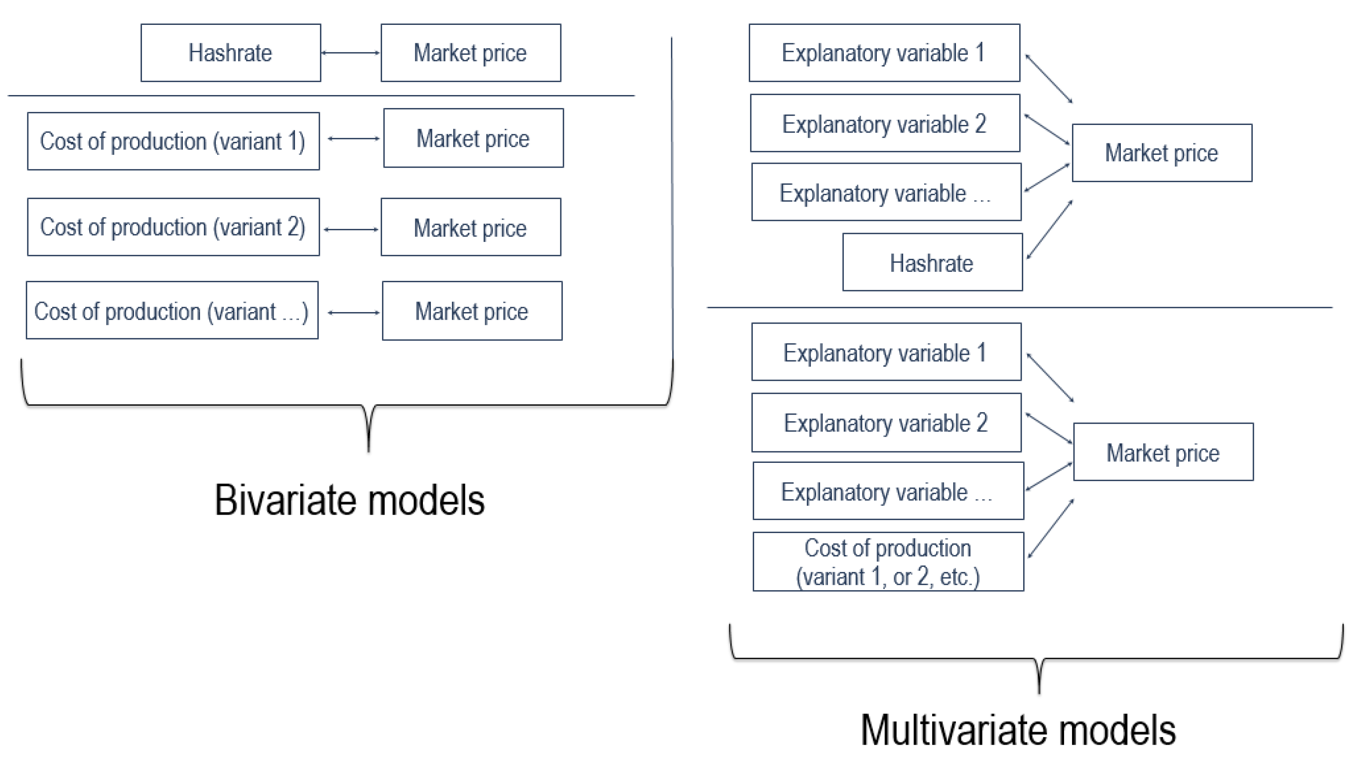
Figure 2.
Energy efficiency of ASIC data scraped from the “Mining hardware comparison” webpage, and the network energy efficiency reported by Hayes (2019). Logarithmic scale.

Figure 3.
Energy efficiency curves estimated with models 1 and 2 in (4) for the whole Bitcoin network, and the respective ASIC releases. The reported data are measured in Joule/Giga-Hash.
Figure 3.
Energy efficiency curves estimated with models 1 and 2 in (4) for the whole Bitcoin network, and the respective ASIC releases. The reported data are measured in Joule/Giga-Hash.
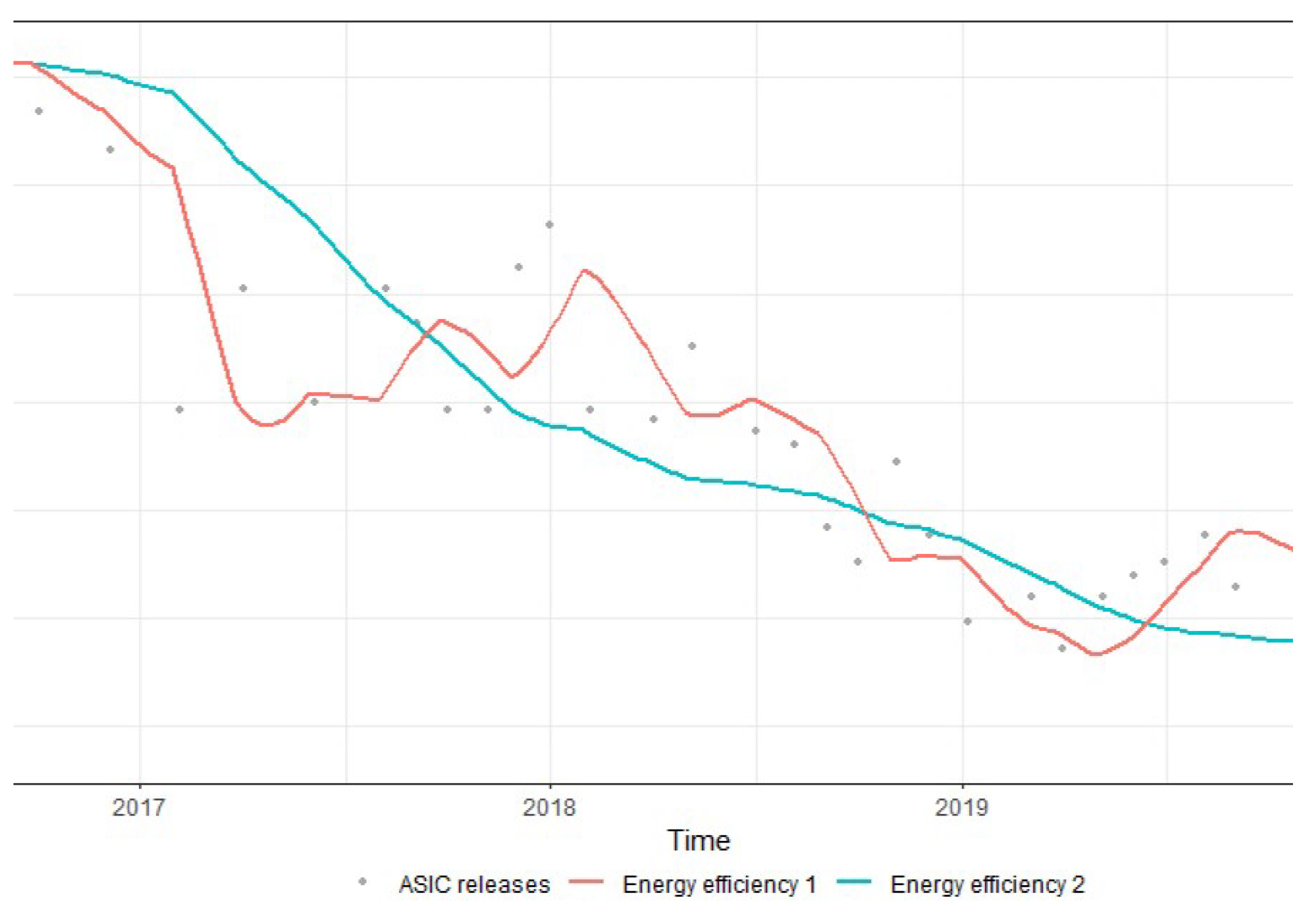
Figure 4.
A sudden jump can be seen just before August 2016, highlighting the drawback of cost of production model. Logarithmic scale.
Figure 4.
A sudden jump can be seen just before August 2016, highlighting the drawback of cost of production model. Logarithmic scale.

Figure 5.
Variables used in the analysis.
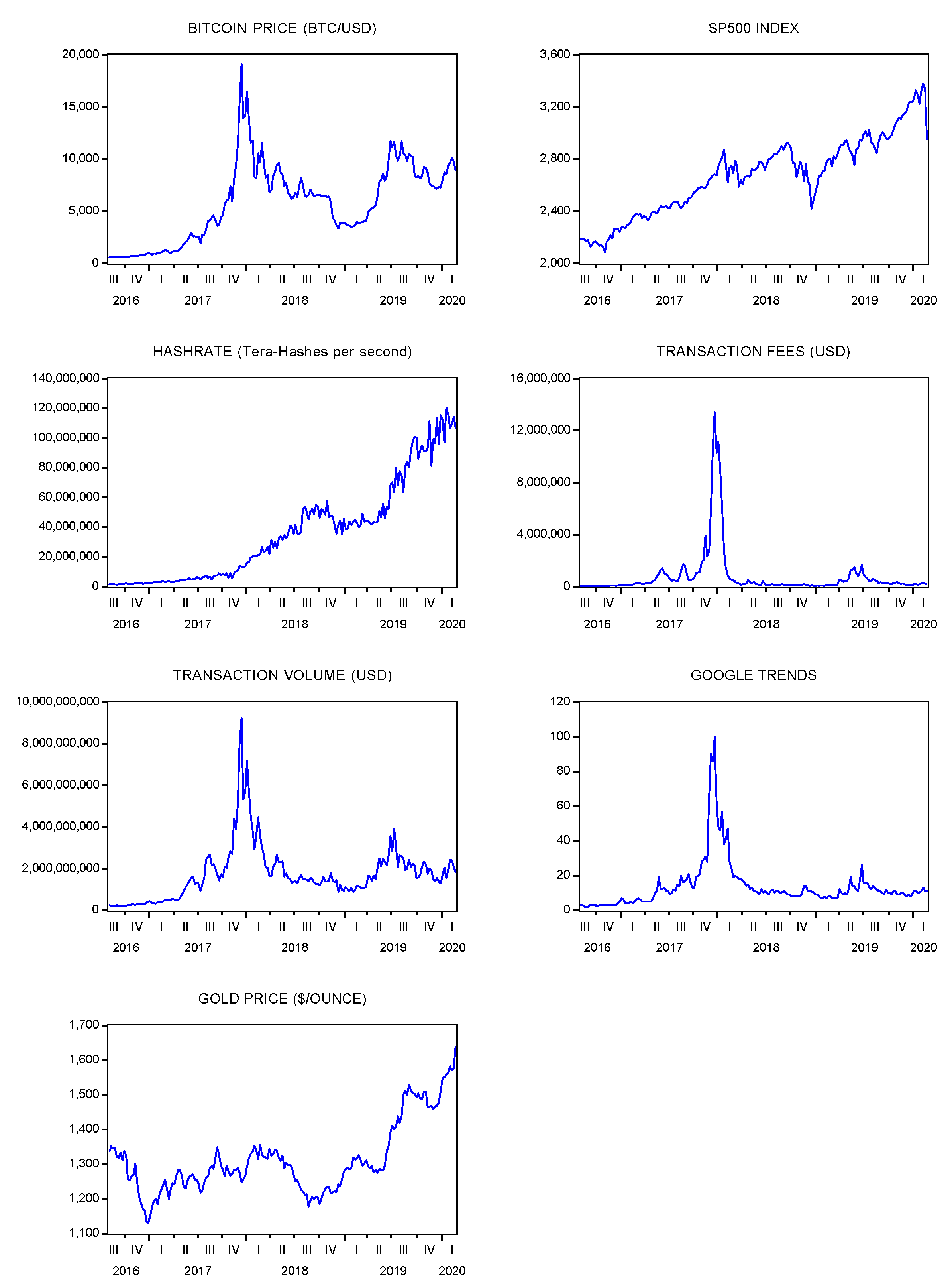
Figure 6.
Cost-of-production model prices: Model 1 and Model 2 from Equation (4).
Figure 6.
Cost-of-production model prices: Model 1 and Model 2 from Equation (4).
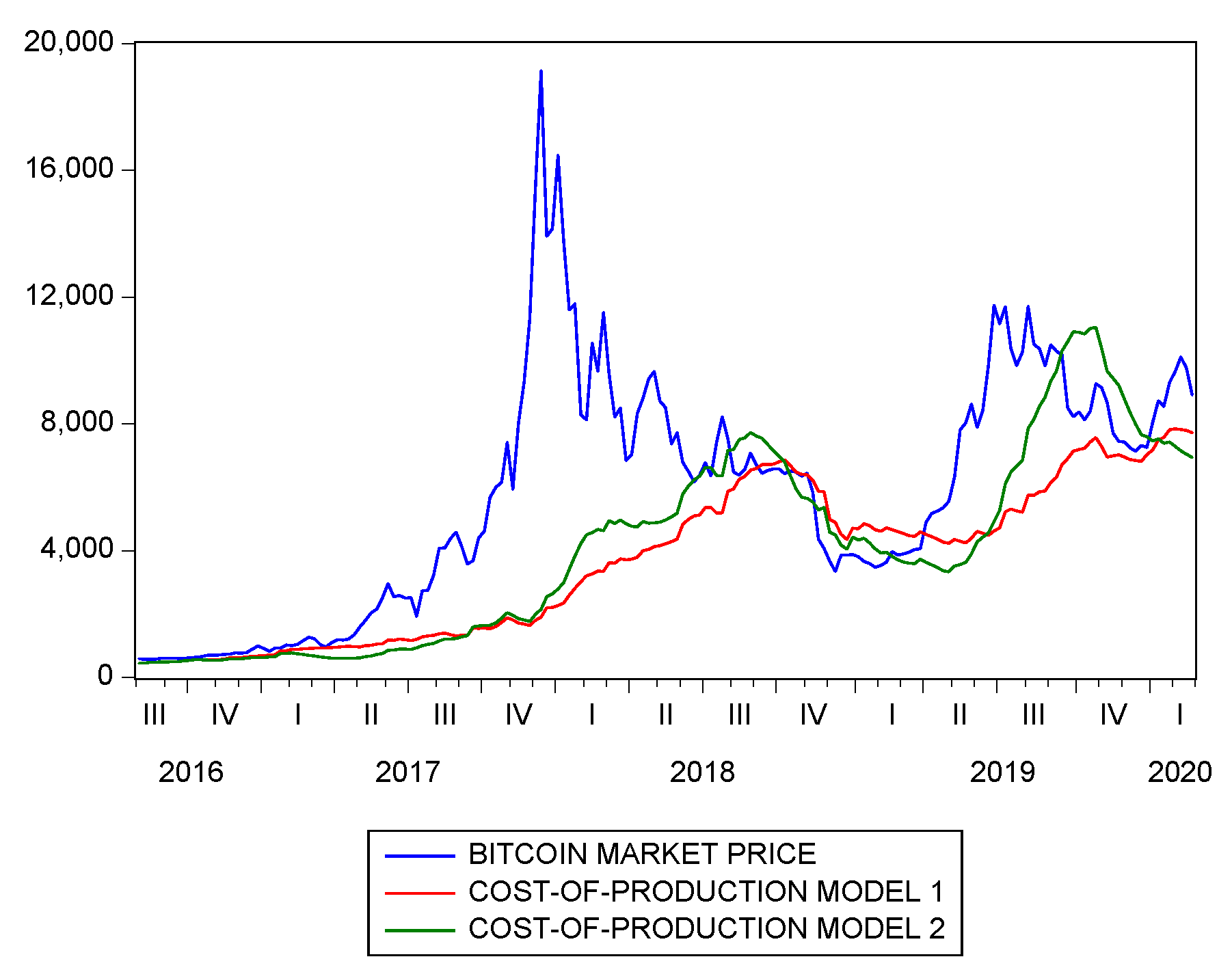
Figure 7.
Nord Pool system price and the fixed electricity price of 0.13 $/kWh.

Figure 8.
Bitcoin cost-of-production prices computed using both constant electricity prices and Nord Pool prices, together with the bitcoin market price.
Figure 8.
Bitcoin cost-of-production prices computed using both constant electricity prices and Nord Pool prices, together with the bitcoin market price.
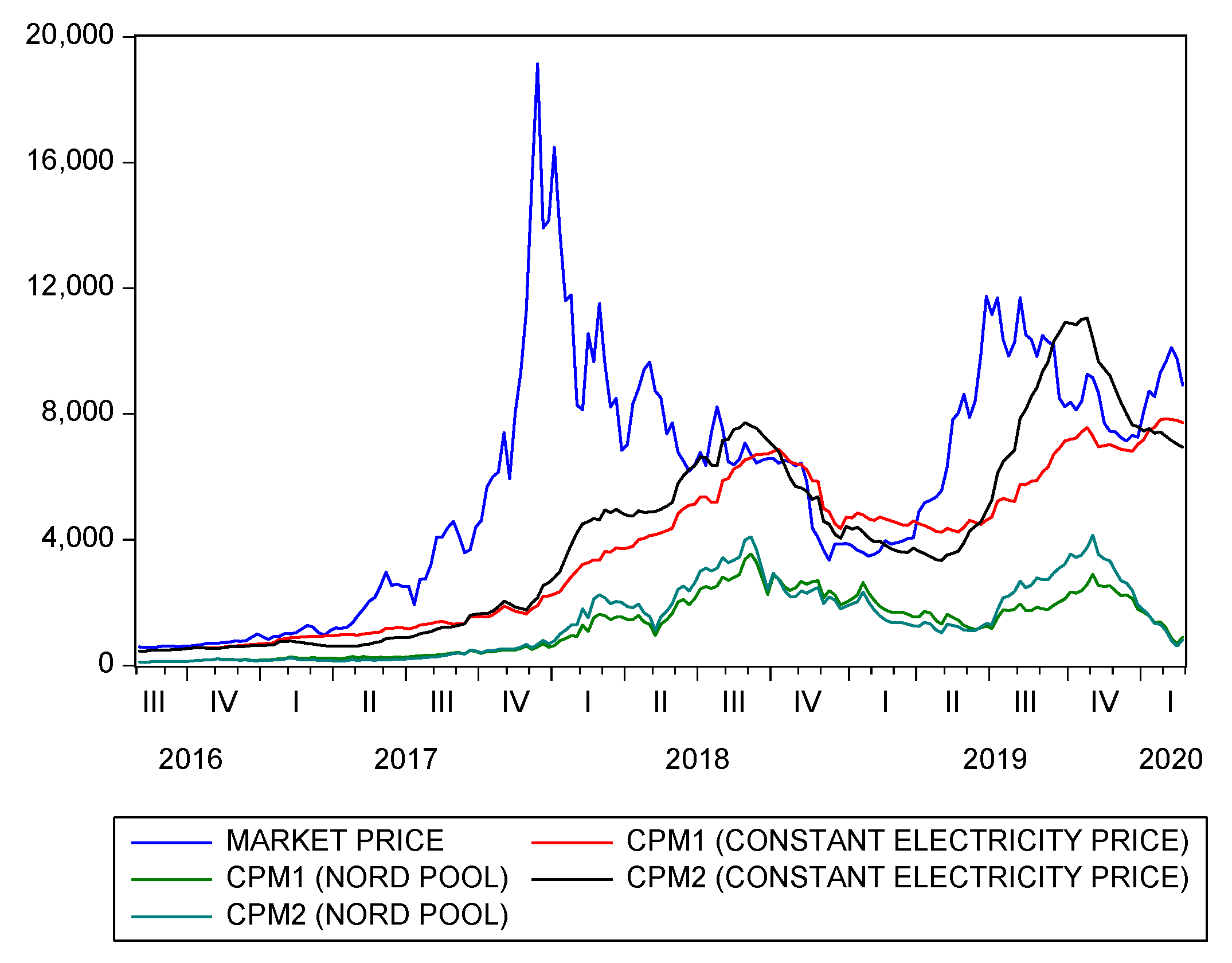
Table 1.
Description of the explanatory variables used in the analysis.
| Variable | Description | Source |
|---|---|---|
| Bitcoin price (USD) | Coinmarketcap computes an average price weighted by the trade volume of the exchanges that offer bitcoin trading pairs. | Coinmarketcap.com |
| Hashrate | It is measured in tera-hashes per second (one hash is equal to a double SHA-256 computation) | Coinmetrics.io |
| Transaction fees (USD) | This is the total amount of money paid by the users for the service of moving their funds. It is computed as the weekly average of the total daily transaction fees in bitcoin multiplied with the weekly average of the bitcoin price. | Coinmetrics.io |
| Transaction volume (USD) | This is the total value transacted on the Bitcoin network multiplied with the weekly average of the bitcoin price. | Coinmetrics.io |
| Google Trends | Weekly search data for the word “bitcoin” worldwide | trends.google.com |
| Gold Price ($/Ounce) | Price in USD per troy ounce as reported by the London Bullion Market Association. Gold is often compared with bitcoin, and the reported similarities include: limited supply, low correlation with stock markets, and its main use as store of value rather than unit of account. | Quandl.com |
| SP500 | This index is taken as an indicator of the general public perception of the global markets. We assume public optimism towards investment to play a certain role in the demand for bitcoin. | Yahoo Finance |
Table 2.
Unit root tests. Null hypothesis: the time series has a unit root. * Significant at the 5% level.
Table 2.
Unit root tests. Null hypothesis: the time series has a unit root. * Significant at the 5% level.
| Vogelsang and Perron (1998) | Lee and Strazicich (2003) | |||
|---|---|---|---|---|
| Variable | t-Statistic | Break Date | t-Statistic | Break Date |
| Log(Bitcoin price) | −3.43 | 20/03/2017 | −1.72 | 10/07/2017 |
| Log(Hashrate) | −3.46 | 06/11/2017 | −2.05 | 06/11/2017 |
| Log(Transaction_fees) | −2.69 | 04/12/2017 | −2.56 | 18/06/2018 |
| Log(Transaction_volume) | −3.55 | 17/04/2017 | −2.07 | 24/07/2017 |
| Log(Google) | −3.01 | 24/04/2017 | −2.11 | 15/05/2017 |
| Log(Gold) | −3.14 | 03/06/2019 | −2.59 | 05/08/2019 |
| Log(SP500) | −2.84 | 17/12/2018 | −3.36 | 15/10/2018 |
| DLog(Bitcoin price) | −13.45 * | 04/12/2017 | −7.89 * | 27/11/2017 |
| DLog(Hashrate) | −25.75 * | 30/07/2018 | −4.32 * | 19/11/2018 |
| DLog(Transaction_fees) | −11.68 * | 01/04/2019 | −5.73 * | 27/11/2017 |
| DLog(Transaction_volume) | −15.66 * | 04/12/2017 | −7.71 * | 15/01/2018 |
| DLog(Google) | −15.18 * | 27/11/2017 | −8.45 * | 06/11/2017 |
| DLog(Gold) | −12.61 * | 19/12/2016 | −5.22 * | 16/04/2018 |
| DLog(SP500) | −15.20 * | 17/02/2020 | −8.54 * | 03/12/2018 |
Table 3.
p-values for the Granger causality tests using the Toda and Yamamoto (1995) approach. The tests for the CPM(model 1)-CPM(model 2), CPM(model 1)-Hashrate, and CPM(model 2)-Hashrate pairs were not computed for obvious reasons, given how the CPMs are constructed. p-values smaller than 0.05 are in bold font.
| First Sample: 01/08/2016–04/12/2017 | |||||
|---|---|---|---|---|---|
| Dependent variable (Y) | |||||
| Log(Bitcoin Price) | Log(CPM_model_1) | Log(CPM_model_2) | Log(Hashrate) | ||
| Log(Bitcoin price) | / | 0.92 | 0.66 | 0.82 | |
| Regressor | Log(CPM_model_1) | 0.92 | / | / | / |
| (X) | Log(CPM_model_2) | 0.95 | / | / | / |
| Log(Hashrate) | 0.52 | / | / | / | |
| Second sample: 11/12/2017–24/02/2020 | |||||
| Dependent variable (Y) | |||||
| Log(Bitcoin Price) | Log(CPM_model_1) | Log(CPM_model_2) | Log(Hashrate) | ||
| Log(Bitcoin price) | / | 0.06 | 0.01 | 0.00 | |
| Regressor | Log(CPM_model_1) | 0.90 | / | / | / |
| (X) | Log(CPM_model_2) | 0.33 | / | / | / |
| Log(Hashrate) | 0.10 | / | / | / | |
Table 4.
Bivariate Johansen cointegration tests. The null hypothesis is the absence of cointegration. All the tests considered the case of an intercept in the cointegration equation (CE) only.
Table 4.
Bivariate Johansen cointegration tests. The null hypothesis is the absence of cointegration. All the tests considered the case of an intercept in the cointegration equation (CE) only.
| Bivariate Variable Pair | 01/08/2016–04/12/2017 | 11/12/2017–24/02/2020 |
|---|---|---|
| N. of CEs at 5% Level | N. of CEs at 5% Level | |
| Log(Bitcoin price), Log(CPM_model_1) | 0 | 1 |
| Log(Bitcoin price), Log(CPM_model_2) | 0 | 1 |
| Log(Bitcoin price), Log(Hashrate) | 0 | 1 |
Table 5.
Misspecification tests on the residuals from the bivariate models. p-values smaller than 5% are reported in bold font.
Table 5.
Misspecification tests on the residuals from the bivariate models. p-values smaller than 5% are reported in bold font.
| First Sample: 01/08/2016–04/12/2017 | |||
|---|---|---|---|
| Bivariate variable pair: | Bivariate variable pair: | Bivariate variable pair: | |
| Log(Bitcoin price), | Log(Bitcoin price), | Log(Bitcoin price), | |
| Log(CPM_model_1) | Log(CPM_model_2) | Log(Hashrate) | |
| Model selected | VAR(0) for Log-returns | VAR(0) for Log-returns | VAR(1) for Log-returns |
| Multivariate LM test (lag 4) | 0.33 | 0.59 | 0.45 |
| Multivariate LM test (lag 8) | 0.87 | 0.85 | 0.26 |
| Multivariate LM test (lag 12) | 0.45 | 0.64 | 0.60 |
| Multivariate White test | 0.00 | 0.08 | 0.00 |
| Multivariate Normality test | 0.00 | 0.00 | 0.58 |
| BDS (dim = 6) residuals 1st eq. | 0.16 | 0.16 | 0.47 |
| BDS (dim = 6) residuals 2nd eq. | 0.48 | 0.31 | 0.50 |
| Is bitcoin price weakly exogenous? | Yes | Yes | Yes (short-run: p value = 0.29) |
| Second sample: 11/12/2017–24/02/2020 | |||
| Bivariate variable pair: | Bivariate variable pair: | Bivariate variable pair: | |
| Log(Bitcoin price), | Log(Bitcoin price), | Log(Bitcoin price), | |
| Log(CPM_model_1) | Log(CPM_model_2) | Log(Hashrate) | |
| Model selected | VECM(0) | VECM(2) | VECM(6) |
| Multivariate LM test (lag 4) | 0.08 | 0.15 | 0.20 |
| Multivariate LM test (lag 8) | 0.44 | 0.21 | 0.36 |
| Multivariate LM test (lag 12) | 0.64 | 0.54 | 0.91 |
| Multivariate White test | 0.00 | 0.00 | 0.07 |
| Multivariate Normality test | 0.00 | 0.00 | 0.58 |
| BDS (dim = 6) residuals 1st eq. | 0.00 | 0.00 | 0.02 |
| BDS (dim = 6) residuals 2nd eq. | 0.02 | 0.85 | 0.88 |
| Is bitcoin price weakly exogenous? | Yes (long-run: p value = 0.08) | Yes (long-run: pvalue = 0.37) | Yes (long-run: p value = 0.06) |
| (short-run: p value = 0.97) | (short-run: p value = 0.07) | ||
Table 6.
Weak exogeneity tests: variables for which the null hypothesis of weak exogeneity can be rejected after re-testing at the 5% probability level.
Table 6.
Weak exogeneity tests: variables for which the null hypothesis of weak exogeneity can be rejected after re-testing at the 5% probability level.
| First Sample: 01/08/2016–04/12/2017 | |||||
|---|---|---|---|---|---|
| Log(Transaction Fees) | Log(Transaction Volume) | Log(Hashrate) | Log(SP500) | Log(GOLD) | Log(Google) |
| V | |||||
| Log(Transaction Fees) | Log(Transaction Volume) | Log(CPM_model_1) | Log(SP500) | Log(GOLD) | Log(Google) |
| V | |||||
| Log(Transaction Fees) | Log(Transaction Volume) | Log(CPM_model_2) | Log(SP500) | Log(GOLD) | Log(Google) |
| V | |||||
| Second Sample: 11/12/2017–24/02/2020 | |||||
| Log(Transaction Fees) | Log(Transaction Volume) | Log(Hashrate) | Log(SP500) | Log(GOLD) | Log(Google) |
| V | |||||
| Log(Transaction Fees) | Log(Transaction Volume) | Log(CPM_model_1) | Log(SP500) | Log(GOLD) | Log(Google) |
| V | V | ||||
| Log(Transaction Fees) | Log(Transaction Volume) | Log(CPM_model_2) | Log(SP500) | Log(GOLD) | Log(Google) |
| V | |||||
Table 7.
Multivariate Johansen cointegration tests. The null hypothesis is the absence of cointegration. The tests considered either the case of an intercept in the cointegration equation (CE) and a trend in the variables (first sample) or the case of an intercept in the CE only (second sample). (*) The final model turned out to be the same, independently of whether we used the hashrate, or the CPM1, or the CPM2.
| First Sample: | 01/08/2016-04/12/2017 |
|---|---|
| Variables | N. of CEs at 5% level |
| Log(Bitcoin_price), Log(Google) (*) | 1 |
| Log(Bitcoin_price), Log(Google) (*) | 1 |
| Log(Bitcoin_price), Log(Google) (*) | 1 |
| Second sample: | 11/12/2017-24/02/2020 |
| Variables | N. of CEs at 5% level |
| Log(Bitcoin_price), Log(Hashrate) | 1 |
| Log(Bitcoin_price), Log(CPM_model_1), Log(Transaction volume) | 1 |
| Log(Bitcoin_price), Log(CPM_model_2) | 1 |
Table 8.
Misspecification tests on the residuals from the multivariate models. p-values smaller than 5% are reported in bold font. (*) The final model turned out to be the same, independently of whether we used the hashrate, or the CPM1, or the CPM2.
Table 8.
Misspecification tests on the residuals from the multivariate models. p-values smaller than 5% are reported in bold font. (*) The final model turned out to be the same, independently of whether we used the hashrate, or the CPM1, or the CPM2.
| First Sample: 01/08/2016–04/12/2017 | |||
|---|---|---|---|
| Variables: | Variables: | Variables: | |
| Log(Bitcoin_price), | Log(Bitcoin_price), | Log(Bitcoin_price), | |
| Log(Google) | Log(Google) | Log(Google) | |
| (*) | (*) | (*) | |
| Model selected | VECMX(1) | VECMX(1) | VECMX(1) |
| Multivariate LM test (lag 4) | 0.99 | 0.99 | 0.99 |
| Multivariate LM test (lag 8) | 0.88 | 0.88 | 0.88 |
| Multivariate LM test (lag 12) | 0.45 | 0.45 | 0.45 |
| Multivariate White test | 0.10 | 0.10 | 0.10 |
| Multivariate Normality test | 0.00 | 0.00 | 0.00 |
| BDS (dim = 6) residuals 1st eq. | 0.73 | 0.73 | 0.73 |
| BDS (dim = 6) residuals 2nd eq. | 0.28 | 0.28 | 0.28 |
| Is bitcoin price weakly exogenous? | Yes (long-run: p value = 0.72) | Yes (long-run: p value = 0.72) | Yes (long-run: p value = 0.72) |
| (short-run: p value = 0.83) | (short-run: p value = 0.83) | (short-run: p value = 0.83) | |
| Second sample: 11/12/2017–24/02/2020 | |||
| Variables: | Variables: | Variables: | |
| Log(Bitcoin_price), | Log(Bitcoin_price), | Log(Bitcoin_price), | |
| Log(Hashrate) | Log(CPM_model_1) | Log(CPM_model_2) | |
| Log(Transaction volume) | |||
| Model selected | VECMX(6) | VECMX(2) | VECMX(2) |
| Multivariate LM test (lag 4) | 0.58 | 0.34 | 0.68 |
| Multivariate LM test (lag 8) | 0.21 | 0.59 | 0.18 |
| Multivariate LM test (lag 12) | 0.99 | 0.73 | 0.28 |
| Multivariate White test | 0.40 | 0.00 | 0.04 |
| Multivariate Normality test | 0.93 | 0.03 | 0.00 |
| BDS (dim = 6) residuals 1st eq. | 0.01 | 0.05 | 0.03 |
| BDS (dim = 6) residuals 2nd eq. | 0.70 | 0.01 | 0.66 |
| BDS (dim = 6) residuals 3rd eq. | / | 0.01 | / |
| Is bitcoin price weakly exogenous? | Yes (long-run: p value = 0.60) | Yes (long-run: p value = 0.86) | Yes (long-run: p value = 0.88) |
| (short-run: p value = 0.09) | (short-run: p value = 0.81) | (short-run: p value = 0.07) | |
Publisher’s Note: MDPI stays neutral with regard to jurisdictional claims in published maps and institutional affiliations. |
© 2020 by the authors. Licensee MDPI, Basel, Switzerland. This article is an open access article distributed under the terms and conditions of the Creative Commons Attribution (CC BY) license (http://creativecommons.org/licenses/by/4.0/).
Share and Cite
MDPI and ACS Style
Fantazzini, D.; Kolodin, N. Does the Hashrate Affect the Bitcoin Price? J. Risk Financial Manag. 2020, 13, 263. https://doi.org/10.3390/jrfm13110263
AMA Style
Fantazzini D, Kolodin N. Does the Hashrate Affect the Bitcoin Price? Journal of Risk and Financial Management. 2020; 13(11):263. https://doi.org/10.3390/jrfm13110263
Chicago/Turabian StyleFantazzini, Dean, and Nikita Kolodin. 2020. "Does the Hashrate Affect the Bitcoin Price?" Journal of Risk and Financial Management 13, no. 11: 263. https://doi.org/10.3390/jrfm13110263