Role of Meteorological Parameters in the Diurnal and Seasonal Variation of NO2 in a Romanian Urban Environment

 , ,
, ,  ,
,
Abstract
:1. Introduction
2. Data and Methods/Experimental
2.1. Data
2.2. Methods
3. Results and Discussion
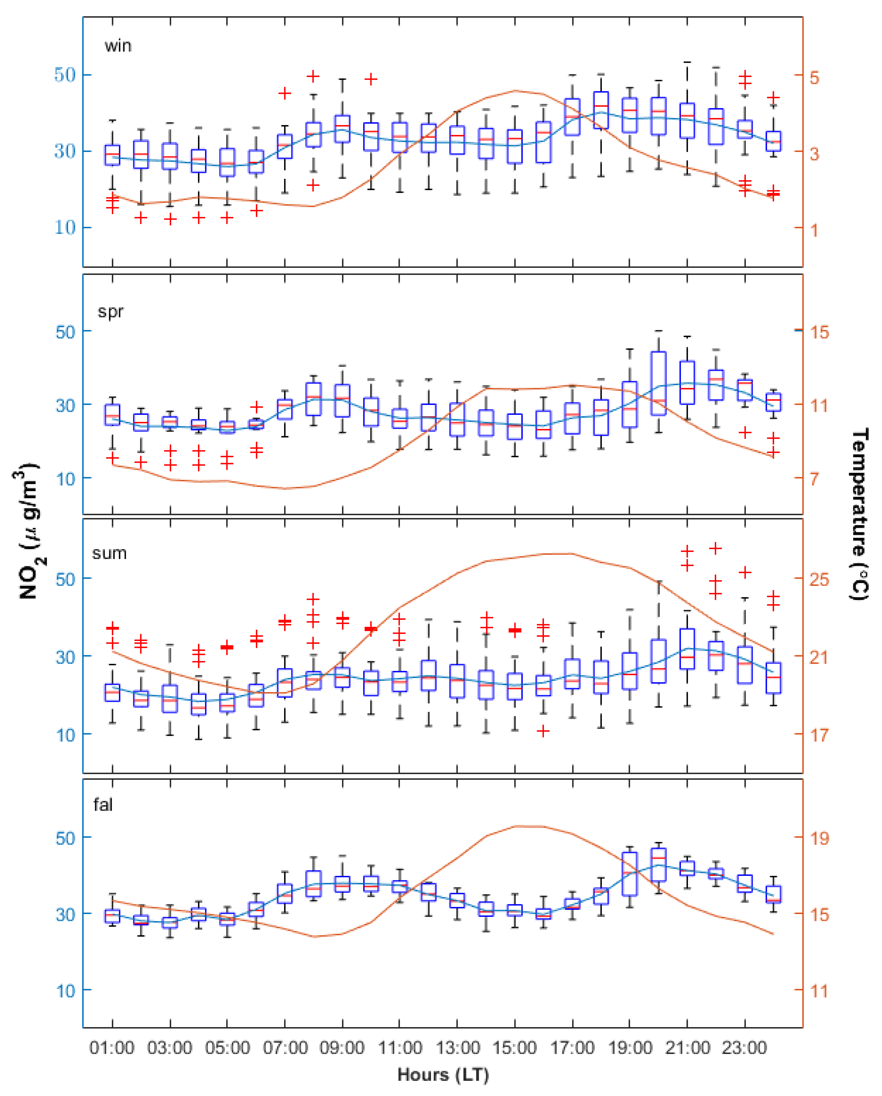
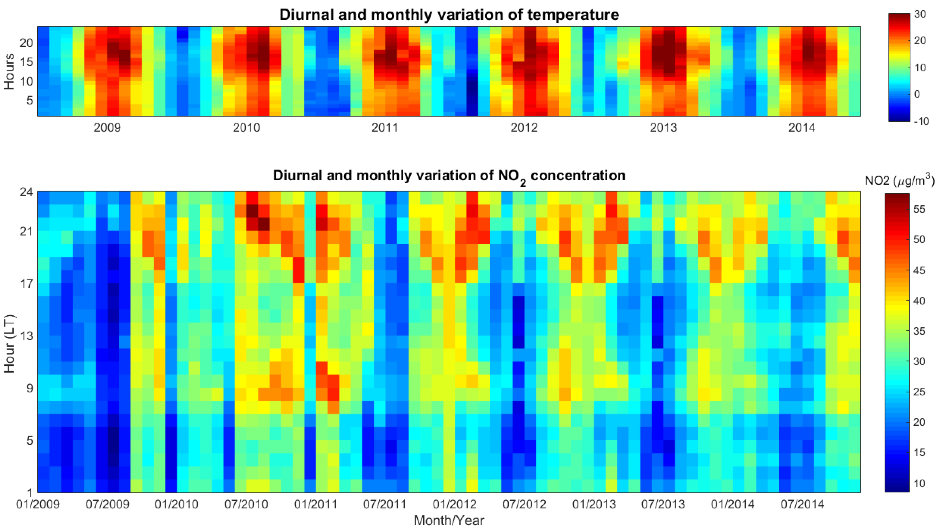
3.1. Diurnal and Seasonal Variation
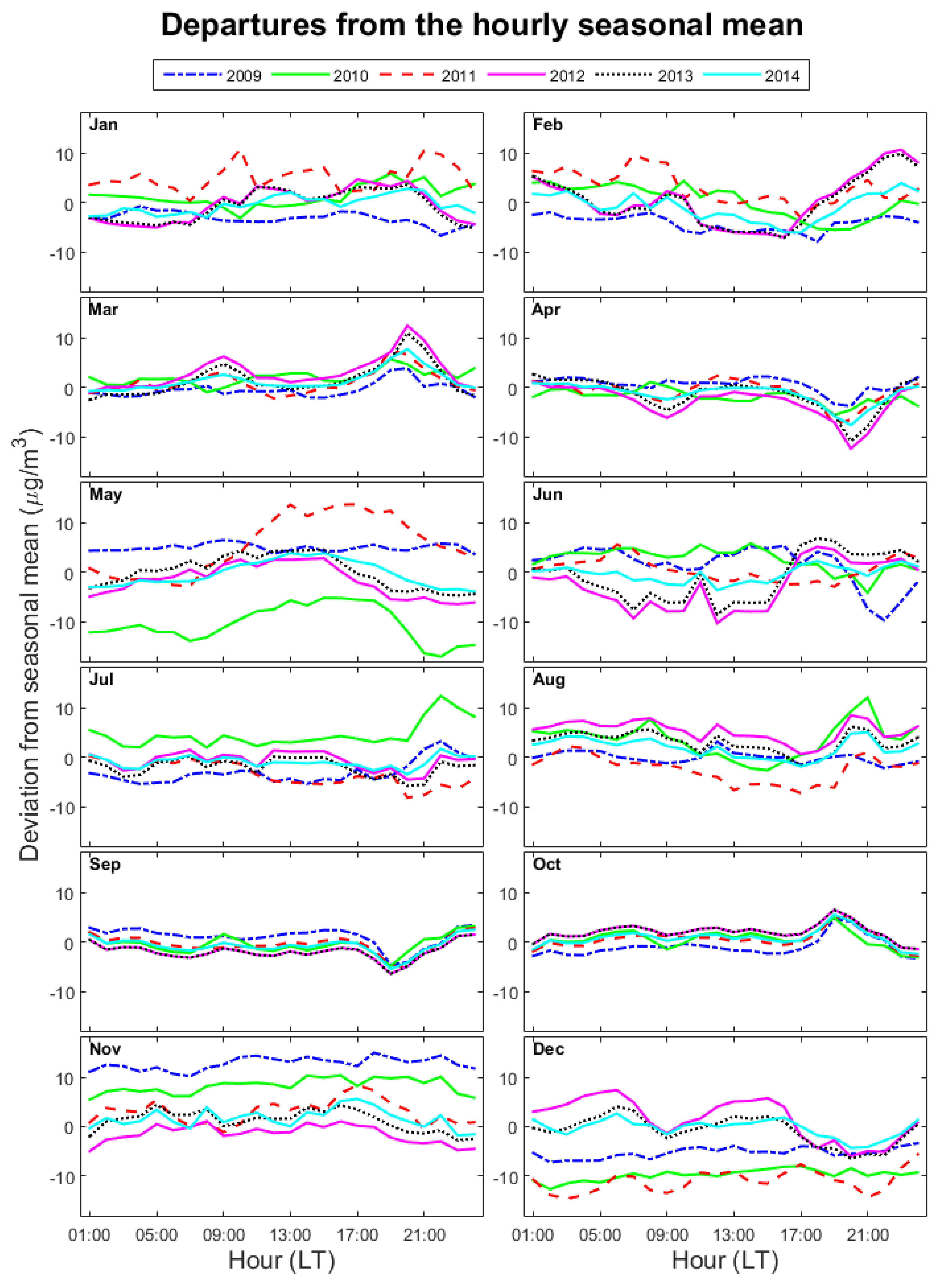
3.2. Monthly Deviation of NO2 Concentration from the Seasonal Mean
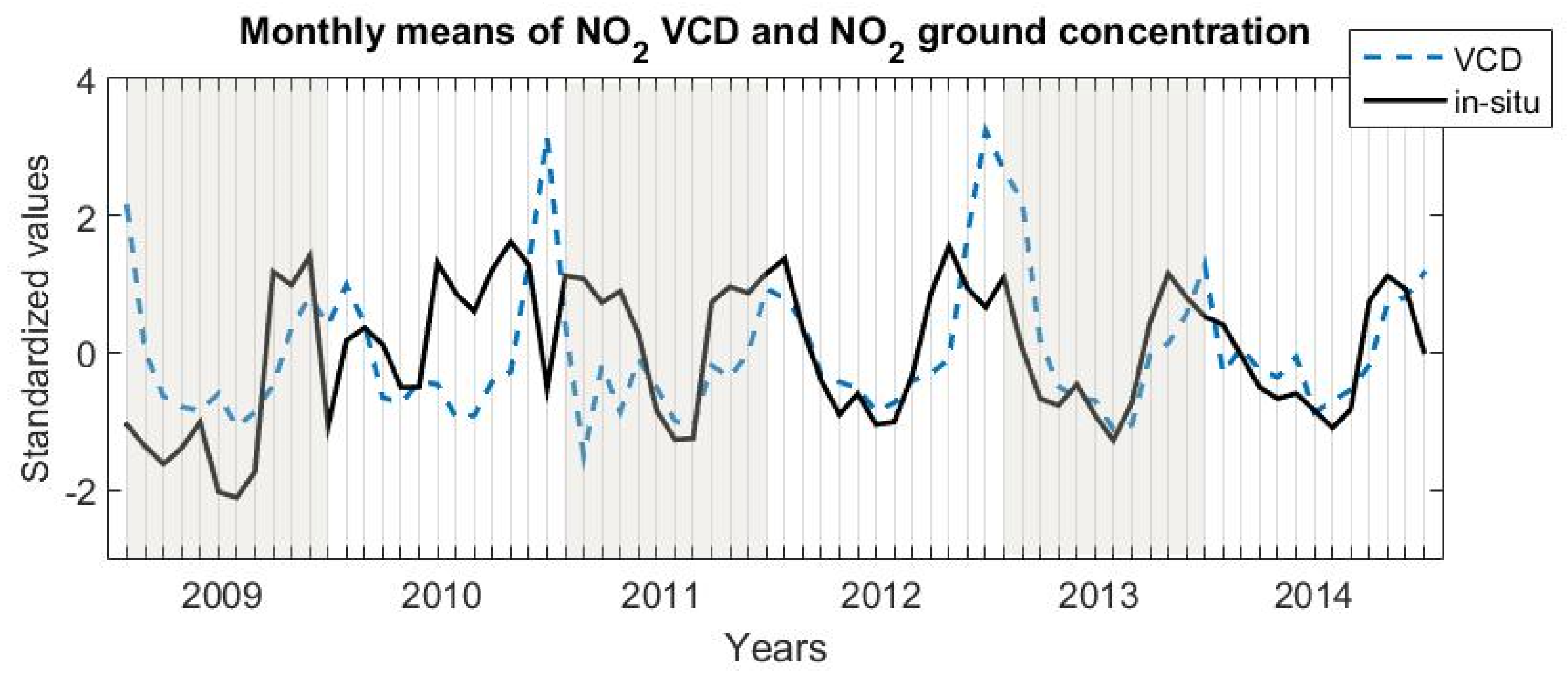
3.3. Correlation between NO2 Concentration and Meteorological Parameters
4. Conclusions
Author Contributions
Funding
Acknowledgments
Conflicts of Interest
References
- Schaube, D.; Brunner, D.; Boersma, K.F.; Keller, J.; Folini, D.; Buchmann, B.; Berresheim, H.; Staehelin, J. SCIAMACHY tropospheric NO2 over Switzerland: Estimates of NOx lifetimes and impact of the complex Alpine topography on the retrieval. Atmos. Chem. Phys. 2007, 7, 5971–5987. [Google Scholar] [CrossRef] [Green Version]
- Air Quality Expert Group. Nitrogen Dioxide in the United Kingdom: Summary, prepared for The Department for Environment, Food and Rural Affairs; Scottish Executive: Edinburgh, UK; Welsh Assembly Government: Cardiff, UK; Department of the Environment in Northern Ireland: Belfast, UK, 2004. [Google Scholar]
- Schumann, U.; Huntrieser, H. The global lightning-induced nitrogen oxides source. Atmos. Chem. Phys. 2007, 7, 3823. [Google Scholar]
- Stavrakou, T.; Müller, J.-F.; Boersma, K.F.; van der AR, J.; Kurokawa, J.; Ohara, T.; Zhang, Q. Key chemical NOx sink uncertainties and how they influence top-down emissions of nitrogen oxides. Atmos. Chem. Phys. 2013, 13, 9057–9082. [Google Scholar]
- Çelik, M.; Kadi, I. The Relation Between Meteorological Factors and Pollutants Concentrations in Karabük City. Gazi Univ. J. Sci. 2007, 20, 87–95. [Google Scholar]
- Dunlea, E.J.; Herndon, S.C.; Nelson, D.D.; Volkamer, R.M.; San Martini, F.; Sheehy, P.M.; Zahniser, M.S.; Shorter, J.H.; Wormhoudt, J.C.; Lamb, B.K.; et al. Evaluation of nitrogen dioxide chemiluminescence monitors in a polluted urban environment. Atmos. Chem. Phys. 2007, 20, 2691–2704. [Google Scholar]
- Kendrick, C.M.; Koonce, P.; George, L.A. Diurnal and seasonal variations of NO, NO2 and PM2.5 mass as a function of traffic volumes alongside an urban arterial. Atmos. Environ. 2015, 122, 133–141. [Google Scholar]
- Dragomir, D.; Constantin, D.; Voiculescu, M.; Georgescu, L.; Merlaud, A.; Roozendael, M. Modeling results of atmospheric dispersion of NO2 in an urban area using METI–LIS and comparison with coincident mobile DOAS measurements. Atmos. Poll. Res. 2015, 6, 503–510. [Google Scholar]
- Cichowicz, R.; Wielgosiński, G.; Fetter, W. Dispersion of atmospheric air pollution in summer and winter season. Environ. Monit. Assess. 2017, 189, 605. [Google Scholar]
- Degraeuwe, B.; Thunis, P.; Clappier, A.; Weiss, M.; Lefebvre, W.; Janssen, S.; Vranckx, S. Impact of passenger car NOx emissions and NO2 fractions on urban, NO2 pollution e Scenario analysis for the city of Antwerp, Belgium. Atm. Environ. 2017, 126, 218–224. [Google Scholar]
- Casquero-Vera, J.-A.; Lyamani, H.; Titos, G.; Borrás, E.; Olmo, F.; Allados-Arboledas, L. Impact of primary NO2 emissions at different urban sites exceeding the European NO2 standard limit. Sci. Total Environ. 2019, 646, 1117–1125. [Google Scholar] [CrossRef]
- Parrish, D.D. Critical evaluation of US on-road vehicle emission inventories. Atmos. Environ. 2006, 40, 2288–2300. [Google Scholar]
- Elminir, H.K. Dependence of urban air pollutants on meteorology. Sci. Total Environ. 2005, 350, 225–237. [Google Scholar]
- Verma, S.; Desai, B. Effect of Meteorological Conditions on Air Pollution of Surat City. J. Int. Environ. Appl. Sci. 2008, 3, 358–367. [Google Scholar]
- Dominick, D.; Latif, M.; Juahir, H.; Aris, A.; Zain, S. An assessment of influence of meteorological factors on PM10 and NO2 at selected stations in Malaysia. Sustain. Environ. Res. 2012, 22, 305–315. [Google Scholar]
- Hosseinibalam, F.; Hejazi, A. Influence of Meteorological Parameters on Air Pollution in Isfahan. Int. Proc. Chem. Biol. Environ. Eng. 2012, 46, 7–12. [Google Scholar]
- Srivastava, R.; Sarkar, S.; Beig, G. Correlation of Various Gaseous Pollutants with Meteorological Parameter (Temperature, Relative Humidity and Rainfall). Glob. J. Sci. Front. Res. Environ. Earth Sci. 2014, 14, 57–65. [Google Scholar]
- Habeebullah, T.M.; Munir, S.; Awad, A.H.A.; Morsy, E.A.; Seroji, A.R.; Mohammed, A.M.F. The Interaction between Air Quality and Meteorological Factors in an Arid Environment of Makkah, Saudi Arabia. Int. J. Environ. Sci. Dev. 2015, 6, 576–580. [Google Scholar] [CrossRef] [Green Version]
- Zhang, H.; Wang, Y.; Hu, J.; Ying, Q.; Hu, X.-M. Relationships between meteorological parameters and criteria air pollutants in three megacities in China. Environ. Res. 2015, 140, 242–254. [Google Scholar] [CrossRef]
- Gasmi, K.; Aljalal, A.; Al-Basheer, W.; Abdulahi, M. Analysis of NOx, NO and NO2 Ambient Levels as a Function of Meteorological Parameters in Dhahran, Saudi Arabia. Air Pollut. XXV 2017, 1, 77–86. [Google Scholar] [CrossRef] [Green Version]
- Nascu, H.I.; Jantschi, L. Analytical and Instrumental Chemistry, Cluj-Napoca; Academic Press & Academic Direct: Cambridge, MA, USA, 2006; pp. 170–172. [Google Scholar]
- Levelt, P.; Oord, G.V.D.; Dobber, M.; Malkki, A.; Visser, H.; De Vries, J.; Stammes, P.; Lundell, J.; Saari, H. The ozone monitoring instrument. IEEE Trans. Geosci. Remote Sens. 2006, 44, 1093–1101. [Google Scholar] [CrossRef]
- Bucsela, E.; Celarier, E.; Wenig, M.; Gleason, J.; Veefkind, J.; Boersma, F.; Brinksma, E. Algorithm for NO/sub 2/ vertical column retrieval from the ozone monitoring instrument. IEEE Trans. Geosci. Remote Sens. 2006, 44, 1245–1258. [Google Scholar] [CrossRef]
- Duncan, B.N.; Geigert, M.; Lamsal, L. A Brief Tutorial on Using the Ozone Monitoring Instrument (OMI) Nitrogen Dioxide (NO2) Data Product for SIPS Preparation. HAQAST Tech. Guid. Doc. 2018. [Google Scholar] [CrossRef]
- Lamsal, L.N.; Martin, R.V.; Van Donkelaar, A.; Steinbächer, M.; Celarier, E.A.; Bucsela, E.; Dunlea, E.J.; Pinto, J.P. Ground-level nitrogen dioxide concentrations inferred from the satellite-borne Ozone Monitoring Instrument. J. Geophys. Res. Space Phys. 2008, 113, 1–15. [Google Scholar] [CrossRef] [Green Version]
- Boersma, F.; Jacob, D.J.; Trainic, M.; Rudich, Y.; Desmedt, I.; Dirksen, R.; Eskes, H.J. Validation of urban NO2 concentrations and their diurnal and seasonal variations observed from the SCIAMACHY and OMI sensors using in situ surface measurements in Israeli cities. Atmos. Chem. Phys. Discuss. 2009, 9, 3867–3879. [Google Scholar] [CrossRef] [Green Version]
- Gruzdev, A.N.; Elokhov, A.S. Validation of Ozone Monitoring Instrument NO2 measurements using ground based NO2 measurements at Zvenigorod, Russia. Int. J. Remote. Sens. 2010, 31, 497–511. [Google Scholar] [CrossRef]
- Constantin, D.-E.; Voiculescu, M.; Georgescu, L.P. Satellite Observations of NO2 Trend over Romania. Sci. World J. 2013, 2013, 261634. [Google Scholar] [CrossRef]
- Lee, H.J.; Koutrakis, P. Daily Ambient NO2 Concentration Predictions Using Satellite Ozone Monitoring Instrument NO2 Data and Land Use Regression. Environ. Sci. Technol. 2014, 48. [Google Scholar] [CrossRef]
- Krotkov, N.A.; McLinden, C.A.; Li, C.; Lamsal, L.N.; Celarier, E.A.; Marchenko, S.V.; Swartz, W.H.; Bucsela, E.J.; Joiner, J.; Duncan, B.N.; et al. Aura OMI observations of regional SO2 and NO2 pollution changes from 2005 to 2015. Atmos. Chem. Phys. Discuss. 2016, 16, 4605–4629. [Google Scholar] [CrossRef] [Green Version]
- Anand, J.S.; Monks, P.S. Estimating daily surface NO2 concentrations from satellite data – a case study over Hong Kong using land use regression models. Atmos. Chem. Phys. 2017, 17, 8211–8230. [Google Scholar]
- Paraschiv, S.; Constantin, D.E.; Paraschiv, S.L.; Voiculescu, M. OMI and Ground-Based In-Situ Tropospheric Nitrogen Dioxide Observations over Several Important European Cities during 2005–2014. Int. J. Environ. Res. Public Health 2017, 14, 1415. [Google Scholar] [CrossRef] [Green Version]
- Krotkov, N.A. OMI/Aura NO2 Cloud-Screened Total and Tropospheric Column L3 Global Gridded 0.25° × 0.25° V3, NASA Goddard Space Flight Center, Goddard Earth Sciences Data and Information Services Center (GES DISC). Available online: https://disc.gsfc.nasa.gov/datacollection/OMNO2_CPR_003.html (accessed on 25 July 2019).
- Usoskin, I.; Voiculescu, M.; Kovaltsov, G.; Mursula, K. Correlation between clouds at different altitudes and solar activity: Fact or Artifact? J. Atmos. Solar-Terrestrial Phys. 2006, 68, 2164–2172. [Google Scholar] [CrossRef]
- Johnson, R.A.; Bhattacharyya, G.K. Statistics: Principles and Methods, 6th ed.; John Wiley & Sons, Inc.: Hoboken, NJ, USA, 2009; pp. 93–98. [Google Scholar]
- Rosu, A.; Constantin, D.E.; Bocaneala, C.; Arseni, M.; Georgescu, L.P. Evolution of NO2 in five major cities in Europe using remote satellite observations and in situ measurements. In Annals of “Dunarea De Jos” University of Galati Mathematics, Physics, Theoretical Mechanics; Ghent University: Ghent, Belgium, 2016; pp. 66–70. ISSN 20672071. [Google Scholar]
- Constantin, D.E.; Merlaud, A.; Voiculescu, M.; Van Roozendael, M.; Arseni, M.; Rosu, A.; Georgescu, L. NO2 and SO2 observations in SouthEast Europe using mobile DOAS observations. Carpath. J. Earth. Environ. 2017, 12, 323–328. [Google Scholar]
- Wang, S.; Xing, J.; Chatani, S.; Hao, J.; Klimont, Z.; Cofala, J.; Amann, M. Verification of anthropogenic emissions of China by satellite and ground observations. Atmos. Environ. 2011, 45, 6347–6358. [Google Scholar] [CrossRef]
- S.C. TQ Consultanta & Recrutare, S.R.L. The 2014–2020 Urban Strategy of Durable Development of Braila Town; S.C. TQ Consultanta & Recrutare, S.R.L.: Galati, Romania, 2014; pp. 121–132. (in Romanian) [Google Scholar]
- Rosu, A.; Rosu, B.; Arseni, M.; Constantin, D.E.; Voiculescu, M.; Georgescu, L.P.; Van Roozendael, M. Tropospheric nitrogen dioxide measurements in South-East of Romania using zenith-sky mobile DOAS observations. New Technol. Prod. Mach. Manuf. Technol. 2017, 44, 189–194. [Google Scholar]
- Rosu, A.; Rosu, B.; Constantin, D.E.; Voiculescu, M.; Arseni, M.; Murariu, G.; Georgescu, L.P. Correlations between NO2 distribution maps using GIS and mobile DOAS measurements in Galati city. In Annals of “Dunarea de Jos” University of Galati Mathematics, Physics, Theoretical Mechanics; Special Issue; Universitatea “Dunărea de Jos” din Galați: Galati, Romania, 2018; pp. 23–31. ISSN 2067207. [Google Scholar]
- Rosu, A.; Constantin, D.; Rosu, B.; Calmuc, V.; Arseni, M.; Voiculescu, M.; Georgescu, L.P. Mobile measurements of nitrogen dioxide using two different UV-Vis spectrometers. Tech. J. New Technol. Prod. Mach. Manuf. Technol. 2019, 26, 71–76. [Google Scholar]
- Platt, U.; Stutz, J. Differential Absorption Spectroscopy. In Physics of Earth and Space Environments; Springer Science and Business Media LLC: Berlin/Heidelberg, Germany, 2008; pp. 135–174. [Google Scholar]
- Davidson, E.A.; Kingerlee, W. A global inventory of nitric oxide emissions from soils. Nutr. Cycl. Agroecosyst. 1997, 48, 37–50. [Google Scholar] [CrossRef]
- Pancholi, P.; Kumar, A.; Bikundia, D.S.; Chourasiya, S. An observation of seasonal and diurnal behavior of O3 – NOx relationships and local/regional oxidant (OX = O3 + NO2) levels at a semi-arid urban site of western India. Sustain. Environ. Res. 2018, 28, 79–89. [Google Scholar] [CrossRef]


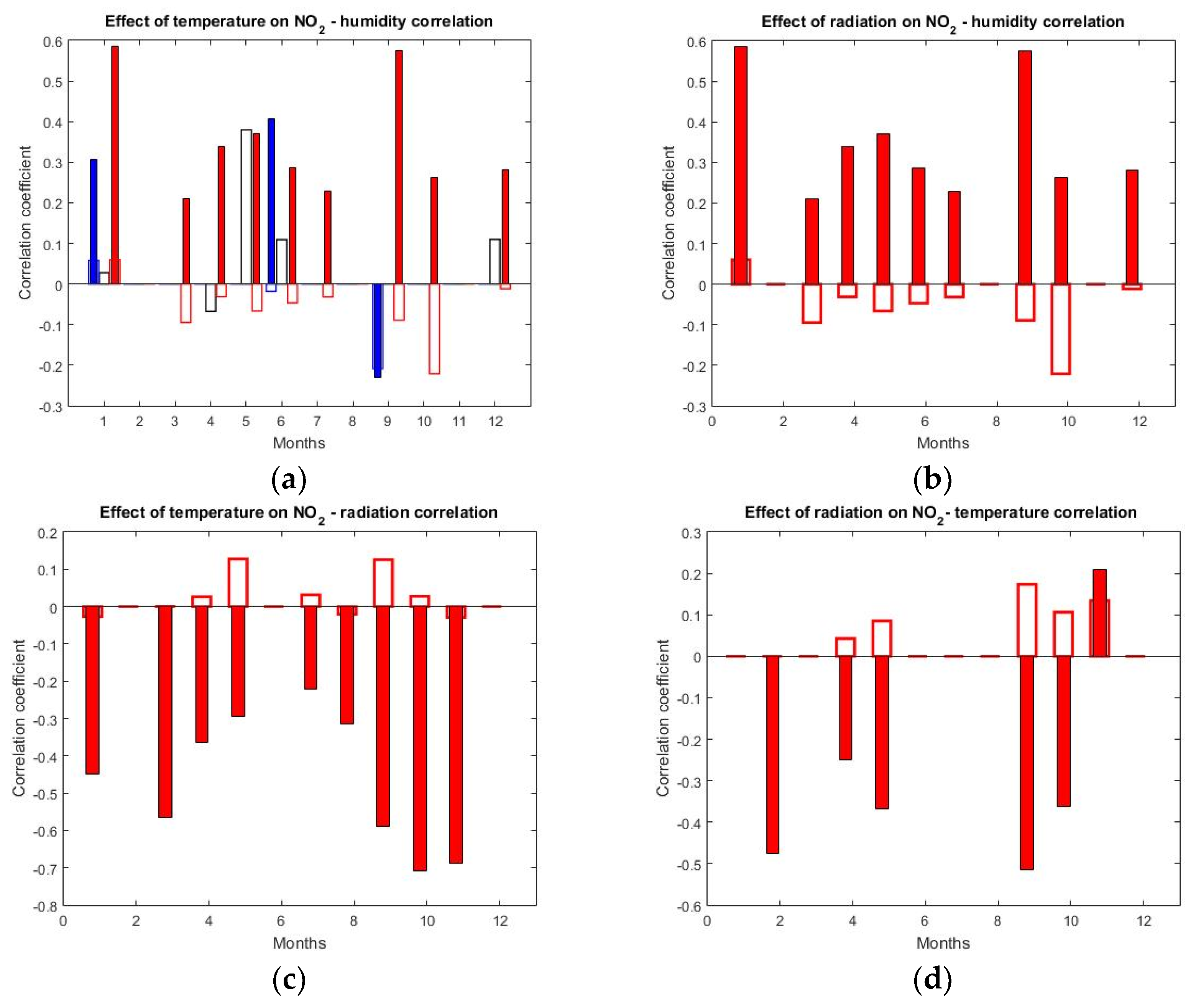
| C (Bivariate/Direct Correlation) | D = P − C | C × D | Correlation between X and Z | Role of the Intervening Variable (Y) |
|---|---|---|---|---|
| >0 | 0 | 0 | real (positive) correlation | none |
| >0 | <0 | <0 | partially spurious | partially responsible for the correlation |
| >0 | >0 | >0 | partially suppressed | partially masks the real correlation |
| 0 | any | 0 | fully suppressed | fully masks the real correlation |
| <0 | 0 | 0 | real (negative) correlation | none |
| <0 | <0 | >0 | partially suppressed | partially masks the real correlation |
| <0 | >0 | <0 | partially spurious | partially responsible for the correlation |
| any | =C | >0 | fully spurious | fully responsible for the correlation |
| Location | Temperature | Humidity | Wind Speed | Seasons | Reference |
|---|---|---|---|---|---|
| Egypt, Cairo | Insignificant | Negative | Negative | - | [13] |
| India, Surat | Insignificant | - | Negative | Summer Autumn | [14] |
| India, Jabalpur | Negative | Negative | - | - | [17] |
| Saudi Arabia, Makkah | Insignificant | Negative | Negative | - | [18] |
| Saudi Arabia, Dhahran | Negative | Positive | Negative | Summer | [20] |
| China, Beijing | Negative | Positive | Negative | - | [19] |
| China, Shanghai | Negative | Negative | Negative | - | [19] |
| China, Guangzhou | Positive | Negative | Negative | - | [19] |
| Malaysia Kuala Lumpur | Positive | Insignificant | Negative | - | [15] |
| Iran, Isfahan | Negative | Negative | Negative | - | [16] |
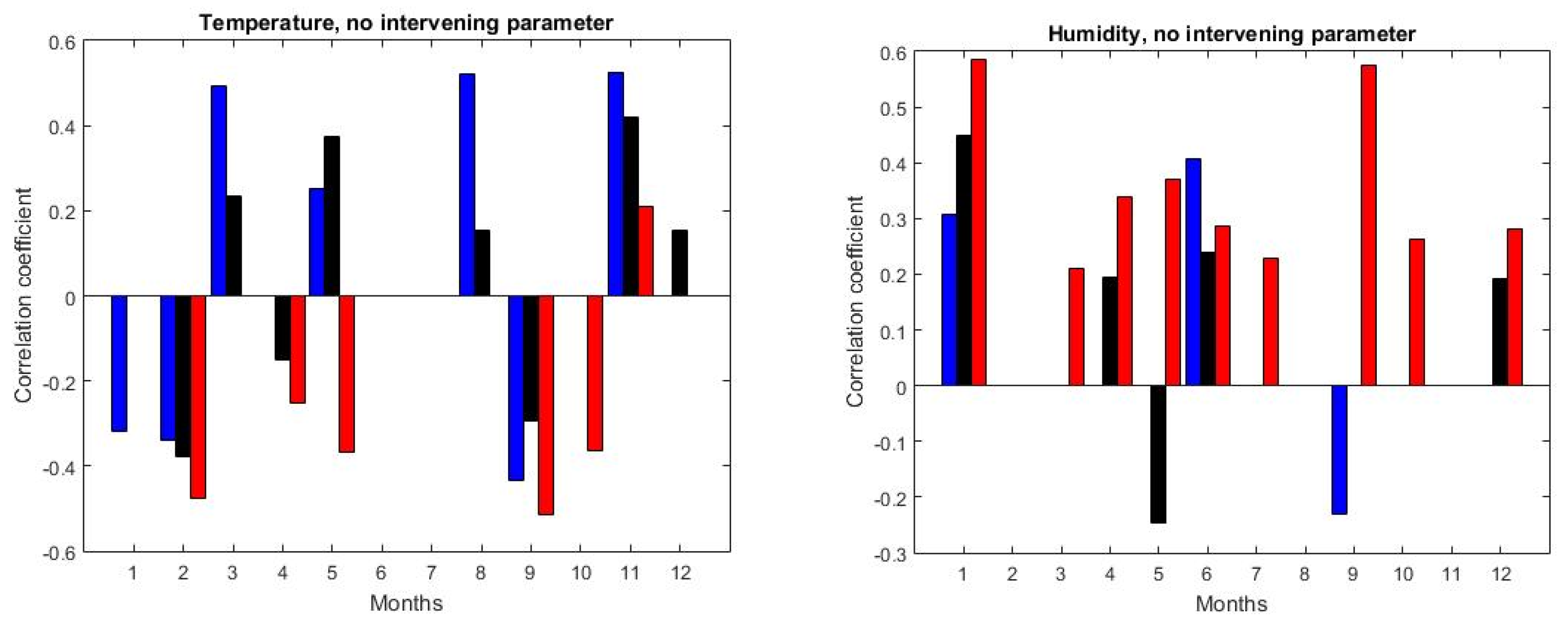
| Variable 1 (X) | Variable 2 (Z) | Intervening Variable (Y) | Plot in Figure 6 |
|---|---|---|---|
| NO2 | relative humidity | temperature | a |
| NO2 | relative humidity | radiation | b |
| NO2 | radiation | temperature | c |
| NO2 | temperature | radiation | d |
© 2020 by the authors. Licensee MDPI, Basel, Switzerland. This article is an open access article distributed under the terms and conditions of the Creative Commons Attribution (CC BY) license (http://creativecommons.org/licenses/by/4.0/).
Share and Cite
Voiculescu, M.; Constantin, D.-E.; Condurache-Bota, S.; Călmuc, V.; Roșu, A.; Dragomir Bălănică, C.M. Role of Meteorological Parameters in the Diurnal and Seasonal Variation of NO2 in a Romanian Urban Environment. Int. J. Environ. Res. Public Health 2020, 17, 6228. https://doi.org/10.3390/ijerph17176228
Voiculescu M, Constantin D-E, Condurache-Bota S, Călmuc V, Roșu A, Dragomir Bălănică CM. Role of Meteorological Parameters in the Diurnal and Seasonal Variation of NO2 in a Romanian Urban Environment. International Journal of Environmental Research and Public Health. 2020; 17(17):6228. https://doi.org/10.3390/ijerph17176228
Chicago/Turabian StyleVoiculescu, Mirela, Daniel-Eduard Constantin, Simona Condurache-Bota, Valentina Călmuc, Adrian Roșu, and Carmelia Mariana Dragomir Bălănică. 2020. "Role of Meteorological Parameters in the Diurnal and Seasonal Variation of NO2 in a Romanian Urban Environment" International Journal of Environmental Research and Public Health 17, no. 17: 6228. https://doi.org/10.3390/ijerph17176228