Differential Laser Doppler based Non-Contact Sensor for Dimensional Inspection with Error Propagation Evaluation

The University of Manchester, School of Mechanical, Aerospace and Civil Engineering. PO Box 88, Manchester, UK
*
Author to whom correspondence should be addressed.
Sensors 2006, 6(6), 546-556; https://doi.org/10.3390/s6060546
Submission received: 25 April 2006
/
Accepted: 13 June 2006
/
Published: 15 June 2006
(This article belongs to the Special Issue Intelligent Sensors)
Abstract
:To achieve dynamic error compensation in CNC machine tools, a non-contact laser probe capable of dimensional measurement of a workpiece while it is being machined has been developed and presented in this paper. The measurements are automatically fed back to the machine controller for intelligent error compensations. Based on a well resolved laser Doppler technique and real time data acquisition, the probe delivers a very promising dimensional accuracy at few microns over a range of 100 mm. The developed optical measuring apparatus employs a differential laser Doppler arrangement allowing acquisition of information from the workpiece surface. In addition, the measurements are traceable to standards of frequency allowing higher precision.
1. Introduction
Zero defect parts could only be obtained via full automatic error compensation while they are being machined on the next generation of intelligent machining processes to ensure high quality products at low price and short time. Off-line axis error compensation is successfully achieved with NC machines including thermal growths while on-line compensation still has some difficulties mainly with probes hardware and controllers [1-2]. Quality control of the manufactured parts is traditionally performed using manual inspection methods and statistical sampling procedures. It has the disadvantages of releasing some defective parts and using an inspection area. To overcome these problems, in-process inspection with error correction in NC machines is proposed as another alternative. In-process measurement techniques have been proposed over the last two decades to control the quality of a workpiece with some difficulties to be addressed. The trend principle in this type of inspection is to use a measuring probe with a measurement control system and to adjust machining parameters to reach the nominal dimension with the required accuracy. A Full review of the developed in-process methods since 1961 is discussed in Shiraishi [3], Yandayan and Burdekin [4], and, Vacharanukul and Mekid [5]. Optical measurement techniques have the advantage to be fast and contact less.
A variety of optical sensors are applied to measurement in metrology. The most common techniques include triangulation [6], shearing interference [7], coherence radar [8] and laser Doppler techniques [9]. Laser Doppler Velocimetry has proven to be very accurate and repeatable over years for fluid applications such as anemometry [10]. Also Laser Doppler system finds applications in length measurement of sheet materials (e.g. paper, textiles and foils) [11]. Recently, an indirect measurement method for the determination of the surface velocity in vibrating structures based on laser Doppler vibrometry was investigated [12].
In mass production, the diameter is one of the significant parameters to be inspected. Many measurement techniques have been developed to measure the diameter of a workpiece [5]. In this paper, an in-process laser Doppler technique is presented to measure a diameter of the moving workpiece. The fundamental method of differential Doppler technique is employed for solid material with an emitting laser kept clean from back lights using polarizer and retarder as well as an optical amplification of the scattered light. The Doppler signal is acquired in real-time and processed for noise reduction and FFT autocorrelation to accurately determine the Doppler frequency and hence the workpiece diameter. It is expected to enhance the accuracy of measurement up to very few micrometers over a range of 100 mm with a very good traceability of measurements as it uses Laser light as core component.
2. Theory
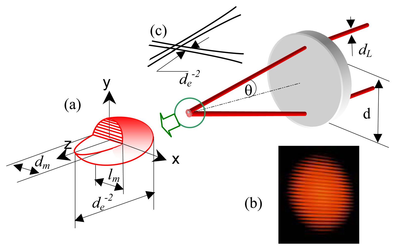
The principle of differential laser Doppler requires two beams to generate a measuring volume. The shape of the measuring volume is an ellipsoid as illustrated in Figure 1(a). The size of the measuring volume can be calculated by;
where de−2 is the waist diameter of the focused laser beams after the focusing lens (Figure 1(c)), dm and lm are respectively the transversal size and the longitudinal size of the measuring volume. de−2 can be approximately expressed as
where dL is the diameter of the laser beam and F is the focal length of the focusing lens [6]. The Doppler signal occurs when particles or a moving surface pass through the ellipsoidal measurement volume.
The light waves of two beams interfere with one another in the crossing region, creating an interference pattern which consists of parallel fringe planes (Figure 2(a)). The fringe spacing, df, is given by Eq.4, where θ is the angle between a beam and the optical axis and λ is the laser wavelength.
As the dimension of the measuring volume and the fringe spacing are defined, the number of fringes in the measuring volume Nf can be given by Eq.5.
The number of fringes can also be expressed in terms of optic and wavelength parameters in Eq.6.
Slightly different expressions were proposed in [13-14] to estimate the size of the measuring volume and the number of fringes depending on the crossing location of the beams for which the beam energy is calculated. The fringe counting has been checked with the current test-bench (Figure 1(b)) and it was found that expression shown in Eq.6 is more accurate compared to those proposed in [13-14]. Moreover, the occurrence of fringes depends on the properties of light source. One main property is called ‘the coherence length’. If the optical path difference between two beams is less than the coherence length, fringes will occur. Thus, the coherence length is one constraint for the optical arrangement based on the differential Doppler technique. The coherence length, ΔLc, is determined by Eq.7.
The scattered light is collected by a photo detector which generates an electrical signal. The measurement of the object velocity is converted into frequency measurement of the electrical signal with a scale factor. As the frequency measurement can be easily performed in a wide span of frequencies up to 100 MHz, the fluid velocity can therefore be measured from low to high velocities. A particle crossing through the interference region in Figure 2(a) will develop a clean oscillation with a Gaussian envelope as the laser operates in the TEM00 mode. This is the Transverse Electromagnetic Modes (TEM) of the laser beam, which is the wave pattern on the output aperture plane. This particular mode (TEM00) has circular symmetry and a Gaussian profile as shown in Figure 2(b). The signal becomes weaker as the particles cross away from the center of the interference region.
3. laser probe description
A non-contact, in-process dimensional probe has been developed to measure workpiece diameter based on the differential laser Doppler technique. The basic principle of the arrangement is to generate fringes on the workpiece surface where the circumferential velocity is normal to the fringe pattern and to detect the Doppler signal obtained from the scattered lights. The probe is shown in Figure 3. A laser beam is split into two beams whose parallelism is secured by a right angle prism. The beams go through the focusing lens and cross at the focal length. The scattered light from the workpiece surface is collected by a lens and a photodetector. However, some reflected lights and the scattered lights from the workpiece surface can return back to the laser head causing a chaos in the emitting laser. Hence a polarizer and a retarder are placed in front of the laser head to block these lights before they reach the laser head. If the laser light passes through a polarizer and a retarder, respectively, the output light will be a circular or elliptical. Lights reflected and scattered from the workpiece surface have possibly other planes of polarization compared to the incident beam. As a result, the reflected lights and the scattered lights should probably be stopped or at least decreased.
The laser light is scattered from the moving surface passing through the fringes. It oscillates with a specific frequency that is related to the velocity of the workpiece. The workpiece diameter can be calculated using the relationship between the circumferential velocity, V, and the rotation speed, N, which equation is shown as follow:
where D is the diameter of the workpiece and N is the number of revolutions per minute. According to Eq.7 and Eq.9, the Doppler frequency relates to the circumferential velocity of the workpiece depending on the angular velocity and the diameter of the workpiece. By revising the Doppler frequency equation, the diameter of a workpiece, D, is given by Eq.10.
When a particle in fluid or gas passes through the fringe volume, a burst of Doppler signal occurs. Scattering from a diffusing solid surface can be considered equivalent to a multitude of particles distributed randomly in the measuring volume for flow measurements. Figure 4 (b) shows a typical signal from a solid workpiece surface with the current probe. The signal includes Doppler signal with noises. These low-frequency noises can be eliminated using a high-pass filter. The acquired signal was processed by fast Fourier transformations (FFT) technique. The spectrum is fitted with a Gaussian distribution to locate neatly the centre frequency (Figure 4(a)). The standard deviation of the centre frequency (σfc) is given by Eq.11.
4. Parameters affecting the accuracy of diameter measurement and error propagation
As this is not a direct measurement, the accuracy of the diameter measurement depends on the performance of its components. A unified method for the evaluation and expression of measurement uncertainties is published within the Guide to the expression of Uncertainty in Measurement (GUM) [15] which is accepted worldwide. The combined standard uncertainty, uc, as the standard uncertainty of the measurement of Y, by combining the individual standard uncertainties and co-variance, depending on the case and using the law of propagation of uncertainty:
where ∂f/∂xi are the partial derivatives ∂f/∂Xi evaluated at Xi = xi and u(xi , xj)are the estimated co-variance associated with xi and xj.
Eq.13 is based on a first-order Taylor series approximation of
Where Y is the measurand determined from N input quantities X1, X2,,…, XN through a functional relationship f. An estimate of the measurand Y, represented by y, is obtained from Eq.13 using input estimates x1, x2,…, xN for the values of the input quantities. The output estimate which is the results of measurement is then given by
The performance of each component for the in-process laser probe considered in this paper as well as the propagation of uncertainty are discussed hereafter. Other source of errors may be induced by beams misalignment and adjustment.
4.1 Accuracy of He-Ne Laser
A He-Ne laser is recognised to have a narrow variation in wavelength, which generally falls within a range of 10-12 m. The wavelength stability depends on the linewidth of the laser. The change in the wavelength due to the linewidth, Δλ, can be calculated by:
Where λ is the wavelength of the laser, c is the light speed in vacuum and Δν is the spectral linewidth of the He-Ne laser (1.5GHz). By substituting λ = 632 nm into Eq.16, Δλ is approximately 0.002 nm. This variation causes an error in the diameter measurement based on the differential Doppler technique. The error owing to the wavelength variation at 0.002 nm for a 100 mm diameter workpiece at 1000 rpm and at θ = .7.125° is shown in table 1. Therefore the error in diameter will be approximately 0.3 μm. Thus, the effect of the laser wavelength on the required accuracy of diameter measurement of micrometer is considered acceptable.
4.2 Accuracy of the Doppler frequency
As Gaussian fit is applied to determine the Doppler frequency, the relative accuracy of the Doppler frequency measurement, σf/fd is determined by equations 11 and 12 and is less than 0.01%.
4.3 Accuracy of the beam crossing angle
The angle between a beam and the optical axis is given by Eq.17.
4.4 Accuracy of the number of revolutions per minute
In general the number of revolutions per minute is measured using timers and counters within the motion controller card but usually the value is acquired from the NC machine controller. The accuracy of rotative speed is better than 0.01%.
4.5 Error Propagation
The error propagation has been calculated in this indirect measurement comprising the previous described four parameters with the associated estimated errors. The diameter which is calculated from Eq.10 can be expressed into a more general form as shown in Eq.18.
The overall expression of the error propagation of the first order has been derived from Eq.13 as shown in Eq.19.
5. Experimental setup and calibration
During the construction of the probe, a test bench has been built to host a laser source emitting a stable laser beam which is split into two beams. The two beams are aligned at long distance. The beams go then through an acromat lens and are focused on the workpiece surface. The workpiece is rotated with stable, controlled angular speed at the relative accuracy of <0.5%. The scattered light is focused onto the photodiode using a single biconvex lens. An electronic circuit has been developed to amplify the signal and to filter it in high pass mode as the Doppler frequency is workpiece diameter and rotation speed dependant. The signal processing is developed under LabView environment with real time data acquisition. The signal spectrum is calculated by FFT. A Gaussian fit to locate the centre of the spectrum which yields the Doppler frequency.
An auto focus system may be required to keep the measuring ellipsoid volume within the workpiece skin. If the workpiece has larger radial vibrations, measurement could be interrupted as shown in Figure 5. Usually any radial vibration should be within the ellipsoid length. The probe has been calibrated over the range of measurement against four different reference diameter parts (25, 50, 75 and 100mm.) inspected accurately with a CMM machine. As a result, the factor, which represents the relationship between the Doppler frequency and speed, can be evaluated from the calibration process.
6. Tests and results
Extensive tests have been carried out on various diameters up to 100 mm. A sample of measurements is presented in this paper. Two identical dimension workpieces with different surface roughness values were rotated in a CNC machine. The workpiece diameters were measured using the current probe. The results of the measurements are shown in table 2. The measurements were taken at 550 rpm and the Doppler frequency for the diameter of 30 mm was 183 kHz with an uncertainty of 22 Hz which is less than 0.012%. The maximum systematic error for the measurements is within 10 μm over a range of 100 mm.
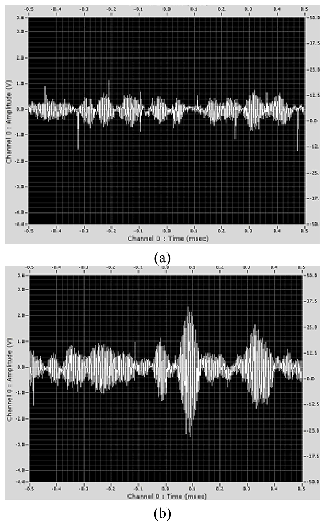
The aim of testing the probe with two workpieces having different surface roughness is to investigate whether the surface roughness affects to the probe. Figure 6 shows that the rougher workpiece generates more back-scattered light intensity than the smoother workpiece does. This may occur as the rougher workpiece provides more scattered points.
7. Conclusion
An in-process and non-contact dimensional measurement sensor has been presented in this paper. The performance of the differential laser Doppler technique applied to solid material has been demonstrated through various tests and diameter measurements. The overall accuracy depends on the accuracy performance of the probe components. The measurements have shown very good accuracies but it is believed that these could be improved according to the theory. The effects of thermal growth should be taken into account although the probe is usually to be used for predictive action near finishing passes to control the final accuracy.
The differential laser Doppler technique seems to be well suited for non-contact dimensional measurement. With the traceability of measurements, further developments are expected to quantify the errors of form that a workpiece may have such as roundness and eccentricity. The work is also extended to profile determination.
References
- Soons, J.A.; Theeuws, F.C.; Schellekens, P.H. Modelling the errors of multi-axis machines: a general methodology. Precision Engineering 1992, 14(1), 5–19. [Google Scholar]
- McKeown, P.A.; Weck, M.; Bonse, R. Reduction and compensation of thermal error in machine tools. Annals of the CIRP 1995, 44(2), 589–593. [Google Scholar]
- Shiraishi, M. Scope of in-process measurement, monitoring, control techniques in machining processes. Precision Engineering 1989, 11(1), 27–37. [Google Scholar]
- Yandayan, T.; Burdekin, M. In-process dimensional measurement and control of workpiece accuracy. Int. J. Machine Tools and Manufacture 1997, 37, 1423–1439. [Google Scholar]
- Vacharanukul, K.; Mekid, S. In-process dimensional inspection sensors. Measurements 2005, 38, 204–218. [Google Scholar]
- Dorsch, R.G.; Hausler, G.; Herrmann, J.M. Laser triangulation: fundamentals uncertainty in distance measurement. Applied Optics 1994, 33(14). [Google Scholar]
- Hausler, G.; Hermann, J.M. Range sensing by shearing interferometry: influence of speckle. Applied Optics 1988, 27(7), 4631–4637. [Google Scholar]
- Dresel, T.; Hausler, G.; Venske, H. Three-dimensional sensing of rough surfaces by coherence radar. Applied Optics 1992, 31(25), 919–925. [Google Scholar]
- Sriram, P.; Hanagund, S.; Craig, J.; Komerath, N.M. Scanning laser Doppler technique for velocity profile sensing on a moving surface. Applied Optics 1990, 29(17), 2409–2417. [Google Scholar]
- Absil, L. H. J. Analysis of the laser Doppler measurement technique for application in turbulent flows; Deft University of Technology: Netherlands, 1995. [Google Scholar]
- Stork, W.; Wagner, A.; Kunze, C. Laser Doppler sensor for speed and length measurements at moving surfaces. Proceedings of SPIE 2001, 4398, 106–115. [Google Scholar]
- Martarelli, M.; Revel, G.M. Laser Doppler vibrometry and near-field acoustic holography: Different approaches for surface velocity distribution measurements. Mechanical Systems and Signal Processing 2006, 20, 1312–1321. [Google Scholar]
- Durrani, T. S.; Greated, C. A. Laser systems in flow measurement; Plenum Press: New York and London, 1977. [Google Scholar]
- Donati, S. Electro-optical instrumentation: sensing and measuring with lasers; Prentice Hall PTR, 2004. [Google Scholar]
- Guide to the expression of uncertainty in measurement.; International Organisation for Standardization (ISO): Geneva, 1995.
Figure 1.
Ellipsoid of fringes and measuring volume parameters.

Figure 2.
(a) The interference pattern caused by crossing between two beams. (b) TEM00 mode.
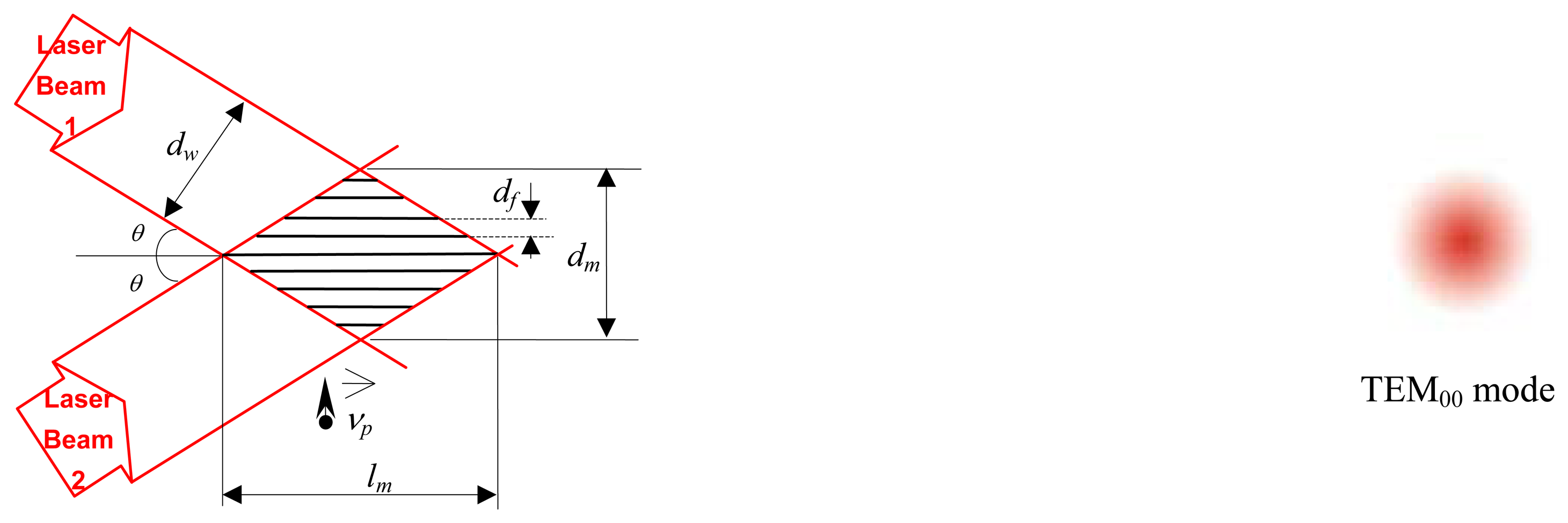
Figure 3.
Differential Doppler technique probe and its location on a Takisawa lathe machine.
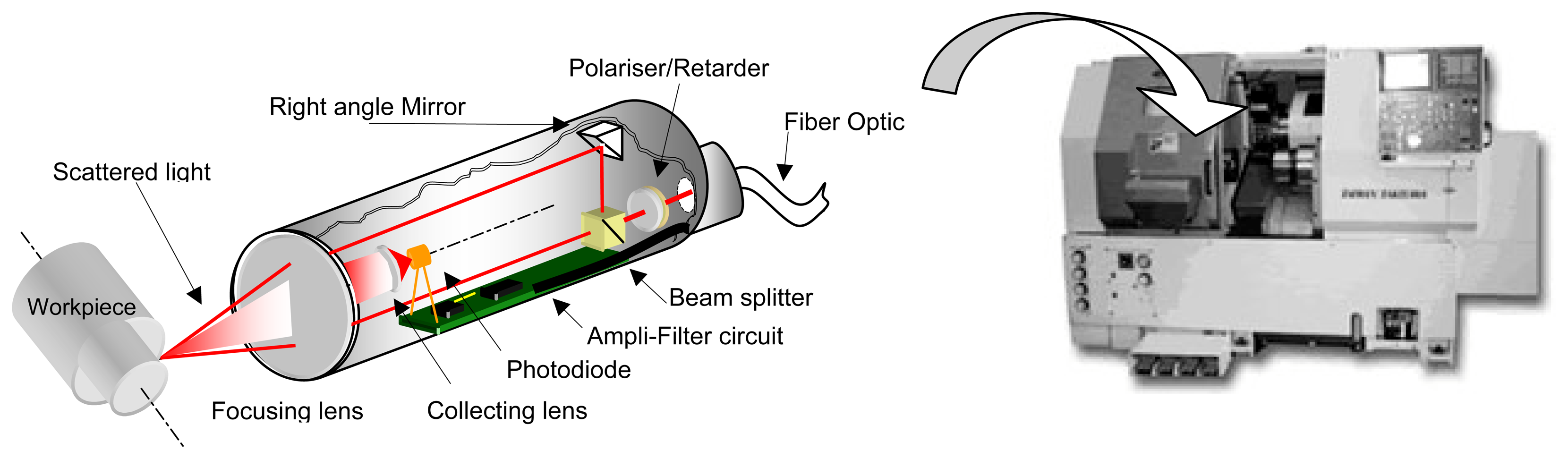
Figure 4.
(a) Data Spectrum with Gaussian fit, (b) Bursts of Doppler signal from solid surface.
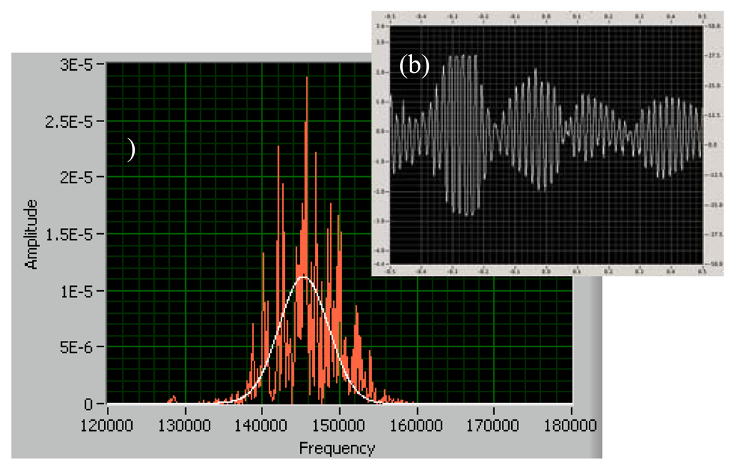
Figure 5.
Radial vibration limit of the workpiece to achieve measurement.
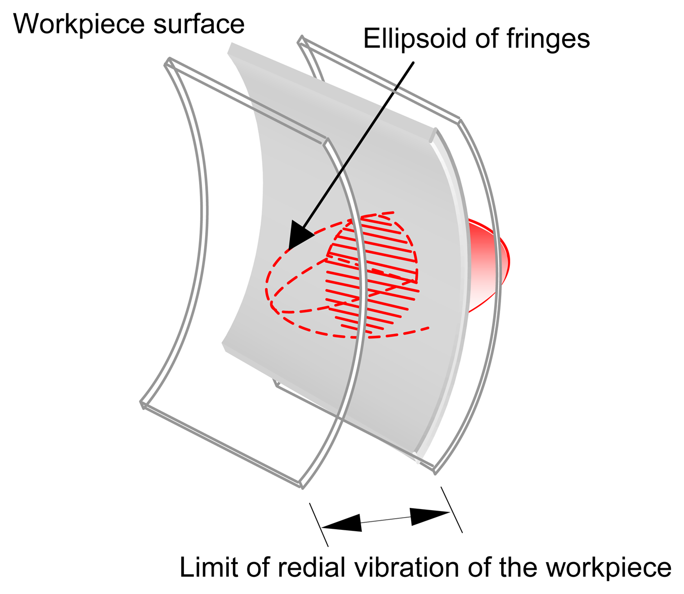
Figure 6.
The Doppler signal from two different surface roughness workpieces; (a) from the smoother workpiece and (b) from the rougher workpiece.
Figure 6.
The Doppler signal from two different surface roughness workpieces; (a) from the smoother workpiece and (b) from the rougher workpiece.

| λ [nm] | fd [Hz] |
|---|---|
| 632.000 | 2055203.644 |
| 632.002 | 2055197.141 |
| Workpiece 1 (Ra=0.080μm) | Workpiece 2 (Ra=0.145μm) | ||
|---|---|---|---|
| D [mm] | δD [μm] | D [mm] | δD [μm] |
| 30.006 | 3.4 | 30.274 | 5.5 |
| 50.037 | 3.7 | 50.294 | 5.8 |
| 70.099 | 5.7 | 70.325 | 7.1 |
| 90.154 | 8.8 | 90.256 | 9.8 |
© 2006 by MDPI ( http://www.mdpi.org). Reproduction is permitted for noncommercial purposes.
Share and Cite
MDPI and ACS Style
Mekid, S.; Vacharanukul, K. Differential Laser Doppler based Non-Contact Sensor for Dimensional Inspection with Error Propagation Evaluation. Sensors 2006, 6, 546-556. https://doi.org/10.3390/s6060546
AMA Style
Mekid S, Vacharanukul K. Differential Laser Doppler based Non-Contact Sensor for Dimensional Inspection with Error Propagation Evaluation. Sensors. 2006; 6(6):546-556. https://doi.org/10.3390/s6060546
Chicago/Turabian StyleMekid, Samir, and Ketsaya Vacharanukul. 2006. "Differential Laser Doppler based Non-Contact Sensor for Dimensional Inspection with Error Propagation Evaluation" Sensors 6, no. 6: 546-556. https://doi.org/10.3390/s6060546