A Pattern-Recognition-Based Ensemble Data Imputation Framework for Sensors from Building Energy Systems


National Renewable Energy Laboratory, Buildings and Thermal Sciences Center, Golden, CO 80401, USA
Sensors 2020, 20(20), 5947; https://doi.org/10.3390/s20205947
Submission received: 12 September 2020
/
Revised: 12 October 2020
/
Accepted: 19 October 2020
/
Published: 21 October 2020
(This article belongs to the Section Intelligent Sensors)
Abstract
:Building operation data are important for monitoring, analysis, modeling, and control of building energy systems. However, missing data is one of the major data quality issues, making data imputation techniques become increasingly important. There are two key research gaps for missing sensor data imputation in buildings: the lack of customized and automated imputation methodology, and the difficulty of the validation of data imputation methods. In this paper, a framework is developed to address these two gaps. First, a validation data generation module is developed based on pattern recognition to create a validation dataset to quantify the performance of data imputation methods. Second, a pool of data imputation methods is tested under the validation dataset to find an optimal single imputation method for each sensor, which is termed as an ensemble method. The method can reflect the specific mechanism and randomness of missing data from each sensor. The effectiveness of the framework is demonstrated by 18 sensors from a real campus building. The overall accuracy of data imputation for those sensors improves by 18.2% on average compared with the best single data imputation method.
1. Introduction
It is reported by U.S. Energy Information Administration that buildings consumed 32% of primary energy in 2019 in the United States and global energy consumption in buildings will grow by 1.3% per year on average from 2018 to 2050 [1]. Building operation data are playing an important role in building design, retrofit, commissioning, maintenance, operations, monitoring, analysis, modeling, and control. With the wide adoption of building automation system (BAS), smart sensors, and Internet of Things in buildings, massive measurements from sensors and meters are continuously collected, providing a +great amount of data on equipment and building operations and great opportunities for data-driven tools to improve building energy efficiency based on collected data [2].
Data quality is essential for data-driven tools and missing data is one of the most common and important issues for data quality. During building operations, it is common for sensors to fail to record data for several reasons, including malfunctioning equipment or sensors, power outage at the sensor’s node, random occurrences of local interferences, and a higher bit error rate of the wireless radio transmissions as compared with wired communications [3]. Cabrera and Zareipour [4] summarized that missing data can be grouped depending on the reason they are missing: (a) missing not at random, or systematic missing: when the probability of an observation being missing depends on the information that is not observed; (b) missing at random: when the probability of an observation being missing depends on other observed values; and (c) missing completely at random: when the probability of an observation being missing is completely at random and not related to any other value.
In statistics, imputation is the process of replacing missing data with substituted values [5]. The theories of imputation are well studied. Early in 2001, Pigott [6] wrote a review of methods for missing data imputation and he summarized that ad hoc methods, such as complete case analysis, available case analysis (pairwise deletion), or single-value imputation, are widely studied. Ad hoc methods can be easily implemented, but they require assumptions about the data that rarely hold in practice. However, model-based methods, such as maximum likelihood using the expectation-maximization algorithm and multiple imputation, hold more promise for dealing with difficulties caused by missing data. While model-based methods require specialized computer programs and assumptions about the nature of the missing data, these methods are appropriate for a wider range of situations than the more commonly used ad hoc methods. Harel and Zhou [7] reviewed some key theoretical ideas, forming the basis of multiple imputation and its implementation, provided a limited software availability list detailing the main purpose of each package, and illustrated by example the practical implementations of multiple imputation, dealing with categorical missing data. Ibrahim et al. [8] reviewed four common approaches for inference in generalized linear models with missing covariate data: maximum likelihood, multiple imputation, fully Bayesian, and weighted estimating equations. They studied how these four methodologies are related, the properties of each approach, the advantages and disadvantages of each methodology, and computational implementation. They examined data that are missing at random and nonignorable missing. They used a real dataset and a detailed simulation study to compare the four methods.
Many existing studies are found to apply data imputation in missing data in buildings. Deleting the missing data is the most direct way to deal with them and, on some occasions, it can be counted as a data imputation method. In the research from Ekwevugbe et al. [9], all corrupted and missing data instances due to instrumentation limitations were excluded from further analysis. Xiao and Fan [10] addressed that missing values can be filled in using the global constant, moving average, or inference-based models. In their paper, missing values were handled using a simple moving average method with a window size of five samples. Rahman et al. [11] proposed an imputation scheme using a recurrent neural network model to provide missing values in time series energy consumption data. The missing-value imputation scheme has been shown to obtain higher accuracies than those obtained using a multilayer perceptron model. Peppanen et al. [12] presented a novel and computationally efficient data processing method, called the optimally weighted average data imputation method, for imputing bad and missing load power measurements to create full power consumption data sets. The imputed data periods have a continuous profile with respect to the adjacent available measurements, which is a highly desirable feature for time-series power flow analyses. Ma et al. [13] proposed a methodology called the hybrid Long Short-Term Memory model with Bi-directional Imputation and Transfer Learning (LSTM-BIT). It integrates the powerful modeling ability of deep learning networks and flexible transferability of transfer learning. A case study on the electric consumption data of a campus lab building was utilized to test the method.
To summarize the above research, researchers introduced, developed, and applied a specific imputation method applied for specific sensor types and missing data scenarios. However, normally in one building system, there are various types of sensors, including a thermometer, humidity sensor, flow meter, energy meter, differential pressure sensors, etc. There are also multiple missing data mechanisms (malfunction, power outage, local interferences, wireless radio transmissions error) and multiple randomness for missing data (missing not at random, missing at random, missing completely at random) for various sensors. The single imputation method may not be able to capture various missing data scenarios from various sensors. Few researchers study the compatibility of a single technique on various sensors with missing data. A few papers are found to work on the selection and use of multiple data imputation methods and they are introduced in the following paragraph.
Inman et al. [14] explored the use of missing data imputation and clustering on building electricity consumption data. The objective was to compare two data imputation methods: Amelia multiple imputation and cubic spline imputation. The results of this study suggest that using multiple imputation to fill in missing data prior to performing clustering analysis results in more informative clusters. Schachinger et al. [15] focused on improving and correcting the monitored data set. They tried to identify the reasons for data losses and then look for recovery options. If lengths of periods of missing data are not exceeding the predefined thresholds, these periods are interpolated. Interpolation thresholds are set depending on the frequency of sensor monitoring and dynamic behavior. Continuous data are interpolated using linear and polynomial interpolation. Habib et al. [16] filled the missing values with regression and linear interpolation for short and long periods. They also addressed that (a) it is necessary to detect the missing gaps between the data acquired as it is also an important factor to indicate the reliability of the data, (b) these missing gaps are always undeniable and lowering the amount of meaningful calculations, (c) it is crucial to make the missing gaps fewer as data with fewer gaps is considered good quality data, and (d) there are different methods available for handling the missing values, e.g., regression, depending on the nature of the data and other parameters, such as computations, precision, robustness, and accuracy. Xia et al. [17] addressed that to get the data in workable order for calculation, analysis, and benchmarking, the missing or invalid (mainly negative) data should be replaced with data during time periods or days that were similar to the invalid points, taking weather condition into account as well. For example, a few missing data would be replaced by the previous or following few proper data, or their average. Several hours’ missing data would be replaced by data of the same time periods on the previous or following day, considering weekdays and weekends. The same goes for missing or invalid data of an even longer period. Garnier et al. [18] used data anterior and/or posterior to the sensor failure in order to rebuild the missing information. Two different approaches were presented: an interpolation technique used for the estimation of missing solar radiation data and an extrapolation technique based on artificial intelligence deals with indoor temperature estimation.
The papers in the last paragraph addressed the selection among only a few (two or three) imputation methods according to the length of missing data gaps, sensor types, and the nature of missing data. Too much domain knowledge is set to select among the sensors, making the method less automated. Ensemble method, which is a pool-based method that can better address the variation problem is rarely applied for building sensors. Additionally, few studies are found to apply the ensemble method to customize the imputation for different sensors with missing data.
One more key issue for data imputation techniques lies in the difficulty of validation. Since the information of missing data are missed already and the truth data is lost forever, it is hard to create some testing or validation scenarios to quantify the performance of data imputation methods.
In this paper, a framework is proposed to deal with the above two problems. First, a validation module is developed based on pattern recognition. This module identifies good data points that have similar characteristics with the missing data. The selected good data can mimic missing data but with truth value, which create testing scenarios to validate the effectiveness of the single data imputation method. Second, with the validation data decided, a pool of data imputation methods is tested under the validation dataset, to find an optimal imputation method for each sensor, which is basically an ensemble method. The selected imputation method is expected to be different from sensor to sensor, which can optimize the accuracy of imputation under different sensor types and different mechanism and randomness of data missing for each sensor.
2. Pattern-Recognition-Based Ensemble Data Imputation Framework
The data imputation framework addresses two problems summarized in Section 1: (1) the lack of validation data to test imputation methods, and (2) the lack of method to automatically customize the imputation method for various sensors with various mechanism and randomness of missing data. Correspondingly, there are two modules to solve the problem, respectively, which are: the validation data generation module (Module 1) and the ensemble imputation module (Module 2). The diagram of the framework and the two modules are shown in Figure 1.
2.1. Module 1. Validation Data Generation
As shown in Figure 1, the original timeseries data have good values (green square) and missing data (red square). Module 1 creates validation data (yellow square) using pattern recognition technique. Data with good values (e.g., x7 and x8 in Figure 1) and the generated validation data (x’7 and x’8) are the same in terms of values; their only difference is that the validation data are used to evaluate the imputation method. Pattern recognition is applied to identify some good data points that have similar characteristics with the missing data (red square) and marks them as validation data. The characteristics include time indicators (such as hour of day, day of week, weekday weekend indicator, and month of year) and weather variables (such as outdoor air temperature, humidity, and solar radiation). This means that the pattern recognition technique tries to search among good data and find the ones that have similar happening time and weather condition with the missing data, trying to mimic the missing data mechanism. Similarity metrics such as Euclidean distance are used to quantify how missing data and good data are similar with each other. To be more specific, the problem can be formulated and simplified using the equation representing that the method tries to search among all good data () to select several good data points (, a matrix with time and weather variable) with the highest similarity metrics (defined by ), meaning they are the most similar to the missing data set (). The selected good data points are supposed to be more likely to miss values. Those data sets that are similar to missing data but have a truth value can be further used as validation datasets to test the effectiveness of data imputation methods in the next steps. The pattern recognition techniques can be unsupervised clustering techniques (such as K-means clustering, categorical mixture models, hierarchical clustering, correlation clustering, and kernel principal component analysis), supervised classification techniques (such as neural network, support vector machine, decision tree and random forest), and any other statistical methods that can classify and cluster data.
2.2. Module 2. Ensemble Imputation Method
After deciding the validation dataset in Module 1, Module 2 applies the ensemble method to find the data imputation method with the best validation accuracy among a pool of imputation methods for each sensor using the validation dataset. First, it creates a pool of data imputation methods including statistical and model-based methods, for example simple (e.g., nearest available value), linear (e.g., linear interpolation), nonlinear (e.g., quadratic interpolation), piecewise (e.g., piecewise polynomial interpolation), and machine-learning-based interpolation (e.g., support vector machine). Since it is an ensemble method whose performance depends on the method with the best performance, the more diversified and more imputation methods are in the pool, the better performance this ensemble method can achieve. Then, it tests each imputation method using the validation dataset generated in Module 1 and selects the method with the highest validation accuracy from the data imputation method pool for each sensor. The validation accuracy is quantified by some accuracy and error metrics (such as coefficient of variation of root mean squared error and r-squared) between the imputed value and the truth value of the validation data. Finally, all missing data are imputed by the selected data imputation method (blue square shown in Figure 1).
The developed framework can work if there is archiving system to store and manage history data. There is no additional cost on installation. The only cost to apply this framework is the hardware cost for computation. The output of the framework is post-processed and repaired missing data. It can be used for both online and offline missing data imputation, but, in this paper, only an offline process is considered. To demonstrate the application and the effectiveness of the framework, it is applied to the sensors from a real campus building in the next section.
3. Real-Building Case Study
3.1. Sensors from a Real Campus Building
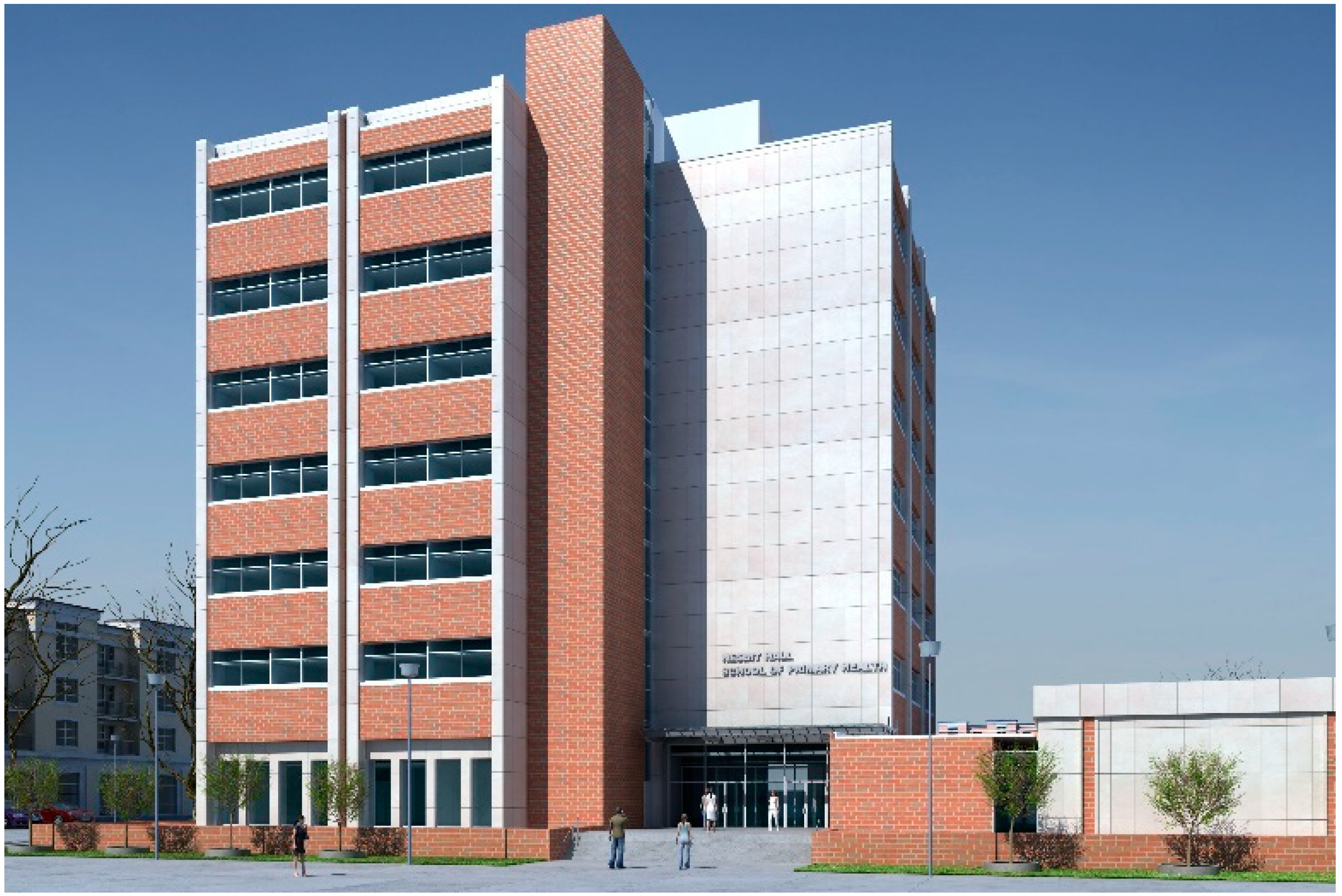
The sensors from Nesbitt Hall are used to demonstrate the developed framework. Nesbitt Hall (Figure 2) is a campus building located at Drexel University in Philadelphia. It is a seven-story, 7246 m2 commercial building that includes classroom, office, and laboratory space. It has one chiller and two steam-to-hot-water heat exchange systems. It has three air handling units (AHUs) located in the basement and on the roof. The chiller system is in the basement with the corresponding cooling tower on the top of the building. More details about heating, ventilation, and air conditioning (HVAC) systems and equipment of Nesbitt Hall can be found in Appendix A.
Among the 539 sensors from Nesbit Hall, 18 sensors with missing data listed in Table 1 are selected to test the framework. There are five considerations of choosing these sensors for the case study: (1) the sensors have adequate missing data; (2) the sensors are typical sensors in BAS; (3) the sensors cover various sensor types, including an energy meter, flow meter, thermometer, humidity sensor, ampere meter, valve position, and differential pressure sensors; (4) the sensors cover various equipment, including a chiller, AHU, and a variable-air-volume (VAV) box, and (5) the sensors have various patterns and characteristics of missing data, including missing data size and randomness. The data are downloaded via the Nesbitt Hall BAS web interface from 1st January to 16th August in 2017, which covers summer, winter, and shoulder seasons. Data are collected every 5 min (i.e., with a 5-min sample interval).
3.2. Missing Data Description of Selected Sensors
In Section 3.2, missing data characteristics, including missing data size and missing data randomness, are introduced. In terms of missing data size, Table 2 shows the total number of missing data and maximum holes (or gaps, meaning length of consecutive missing data) for each sensor. Table 2 indicates a varieties of missing data size for the selected sensors.
Most sensor data listed in Table 1 are systematically missed. The best example is the chiller energy meter. Figure 3 shows the Kernel Density Estimation plot reflecting density distribution of missing data happening time (hour of day). It shows that data are more frequently missed during the chiller’s start-up time (around 7–8 am) of the HVAC system, where energy suddenly increases. This indicates that the missing mechanism of chiller energy meter data is somehow systematic and not random. In this study, the systematic missing of each sensor are quantified by the randomness of time indicators for the time when data are missing, including hour of day, day of week, month of year, and weekday indicator (0 for weekday and 1 for weekend). For example, the randomness for the energy meter in terms of hour of day is low because data are missed following a pattern of fault happening time, or data are systematically missing in terms of hour of day in energy meters. We use a statistical test to quantify the randomness of missing data in this study. The null hypothesis is that the data are generated in a random manner, and the equation of randomness is shown in Equation (1), which can be found in the book [19]. In Equation (2), R is the number of runs. The concept of run is defined as a series of consecutive positive (or negative) values of the difference between one data point and the median of all data. n1 is the number of data that is greater than the median of all data, and n2 is the number of data that is less than the median.
The calculated Z-score indicates the randomness of a series of data: under a 10% significance level, the Z-score over 1.65 indicates non-randomness of data. The results of missing data randomness quantification by Z-score by sensor and time indicator are shown in Table 3. By comparing the calculated Z-score, missing data in sensors such as “chws_control/chw_flow” and “peco_meter/elec_usage_chiller” are more systematically missed, while sensors such as “ahu1/htg_stm_vlv_1_3” and “ahu1/stat_press” are less systematically missed. To compare the average of Z-scores among the time indicators, the missing mechanism seems less random and more correlated with hour of day. In other words, the missing data in most sensor are missed under some hourly pattern. It is worth mentioning that this paper will not study the truth of the mechanism of missing data in each sensor but only describe general randomness using Z-score. Moreover, the randomness test is not part of the framework, but it will help readers to better understand the characteristics of missing data for each sensor in the case study.
3.3. Create Validation Dataset
A random-forest-based pattern recognition technique is applied to the case study to create the same number of validation data (or “fake” missing data) from good data, by mimicking the real missing data characteristics. Pattern recognition here means we want to recognize the pattern of real missing data to find some good data with similar characteristics with real missing data, so that we can use those good data as validation dataset to test various data imputation methods.
We apply a supervised random-forest-based pattern recognition technique to realize the generation of validation dataset, or “fake” some missing data but with truth value. For each sensor, we label the missing data with 1 and good data with 0, which is the output of a random forest regressor. The inputs for the regressor are weather and time indicators, including outdoor air temperature, outdoor humidity, outdoor air enthalpy, hour of the day, day of the week, weekday indicator (0 for weekday and 1 for weekend), and month of the year. All the information from inputs are from timestamp of sensors and the corresponding weather that is recorded at the timestamp. We train the regressor based on the inputs and output. The model can predict under what time and weather the sensor will possibly miss a value. With that trained model, test the training inputs again and check the value of the output. The larger the testing output (or closer to 1), the more likely the data has the characteristics of missing data in terms of time and weather. Besides the n real missing data from one sensor, selected the other n good data with the highest testing output, which will show similar characteristics with the real missing data. Figure 4 shows an example of how a validation data point is generated based on its similar characteristics with one of the missing data in the chiller energy meter. The random forest algorithm is realized by a Python machine-learning library called scikit-learn. The parameters of random forest algorithm are all set to default.
3.4. Pool of Data Imputation Methods
As introduced in Section 2, the developed framework applies the ensemble method for missing data imputation, where multiple imputation methods are used as candidate methods to test the performance on the validation dataset. The method with the best validation accuracy will be the final imputation method for a specific sensor Table 4. lists a pool of the candidate data imputation methods for the real-building case study. The ensemble method is independently conducted for each sensor, meaning that one single imputation method will be selected for each sensor. As can be seen from Table 4, there are five categories of the imputation methods in the pool for the case study: (1) simple interpolation using the next, last, or nearest valid observation to fill the missing data gap (bill, ffill, and nearest); (2) linear interpolation (linear); (3) nonlinear interpolation (quadratic and cubic); (4) piecewise splines (piecewise_polynomial, from_derivatives, pchip, akima); and (5) machine-learning-based interpolation techniques (artificial neural network, or ANN). These data imputation methods are realized by Python libraries including pandas, scipy, and sklearn. It is worth mentioning that the parameters of each method from Python libraries are default and untuned in the case study. The case study is just a showcase or example of the ensemble method with a different single imputation algorithm. The single algorithms can be tuned to get better performance, and chances are that the ensemble method can also achieve better performance accordingly. However, the focus of this paper is not tuning of single algorithm so only default parameters are considered. In the next section, the results and discussion of applying the developed framework on the real-building case study are introduced.
4. Results and Discussion
With the developed framework introduced in Section 2 and real-building case study and experiment settings in Section 3, we will implement the developed framework to the case study and discuss the results in Section 4.
The framework generates a set of validation data from each sensor listed in Table 1 according to the real missing data characteristics and pattern recognition techniques introduced in Section 3.3. Then, for each sensor, multiple data imputation methods listed in Table 4 (Section 3.4) are tested under the generated validation dataset. The performance of the data imputation method is quantified by the coefficient of variation of root mean squared error (CVRMSE) of the imputed value calculated by each imputation method and the truth value from the validation dataset. The smaller the error, the better the performance of imputation. The results of imputation performance are summarized in Table 5.
Several conclusions can be drawn by comparing the imputation accuracy among various sensor types and imputation methods from Table 5:
- The listed imputation methods have vastly different performance (imputation accuracy). In terms of sensor average, the best imputation method, the developed ensemble method can outperform the worst (bfill) method by 70.0%. The developed ensemble method can increase the accuracy of imputation by 57.1% on average compared with single imputation method. It can also increase the accuracy of imputation by the best single imputation method (ANN in this case) by 18.2%. The results show the effectiveness of improving imputation accuracy and indicate the necessity of the pool-based ensemble imputation methods developed in the framework.
- The performance of single imputation methods differs from sensor to sensor. Here, single imputation methods refer to all imputation methods that are not the ensemble imputation method. Some single imputation methods can have high accuracy for one sensor but will loses accuracy when used for another. For example, ANN outperforms other single imputation methods on average, but it is worse than pchip when imputing the sensor “vv-1-b-1/air_flow/flow_input”. Moreover, the best single imputation method selected is different from sensor to sensor.
- The difficulty of sensor prediction is different from sensor to sensor. The fan sensor “ct_control/ct_fan_status/trend_log” has a relatively low testing accuracy with all the imputation methods in the pool, while sensors such as “chws_control/chws_temp” can be easily imputed even with the simplest imputation methods.
- To further analyze the single imputation method performance in terms of sensor types, the machine-learning-based imputation method is most suitable for the energy meter, and piecewise-spline imputation methods are suitable for some temperature sensors and some pressure sensors. Although the above conclusion may be biased to the specific building and sensors, the result indicates the importance of ensemble method to automatically customize the selection of imputation method based on different sensor types and missing data characteristics.
- To further analyze the result in terms of the five imputation types, machine-learning-based imputation generally has the best overall performance. Besides, machine-learning methods have even better performance improvement, especially when there are large holes in the missing data, such as the sensor “chws_control/cw_vlv_fdbk”. However, the ensemble method can still always select the best performance among all candidate single imputation methods.
To sum up, the results show that different single imputation methods are suitable for different sensor types and missing data characteristics. The results also show that the proposed framework can optimize the accuracy of imputation under different mechanisms and the randomness of data missing for different sensors. The ensemble imputation method outperforms the best single imputation method by 18.2% in the case study. The result also indicates the importance of the ensemble method to automatically customize the selection of the imputation method based on different sensor types and missing data characteristics.
5. Conclusions
This paper developed a framework of data imputation for sensors from building energy systems. The first module of this framework is developed based on pattern recognition, which identifies good data points that have similar characteristics with the missing data. The selected good data can mimic missing data but with truth value, which create testing scenarios to validate the effectiveness of the data imputation method. In the second module of this framework, a pool of data imputation methods is tested under the validation dataset to find an optimal imputation method for each sensor, which is termed as an ensemble method. The selected imputation method is expected to vary from sensor to sensor, which can reflect the specific mechanism and randomness of missing data from each sensor.
The effectiveness of the framework is demonstrated in a real-building case study. The results show the importance of the ensemble method to automatically customize the selection of the imputation method based on different sensor types and missing data characteristics, after finding in the case study that (1) the ensemble method outperforms the best single imputation method by 18.2% and (2) the single imputation method cannot achieve good performance in all types of sensors and missing data characteristics.
The framework can automate the data cleaning process due to very little domain knowledge being required. Users of this framework do not need any knowledge on the characteristics of the sensor and its missing data. Instead, the pool-based ensemble imputation method can automatically evaluate each single imputation method and find the most suitable one for each sensor. The automation process is essentially important with the development of BAS and Internet of Things, where a high automation is required for building analysis, modeling, and control.
In terms of the limitation and future work, first, the framework only considers offline missing data. In the future, it can be extended for an online process. Second, the pool of imputation methods does not exhaust all the existing imputation methods. More sophisticated data imputation methods, such as Amelia, Self-Organization Maps, and K-nearest neighbors, can be included into the pool of imputation methods to further improve the performance of the whole framework. Moreover, the frequency of readings in this paper is 5 min for all sensors; in the future, the impact of sensor reading frequency on the accuracy of the developed framework can be further studied. Finally, the validation data generation module will not find appropriate (or similar enough) validation data when the missing data is a very rare case (in terms of weather and happening time) or no such pattern appears in the dataset. In the future, the impact of this situation on imputation accuracy should be evaluated. Generally speaking, the future work should focus on extending the developed framework to a more generic and plug-n-play tool for BAS.
Funding
This work was authored in part by the National Renewable Energy Laboratory, operated by Alliance for Sustainable Energy, LLC, for the U.S. Department of Energy (DOE) under Contract No. DE-AC36-08GO28308. Funding provided by the U.S. Department of Energy Office of Energy Efficiency and Renewable Energy Building Technologies Office. The views expressed in the article do not necessarily represent the views of the DOE or the U.S. Government. The U.S. Government retains and the publisher, by accepting the article for publication, acknowledges that the U.S. Government retains a nonexclusive, paid-up, irrevocable, worldwide license to publish or reproduce the published form of this work, or allow others to do so, for U.S. Government purposes.
Conflicts of Interest
The author declares no conflict of interest.
Appendix A
Nesbitt Hall has one chiller and two heating exchange systems for hot water and VAV reheat. It has three AHUs in the basement and on the penthouse. Figure A1 shows the diagram of the arrangement of AHUs in Nesbitt Hall.
Figure A1.
Diagram of the arrangement of three air handling units (AHUs) in Nesbitt Hall.

The chiller plant system is in the basement with the corresponding cooling tower on top of the building. All the HVAC equipment is connected to BAS. Table A1 lists the equipment on each floor.

Table A1.
Equipment on each floor in Nesbitt Hall.
| Location | Equipment Name | Equipment Function |
|---|---|---|
| Basement | VV-1-B-1 | VAV box for basement room 1 |
| VV-1-B-2 AMD-33 | VAV box for basement room 2 | |
| HX-1 | Heat water exchange for hot water | |
| HX-2 | Heat water exchange for VAV reheat | |
| Chilled water system | Provide chilled water for AHU_1 2 3 | |
| AHU_1 | AHU_1 meets thermal load in basement | |
| First floor | VV-1-1-1 to 12 | VAV boxes for the first floor (served by AHU_1) |
| AC-1-1 | Air control panel | |
| Second floor | VV-2-2-1 to 11 | VAV boxes for the second floor (served by AHU_2) |
| Third floor | VV-2-3-1 to 10 | VAV boxes for the third floor (served by AHU_2) |
| AC-3-1 | Air control panel | |
| Fourth floor | VV-2-4-1 to 10 | VAV boxes for the fourth floor (served by AHU_2) |
| Fifth floor | VV-2-5-1 to 10 | VAV boxes for the fifth floor (served by AHU_2) |
| Sixth floor | VV-2-6-1 to 10 | VAV boxes for the sixth floor (served by AHU_2) |
| AC-6-1 | Air control panel | |
| Seventh floor laboratory | SV-3-1 to 2 & Hood EV-3-1 to 2 | VAV boxes for the seventh-floor lab (served by AHU_3) |
| SV-3-3 to 6 & Hood EV 3-3 to 6 | VAV boxes for the seventh-floor lab (served by AHU_3) | |
| Lab exhaust system | Lab air exhaust system | |
| Seventh floor | VV-2-7-1 to 9 | VAV boxes for the seventh-floor lab (served by AHU_2) |
| Penthouse | Cooling tower | Cooling tower |
| AHU_2 | AHU_2 | |
| AHU_3 | AHU_3 | |
| Generator temperature control | Generator temperature control | |
| OA conditions | Outside air condition (temperature humidity and enthalpy) | |
| EF-1 | Exhaust fan | |
| UH-1 | Unit heating (for equipment anti-freezing) |
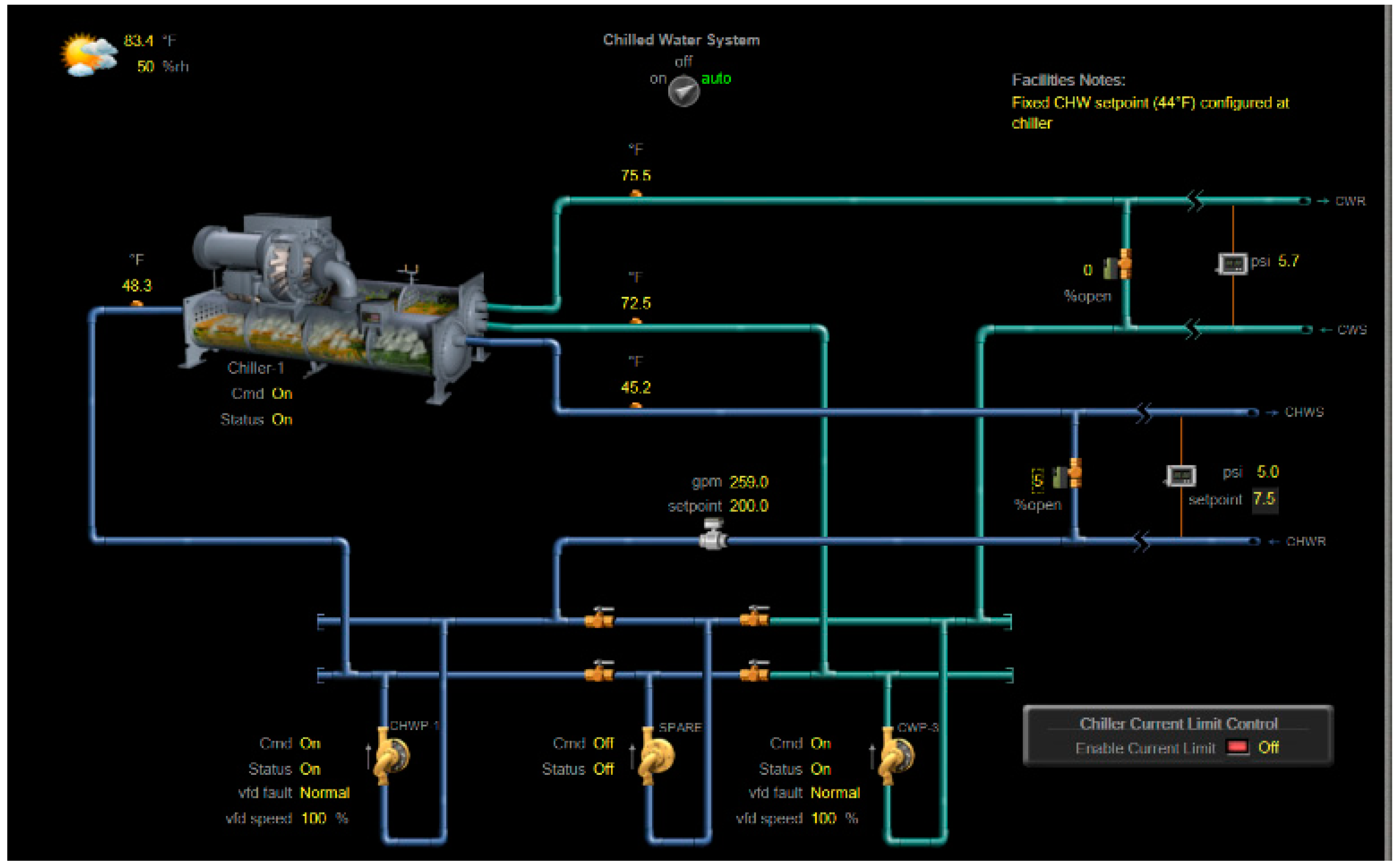
Chiller plant system: The variable primary flow (VPF) system is used in the chiller plant in Nesbitt Hall. In the chiller plant, one chiller, one primary pump (variable speed), one spare pump (constant speed) provide chilled water for AHU_1, AHU_2, and AHU_3 in the building. Figure A2 shows the configuration of the chiller plant loop in Nesbitt Hall from the web interface of BAS. A cooling tower is installed on the roof to dispose of heat from the chiller.
Figure A2.
Configuration of the chiller plant loop in Nesbitt Hall from the web interface of a building automation system (BAS).
Figure A2.
Configuration of the chiller plant loop in Nesbitt Hall from the web interface of a building automation system (BAS).

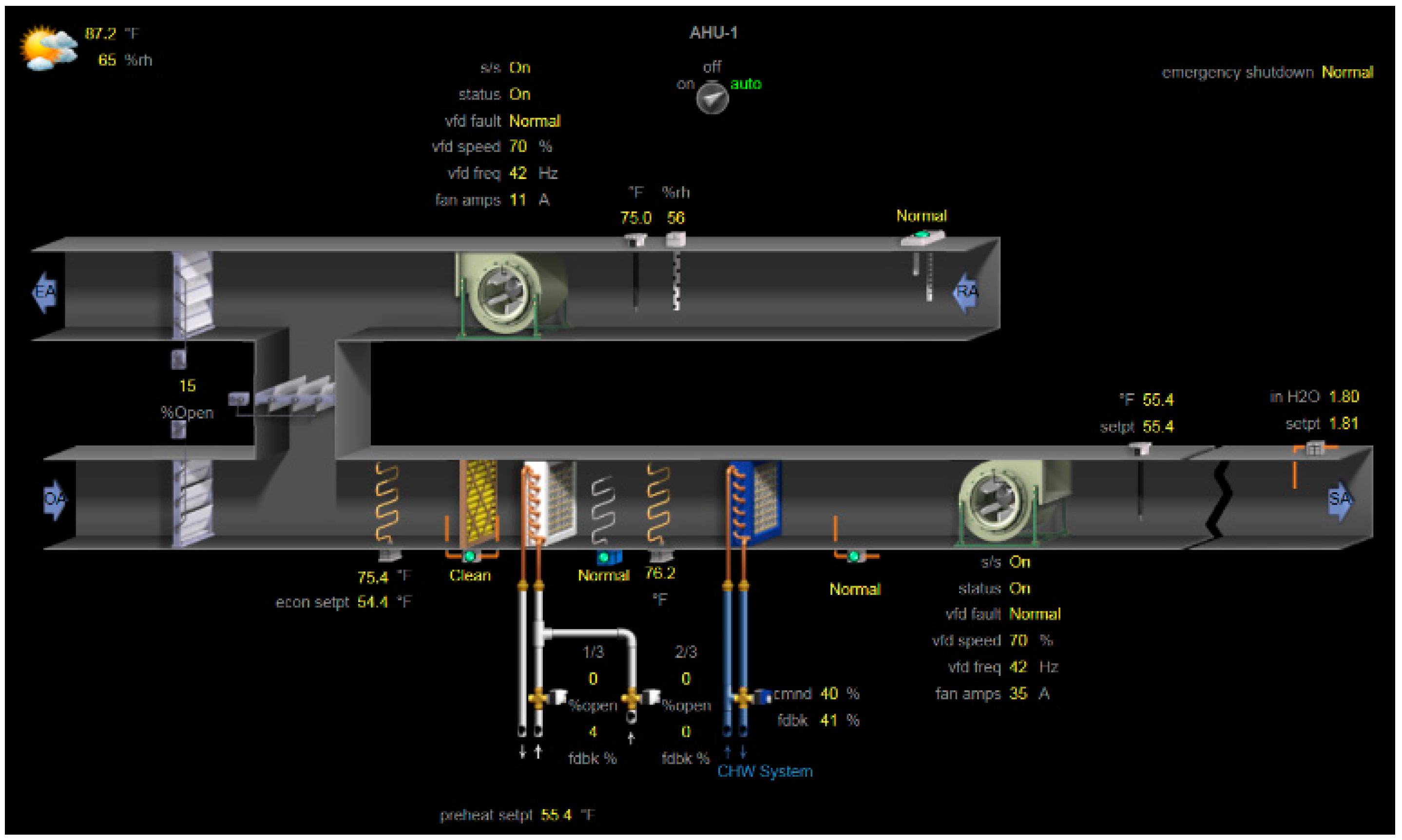
AHU system: The AHU regulates and circulates zone air to provide heating, cooling and ventilating in Nesbitt Hall. There are three AHUs in the Nesbitt Hall. AHU_1 and AHU_2 are equipped with returned air ducts. AHU_3 does not have a return air duct. AHU_1 is in the basement. AHU_2 and 3 are on the penthouse. Figure A3 provides the configuration of AHU_1 from the web interface of BAS.
Figure A3.
Configuration of AHU_1 in Nesbitt Hall from the web interface of BAS.

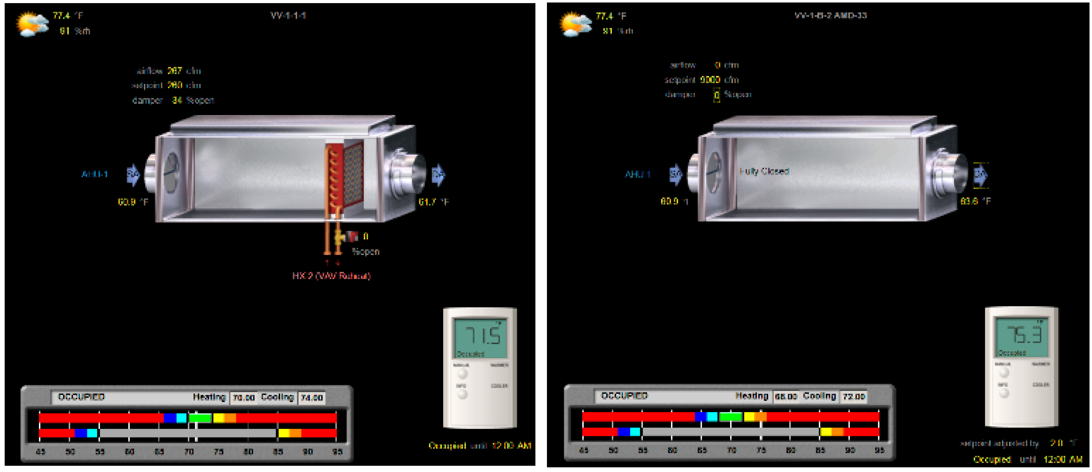
Air terminal system: Nesbitt Hall uses VAV system. As shown in Figure A4, two types of VAV boxes, with and without heating coils, are used in different zones to meet the requirement of the thermal load.
Figure A4.
The configuration of VAV box with and without reheat in Nesbitt Hall from the web interface of BAS.
Figure A4.
The configuration of VAV box with and without reheat in Nesbitt Hall from the web interface of BAS.

References
- EIA. Monthly Energy Review—June 2020; US Energy Information Administration: Washington, DC, USA, 2020. Available online: https://www.eia.gov/totalenergy/data/monthly/ (accessed on 1 July 2020).
- Zhang, L.; Wen, J. A systematic feature selection procedure for short-term data-driven building energy forecasting model development. Energy Build. 2019, 183, 428–442. [Google Scholar] [CrossRef]
- Gruenwald, L.; Chok, H.; Aboukhamis, M. Using data mining to estimate missing sensor data. In Proceedings of the Seventh IEEE International Conference on Data Mining Workshops (ICDMW 2007), Omaha, NE, USA, 28–31 October 2007. [Google Scholar]
- Cabrera, D.F.M.; Zareipour, H. Data association mining for identifying lighting energy waste patterns in educational institutes. Energy Build. 2013, 62, 210–216. [Google Scholar] [CrossRef]
- Efron, B. Missing data, imputation, and the bootstrap. J. Am. Stat. Assoc. 1994, 89, 463–475. [Google Scholar] [CrossRef]
- Pigott, T.D. A review of methods for missing data. Educ. Res. Eval. 2001, 7, 353–383. [Google Scholar] [CrossRef] [Green Version]
- Harel, O.; Zhou, X.H. Multiple imputation: Review of theory, implementation and software. Stat. Med. 2007, 26, 3057–3077. [Google Scholar] [CrossRef] [PubMed] [Green Version]
- Ibrahim, J.G.; Chen, M.-H.; Lipsitz, S.R.; Herring, A.H. Missing-data methods for generalized linear models: A comparative review. J. Am. Stat. Assoc. 2005, 100, 332–346. [Google Scholar] [CrossRef]
- Ekwevugbe, T.; Brown, N.; Pakka, V. Realt-time building occupancy sensing for supporting demand driven hvac operations. In Proceedings of the International Conference for Enhanced Building Operations (ICEBO), Montréal, QC, Canada, 8–11 October 2013. [Google Scholar]
- Xiao, F.; Fan, C. Data mining in building automation system for improving building operational performance. Energy Build. 2014, 75, 109–118. [Google Scholar] [CrossRef]
- Rahman, A.; Srikumar, V.; Smith, A.D. Predicting electricity consumption for commercial and residential buildings using deep recurrent neural networks. Appl. Energy 2018, 212, 372–385. [Google Scholar] [CrossRef]
- Peppanen, J.; Zhang, X.; Grijalva, S.; Reno, M.J. Handling bad or missing smart meter data through advanced data imputation. In Proceedings of the 2016 IEEE Power & Energy Society Innovative Smart Grid Technologies Conference (ISGT), Minneapolis, MN, USA, 6–9 September 2016. [Google Scholar]
- Ma, J.; Cheng, J.C.P.; Jiang, F.; Chen, W.; Wang, M.; Zhai, C. A bi-directional missing data imputation scheme based on LSTM and transfer learning for building energy data. Energy Build. 2020, 216, 109941. [Google Scholar] [CrossRef]
- Inman, D.; Elmore, R.; Bush, B. A case study to examine the imputation of missing data to improve clustering analysis of building electrical demand. Build. Serv. Eng. Res. Technol. 2015, 36, 628–637. [Google Scholar] [CrossRef]
- Schachinger, D.; Gaida, S.; Kastner, W.; Petrushevski, F.; Reinthaler, C.; Sipetic, M.; Zucker, G. An advanced data analytics framework for energy efficiency in buildings. In Proceedings of the 2016 IEEE 21st International Conference on Emerging Technologies and Factory Automation (ETFA), Berlin, Germany, 6–9 September 2016. [Google Scholar]
- Habib, U.; Zucker, G.; Blochle, M.; Judex, F.; Haase, J. Outliers detection method using clustering in buildings data. In Proceedings of the IECON 2015-41st Annual Conference of the IEEE Industrial Electronics Society, Yokohama, Japan, 9–12 November 2015. [Google Scholar]
- Xia, J.; Hong, T.; Shen, Q.; Feng, W.; Yang, L.; Im, P.; Lu, A.; Bhandari, M. Comparison of building energy use data between the United States and China. Energy Build. 2014, 78, 165–175. [Google Scholar] [CrossRef] [Green Version]
- Garnier, A.; Eynard, J.; Caussanel, M.; Grieu, S. Missing data estimation for energy resources management in tertiary buildings. In Proceedings of the CCCA12, Marseilles, France, 6–8 December 2012. [Google Scholar]
- Bradley, J.V. Distribution-Free Statistical Tests, 1st ed.; Prentice-Hall: Ann Arbor, MI, USA, 1968. [Google Scholar]
Figure 1.
Diagram of the developed data imputation framework with two modules.
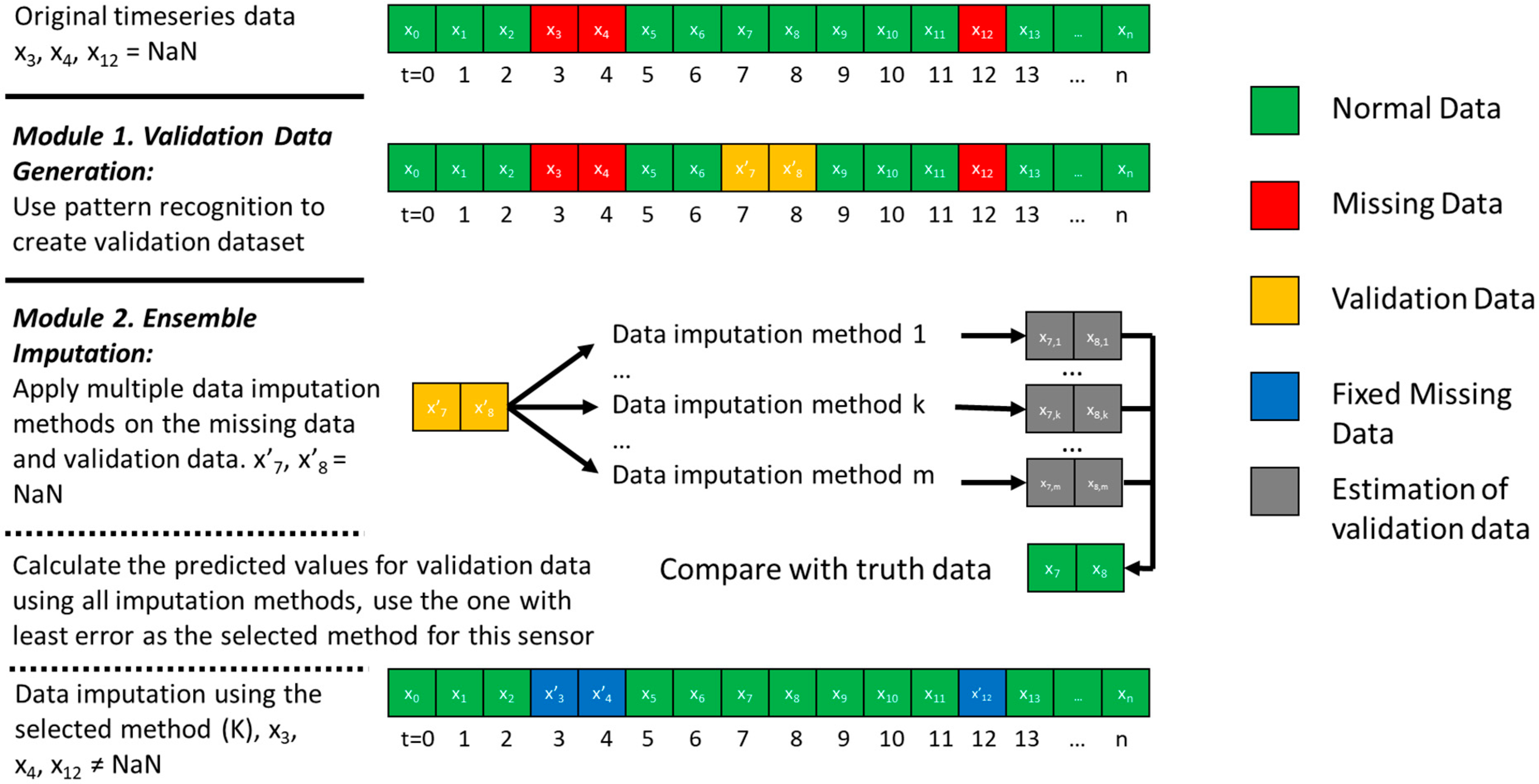
Figure 2.
Appearance of Nesbitt Hall.

Figure 3.
Example of missing data for whole building energy meter.

Figure 4.
Example of one real missing data point and one generated validation data point in the sensor chiller energy meter.
Figure 4.
Example of one real missing data point and one generated validation data point in the sensor chiller energy meter.
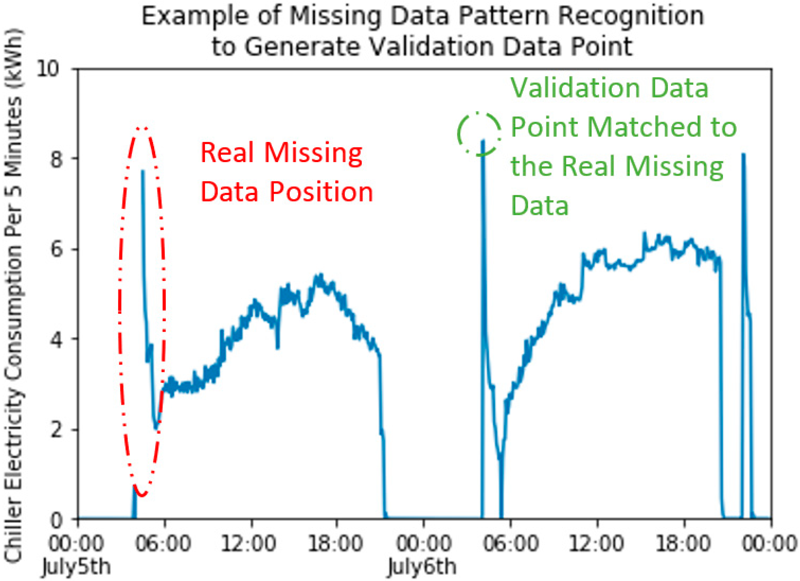
Table 1.
Sensors used in the case study of the developed framework.
| No. | Equipment | Sensor Type | Original Sensor Name from BAS | Sensor Description |
|---|---|---|---|---|
| 1 | Chiller | Energy meter | peco_meter/elec_usage_chiller | Chiller electricity consumption |
| 2 | Flow meter | chws_control/chw_flow | Chilled water flow rate | |
| 3 | Thermometer | chws_control/chws_temp | Chilled water supply temperature | |
| 4 | Differential pressure sensors | chws_control/delta_press | Chilled water supply and return pressure difference | |
| 5 | Cooling tower | Differential pressure sensors | chws_control/cw_delta_press | Cooling water supply and return pressure difference |
| 6 | Thermometer | chws_control/cwr_temp | Cooling water return temperature | |
| 7 | Valve position | chws_control/cw_vlv_fdbk | Cooling water valve feedback | |
| 8 | Fan status | ct_control/ct_fan_status/trend_log | Cooling tower fan status | |
| 9 | AHU | Thermometer | ahu1/ra_temp/trend_log | AHU 1 return air temperature |
| 10 | Valve position | ahu1/econ | AHU 1 economizer valve position | |
| 11 | Valve position | ahu1/chw_valve | AHU1 cooling coil valve position | |
| 12 | Humidity sensor | ahu1/ra_humidity | AHU1 return air humidity | |
| 13 | Ampere meter | ahu1/sfan_amps | AHU 1 supply air fan ampere | |
| 14 | Valve position | ahu1/htg_stm_vlv_1_3 | AHU 1 steam valve position | |
| 15 | Differential pressure sensors | ahu1/stat_press | AHU 1 supply air static pressure | |
| 16 | Thermometer | ahu1/pht_temp | AHU 1 preheat coil water temperature | |
| 17 | VAV | Flow meter | vv-1-b-1/air_flow/flow_input | VAV 1 air flow rate |
| 18 | Thermometer | vv-1-b-1/da_temp/trend_log | VAV 1 discharge air temperature |
Table 2.
Missing data description of the selected sensors.
| No | Sensor Name | Number of Missing Data | Maximum Hole Size |
|---|---|---|---|
| 1 | peco_meter/elec_usage_chiller | 466 | 2 |
| 2 | chws_control/chw_flow | 512 | 2 |
| 3 | chws_control/chws_temp | 439 | 1 |
| 4 | chws_control/delta_press | 505 | 2 |
| 5 | chws_control/cw_delta_press | 236 | 2 |
| 6 | chws_control/cwr_temp | 446 | 1 |
| 7 | chws_control/cw_vlv_fdbk | 531 | 3 |
| 8 | ct_control/ct_fan_status/trend_log | 426 | 1 |
| 9 | ahu1/ra_temp/trend_log | 466 | 1 |
| 10 | ahu1/econ | 269 | 2 |
| 11 | ahu1/chw_valve | 315 | 3 |
| 12 | ahu1/ra_humidity | 446 | 2 |
| 13 | ahu1/sfan_amps | 334 | 2 |
| 14 | ahu1/htg_stm_vlv_1_3 | 118 | 2 |
| 15 | ahu1/stat_press | 118 | 1 |
| 16 | ahu1/pht_temp | 236 | 2 |
| 17 | vv-1-b-1/air_flow/flow_input | 216 | 3 |
| 18 | vv-1-b-1/da_temp/trend_log | 571 | 1 |
Table 3.
Randomness of missing data (Z-score) for each sensor in terms of hour of day, month, and weekday indicator.
Table 3.
Randomness of missing data (Z-score) for each sensor in terms of hour of day, month, and weekday indicator.
| Sensor Name | Hour | Day | Weekday Indicator | Month | Average |
|---|---|---|---|---|---|
| peco_meter/elec_usage_chiller | 2.30 | 1.17 | 2.06 | 2.18 | 1.93 |
| chws_control/chw_flow | 2.26 | 0.79 | 2.01 | 2.15 | 1.80 |
| chws_control/chws_temp | 2.09 | 0.22 | 1.86 | 1.96 | 1.53 |
| chws_control/delta_press | 2.24 | 0.71 | 1.99 | 2.12 | 1.77 |
| chws_control/cw_delta_press | 1.53 | 0.57 | 1.26 | 1.35 | 1.18 |
| chws_control/cwr_temp | 2.11 | 0.27 | 1.80 | 1.97 | 1.54 |
| chws_control/cw_vlv_fdbk | 2.15 | 0.68 | 1.88 | 2.02 | 1.69 |
| ct_control/ct_fan_status/trend_log | 2.06 | 0.18 | 1.78 | 1.92 | 1.49 |
| ahu1/ra_temp/trend_log | 2.15 | 0.25 | 1.82 | 2.02 | 1.56 |
| ahu1/econ | 1.63 | 0.60 | 1.35 | 1.46 | 1.26 |
| ahu1/chw_valve | 1.77 | 0.82 | 1.41 | 1.61 | 1.40 |
| ahu1/ra_humidity | 2.11 | 0.68 | 1.83 | 1.99 | 1.65 |
| ahu1/sfan_amps | 1.82 | 0.55 | 1.43 | 1.67 | 1.37 |
| ahu1/htg_stm_vlv_1_3 | 1.08 | 0.36 | 0.61 | 0.86 | 0.73 |
| ahu1/stat_press | 1.08 | 0.01 | 0.59 | 0.82 | 0.62 |
| ahu1/pht_temp | 1.53 | 0.56 | 1.17 | 1.35 | 1.15 |
| vv-1-b-1/air_flow/flow_input | 1.46 | 0.70 | 1.18 | 1.27 | 1.15 |
| vv-1-b-1/da_temp/trend_log | 2.39 | 0.39 | 2.14 | 2.27 | 1.79 |
| Average | 1.85 | 0.49 | 1.54 | 1.70 | 1.39 |
Table 4.
Pool of data imputation methods for the case study.
| No. | Category | Abbreviation | Definition and Description | Library or Reference |
|---|---|---|---|---|
| 1 | Simple | bfill | use next valid observation to fill gap | pandas.DataFrame.fillna |
| 2 | Simple | ffill | use last valid observation to fill gap | pandas.DataFrame.fillna |
| 3 | Simple | nearest | Use the nearest available value | scipy.interpolate.interp1d |
| 4 | Linear | linear | Linear interpolation | pandas.DataFrame.interpolate |
| 5 | Nonlinear | quadratic | Interpolation of second order | scipy.interpolate.interp1d |
| 6 | Nonlinear | cubic | Interpolation of third order | scipy.interpolate.interp1d |
| 7 | Spline | piecewise_polynomial | Piecewise polynomial curve specified by points and derivatives | scipy.interpolate.PiecewisePolynomial |
| 8 | Spline | from_derivatives | Piecewise polynomial in the Bernstein basis | scipy.interpolate.BPoly.from_derivatives |
| 9 | Spline | pchip | Piecewise Cubic Hermite Interpolating Polynomial | scipy.interpolate.PchipInterpolator |
| 10 | Spline | akima | Akima spline interpolation | scipy.interpolate.Akima1DInterpolator |
| 11 | Machine learning | ANN | Use Multi-layer Perceptron to predict the missing value based on weather and time | sklearn.neural_network.MLPRegressor |
Table 5.
Summary of the performance (coefficient of variation of root mean squared error (CVRMSE)) of imputation methods for each sensor.
Table 5.
Summary of the performance (coefficient of variation of root mean squared error (CVRMSE)) of imputation methods for each sensor.
| Sensors\Imputation Methods | bfill | ffill | ANN | Linear | Nearest | Quadratic | Cubic | pp * | Fd * | pchip | akima | Avg * | Ensemble |
|---|---|---|---|---|---|---|---|---|---|---|---|---|---|
| peco_meter/elec_usage_chiller | 0.03 | 0.04 | 0.02 | 0.02 | 0.03 | 0.04 | 0.04 | 0.02 | 0.02 | 0.02 | 0.02 | 0.03 | 0.02 |
| chws_control/chw_flow | 0.43 | 0.33 | 0.14 | 0.23 | 0.27 | 0.26 | 0.27 | 0.23 | 0.23 | 0.23 | 0.24 | 0.26 | 0.14 |
| chws_control/chws_temp | 0.03 | 0.03 | 0.01 | 0.02 | 0.03 | 0.02 | 0.02 | 0.02 | 0.02 | 0.02 | 0.02 | 0.02 | 0.01 |
| chws_control/delta_press | 0.83 | 0.50 | 0.30 | 0.37 | 0.48 | 0.26 | 0.27 | 0.37 | 0.37 | 0.29 | 0.30 | 0.39 | 0.26 |
| chws_control/cw_delta_press | 0.07 | 0.14 | 0.02 | 0.05 | 0.04 | 0.04 | 0.05 | 0.05 | 0.05 | 0.04 | 0.04 | 0.05 | 0.02 |
| chws_control/cwr_temp | 0.01 | 0.01 | 0.01 | 0.01 | 0.01 | 0.02 | 0.02 | 0.01 | 0.01 | 0.01 | 0.01 | 0.01 | 0.01 |
| chws_control/cw_vlv_fdbk | 0.49 | 0.49 | 0.16 | 0.44 | 0.49 | 0.66 | 0.68 | 0.44 | 0.44 | 0.45 | 0.47 | 0.47 | 0.16 |
| ct_control/ct_fan_status/trend_log | 1.94 | 1.82 | 0.53 | 1.58 | 1.87 | 2.03 | 2.08 | 1.58 | 1.58 | 1.62 | 1.65 | 1.66 | 0.53 |
| ahu1/ra_temp/trend_log | 0.01 | 0.01 | 0.01 | 0.00 | 0.01 | 0.00 | 0.00 | 0.00 | 0.00 | 0.00 | 0.00 | 0.01 | 0.00 |
| ahu1/econ | 0.47 | 0.09 | 0.16 | 0.16 | 0.07 | 0.16 | 0.18 | 0.16 | 0.16 | 0.13 | 0.13 | 0.17 | 0.07 |
| ahu1/chw_valve | 0.26 | 0.28 | 0.11 | 0.12 | 0.06 | 0.19 | 0.20 | 0.12 | 0.12 | 0.09 | 0.09 | 0.15 | 0.06 |
| ahu1/ra_humidity | 0.04 | 0.04 | 0.02 | 0.02 | 0.03 | 0.02 | 0.02 | 0.02 | 0.02 | 0.02 | 0.02 | 0.03 | 0.02 |
| ahu1/sfan_amps | 0.13 | 0.16 | 0.09 | 0.08 | 0.09 | 0.08 | 0.08 | 0.08 | 0.08 | 0.08 | 0.08 | 0.09 | 0.08 |
| ahu1/htg_stm_vlv_1_3 | 0.16 | 0.10 | 0.06 | 0.10 | 0.08 | 0.10 | 0.12 | 0.10 | 0.10 | 0.09 | 0.10 | 0.10 | 0.06 |
| ahu1/stat_press | 0.06 | 0.13 | 0.09 | 0.06 | 0.13 | 0.16 | 0.17 | 0.06 | 0.06 | 0.07 | 0.07 | 0.10 | 0.06 |
| ahu1/pht_temp | 0.03 | 0.01 | 0.02 | 0.01 | 0.00 | 0.01 | 0.02 | 0.01 | 0.01 | 0.01 | 0.01 | 0.01 | 0.00 |
| vv-1-b-1/air_flow/flow_input | 0.44 | 0.52 | 0.26 | 0.23 | 0.43 | 0.23 | 0.25 | 0.23 | 0.23 | 0.21 | 0.25 | 0.30 | 0.21 |
| vv-1-b-1/da_temp/trend_log | 0.01 | 0.01 | 0.01 | 0.01 | 0.01 | 0.01 | 0.01 | 0.01 | 0.01 | 0.01 | 0.01 | 0.01 | 0.01 |
| Avg * | 0.30 | 0.26 | 0.11 | 0.19 | 0.23 | 0.24 | 0.25 | 0.19 | 0.19 | 0.19 | 0.19 | 0.21 | 0.09 |
* pp: piecewise_polynomial, fd: from_derivatives, avg: average.
Publisher’s Note: MDPI stays neutral with regard to jurisdictional claims in published maps and institutional affiliations. |
© 2020 by the author. Licensee MDPI, Basel, Switzerland. This article is an open access article distributed under the terms and conditions of the Creative Commons Attribution (CC BY) license (http://creativecommons.org/licenses/by/4.0/).
Share and Cite
MDPI and ACS Style
Zhang, L. A Pattern-Recognition-Based Ensemble Data Imputation Framework for Sensors from Building Energy Systems. Sensors 2020, 20, 5947. https://doi.org/10.3390/s20205947
AMA Style
Zhang L. A Pattern-Recognition-Based Ensemble Data Imputation Framework for Sensors from Building Energy Systems. Sensors. 2020; 20(20):5947. https://doi.org/10.3390/s20205947
Chicago/Turabian StyleZhang, Liang. 2020. "A Pattern-Recognition-Based Ensemble Data Imputation Framework for Sensors from Building Energy Systems" Sensors 20, no. 20: 5947. https://doi.org/10.3390/s20205947
Note that from the first issue of 2016, this journal uses article numbers instead of page numbers. See further details here.